Multiscale Adjacent Superpixel-Based Extended Multi-Attribute Profiles Embedded Multiple Kernel Learning Method for Hyperspectral Classification

Abstract

In this paper, superpixel features and extended multi-attribute profiles (EMAPs) are embedded in a multiple kernel learning framework to simultaneously exploit the local and multiscale information in both spatial and spectral dimensions for hyperspectral image (HSI) classification. First, the original HSI is reduced to three principal components in the spectral domain using principal component analysis (PCA). Then, a fast and efficient segmentation algorithm named simple linear iterative clustering is utilized to segment the principal components into a certain number of superpixels. By setting different numbers of superpixels, a set of multiscale homogenous regional features is extracted. Based on those extracted superpixels and their first-order adjacent superpixels, EMAPs with multimodal features are extracted and embedded into the multiple kernel framework to generate different spatial and spectral kernels. Finally, a PCA-based kernel learning algorithm is used to learn an optimal kernel that contains multiscale and multimodal information. The experimental results on two well-known datasets validate the effectiveness and efficiency of the proposed method compared with several state-of-the-art HSI classifiers.

1. Introduction

At present, hyperspectral images (HSIs) are attracting increasing attention. With the fast iteration of hyperspectral sensors, researchers can easily collect a large amount of HSI data having high spatial resolution and multiple bands that form high-dimensional features, such as complex and fine geometrical structures [1,2]. These characteristics encourage the wide use of HSIs for various thematic applications, such as military object detection, precision agriculture [3], biomedical technology, and geological and terrain exploration [4,5]. As one of the basic methods for the above applications, HSI classification plays an important role and has made certain developments in the past few decades [6].

Many classic machine learning methods can be directly applied to the classification of HSIs, such as naive Bayes, decision trees, K-nearest neighbor (KNN), wavelet analysis, support vector machines (SVMs), random forest (RF), regression trees, ensemble advancement, and linear regression [7,8,9]. However, these methods either treat the HSI as a combination of several hundreds of gray images and extract the corresponding features for classification or use only spectral features for classification, thus producing unsatisfactory results [6].

Recently, classification methods for HSIs based on sparse representation have attracted the attention of researchers [10]. Many well-performing sparse representation classification (SRC) methods have been developed. SRC assumes that each spectrum can be sparsely represented by spectra belonging to the same class and then obtains a good approximation of the original data through a corresponding algorithm [11,12]. Therefore, more and more scholars have used the sparse representation technique to conduct HSI classification. Due to the irrationality of the traditional joint KNN algorithm for setting the same weights in the same region, Tu et al. proposed a weighted joint nearest neighbor sparse representation algorithm [13]. Later, a self-paced joint sparse representation (SPJSR) model was proposed. The least-squares loss used in the classical joint sparse representation model was changed to a weighted least-squares loss, and a self-paced learning strategy was employed to automatically determine the weights of the adjacent pixels [14]. Because different scales of a region in an HSI contain complementary and correlated knowledge, Fang et al. proposed an adaptive sparse representation method using a multiscale strategy [15]. To make full utilization of the spatial correlation of HSI and improve the classification accuracy, in [16], Dundar et al. proposed a multiscale superpixel and guided filter-based spatial-spectral HSI classification method. However, when the sample size is small, SRC will ignore the cooperative representation of other categories of samples, resulting in an incomplete dictionary for each category of samples, which produces a larger residual in the results. To alleviate this problem, the cooperative representation method (CRC) was presented by researchers. Compared to SRC, the $L_2$ norm used by the CRC not only has discriminability like that of SRC, but also has lower computational complexity. Using the collaborative representation, Jia et al. proposed a multiscale superpixel-based classification method [17]. To further improve the accuracy of HSI classification, Yang et al. proposed a joint collaborative representation method using a multiscale strategy and a locally adaptive dictionary [18]. Considering the correlation between different classes of HSIs, with the assistance of Tikhonov regularization, a discriminative kernel collaborative representation method was proposed by Ma et al. [19] that utilized nuclear collaborative representation for HSI classification. More recently, low rank representation (LRR) has been studied by scholars in the field of HSI classification. To fully exploit the local geometric structure in the data, Wang et al. proposed a novel LRR model with regularized locality and structure [20]. Meanwhile, a new self-supervised low-rank representation algorithm was proposed by Wang et al. for further improvement of HSI classification [21]. Moreover, Ding et al. proposed a sparse low-rank representation method that relied on key connectivity for HSI classification [22]. This study combined low-rank representation and sparse representation while retaining the connectivity of key representations within classes. To decrease the impact of spectral variation on subsequent spectral analyses, Mei et al. conducted anti-coagulation research within coherent spatial and spectral low-rank representation, which effectively suppressed the class spectral variations [23].

As one of the hottest feature extraction techniques, deep learning has made excellent progress in computer vision and image processing applications [24,25,26,27]. Currently, deep learning is also becoming more popular in the field of HSI classification [28]. HSI data consist of multi-dimensional spectral cubes that contain much useful information, so the intrinsic features of the image are easily extracted by deep learning techniques [29]. For instance, the currently popular convolutional neural network (CNN) model has produced excellent HSI classification results [30,31]. In addition, some improved HSI classification methods have been proposed based on deep learning. For instance, by combining active learning and deep neural networks, Liu et al. proposed an effective framework for HSI classification, where the deep belief network (DBN) was employed to extract the deep features hidden in the spectral dimension [32]. Then, a learning classifier was used to refine those training samples to boost their quality. Zhong et al. further enhanced the DBN model and proposed a diversified DBN model [33]. In their design, the pre-training and tuning procedures of the DBN were regularized to achieve better classification accuracy. Moreover, 1D CNN [34,35] and 1D generative antagonistic networks [36,37] were also employed to describe the spectral features of the HSI. However, deep learning methods also have some problems; for example, they usually need many training samples, and the extracted features are not always interpretable. Therefore, the trend of subsequent research is to combine traditional feature extraction methods with deep learning methods to obtain more accurate classification results.

Another, more powerful classification technique for the HSI is the kernel method, especially the composite kernel (CK) method. In the actual classification process, samples in the original space are often not linearly separable [38]. Therefore, to solve the problem of linear inseparability, the kernel method is used to map the samples to a higher dimensional feature space so that the samples are linearly separable [39]. Certainly, the performance of the kernel method depends largely on the kernel selection. For example, the Gaussian kernel and the polynomial kernel are common kernels, and they are often not flexible enough to reflect the comprehensive features of the data [40]. Moreover, with increasing requirements of classification accuracy, a single kernel with a specific function cannot deliver a satisfactory result [41]. To solve this problem, the CK was proposed. It combines two or more different features, such as the global and local kernel, or the local kernel and spectral kernel, into a kernel composition framework for HSI classification [42]. Sun et al. proposed a CK classification method using spatial-spectral information and abundance information in the HSI [43]. For intrinsic image decomposition of the HSI, Jin et al. put forward a new optimization algorithm, and the CK learning method was then utilized to combine reflectance with the shading component [44]. Furthermore, Chen et al. proposed a spatial-spectral composite feature broad learning system classification method [45]. This method inherits the advantages of a broad learning system and is well-suited to multi-class tasks. As the most widely-used classier, SVM can also bring excellent classification accuracy to the HSI [46]. Huang et al. proposed an SVM-based method for HSI classification [47]. In this work, weighted mean reconstruction and CKs were combined to explore the spatial-spectral information in the HSI. With the continuous development of superpixel segmentation technology, Duan et al. further improved edge-preserving features by considering the inter- and intra-spectral properties of superpixels and formed one CK for the spectral and edge-preserving features [48]. Because the HSI contains many spectral bands, mapping the high-dimensional data to achieve improved classification speed has been of great concern in recent years. To address this problem, Tajiri et al. proposed a fast patch-free global learning kernel method based on a CK method [49]. Compared with the original single-kernel method, the CK function has the following obvious advantages: (1) it maps the data into a complex nonlinear space to extract more useful information and make the data separable; (2) it provides the flexibility to include multiple and multimodal features.

Different from a CK in which only one kernel function is constructed to contain both spatial and spectral information, the spatial-spectral kernel (SSK) constructs two clusters in kernel space, thus capturing the hidden manifold in the HSI [50]. For example, the spatial-spectral weighted kernel embedded manifold distribution alignment method constructs a complex kernel with different weights for the spatial kernel and the spectral kernel [51]. The spatial-spectral multiple-kernel learning method utilizes extended morphological profiles (EMPs) as spatial features and the original spectra as spectral features. In this way, multiscale spatial and spectral kernel methods are formed [52]. In addition, the joint classification methods for HSIs based on spatial-spectral kernels and multi-feature fusion are especially suitable for a limited number of training samples [53]. Generally, the CK method and the SSK method adopt square windows or superpixel technology to extract spatial information. However, both methods may misclassify the pixels at the class boundary. To alleviate this problem, several methods for selecting adaptive neighborhood pixels to construct the spatial-spectral kernel have been proposed, which further improved classification performance [54,55]. For those CK or SSK methods, determining the weights of the base kernels is another difficult and urgent challenge. Therefore, many scholars have proposed multiple kernel learning methods, where the core idea is to obtain a linear optimal combination of those base kernels using an optimization algorithm [56,57,58].

In this study, following the line of the multiple kernel learning framework, we propose a novel multiscale, adjacent superpixel-based embedded multiple kernel learning method with the extended multi-attribute profile (MASEMAP-MKL) for HSI classification. The proposed method makes full use of superpixels and the EMAP to exploit multiscale and multimodal spatial and spectral features for the generation of multiple kernels. For the spatial information, both the superpixel and its first-order neighborhood superpixels are utilized to extract geometric features at different scales and combine the EMAP features to construct different base kernels. Finally, a principal component analysis (PCA)-based multiple kernel learning method is employed to determine the optimal weights of the base kernels. The main contributions of the proposed MASEMAP-MKL method are summarized as follows.

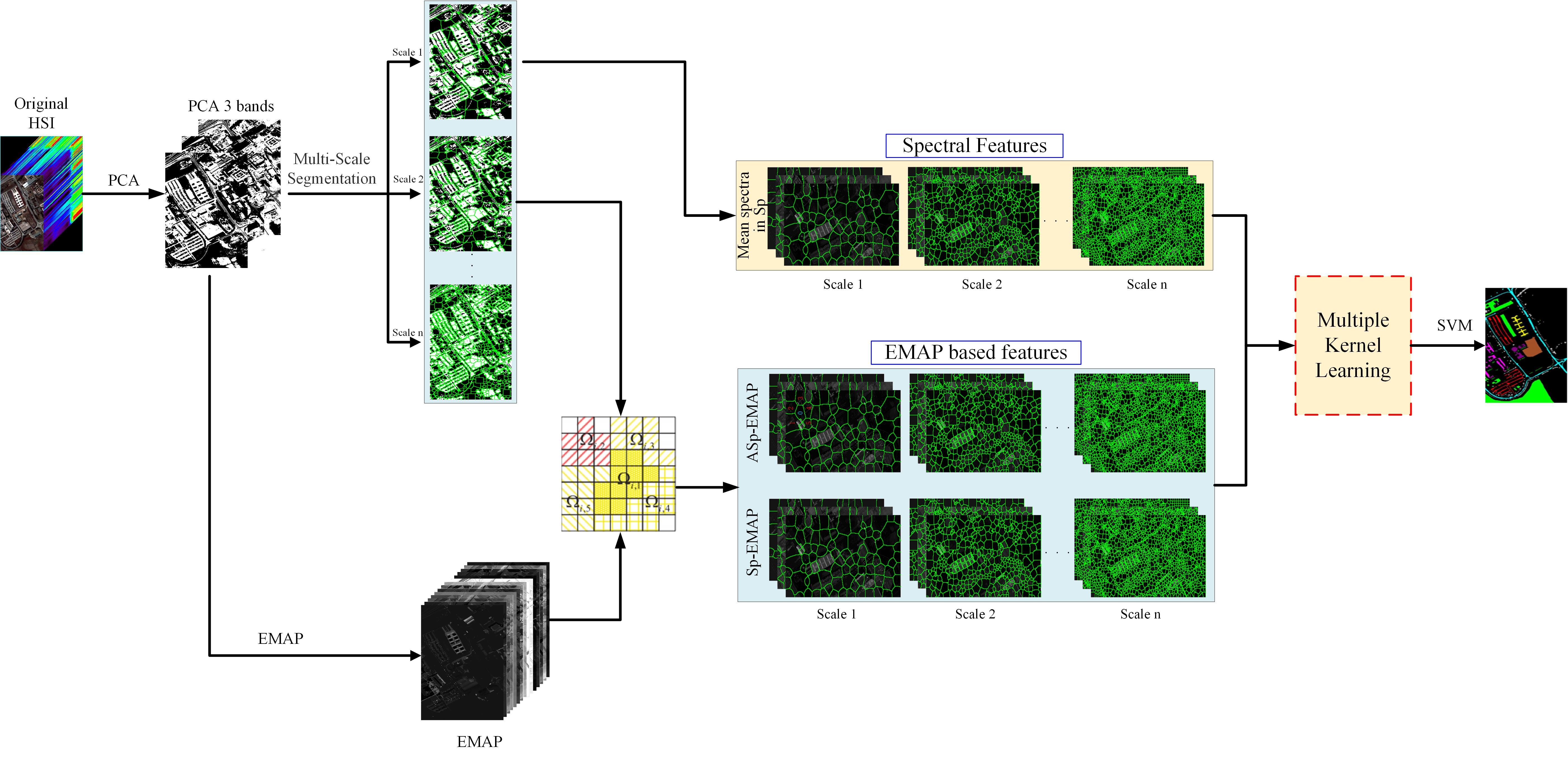
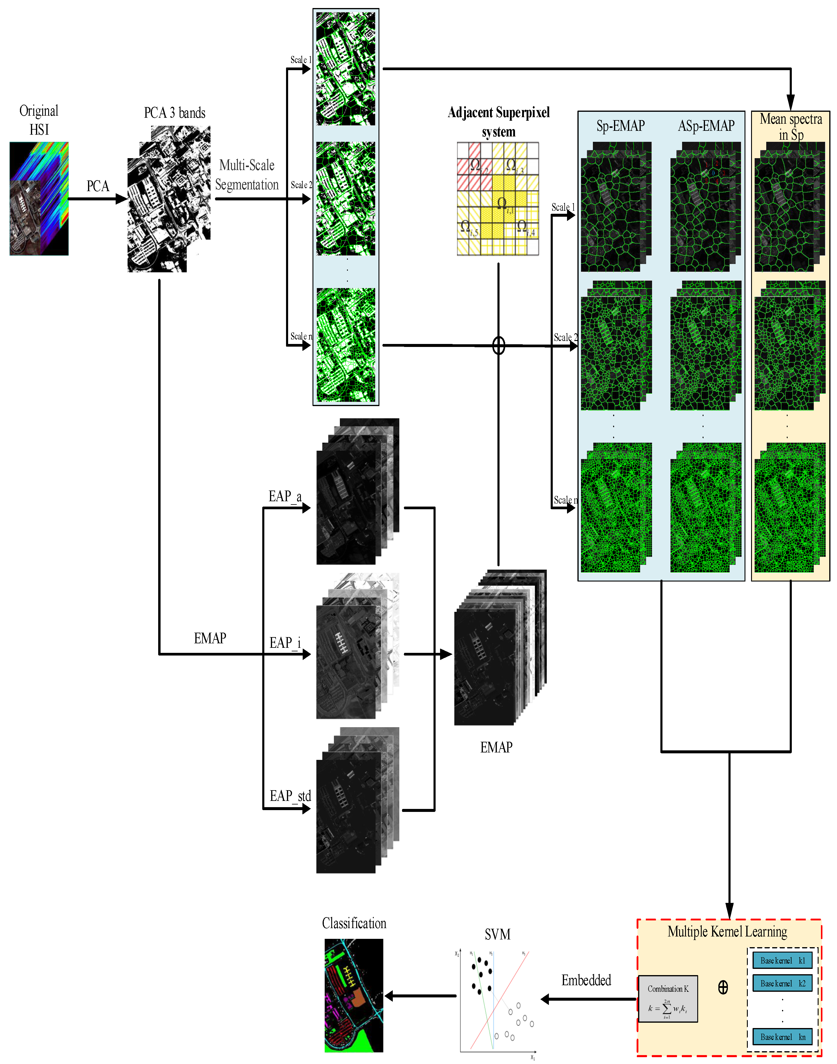
• The superpixel segmentation is used to extract geometric structure information in the HSI, and multiscale spatial information is simultaneously extracted according to the number of superpixels. In addition, the spectral feature of each pixel is replaced by the average of all the spectra in its superpixel, which is used to construct a superpixel-based mean spectral kernel.
• The EMAP features, together with the multiscale superpixels and the adjacent superpixels obtained above, are used to construct the superpixel morphological kernel and the adjacent superpixel morphological kernel. At this stage, multiscale features and multimodal features are fused together to construct three different kernels for classification.
• The multiple kernel learning technique is used to obtain the optimal kernel for HSI classification, which is a linear combination of all the above kernels.
• An experimental evaluation with two well-known datasets illustrates the computational efficiency and quantitative superiority of the proposed MASEMAP-MKL method in terms of all classification accuracies.

2. Materials and Methods

2.1. Preliminary Formulation

2.1.1. Kernelized Support Vector Machine

As a two class classification model, the basic principle of SVM is to classify data by solving the convex quadratic programming problem in the feature space. The kernelized SVM introduces a kernel function based on the SVM, which simplifies the calculation of the complicated vector inner product in the original space and directly calculates the inner product in the feature space. Specifically, given a set of labeled samples in HSIs, i.e., $\{({\mathbf{x}}_1,y_1),({\mathbf{x}}_2,y_2),\dots ,({\mathbf{x}}_N,y_N)\}$, where ${\mathbf{x}}_i\in {\mathbb{R}}^{L\times 1}$ is the i-th labeled spectrum and L is the number of bands, $y_i\in \{-1,1\}$ for $i\in \{1,2,\dots ,N\}$, and N is the number of all labeled samples in the scene. Therefore, the classification function of the kernelized SVM is formulated as:

$$f\left(\mathbf{x}\right)=\sum _{i=1}^N{\alpha }_i{y}_{i}K({\mathbf{x}}_i,\mathbf{x})+b$$

(1)

where $\alpha$ denotes the Lagrangian duality parameter, $K({\mathbf{x}}_i,\mathbf{x})$ denotes a kernel function, and b denotes the bias parameter. Then, we obtain the objective function as:

$$\begin{array}{c}\hfill \begin{array}{cc}\hfill \underset{\alpha }{argmax}& \sum _{i=1}^N{\alpha }_i-\frac{1}{2}\sum _{i,j=1}^N{\alpha }_i{\alpha }_j{y}_i{y}_{j}K({\mathbf{x}}_i,{\mathbf{x}}_j)\hfill \\ \hfill s.t.,& 0\le {\alpha }_i\le \beta ,i=1,\dots ,n\hfill \\ \hfill & \sum _{i=1}^N{\alpha }_i{y}_i=0\hfill \end{array}\end{array}$$

(2)

where $\beta$ is a parameter that controls the weight between two items in the objective function (e.g., to find the hyperplane with the largest margin and to guarantee the smallest deviation of the data points). Usually, the value of $\beta$ is determined manually and in advance. Under the above two constraint conditions, the most suitable values of $\alpha$ and l are obtained to get an optimal classifier. Our commonly used kernel functions are as follows.

The first one is the Gaussian kernel function:

$$K({\mathbf{x}}_i,{\mathbf{x}}_j)=exp\left\{-\frac{\left|\right|{\mathbf{x}}_i-{\mathbf{x}}_j{\left|\right|}_2^2}{2{\sigma }^2}\right\}$$

(3)

This kernel function maps the original space to an infinite-dimensional space. We can control the mapping dimension flexibly by adjusting the value of parameter $\sigma$.

The second kernel function is the polynomial kernel function:

$$K({\mathbf{x}}_i,{\mathbf{x}}_j)={(\alpha {\mathbf{x}}_i^T{\mathbf{x}}_j+C)}^d$$

(4)

where C denotes an offset parameter and d is an integer. We can change the dimension of the mapping by setting the value of d. When the value of d is one, the kernel function degrades to a linear kernel function. The linear kernel function is actually an SVM in the case of linear separability, which can only process linear data. In this situation, the classifier degrades to the most primitive SVM.

2.1.2. Superpixel Segmentation

A superpixel is a sub-region of the image that is local, consistent, and able to maintain certain local structural characteristics of the image. Superpixel segmentation is the process of aggregating pixels into a superpixel. Compared with a pixel, the basic unit of traditional processing methods, a superpixel is not only more conducive to the extraction of local features and the expression of structural information, but can also greatly reduce the computational complexity of subsequent processing. Achanta and others proposed simple linear iterative clustering (SLIC), which is based on the relationship between color similarity and spatial distance [59]. Firstly, J initial clustering centers are uniformly initialized in the image, and all pixels are labeled with the nearest cluster center. Therefore, the normalized distance based on color and spatial location features is:

$$d(i,j)=\sqrt{{\left(\frac{∥{\mathbf{c}}_i-{\mathbf{c}}_j∥}{n_c}\right)}^2+{\left(\frac{∥{\mathbf{s}}_i-{\mathbf{s}}_j∥}{n_s}\right)}^2}$$

(5)

In the formula, vector $\mathbf{c}$ represents the 3D color feature vector in the CIELAB color space. The vector $\mathbf{s}$ represents the two-dimensional spatial position coordinates. The subscript $j=1,2,\dots ,J$ is the label of the cluster center. The subscript i is the pixel label in the 2 s × 2 s neighborhood corresponding to the cluster center j, and $s=\sqrt{N/J}$, where N is the total number of image pixels. $n_c$ and $n_s$ are normalization constants for the color and space distance, respectively. After the initial clustering, the clustering center ${\phi }_j$ is updated iteratively according to the mean values of all the pixels’ color and spatial features in the corresponding clustering HSI block $G_j$.

$${\phi }_j=\frac{1}{n_j}\sum _{i\in G_j}\left[\begin{array}{c}{\mathbf{c}}_i\\ {\mathbf{s}}_i\end{array}\right]$$

(6)

where $n_j$ is the number of pixels in the image block $G_j$. This formula iteratively clusters and updates until the termination conditions are met. Finally, a neighbor merging strategy is used to eliminate the isolated small size superpixels, which ensures the compactness of the results.

2.1.3. EMAP

Based on mathematical morphology, Mauro et al. [60] proposed a method using the EMAP and independent component analysis. Compared with PCA, this method is more suitable for modeling the different information sources in the scene, and the classification accuracy obtained is higher. Later, Stijn et al. [61] proposed computing extended attribute profiles (EAPs) on features derived from supervised feature extraction methods. Song et al. [62] proposed a new image data classification strategy-decision fusion method that combines a complete classifier with extended multi-attribute morphological profiles to optimize the classification results.

The attribute profile (AP) is an extension of the morphological profile (MP), which is obtained by processing a scalar grayscale image f (such as each band image of an HSI or one principal component (PC) of an HSI), according to a criterion t with morphological attribute thickening (${\varphi }^t$) and n attribute thinning (${\gamma }^t$) operators:

$$AP\left(f\right)=\left\{{\varphi }_n^t\left(f\right),{\varphi }_{n-1}^t\left(f\right),\dots ,{\varphi }_1^t\left(f\right),f,{\gamma }_1^t\left(f\right),\dots ,{\gamma }_{n-1}^t\left(f\right),{\gamma }_n^t\left(f\right)\right\}$$

(7)

Analogous to the definition of the extended MPs (EMPs), EAPs are generated by concatenating many APs. Each AP is computed on one of the q PCs extracted by the PCA of an HSI:

$$EAP=\left\{AP\left(P{C}_1\right),AP\left(P{C}_2\right),\dots ,AP\left(P{C}_q\right)\right\}$$

(8)

An EMAP is composed of m different EAPs based on different attributes ($a_1,a_2,...,a_m$):

$$EMAP=\left\{EA{P}_{a_1},EA{P}_{a_2},\dots ,EA{P}_{a_m}\right\}$$

(9)

where $EA{P}_{a_i}=EA{P}_{a_i}/\left\{P{C}_1,P{C}_2,...,P{C}_q\right\}$ means calculating the $EAP$ on each PC of the HSI with attribute $a_i$. The value of q is usually set to be smaller than three. Three attributes, i.e., area, inertia, and the standard deviation, are used in the proposed method to extract different spatial information from the HSI.

2.1.4. CK

The CK usually takes the spectral mean or the variance of the neighborhood pixels as the spatial spectral characteristics and then forms the CK through the following core combination methods.

(1)

Stacked characteristic kernel: In this design, both the spectral and spatial features are directly stacked together as sample features.

$$K_{CK}^{s,w}=K({\mathbf{x}}_i,{\mathbf{x}}_j)=<\varphi \left({\mathbf{x}}_i\right),\varphi \left({\mathbf{x}}_j\right)>$$

(10)

(2)

Direct addition kernel: The spatial feature after nonlinear mapping is juxtaposed with the spectral feature as the feature of a high-dimensional space.

$$\begin{array}{cc}\hfill K_{CK}({\mathbf{x}}_i,{\mathbf{x}}_j)& =<\varphi \left({\mathbf{x}}_i\right),\varphi \left({\mathbf{x}}_j\right)>\hfill \\ & =<{\varphi }_1\left({\mathbf{x}}_i^{spe}\right),{\varphi }_2\left({\mathbf{x}}_i^{spa}\right),{\varphi }_1\left({\mathbf{x}}_j^{spe}\right),{\varphi }_2\left({\mathbf{x}}_j^{spa}\right)>\hfill \\ & =K^s({\mathbf{x}}_i^{spe},{\mathbf{x}}_j^{spe})+K^w({\mathbf{x}}_i^{spa},{\mathbf{x}}_j^{spa})\hfill \end{array}$$

(11)

(3)

Weighted summation kernel: By assigning different weights to the spatial and spectral features, $\mu$ is the weight parameter of the balanced spatial and spectral kernel. The weighted summation kernel can be constructed as follows:

$$K_{CK}({\mathbf{x}}_i,{\mathbf{x}}_j)=\mu K^s({\mathbf{x}}_i^{spe},{\mathbf{x}}_j^{spe})+(1-\mu )K^w({\mathbf{x}}_i^{spa},{\mathbf{x}}_j^{spa})$$

(12)

2.2. The Proposed MASEMAP-MKL Method

In this section, we propose a novel multiscale adjacent superpixel-based EMAP embedded multiple kernel learning method named MASEMAP-MKL for HSI classification. The flowchart of the proposed MASEMAP-MKL is shown in Figure 1. Two steps are performed as follows.

2.2.1. Adjacent Superpixel-Based EMAP Generation

The first step is the generation of the adjacent superpixel-based EMAP. Three different image features, i.e., the mean superpixel spectral feature, the superpixel morphological feature, and the adjacent superpixel morphological feature, are given.

(1)

Superpixel-based mean spectral feature:

After superpixel segmentation, the PC images are divided as $sp=\{s{p}_1,s{p}_2,\dots s{p}_J\}$, where J is the number of superpixels. We employ the local mean operator to obtain the superpixel-based mean spectral feature of a given spectrum in $s{p}_i$, which is formulated as:

$$\begin{array}{cc}\hfill {\mathbf{x}}_i^{sp-mean}& =\sum _{j=1}^{n_i}{\mathbf{x}}_j/\phantom{{\mathbf{x}}_i{n}_i}{n}_i,\hfill \\ \hfill {\mathbf{x}}_j& \in s{p}_i\hfill \end{array}$$

(13)

where $n_i$ is the number of pixels in the i-th superpixel. Therefore, after implementing the local mean operator for all superpixels, the obtained average features constitute the superpixel-based mean spectral feature of the HSI.

(2)

Superpixel-based morphological feature:

Enforcing the EMAP feature extraction operation on the segmented multiscale superpixel produces the superpixel morphological feature:

$${\mathbf{x}}_i^{sp-EMAP}=\sum _{i=1}^{n_i}{\mathbf{x}}_i^{EMAP}/\phantom{{\mathbf{x}}_i^{EMAP}{n}_i}{n}_i$$

(14)

where ${\mathbf{x}}_i^{EMAP}$ represents the EMAP feature vector. The superpixel morphological feature inherits the advantages of superpixel segmentation and morphological features at the same time and achieves a more thorough description of spatial information during classification.

(3)

Adjacent superpixel-based morphological feature:

Based on the superpixel morphological feature, we further empower the adjacent superpixel strategy to obtain adjacent superpixel morphological features; thus, the fusion of multiscale feature and multimodal features is realized for classification. The adjacent superpixel set is defined as:

$${\mathbf{x}}_i^{asp}=\{{\mathbf{x}}_i^{s{p}_1},{\mathbf{x}}_i^{s{p}_2},\dots {\mathbf{x}}_i^{s{p}_r}\}$$

(15)

where r is the number of adjacent superpixels with respect to the central superpixel ${\mathbf{x}}_i^{s{p}_i}$. Because the mean pixels are the representative feature of the superpixel, after calculating the mean pixels of the superpixels in ${\mathbf{x}}_i^{asp}$, the weighted adjacent superpixel morphological feature can be obtained by calculating the weighted mean pixel of the central adjacent superpixel:

$${\mathbf{x}}_i^{asp-EMAP}=\sum _{j=1}^r{\omega }_{i,j}\times {\mathbf{x}}_j^{sp-mean}$$

(16)

where ${\omega }_{i,j}$ is the weight of adjacent superpixel ${\mathbf{x}}_i^{s{p}_j}$ with respect to the central superpixel ${\mathbf{x}}_i^{s{p}_i}$, which is obtained by:

$${\omega }_{i,j}=\frac{exp\left(-\frac{SAD({\mathbf{x}}_j^{sp-mean}-{\mathbf{x}}_i^{sp-mean})}{h}\right)}{{\displaystyle \sum _{j=1}^r}exp\left(-\frac{SAD({\mathbf{x}}_j^{sp-mean}-{\mathbf{x}}_i^{sp-mean})}{h}\right)}$$

(17)

Unlike most studies that use the Euclidean distance to measure the distance between pixels, we use the spectral angle distance (SAD) to further explorer the spectral correlation of the HSI, which is denoted as:

$$SAD({\mathbf{x}}_j^{sp-mean}-{\mathbf{x}}_i^{sp-mean})=arccos\frac{({\mathbf{x}}_j^{sp-mean}{)}^T·{\mathbf{x}}_i^{sp-mean}}{∥{\mathbf{x}}_j^{sp-mean}∥·∥{\mathbf{x}}_i^{sp-mean}∥}$$

(18)

The above three different features achieve a more comprehensive description of the local and multiscale spatial-spectral information, and the richer features bring higher classification accuracy.

2.2.2. Multiscale Kernel Generation

For each pixel, we can obtain the three feature kernels according to the above Equations (13), (14), and (16), that is the superpixel-based mean spectral feature kernel $K^{sp-mean}$, the superpixel-based mean EMAP feature kernel $K^{sp-EMAP}$, and the adjacent superpixel-based weighted EMAP feature kernel $K^{ASP-EMAP}$. Then, by setting different number of superpixels, we can obtain the corresponding kernels at each scale. That is,

$$\{K_1^{sp-mean},\dots ,K_i^{sp-mean},\dots ,K_{m1}^{sp-mean}\}$$

(19)

$$\{K_1^{sp-EMAP},\dots ,K_i^{sp-EMAP},\dots ,K_{m2}^{sp-EMAP}\}$$

(20)

$$\{K_1^{asp-EMAP},\dots ,K_i^{asp-EMAP},\dots ,K_{m3}^{asp-EMAP}\}$$

(21)

Here, $m1,m2,m3$ are three parameters related to the scales for the superpixels of the corresponding features. For simplicity, we let $m=m1=m2=m3$ represent the multiscale for the superpixels of all three features.

So far, we have the kernels of different scales corresponding to the three features. To fuse all the above kernels, we use a linear combination to obtain an optimal kernel for HSI classification.

$$K^{MASPEMAP}=\sum _{i=1}^m{w}_i^1{K}_i^{sp-mean}+w_i^2{K}_i^{sp-EMAP}+w_i^3{K}_i^{asp-EMAP}$$

(22)

where $w_i^1$, $w_i^2$, and $w_i^3$ are the weights that control the ratio of the three kinds of kernels.

2.2.3. Multiple Kernel Learning Based on PCA

From Equation (22), we know that the optimal kernel is completely determined by the weights of the base kernels. Because $K^{MASPEMAP}$ is the linear combination of the base kernels, we can employ the multiple kernel learning method based on PCA to solve it, and we can directly use the first principal component of the PCA of the matrix composed of all base kernels as the optimal kernel, that is,

$$\begin{array}{cc}\hfill K^{MASEMAP}=PC{A}_1\left(\right[& K_1^{sp-mean},\dots ,K_i^{sp-mean},\dots ,K_{m1}^{sp-mean};\hfill \\ & K_1^{sp-EMAP},\dots ,K_i^{sp-EMAP},\dots ,K_{m2}^{sp-EMAP};\hfill \\ & K_1^{asp-EMAP},\dots ,K_i^{asp-EMAP},\dots ,K_{m3}^{asp-EMAP}\left]\right)\hfill \end{array}$$

(23)

where $PC{A}_1$ denotes the first component of the PCA. Therefore, the details of calculating the weights based on the PCA technique can be summarized as follows.

(1)

Construct the three kinds of kernel matrices at scale i using the training samples, i.e., $\{{\mathbf{x}}_1,{\mathbf{x}}_2,...,{\mathbf{x}}_{Nt}\}$ where $Nt$ is the number of all training samples. Therefore, the kernel matrix $K_i$ for the three kinds of features can be calculated by the following formulations.

$$K_i^{sp-mean}=\left[\begin{array}{ccc}K({\mathbf{x}}_1^{sp-mean},{\mathbf{x}}_1^{sp-mean})& ...& K({\mathbf{x}}_1^{sp-mean},{\mathbf{x}}_{Nt}^{sp-mean})\\ ...& ...& ...\\ K({\mathbf{x}}_{Nt}^{sp-mean},{\mathbf{x}}_1^{sp-mean})& ...& K({\mathbf{x}}_{Nt}^{sp-mean},{\mathbf{x}}_{Nt}^{sp-mean})\end{array}\right]\in {\mathbb{R}}^{Nt\times Nt}$$

$$K_i^{sp-EMAP}=\left[\begin{array}{ccc}K({\mathbf{x}}_1^{sp-EMAP},{\mathbf{x}}_1^{sp-EMAP})& ...& K({\mathbf{x}}_1^{sp-mean},{\mathbf{x}}_{Nt}^{sp-EMAP})\\ ...& ...& ...\\ K({\mathbf{x}}_{Nt}^{sp-EMAP},{\mathbf{x}}_1^{sp-EMAP})& ...& K({\mathbf{x}}_{Nt}^{sp-EMAP},{\mathbf{x}}_{Nt}^{sp-EMAP})\end{array}\right]\in {\mathbb{R}}^{Nt\times Nt}$$

$$K_i^{asp-EMAP}=\left[\begin{array}{ccc}K({\mathbf{x}}_1^{asp-EMAP},{\mathbf{x}}_1^{asp-EMAP})& ...& K({\mathbf{x}}_1^{asp-EMAP},{\mathbf{x}}_{Nt}^{asp-EMAP})\\ ...& ...& ...\\ K({\mathbf{x}}_{Nt}^{asp-EMAP},{\mathbf{x}}_1^{asp-EMAP})& ...& K({\mathbf{x}}_{Nt}^{asp-EMAP},{\mathbf{x}}_{Nt}^{asp-EMAP})\end{array}\right]\in {\mathbb{R}}^{Nt\times Nt}$$

(2)

For the above three types of kernel matrices, we first vectorize them by column to generate kernel feature vectors, then use these vectors as columns to form a matrix D, which is called a multi-scale kernel matrix.

$$\begin{array}{cc}\hfill D=[& vec\left(K_1^{sp-mean}\right);...;vec\left(K_{Nt}^{sp-mean}\right);\hfill \\ \hfill & vec\left(K_1^{sp-EMAP}\right);...;vec\left(K_{Nt}^{sp-EMAP}\right);\hfill \\ \hfill & vec\left(K_1^{asp-mean}\right);...;vec\left(K_{Nt}^{asp-EMAP}\right)]\in {\mathbb{R}}^{N{t}^2\times 3m}\hfill \end{array}$$

(24)

where $vec(·)$ is the vectorized operator, which converts a matrix into a vector by column.

(3)

Calculate the singular value decomposition of the covariance matrix of the matrix, that is $\frac{1}{3m}{D}^{T}D\in {\mathbb{R}}^{3m\times 3m}$, and we have the following formula to calculate the weights in Equation (22).

$$\begin{array}{cc}\hfill & w_i^1=u_{i1}/\sum _{j=1}^{3m}{u}_{j1},i=1,...,m\hfill \\ \hfill & w_i^2=u_{(m+i)1}/\sum _{j=1}^{3m}{u}_{j1},i=1,...,m\hfill \\ \hfill & w_i^3=u_{(2m+i)1}/\sum _{j=1}^{3m}{u}_{j1},i=1,...,m\hfill \end{array}$$

(25)

where $u_{i1},i=1,...,3m$ is the eigenvector corresponding to the largest eigenvalue of the covariance matrix of D. After obtaining the multiscale adjacent superpixel-based optimal kernel, we can directly employ SVM for HSI classification. The entire process of the proposed MASEMAP-MKL method is summarized in Algorithm 1.

Algorithm 1 Proposed MASEMAP-MKL for HSI Classification

1: Input: HSI data X, the number of superpixels N, and the scale parameter n; 2:    Conduct PCA on the original HSI X to get the first 3 PCs; 3:    Employ the SLIC method to generate multiscale segmentation based on the first 3 PCs; 4:    Extract the EMAP features based on the first 3 PCs; 5:    According to the multiscale segmentation results, use the mean spectral operator to obtain the superpixel-based mean spectral feature ${\mathbf{x}}_i^{sp-mean}$, the superpixel-based EMAP feature ${\mathbf{x}}_i^{sp-EMAP}$, and the adjacent superpixel-based weighted EMAP feature ${\mathbf{x}}_i^{ASPEMAP}$ at scale i; 6:    Generate the multiscale based kernels based on the above features, that is $K_i^{sp-mean}$, $K_i^{sp-EMAP}$, and $K_i^{asp-EMAP}$ at scale i; 7:    Integrate the above multiscale kernels to obtain the optimal kernel $K^{MASEMAP}$ via (22) or (23); 8: Output: Generate the color map of classification by SVM.

3. Results

In this section, two well-known HSI datasets, i.e., Indian Pines and University of Pavia, are utilized to validate the effectiveness of the proposed method. Both datasets were normalized to the range of [0, 1] before the experiment. All experiments were run on MATLAB 2018b and an Intel Core i7-9700 CPU with 32GB RAM.

3.1. Datasets’ Description

3.1.1. Indian Pines

The Indian Pines (IP) dataset was acquired by the AVIRIS sensor and consists of 16 different types of land cover. It contains 220 continuous bands that range from 0.4 to 2.4 $\mathsf{\mu }$m. The spatial resolution is $145\times 145$ pixels at 20 m/pixel. Several bands were highly corrupted by mixed noise; thus, we chose a subset of $145\times 145\times 200$ for the experiments. In the experiment, two-point-seven percent of the samples per class were randomly selected for training, and the rest were kept for testing. The details of the IP dataset are listed in

Table 1. Details of the training samples and test samples for the two datasets used for the evaluations (the background color represents the label of one class).

Indian Pines				University of Pavia
Class	Name	Train	Test	Class	Name	Train	Test
1	Alfalfa	2	52	1	Asphalt	15	6626
2	Corn-no till	40	1394	2	Meadows	15	18,644
3	Corn-min till	24	810	3	Gravel	15	2094
4	Corn	7	227	4	Tree	15	3059
5	Grass/pasture	14	483	5	Metal sheets	15	1340
6	Grass/tree	24	723	6	Bare soil	15	5024
7	Grass/pasture-mowed	2	24	7	Bitumen	15	1325
8	Hay-windrowed	13	476	8	Bricks	15	3677
9	Oats	2	18	9	Shadows	15	942
10	Soybeans-no till	14	954
11	Soybeans-min till	70	2498
12	Soybeans-clean till	15	599
13	Wheat	8	204
14	Woods	36	1258
15	Bldg-grass-tree-drives	11	369
16	Stone-steel towers	4	91
Total		286	10,180	Total		135	42,641

.

3.1.2. University of Pavia

The University of Pavia (UP) dataset was acquired by the ROSIS sensor and consists of nine different types of land cover. It contains 115 continuous bands in the range of 0.43 to 0.86 $\mathsf{\mu }$m. The spatial resolution is $610\times 340$ pixels at 1.3 m/pixel. Several bands were highly corrupted by mixed noise; thus, we chose a subset of $610\times 340\times 103$ for the experiments.

We randomly selected 15 samples per class for training and left the remaining samples for testing. The details of the UP dataset are also listed in Table 1.

3.2. Comparison Methods and Evaluation Indexes

To verify the classification performance of the proposed MASEMAP-MKL, multiple kernel-based spatial-spectral classification methods were employed for comparison, i.e., the SVM and CK method (SVM-CK) [63], the superpixel-based multiple kernel (SpMK) [64] method, the adaptive nonlocal SSK (ANSSK) [54], the EMAP-based method [60], a novel invariant attribute profile (AIP) method [65], the region-based multiple kernel (RMK) [66] method, the adjacent superpixel-based multiscale SSK (ASMSSK) [52] method, and the low-rank component-induced SSK (LRCISSSK) [55] method. As a competitor, the SVM classifier only considers spectral information; the SVMCK, SpATV, SSK, and ANSSK methods take advantage of spatial-spectral information for HSI classification and deliver much smoother classification results, and the SCMK and RMK methods combine spectral and multiscale spatial information for HSI classification to achieve outstanding classification results. In addition, the overall accuracy (OA), average accuracy (AA), Kappa coefficient, and corresponding standard deviations (std) were employed to quantitatively assess the classification accuracy.

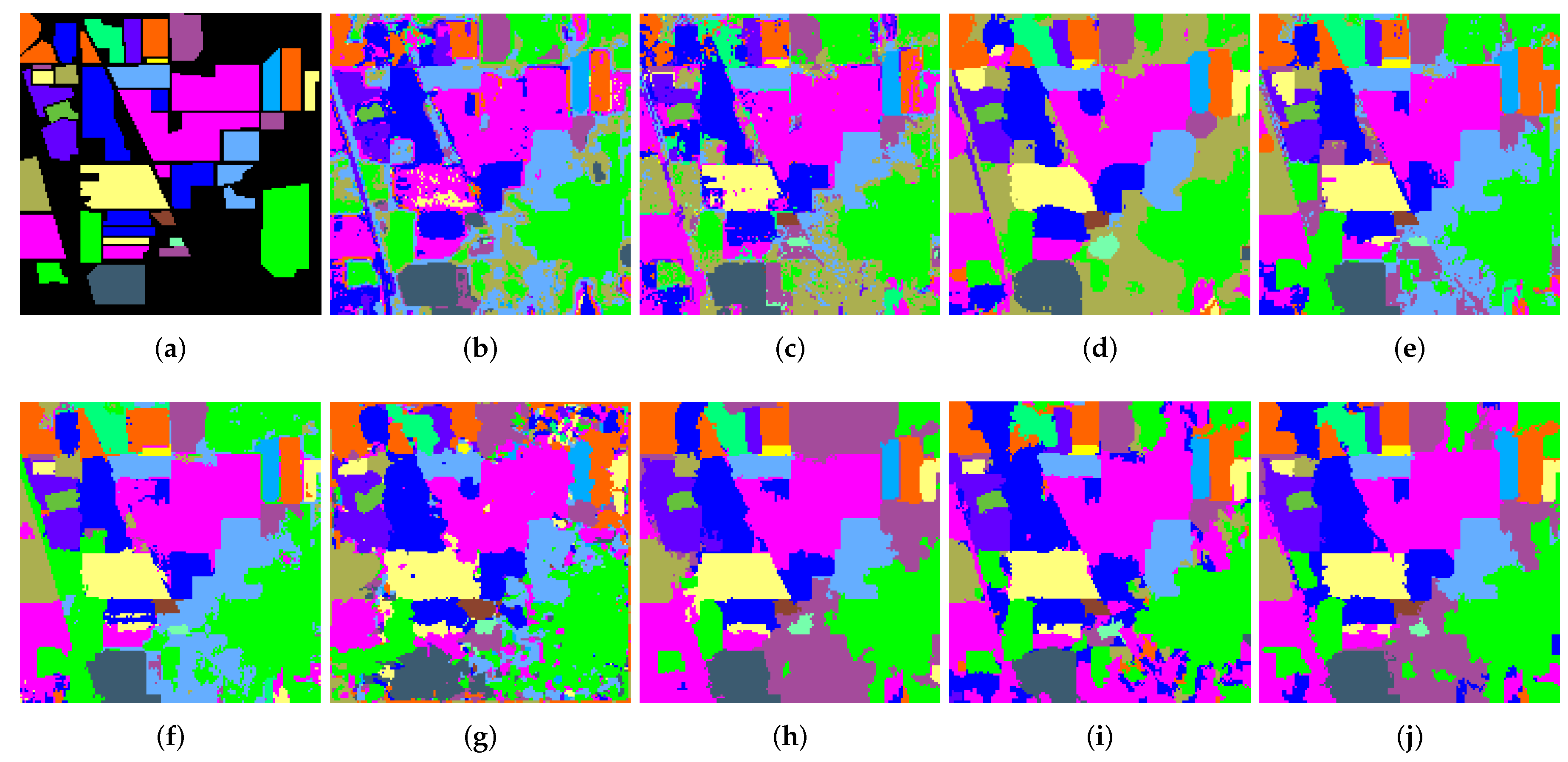
3.3. Classification Results

The classification results of all methods on the IP dataset are shown in Figure 2. Clearly, with the limited training samples, the proposed MASEMAP-MKL maintains the best object boundaries and detailed information of the image edge. The insufficient description of spatial information results in the methods based on SVM and CK giving the worst classification map. The SpMK method and the non-local similarity-based method SSK achieve better preservation of object boundaries only when they have enough training samples. Serious over-smoothing occurs in the classification map given by the EMAP, and the AIP method fails to accurately classify the marginal part of the categories. With the limited number of training samples, their ability to maintain better image details were inferior to that of the MASEMAP-MKL. However, a comparison with the ground-truth reveals that the proposed MASEMAP-MKL gives a classification map much closer to the ground-truth. Using adjacent superpixel segments and low-rank induced components, AMSSK and LRCISSSK further improve the ability to maintain image edges.

Compared with the latest methods, one certain conclusion is that the proposed MASEMAP-MKL achieved state-of-the-art classification results on the IP dataset, whose ground-truth distribution is relatively simple. Similar conclusions can be drawn from the classification results on the UP dataset, which has a more complex objective distribution. The classification maps are shown in Figure 3. The proposed method achieves the most accurate classification of the pixels located at the object boundaries, with the finest image texture. Another clear conclusion is that the advantages of the proposed method MASEMAP-MKL are further highlighted for more intricate images. The ability of our design to fully utilize spatial-spectral information is proven.

3.4. Classification Accuracy

The classification accuracy values of all methods on the IP and UP datasets are shown in

Table 2. Average classification accuracy (%) of all methods on the Indian Pines dataset with 2.7% labeled samples per class (the optimal results are highlighted in bold).

Categories	SVMCK [63]	SpMK [64]	ANSSK [54]	RMK [66]	EMAP [60]	AIP [65]	ASMSSK [52]	LRCISSK [55]	MASEMAP-MKL
1	19.01	80.00	95.58	94.81	95.97	58.65	97.12	97.12	100.00
2	83.15	85.60	96.15	94.89	62.59	74.41	96.78	96.61	98.64
3	81.44	78.52	95.35	94.23	75.12	66.67	98.62	97.10	99.26
4	34.63	62.82	96.87	84.41	76.75	68.90	91.06	91.94	97.80
5	85.26	86.50	87.83	90.66	79.41	63.02	94.62	90.43	99.79
6	95.99	96.46	97.01	98.66	94.34	70.08	98.46	97.43	98.06
7	10.00	95.83	97.08	96.25	92.31	81.25	95.42	95.83	100.00
8	97.50	98.36	99.47	99.24	93.20	80.29	99.79	99.90	100.00
9	0.00	98.89	90.56	100.00	100.00	67.78	99.44	96.67	100.00
10	29.43	76.31	86.97	86.80	77.70	53.12	89.42	84.65	92.14
11	90.34	89.87	97.68	97.77	70.86	79.13	98.72	97.75	98.04
12	73.81	59.18	94.99	92.39	70.89	60.67	98.18	93.32	97.50
13	94.80	99.31	99.22	99.51	98.03	70.05	99.02	99.36	99.02
14	96.48	95.93	99.72	99.63	78.76	81.02	99.22	99.49	98.73
15	61.95	74.09	96.12	96.48	70.15	77.67	96.26	95.18	98.65
16	88.02	81.10	95.38	96.26	90.71	69.34	94.84	96.15	92.31
OA(%)	80.11	85.63	95.84	95.41	75.69	72.11	97.12	95.76	97.90
std (%)	1.54	1.13	1.07	0.89	1.67	1.33	1.05	0.68	1.02
AA (%)	63.94	84.92	95.37	95.12	82.92	70.13	96.69	95.56	98.12
std (%)	1.94	1.59	1.70	0.89	0.54	2.34	0.99	0.85	0.96
Kappa	0.7702	0.8357	0.9525	0.9477	0.7256	0.6816	0.9672	0.9517	0.9761
std	0.0187	0.0129	0.0122	0.0102	0.0177	0.0153	0.0120	0.0078	0.0110

and

Table 3. Average classification accuracy (%) of all methods on the University of Pavia image with 15 labeled samples per class (the optimal results are highlighted in bold).

Categories	SVMCK [63]	SpMK [64]	ANSSK [54]	RMK [66]	EMAP [60]	AIP [65]	ASMSSK [52]	LRCISSK [55]	MASEMAP-MKL
1	83.02	90.08	89.83	94.76	86.60	84.28	96.60	96.21	93.49
2	82.91	80.87	86.07	91.07	74.12	85.61	93.60	89.79	98.66
3	78.97	91.47	81.81	95.55	92.71	85.18	99.51	92.62	99.74
4	93.10	81.22	88.03	89.18	91.14	80.93	89.22	90.43	88.32
5	99.02	98.87	96.92	98.85	97.18	99.56	98.68	99.44	98.57
6	81.67	93.89	96.85	92.68	81.39	95.28	97.94	98.86	96.97
7	89.63	99.47	96.88	97.55	97.94	94.03	98.94	98.87	99.24
8	76.32	92.20	91.44	93.21	90.88	73.31	98.22	98.33	98.69
9	98.42	81.26	99.36	88.73	99.57	99.25	97.44	91.04	98.44
OA (%)	83.80	86.49	89.28	92.49	82.49	86.12	95.36	94.62	96.99
std (%)	3.01	4.18	2.86	2.93	2.90	2.35	3.41	3.58	1.04
AA (%)	87.01	89.92	91.91	93.51	90.17	88.60	96.68	95.07	96.90
std (%)	1.28	2.16	1.13	1.45	2.54	1.45	1.28	2.23	0.62
Kappa	0.7913	0.8290	0.8616	0.9028	0.7778	0.8206	0.9397	0.9140	0.9601
std	0.0355	0.0499	0.0345	0.0368	0.0351	0.0289	0.0432	0.0428	0.0138

, respectively. The optimal values are highlighted in bold. Ten Monte Carlo runs were executed to obtain the average value. In almost all categories, the proposed MASEMAP-MKL achieved the highest accuracy. On the IP dataset, several categories achieved 100% classification accuracy. Meanwhile, the optimal OA, AA, and Kappa values were also obtained. On the UP dataset, which contained more complicated ground objectives, many competitors failed to maintain the balance between smoothness and fineness: the details of the image were lost, thus leading to inferior classification accuracy. The proposed method still achieved the optimal OA, AA, and Kappa values, which indicates that MASEMAP-MKL is more competitive on high spatial resolution images. Furthermore, the proposed MASEMAP-MKL also achieved the most stable std value for both OA and AA indicators. The results also show that the SSK-based method achieved higher classification accuracy than other competitors. The multiscale features-based method ASMSSK and the low-rank property-based method LRCISSSK achieved average second-best results compared with the proposed MASEMAP-MKL classifier. Thus, the advantages of fusing the multiscale features and multimodal features are reflected. In summary, the results of the above quantitative analysis demonstrate the effectiveness of the proposed method.

4. Discussion

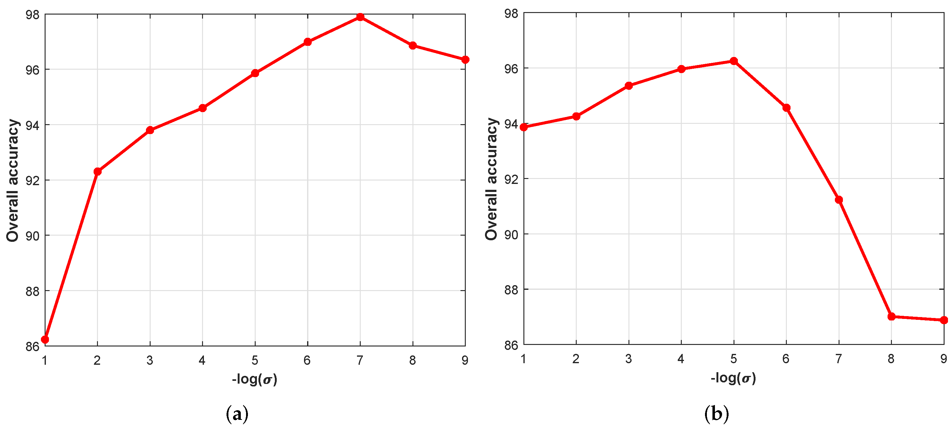
4.1. Parameter Analysis

The width of the kernel $\sigma$ plays a key role in classification. Figure 4 shows the classification accuracy of the proposed MASEMAP-MKL under different settings of $-log\left(\sigma \right)$ values on both the IP and UP datasets. On the IP dataset, when the $-log\left(\sigma \right)$ value was selected in the interval [5, 9], the proposed MASEMAP-MKL method achieved the highest classification accuracy. On the UP dataset, the value of $-log\left(\sigma \right)$ was selected in the interval [3, 6]. Therefore, we recommend choosing the kernel width parameter $-log\left(\sigma \right)$ according to the dataset itself.

4.2. Execution Efficiency

The execution efficiency of an algorithm determines its practicality in real scenarios.

Table 4. Execution time (seconds) of different classifiers on the IP and UP datasets (the optimal results are shown in bold).

	IP				UP
Classifiers	SpMK	ANSSK	ASMSSK	MASEMAP-MKL	SpMK	ANSSK	ASMSSK	MASEMAP-MKL
search similar regions	6.21	9.22	0.38	0.41	58.23	84.85	4.51	5.05
kernel computation	17.59	12.50	4.61	4.68	495.17	232.33	59.06	65.55
total	23.80	21.74	4.99	5.09	553.40	318.28	63.57	70.60

lists the average execution time of the proposed MASEMAP-MKL and three SSK-based methods in seconds. Each method was executed ten times to obtain the average value. For the SSK-based methods, the main computational cost was composed of two parts. The first part was the search of similar regions, and for this, ANSSK consumed the most time. This is because a non-local algorithm requires tedious block-matching and aggregation operations. With the assistance of the highly efficient superpixel division, both ASMSSK and MASEMAP-MKL achieved competitive time consumption for the search. The second part is the kernel computations. Because the HSI contained many pixels, both SpMK and ANSSK consumed an extremely high computing time. Meanwhile, The superpixels replaced the original pixels in our design, so the number of superpixels was much lower than the number of original pixels; therefore, both AMSSK and MASEMAP-MKL achieved a low kernel calculation cost. As the number of pixels increased, this advantage of the proposed method became more and more obvious. Although the time consumed by the proposed MASEMAP-MKL was slightly higher than that of the ASMSSK method, MASEMAP-MKL also achieved higher classification accuracy. The conclusion drawn is that our method achieves a better trade-off between efficiency and classification accuracy.

5. Conclusions and Future Work

To improve the accuracy and efficiency of HSI classification, a novel multiscale adjacent superpixel-based extended morphological attribute profile embedded multiple kernel learning method was proposed in this study. In summary, multiscale and multimodal spatial-spectral features are described by superpixel segmentation and the EMAP to construct different kernel functions. Meanwhile, we employed a PCA-based multi-kernel learning method to determine the weight of the different kernels. With our careful design, multiscale and multimodal features were fused, which makes full utilization of the ample spatial-spectral features for HSI classification. Extensive experiments on two datasets proved that the proposed method was both effective and efficient.

For future work, the fusion of deep features, multiscale features, and multimodal features will be considered to further improve the accuracy of HSI classification.

References

1. Zhong, S.; Chang, C.; Li, J.; Shang, X.; Chen, S.; Song, M.; Zhang, Y. Class feature weighted hyperspectral image classification. IEEE J. Sel. Top. Appl. Earth Obs. Remote Sens. 2019, 12, 4728–4745. [Google Scholar] [CrossRef]
2. Chen, Y.; Jiang, H.; Li, C.; Jia, X.; Ghamisi, P. Deep feature extraction and classification of hyperspectral images based on convolutional neural networks. IEEE Trans. Geosci. Remote Sens. 2016, 54, 6232–6251. [Google Scholar] [CrossRef] [Green Version]
3. Yu, C.; Zhao, M.; Song, M.; Wang, Y.; Li, F.; Han, R.; Chang, C. Hyperspectral image classification method based on CNN architecture embedding with hashing semantic feature. IEEE J. Sel. Top. Appl. Earth Obs. Remote Sens. 2019, 12, 1866–1881. [Google Scholar] [CrossRef]
4. Acosta, I.C.C.; Khodadadzadeh, M.; Tusa, L.; Ghamisi, P.; Gloaguen, R. A machine learning framework for drill-core mineral mapping using hyperspectral and high-resolution mineralogical data fusion. IEEE J. Sel. Top. Appl. Earth Obs. Remote Sens. 2019, 12, 4829–4842. [Google Scholar] [CrossRef]
5. Cao, Y.; Mei, J.; Wang, Y.; Zhang, L.; Peng, J.; Zhang, B.; Li, L.; Zheng, Y. SLCRF: Subspace learning with conditional random field for hyperspectral image classification. IEEE Trans. Geosci. Remote. Sens. 2020, 1–15. [Google Scholar] [CrossRef]
6. Yan, L.; Fan, B.; Liu, H.; Huo, C.; Xiang, S.; Pan, C. Triplet adversarial domain adaptation for pixel-level classification of VHR remote sensing images. IEEE Trans. Geosci. Remote Sens. 2019, 58, 3558–3573. [Google Scholar] [CrossRef]
7. Zhang, X.; Peng, F.; Long, M. Robust coverless image steganography based on DCT and LDA topic classification. IEEE Trans. Multimed. 2018, 20, 3223–3238. [Google Scholar] [CrossRef]
8. Chen, Y.; Xu, W.; Zuo, J.; Yang, K. The fire recognition algorithm using dynamic feature fusion and IV-SVM classifier. Clust. Comput. 2019, 22, 7665–7675. [Google Scholar] [CrossRef]
9. Cui, H.; Shen, S.; Gao, W.; Liu, H.; Wang, Z. Efficient and robust large-scale structure-from-motion via track selection and camera prioritization. ISPRS J. Photogramm. Remote Sens. 2019, 156, 202–214. [Google Scholar] [CrossRef]
10. Song, Y.; Cao, W.; Shen, Y.; Yang, G. Compressed sensing image reconstruction using intra prediction. Neurocomputing 2015, 151, 1171–1179. [Google Scholar] [CrossRef]
11. Sun, L.; He, C.; Zheng, Y.; Tang, S. SLRL4D: Joint restoration of subspace low-rank learning and non-local 4-d transform filtering for hyperspectral image. Remote Sens. 2020, 12, 2979. [Google Scholar] [CrossRef]
12. Song, Y.; Yang, G.; Xie, H.; Zhang, D.; Xingming, S. Residual domain dictionary learning for compressed sensing video recovery. Multimed. Tools Appl. 2017, 76, 10083–10096. [Google Scholar] [CrossRef]
13. Tu, B.; Huang, S.; Fang, L.; Zhang, G.; Wang, J.; Zheng, B. Hyperspectral image classification via weighted joint nearest neighbor and sparse representation. IEEE J. Sel. Top. Appl. Earth Obs. Remote Sens. 2018, 11, 4063–4075. [Google Scholar] [CrossRef]
14. Peng, J.; Sun, W.; Du, Q. Self-paced joint sparse representation for the classification of hyperspectral images. IEEE Trans. Geosci. Remote Sens. 2019, 57, 1183–1194. [Google Scholar] [CrossRef]
15. Fang, L.; Li, S.; Kang, X.; Benediktsson, J.A. Spectral–spatial hyperspectral image classification via multiscale adaptive sparse representation. IEEE Trans. Geosci. Remote Sens. 2014, 52, 7738–7749. [Google Scholar] [CrossRef]
16. Dundar, T.; Ince, T. Sparse representation-based hyperspectral image classification using multiscale superpixels and guided filter. IEEE Geosci. Remote Sens. Lett. 2019, 16, 246–250. [Google Scholar] [CrossRef]
17. Jia, S.; Deng, X.; Zhu, J.; Xu, M.; Zhou, J.; Jia, X. Collaborative representation-based multiscale superpixel fusion for hyperspectral image classification. IEEE Trans. Geosci. Remote Sens. 2019, 57, 7770–7784. [Google Scholar] [CrossRef]
18. Yang, J.; Qian, J. Hyperspectral image classification via multiscale joint collaborative representation with locally adaptive dictionary. IEEE Geosci. Remote Sens. Lett. 2018, 15, 112–116. [Google Scholar] [CrossRef]
19. Ma, Y.; Li, C.; Li, H.; Mei, X.; Ma, J. Hyperspectral image classification with discriminative kernel collaborative representation and tikhonov regularization. IEEE Geosci. Remote Sens. Lett. 2018, 15, 587–591. [Google Scholar] [CrossRef]
20. Wang, Q.; He, X.; Li, X. Locality and structure regularized low rank representation for hyperspectral image classification. IEEE Trans. Geosci. Remote Sens. 2019, 57, 911–923. [Google Scholar] [CrossRef] [Green Version]
21. Wang, Y.; Mei, J.; Zhang, L.; Zhang, B.; Li, A.; Zheng, Y.; Zhu, P. Self-supervised low-rank representation (sslrr) for hyperspectral image classification. IEEE Trans. Geosci. Remote Sens. 2018, 56, 5658–5672. [Google Scholar] [CrossRef]
22. Ding, Y.; Chong, Y.; Pan, S. Sparse and low-rank representation with key connectivity for hyperspectral image classification. IEEE J. Sel. Top. Appl. Earth Obs. Remote Sens. 2020, 13, 5609–5622. [Google Scholar] [CrossRef]
23. Mei, S.; Hou, J.; Chen, J.; Chau, L.; Du, Q. Simultaneous spatial and spectral low-rank representation of hyperspectral images for classification. IEEE Trans. Geosci. Remote Sens. 2018, 56, 2872–2886. [Google Scholar] [CrossRef]
24. Wei, W.; Yongbin, J.; Yanhong, L.; Ji, L.; Xin, W.; Tong, Z. An advanced deep residual dense network (DRDN) approach for image super-resolution. Int. J. Comput. Intell. Syst. 2019, 12, 1592–1601. [Google Scholar] [CrossRef] [Green Version]
25. Fan, B.; Liu, H.; Zeng, H.; Zhang, J.; Liu, X.; Han, J. Deep unsupervised binary descriptor learning through locality consistency and self distinctiveness. IEEE Trans. Multimed. 2020. [Google Scholar] [CrossRef]
26. Zeng, D.; Dai, Y.; Li, F.; Wang, J.; Sangaiah, A.K. Aspect based sentiment analysis by a linguistically regularized CNN with gated mechanism. J. Intell. Fuzzy Syst. 2019, 36, 3971–3980. [Google Scholar] [CrossRef]
27. Zhang, J.; Jin, X.; Sun, J.; Wang, J.; Sangaiah, A.K. Spatial and semantic convolutional features for robust visual object tracking. Multimed. Tools Appl. 2020, 79, 15095–15115. [Google Scholar] [CrossRef]
28. Hong, D.; Gao, L.; Yokoya, N.; Yao, J.; Chanussot, J.; Du, Q.; Zhang, B. More diverse means better: Multimodal deep learning meets remote-sensing imagery classification. IEEE Trans. Geosci. Remote. Sens. 2020, 1–15. [Google Scholar] [CrossRef]
29. Hong, D.; Yokoya, N.; Chanussot, J.; Zhu, X.X. An augmented linear mixing model to address spectral variability for hyperspectral unmixing. IEEE Trans. Image Process. 2018, 28, 1923–1938. [Google Scholar] [CrossRef] [Green Version]
30. Wang, J.; Song, X.; Sun, L.; Huang, W.; Wang, J. A novel cubic convolutional neural network for hyperspectral image classification. IEEE J. Sel. Top. Appl. Earth Obs. Remote Sens. 2020, 13, 4133–4148. [Google Scholar] [CrossRef]
31. Lu, Z.; Xu, B.; Sun, L.; Zhan, T.; Tang, S. 3-D Channel and spatial attention based multiscale spatial–spectral residual network for hyperspectral image classification. IEEE J. Sel. Top. Appl. Earth Obs. Remote Sens. 2020, 13, 4311–4324. [Google Scholar] [CrossRef]
32. Liu, P.; Zhang, H.; Eom, K.B. Active deep learning for classification of hyperspectral images. IEEE J. Sel. Top. Appl. Earth Obs. Remote Sens. 2017, 10, 712–724. [Google Scholar] [CrossRef] [Green Version]
33. Zhong, P.; Gong, Z.; Li, S.; Schönlieb, C.B. Learning to diversify deep belief networks for hyperspectral image classification. IEEE Trans. Geosci. Remote Sens. 2017, 55, 3516–3530. [Google Scholar] [CrossRef]
34. Haut, J.M.; Paoletti, M.E.; Plaza, J.; Li, J.; Plaza, A. Active learning with convolutional neural networks for hyperspectral image classification using a new bayesian approach. IEEE Trans. Geosci. Remote Sens. 2018, 56, 6440–6461. [Google Scholar] [CrossRef]
35. Yang, X.; Ye, Y.; Li, X.; Lau, R.Y.K.; Zhang, X.; Huang, X. Hyperspectral image classification with deep learning models. IEEE Trans. Geosci. Remote Sens. 2018, 56, 5408–5423. [Google Scholar] [CrossRef]
36. Zhu, L.; Chen, Y.; Ghamisi, P.; Benediktsson, J.A. Generative adversarial networks for hyperspectral image classification. IEEE Trans. Geosci. Remote Sens. 2018, 56, 5046–5063. [Google Scholar] [CrossRef]
37. Zhan, Y.; Hu, D.; Wang, Y.; Yu, X. Semisupervised hyperspectral image classification based on generative adversarial networks. IEEE Geosci. Remote Sens. Lett. 2018, 15, 212–216. [Google Scholar] [CrossRef]
38. Chen, Y.; Wang, J.; Xia, R.; Zhang, Q.; Cao, Z.; Yang, K. The visual object tracking algorithm research based on adaptive combination kernel. J. Ambient Intell. Humaniz. Comput. 2019, 10, 4855–4867. [Google Scholar] [CrossRef]
39. Liu, H.; Zhang, Q.; Fan, B.; Wang, Z.; Han, J. Features combined binary descriptor based on voted ring-sampling pattern. IEEE Trans. Circuits Syst. Video Technol. 2020, 30, 3675–3687. [Google Scholar] [CrossRef]
40. Zhan, T.; Sun, L.; Xu, Y.; Wan, M.; Wu, Z.; Lu, Z.; Yang, G. Hyperspectral classification using an adaptive spectral-spatial kernel-based low-rank approximation. Remote Sens. Lett. 2019, 10, 766–775. [Google Scholar] [CrossRef]
41. Gu, Y.; Chanussot, J.; Jia, X.; Benediktsson, J.A. Multiple kernel learning for hyperspectral image classification: A review. IEEE Trans. Geosci. Remote Sens. 2017, 55, 6547–6565. [Google Scholar] [CrossRef]
42. Zhan, T.; Sun, L.; Xu, Y.; Yang, G.; Zhang, Y.; Wu, Z. Hyperspectral classification via superpixel kernel learning-based low rank representation. Remote Sens. 2018, 10, 1639. [Google Scholar] [CrossRef] [Green Version]
43. Sun, Y.; Zhang, X. Composite kernel classification using spectral-spatial features and abundance information of hyperspectral image. In Proceedings of the 2018 9th Workshop on Hyperspectral Image and Signal Processing: Evolution in Remote Sensing (WHISPERS), Amsterdam, The Netherlands, 23–26 September 2018; pp. 1–5. [Google Scholar]
44. Jin, X.; Gu, Y. Combine reflectance with shading component for hyperspectral image classification. In Proceedings of the IGARSS 2018—2018 IEEE International Geoscience and Remote Sensing Symposium, Valencia, Spain, 22–27 July 2018; pp. 9–12. [Google Scholar]
45. Chen, P. Hyperspectral image classification based on broad learning system with composite feature. In Proceedings of the 2020 IEEE International Conference on Power, Intelligent Computing and Systems (ICPICS), Shenyang, China, 28–30 July 2020; pp. 842–846. [Google Scholar]
46. Chen, Y.; Xiong, J.; Xu, W.; Zuo, J. A novel online incremental and decremental learning algorithm based on variable support vector machine. Clust. Comput. 2019, 22, 7435–7445. [Google Scholar] [CrossRef]
47. Huang, H.; Duan, Y.; Shi, G.; Lv, Z. Fusion of weighted mean reconstruction and svmck for hyperspectral image classification. IEEE Access 2018, 6, 15224–15235. [Google Scholar] [CrossRef]
48. Duan, P.; Kang, X.; Li, S.; Ghamisi, P.; Benediktsson, J.A. Fusion of multiple edge-preserving operations for hyperspectral image classification. IEEE Trans. Geosci. Remote Sens. 2019, 57, 10336–10349. [Google Scholar] [CrossRef]
49. Tajiri, K.; Maruyama, T. FPGA acceleration of a supervised learning method for hyperspectral image classification. In Proceedings of the 2018 International Conference on Field-Programmable Technology (FPT), Naha, Japan, 10–14 December 2018; pp. 270–273. [Google Scholar]
50. Hong, D.; Yokoya, N.; Ge, N.; Chanussot, J.; Zhu, X.X. Learnable manifold alignment (LeMA): A semi-supervised cross-modality learning framework for land cover and land use classification. ISPRS J. Photogramm. Remote Sens. 2019, 147, 193–205. [Google Scholar] [CrossRef] [PubMed]
51. Dong, Y.; Liang, T.; Zhang, Y.; Du, B. Spectral-spatial weighted kernel manifold embedded distribution alignment for remote sensing image classification. IEEE Trans. Cybern. 2020, 1–13. [Google Scholar] [CrossRef]
52. Sun, L.; Ma, C.; Chen, Y.; Shim, H.J.; Wu, Z.; Jeon, B. Adjacent superpixel-based multiscale spatial-spectral kernel for hyperspectral classification. IEEE J. Sel. Top. Appl. Earth Obs. Remote Sens. 2019, 12, 1905–1919. [Google Scholar] [CrossRef]
53. Yang, H.L.; Zhang, Y.; Prasad, S.; Crawford, M. Multiple kernel active learning for robust geo-spatial image analysis. In Proceedings of the 2013 IEEE International Geoscience and Remote Sensing Symposium-IGARSS, Melbourne, Australia, 21–26 July 2013; IEEE: Piscataway, NJ, USA, 2013; pp. 1218–1221. [Google Scholar]
54. Wang, J.; Jiao, L.; Wang, S.; Hou, B.; Liu, F. Adaptive nonlocal spatial–spectral kernel for hyperspectral imagery classification. IEEE J. Sel. Top. Appl. Earth Obs. Remote Sens. 2016, 9, 4086–4101. [Google Scholar] [CrossRef]
55. Sun, L.; Ma, C.; Chen, Y.; Zheng, Y.; Shim, H.J.; Wu, Z.; Jeon, B. Low rank component induced spatial-spectral kernel method for hyperspectral image classification. IEEE Trans. Circuits Syst. Video Technol. 2020, 30, 3829–3842. [Google Scholar] [CrossRef]
56. Wang, Q.; Gu, Y.; Tuia, D. Discriminative multiple kernel learning for hyperspectral image classification. IEEE Trans. Geosci. Remote Sens. 2016, 54, 3912–3927. [Google Scholar] [CrossRef]
57. Li, F.; Lu, H.; Zhang, P. An innovative multi-kernel learning algorithm for hyperspectral classification. Comput. Electr. Eng. 2019, 79, 106456. [Google Scholar] [CrossRef]
58. Li, D.; IEEE, Q.W.M.; Kong, F. Superpixel-feature-based multiple kernel sparse representation for hyperspectral image classification. Signal Process. 2020, 2020, 107682. [Google Scholar] [CrossRef]
59. Achanta, R.; Shaji, A.; Smith, K.; Lucchi, A.; Fua, P.; SAsstrunk, S. SLIC superpixels compared to state-of-the-art superpixel methods. IEEE Trans. Pattern Anal. Mach. Intell. 2012, 34, 2274–2282. [Google Scholar] [CrossRef] [Green Version]
60. Dalla Mura, M.; Villa, A.; Benediktsson, J.A.; Chanussot, J.; Bruzzone, L. Classification of hyperspectral images by using extended morphological attribute profiles and independent component analysis. IEEE Geosci. Remote Sens. Lett. 2011, 8, 542–546. [Google Scholar] [CrossRef] [Green Version]
61. Peeters, S.; Marpu, P.R.; Benediktsson, J.A.; Dalla Mura, M. Classification using extended morphological sttribute profiles based on different feature extraction techniques. In Proceedings of the 2011 IEEE International Geoscience and Remote Sensing Symposium, Vancouver, BC, Cananda, 24–29 July 2011; pp. 4453–4456. [Google Scholar]
62. Song, B.; Li, J.; Li, P.; Plaza, A. Decision fusion based on extended multi-attribute profiles for hyperspectral image classification. In Proceedings of the 2013 5th Workshop on Hyperspectral Image and Signal Processing: Evolution in Remote Sensing (WHISPERS), Gainesville, FL, USA, 25–28 June 2013; pp. 1–4. [Google Scholar]
63. Camps-Valls, G.; Gomez-Chova, L.; Muñoz-Marí, J.; Vila-Francés, J.; Calpe-Maravilla, J. Composite kernels for hyperspectral image classification. IEEE Geosci. Remote Sens. Lett. 2006, 3, 93–97. [Google Scholar] [CrossRef]
64. Fang, L.; Li, S.; Duan, W.; Ren, J.; Benediktsson, J.A. Classification of hyperspectral images by exploiting spectral–spatial information of superpixel via multiple kernels. IEEE Trans. Geosci. Remote Sens. 2015, 53, 6663–6674. [Google Scholar] [CrossRef] [Green Version]
65. Hong, D.; Wu, X.; Ghamisi, P.; Chanussot, J.; Yokoya, N.; Zhu, X. Invariant attribute profiles: A spatial-frequency joint feature extractor for hyperspectral image classification. IEEE Trans. Geosci. Remote Sens. 2020, 58, 3791–3808. [Google Scholar] [CrossRef] [Green Version]
66. Liu, J.; Wu, Z.; Xiao, Z.; Yang, J. Region-based relaxed multiple kernel collaborative representation for hyperspectral image classification. IEEE Access 2017, 5, 20921–20933. [Google Scholar] [CrossRef]
Figure 1. Flowchart of the proposed multiscale, adjacent superpixel-based embedded multiple kernel learning method with the extended multi-attribute profile (MASEMAP-MKL) method.
Remotesensing 13 00050 g001
Figure 2. Classification results of Indian Pines (IP) with about 2.7% training samples per class. (a) Ground-truth; (b) SVM-CK; (c) SpMK; (d) ANSSK; (e) RMK; (f) EMAP; (g) invariant attribute profile (AIP); (h) ASMSSK; (i) LRCISSK; (j) MASEMAP-MKL.
Remotesensing 13 00050 g002
Figure 3. Classification results of University of Pavia (UP) with 15 training samples per class. (a) Ground-truth; (b) SVM-CK; (c) SpMK; (d) ANSSK; (e) RMK; (f) EMAP; (g) AIP; (h) ASMSSK; (i) LRCISSK; (j) MASEMAP-MKL.
Remotesensing 13 00050 g003
Figure 4. Classification accuracies of the proposed MASEMAP-MKL method as a function of parameter σ : (a) IP; (b) UP.
Remotesensing 13 00050 g004