Abstract
The study deals with the application of Google Earth Engine (GEE), Landsat data and ensemble-learning methods (ELMs) to map land cover (LC) change over a decade in the Kaski district of Nepal. As Nepal has experienced extensive changes due to natural and anthropogenic activities, monitoring such changes are crucial for understanding relationships and interactions between social and natural phenomena and to promote better decision-making. The main novelty lies in applying the XGBoost classifier for LC mapping over Nepal and monitoring the decadal changes of LC using ELMs. To map the LC change, a yearly cloud-free composite Landsat image was selected for the year 2010 and 2020. Combining the annual normalized difference vegetation index, normalized difference built-up index and modified normalized difference water index, with elevation and slope data from shuttle radar topography mission, supervised classification was performed using a random forest and extreme gradient boosting ELMs. Post classification change detection, validation and accuracy assessment were executed after the preparation of the LC maps. Three evaluation indices, namely overall accuracy (OA), Kappa coefficient, and F1 score from confusion matrix reports, were calculated for all the points used for validation purposes. We have obtained an OA of 0.8792 and 0.875 for RF and 0.8926 and 0.8603 for XGBoost at the 95% confidence level for 2010 and 2020 LC maps, which are better for mountainous terrain. The applied methodology could be significant in utilizing the big earth observation data and overcoming the traditional computational challenges using GEE. In addition, the quantification of changes over time would be helpful for decision-makers to understand current environmental dynamics in the study area.
1. Introduction
Nepal, a seismically active [1] and economically developing country [2], lies between India and China. In 2015, Nepal experienced a massive earthquake and many aftershocks destroying many infrastructures and lives [3,4,5]. In the past decade, Nepal has seen rapid population growth and unplanned urbanization leading to many infrastructure developments from rural excavated roads to national highway projects [4,6]. Many forest areas were converted to cultivation lands, and existing cultivation lands were converted to built-up areas. These alterations are causing undulations in river courses and patterns, thus further affecting the water quantity and quality of rivers [7,8,9,10,11]. All these natural and anthropogenic activities have altered the land cover (LC) rapidly in Nepal. Regular LC mapping and change detection is an utmost important task to maintain pace with these changes. Regular monitoring of LC change through an updated database helps us access global climatic pattern change and mitigate its issues [12]. LC changes are crucial for understanding relationships and interactions between human and natural phenomena and to promote better decision-making for sustainable development [13].
Earth observation (EO) data are one of the best resources for measuring LC dynamics [14,15,16]. It started with the Landsat satellite mission launch and has been continuously monitoring the earth’s surface for more than four decades [17,18,19]. While many satellites with advanced capabilities have been launched for the same purpose, Landsat has continuously evolved, with each mission maintaining its legacy. This vast collection of data is also freely available for researchers, which is a great asset to the scientific community. Many case studies have been conducted for LC mapping and change detection [20,21,22,23,24,25,26,27]. Many indices have been developed to extract a single feature, whereas recent advancements in machine learning (ML) algorithms have significantly improved classification accuracy [28,29,30,31,32]. However, working on multiple satellite imageries/scenes in edge devices is tedious, time-consuming and often requires enormous storage space. One possible approach to handle such massive EO data for large spatial and temporal extents is to utilize multiple computers, which is also an expensive investment for a few times of use. An optimum solution that could solve all the above problems would be a cloud-based public computing platform. This conserves the infrastructure, cost, computing time and maximum utilization issues at one step. Google Earth Engine (GEE) is such a cloud-based computing platform that has a vast amount of satellite data. GEE makes satellite imagery processing very convenient [33,34,35]. This method provides free and easy data access and analyzes the massive amount of data in a matter of seconds. Some previous works in Asia, China, Africa, and the USA have shown a promising use of GEE [34,35,36,37,38,39,40,41].
Though there are many conventional methods for mapping LC and its dynamics, these processes are time-consuming and require much computational power. To overcome these limitations, one possible solution is the implementation of ML algorithms that not only provide efficient computing performance in terms of power and time but also furnish more accurate results than conventional methods. With the advancement in computing technology, many studies have been conducted by combining statistical methods with machine learning models such as artificial neural networks (ANN), logistic regression (LR), decision trees (DT) and support vector machines (SVM) and has been reported to perform better than conventional methods [42,43,44]. Accuracy can be furthermore enhanced using the ensemble-learning methods (ELMs) that combine several models to one predictive model that decreases variance (bagging), bias (boosting) and improves predictions (stacking) that produces better accuracy than a single ML model [45,46]. Many studies have proved the significance of the ensemble model over a single and conventional model [42,47,48,49]. Random forest (RF) and extreme gradient boosting (XGBoost) are some of the models based on an algorithm of ensemble methods.
From the aforementioned literature, it can be observed that EO data can act as an alternative to traditional data acquisition and machine learning algorithms are more advanced than traditional supervised and unsupervised classifiers. To test their applicability for mountainous terrain, we have implemented GEE and ELMs for LC mapping of mountainous terrain in Nepal, i.e., the Kaski district. The main novelty lies in applying the XGBoost classifier for LC mapping over Nepal and monitoring the decadal changes of LC using ELMs for mountainous terrain. The main objectives of the current research are:
- To acquire the median composite imagery and their three derivative indices for the years 2010 and 2020 using GEE;
- To map and evaluate the accuracies of the LC changes using RF and XGBoost ELMs;
- To compare the accuracy and identify the best performing method for mapping LC;
- To quantify and validate the LC changes in Kaski District, Nepal.
The applied methodology is a case study for the hilly region of Nepal. The methodology can be an essential adoption in developing countries like Nepal to utilize big EO data and overcome the computational challenges. In addition, the quantification of LC and changes over time would be helpful for decision-makers to understand current environmental dynamics. Figure 1 depicts the workflow adopted for the LC classification and change detection in this study.
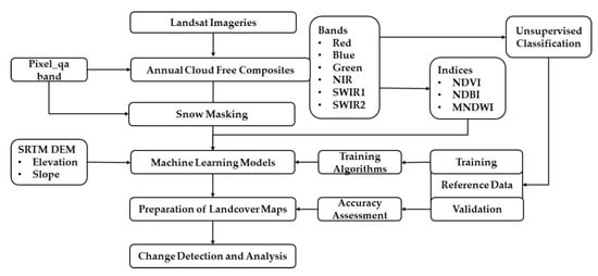
Figure 1.
The workflow adopted for the land cover (LC) classification and change detection in this study.
2. Study Area and Data
2.1. Study Area
The Kaski district lies between 28°4′35″–28°36′44″ N latitude and 83°42′10.53″–84°16′49″ E longitude in Province 5 of Nepal. It has the second largest metropolitan city of Nepal, Pokhara, which experienced tremendous urbanization in the past decade [50]. Pokhara is a primary tourist attraction site and one of the significant economic hubs of Nepal. This district represents Nepal geographically as it has the snow-covered Annapurna mountain range, three major lakes, one of the biggest valleys and many rivers. Most of the area of the LC of the Kaski district is occupied by forest and cultivation areas. The snow-covered area is also prominent in the Kaski district. The study area is shown in Figure 2.
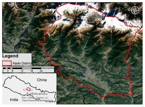
Figure 2.
Location map of the Kaski district, Nepal, with natural color cloud-free Landsat composite.
2.2. Data
2.2.1. Satellite Data
In this study, all the datasets used are available from the GEE repository. GEE provides atmospherically corrected, tier 1 surface reflectance imagery along with many other datasets. Landsat 5 and 8 were used for the years 2010 and 2020 for LC change mapping. Table 1 shows the band combination of Landsat 5 and 8 data. Both satellites have sun-synchronous orbit and have a temporal resolution of 16 days. The data are available as approximately 185 km × 180 km scenes defined in a worldwide reference system (WRS) of the path and row coordinates [51,52]. Landsat 5 data were atmospherically corrected using Landsat ecosystem disturbance adaptive processing system (LEDAPS) [53]. Landsat 8 data were atmospherically corrected using land surface reflectance code (LaSRC) [54] that includes a cloud, shadow, water and snow mask produced using the C function of Mask (CFMASK) [55], as well as a per-pixel saturation mask.

Table 1.
The bands, ranges and names of Landsat 5 and Landsat 8 data.
Since Nepal’s Kaski district is a cloudy area, most of the Kaski district areas lie in the cloud covered portion of Landsat images. Hence, obtaining a full scene without a cloud of the same day or month is challenging. Hence, we performed cloud masking in the scene and applied median filtering to the scene to get smooth and continuous coverage of the scene without clouds resulting in the annual median composite.
In addition to surface reflectance, the slope was also used to aid the classification. The slope was derived from the shuttle radar topography mission (SRTM), an international research effort that obtained a digital elevation model (DEM) on a near-global scale [56]. This SRTM V3 product (SRTM Plus) is provided by National Aeronautics Space Administration Jet Propulsion Laboratory at a resolution of 1 arc-second (approximately 30 m) [57]. This dataset has undergone a gap-filling process using open-source data (ASTER GDEM2, GMTED2010 and NED) instead of other versions that contain voids or were gap-filled with commercial sources. Dem helps to eliminate the confusion created by the shadow of terrain as it has similar spectral characteristics to water in the optical image. Figure 3 shows the map representing elevation and slope from SRTM dem. The elevation of the Kaski district ranges from 450 m to 8091 m.
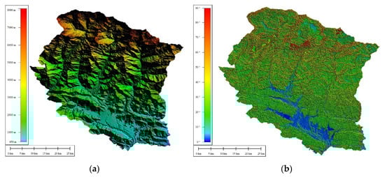
Figure 3.
Maps obtained from shuttle radar topography mission (SRTM) dem: (a) elevation; (b) slope.
2.2.2. Spectral Indices
Various spectral indices were derived from the primary bands of Landsat imagery. These bands in amalgamation with other primary bands were used as training data to produce the LC maps. These multiple indices help us classify images accurately, thereby reducing hillshade and building shadows. The adopted indices are:
- 1.
- NDVI is the normalized difference between the NIR band and the red band. NIR bands are more sensitive to vegetation [58] and are used to perceive the vegetation’s richness. It is calculated as shown in Equation (1).
- 2.
- NDBI is the normalized difference between SWIR1 and NIR bands [59,60]. It separates the built-up area from the background. It is calculated as shown in Equation (2).
- 2.
- MNDWI is the normalized difference between SWIR1 and green bands. It accurately segregates the water body mitigating the built-up noise [61]. It is calculated as shown in Equation (3).
2.2.3. LC Label Scheme
The cloud masking scheme in the preprocessing of Landsat data masked some of the permanent ice covering areas in the study area. This created voids and difficulty in the classification of the snow LC. To mitigate this problem, we masked out the snow area from the image and only the remaining portion of the image was used for the classification, thus resulting in only five labels out of six LC classes. The classes were determined according to the major classes from the Nepal government’s LC map. These classes overall represent the LC of the Kaski district. Table 2 shows the LC types classified in this study.
Table 2.
LC classes with labels in the reference dataset.
2.2.4. Reference Data
For this study, reference data were prepared in the area, leaving snow cover. First, the unsupervised classification was performed to understand the clustering of similar features. Based on the area coverage of unsupervised pixels, reference points were selected using stratified sampling. For each point, labels from Table 2 were added according to the same year high-resolution imagery available in Google Earth Pro. For a better representation of the area, the expert’s judgment was used to add and remove points. A total of 593 and 542 reference points for all LC classes (excluding snow) were collected for the images of 2010 and 2020, respectively, omitting the NA values. The reference data for the Landsat image from 2010 and 2020 are shown in Figure 4. Training and validation points were prepared by randomly splitting the data at 75% for 2020 and 80% for 2010.
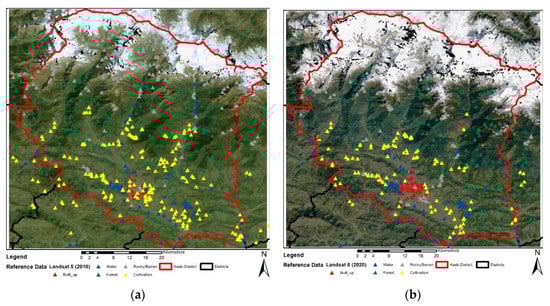
Figure 4.
Distribution of training data: (a) for the year 2010; (b) for the year 2020.
3. Methodology
First, reference data were prepared for the LC classification of the Kaski district during the years 2020 and 2010. For this purpose, unsupervised K-means classification was performed on the Landsat 8 and Landsat 5 imagery. A total of 50 clusters was made for the classification. The spectral similarity between the classes was observed. With the help of unsupervised clusters and the respective year’s google imagery, the reference data were prepared. Later the number of reference data was adjusted in proportional to the area of the ten unsupervised training classes. In GEE, a cloud-free composite of the Landsat 5 and Landsat 8 surface reflectance (SR) of the whole year was taken using the median filter for the composite. Cloud-free composites were made by masking out the clouds from the image. Snow masking was also performed to remove the void pixels from the image. The true- and false-color composites of the median Landsat SR are shown in Figure 5.
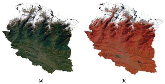
Figure 5.
Median composite of the clipped Landsat scenes of Kaski District for the year 2020. (a) True-color composite; (b) false-color composite.
Further, several indices like NDVI, NDBI and MNDWI were derived from the primary bands of satellite imagery. These bands were used to accurately classify the Landsat imagery eliminating shadows of hills and buildings. Since Kaski has a snow-covered Himalayan range and hills, topographical factors like slope and elevation obtained from SRTM DEM were also used for classification. The total reference data were randomly divided into a test set and a validation set. The yearly composite data were downloaded and further processed using the R programming language. The hyperparameter tuning was performed for both algorithms for both years, and the best hyperparameter was used for the LC mapping. Later, RF and XGBoost based classification was executed for the supervised classification. RF uses various carts as a single unit to give the best result. LC maps were generated for each test area using both compositing methods, and the classification accuracy of each map was computed using the corresponding validation data sets.
After preparing the LC classification in the R, postprocessing was done in ArcGIS Pro. The majority filter of eight neighborhood pixels was applied to remove the salt-and-pepper effect on the obtained maps. The changes were computed between RF-derived categorical classes for two years. Finally, post-classification change was detected and mapped. The change map was analyzed using Sankey’s diagram.
3.1. Ensemble Learning Methods
3.1.1. Random Forest Algorithm
Random forest (RF) is the ensemble of many relatively uncorrelated decision trees that operate as a single unit [62]. A decision tree is a simple (Figure 6), deterministic data structure for modeling decision rules for a specific classification problem. At each node, one feature is selected to make class determining the decision. Each tree in the ensemble is built from a sample drawn with replacement (i.e., a bootstrap sample) from the training set. It produces stable results without even the requirement of hyperparameter tuning. The RF algorithm was selected because of its robustness and accuracy. RF can process features with many dimensions, and it can use continuous and categorical data sets. RF is easy to parametrize, is not sensitive to over-fitting, and is even good at dealing with outliers in training data. RF even calculates ancillary information such as classification error and variable importance [62].
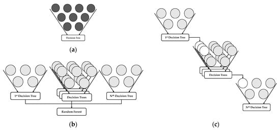
Figure 6.
Representation of models. (a) Single tree out of all samples; (b) bagging grows tree parallel with subsamples; (c) boosting grows tree sequentially with weighted samples.
3.1.2. Extreme Gradient Boosting Algorithm
Gradient Boosting Algorithm is the ELM, which builds the model in a stage-wise fashion as other boosting methods do (Figure 6), and it generalizes them by allowing optimization of an arbitrary differentiable loss function [63]. XGBoost is one of the implementations of the Gradient Boosting concept, but what makes XGBoost unique is that it uses more regularized model formalization for controlling overfitting and better model performance. Its execution speed is fast than other gradient boosting algorithms. The goal of this algorithm is to push the extreme of the computation limits of machines to provide a scalable, portable and accurate library. XGBoost not only eliminates biases but also removes variance in the result. It provides efficient handling of missing data and promotes tree pruning using a depth-free approach.
3.2. Accuracy Assessment
Training of our model was controlled using a 10-fold cross-validation (CV) method. An accuracy assessment was done using the validation data set. Three evaluation indices, namely the overall accuracy (OA), Kappa coefficient (Kappa) and F1 score from confusion matrix reports, were calculated for all the points used for validation purposes. OA determines the algorithm’s overall efficiency and can be calculated by dividing the total number of correctly labeled samples by the total number of the testing samples [64]. The Kappa indicates the degree of agreement between the ground truth data and the predicted values [65]. The F1 score was calculated from the precision and recall of the test, where the precision is the number of correctly identified positive results divided by the number of all positive results, including those not identified correctly. The recall is the number of correctly identified positive results divided by the number of all samples that should have been identified as positive [66,67]. The no-information rate (NIR) is the largest proportion of the observed classes. We also calculated producer accuracy for all the classes. The producer’s accuracy represents the probability that a reference sample is correctly identified in the classification map. Table 3 shows a representation of a confusion matrix for two classes:
OA = (A + C)/(A + B + C + D)
Recall = A/A + C
Precision = A/A + B
F1 score = (1 + β2)(precision ∗ recall)/(β2 ∗ precision + recall)
Table 3.
Confusion matrix for 2 × 2 matrix.
Suppose that there is response yi and covariates xi for i = 1…. n, and some loss function L. The no-information error rate of a model f is the average loss of f over all combinations of yi and xi:
4. Results
In Kaski district, Pokhara is open and has mountains in the southern part, making the Landsat scene mostly covered with clouds. Hence, getting a cloud-free scene from a single day is challenging. Hence, we masked out the cloud and its shadow from images using pixel_qa band and made the median composite of the images, as shown in Figure 5. In the figure, the false-color composite image, we can observe that most of the Kaski district is covered by forest.
The reference data were created by dividing the classes based on the area of the unsupervised classification classes. The number of reference data on each class was proportional to the area of the unsupervised classes. The OA and Kappa, which was derived based on validation samples, was used to evaluate the performance of RF and XGBoost classifier in Landsat 8 and Landsat 5 images for the year 2020 and 2010, respectively. Before performing the LC classification, hyperparameter tuning was executed. For both the algorithms, the classifier manual grid search hyperparameter tuning was performed. In the RF function of the caret package, the accuracy mainly depends on mtry and ntree, where mtry is the number of variables to randomly sample as candidates at each split, and ntree is the number of decision tree ensembled. In our study, we kept the mtry as default for classification, i.e., square root of the number of predictors. In our case, there was a total of 11 predictors in the data set, so we used 3 as mtry approximately. In contrast, the manual hyperparameter tuning was conducted for the ntree. We tested the ntree from 500 to 2500, increasing 500 at a time. The repeated CV was used as a train control method. The hyperparameter tuning was done by considering a confidence interval of 95%. The dot plot of accuracy obtained by using different ntree to model is shown in Figure A1 from Appendix A. For XGBoost parameter tuning, we did manual grid tuning for the max tree depth, nrounds and eta, where max tree depth is the maximum depth of a binary tree to the number of nodes from the root down to the furthest leaf node, nround is boosting iteration that specifies the number of times the tree-making process is continued, and eta is the learning rate, as shown in Figure A2. We kept the other parameters like gamma, colsample_byte tree and subsample as constant. The best hyperparameters obtained for XGBoost are provided in Table A1 from Appendix A.
After the data training procedure, the RF model and XGBoost model produced classified images with five classes. The snow area that was masked earlier was joined after training to the classified map. The map obtained is shown in Figure 7. The accuracy of the obtained map was measured by using different statistical accuracy measurement units. The LC map was then assessed for classification accuracy as the map validation goal was to determine the OA of the LC map compared to available reference data. The validation was performed from the randomly divided data from the reference data. All the maps from 2010 and 2020 were validated separately as both have different reference data points. The OA and Kappa, along with no-information data and p-value for the hypothesis test, were measured for the accuracy assessment. For the LC map of the year 2010, XGBoost performed better than the RF classifier, whereas, for the year 2020, the RF classifier performed better. The accuracy of the RF model was 0.8792 +/− 0.0472 at the 95% confidence level for the 2010 LC map, whereas for 2020, the accuracy was 0.875 +/− 0.0575 at the 95% confidence level. Similarly, the accuracy of the XGBoost model was 0.8926 +/− 0.0448 at the 95% confidence level for the 2010 LC map, whereas for 2020, the accuracy was 0.8603 +/− 0.053 at the 95% confidence level. Since the Kappa of the classifier performance for both the years is greater than 0.80, we can conclude that there is a high agreement between the ground truth and agreement value. The overall accuracy and Kappa obtained from all methods for both years are shown in Table 4.
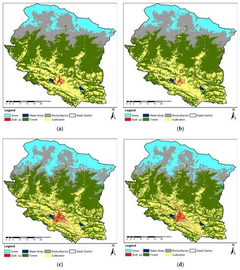
Figure 7.
LC Maps of Kaski district for two different time frames. (a) For 2010 using RF classifier; (b) for 2010 using XGBoost; (c) for 2020 using RF; (d) for 2020 using XGBoost.
Table 4.
Table showing overall accuracy, Kappa and no-information rate (NIR).
The validation data were divided proportionally according to the unsupervised classes, and hence the number of validation points was not the same for all the classes. Looking at the confusion matrix from Table A2 in Appendix A and producer accuracy in Table 5, we can understand that the PA of the built-up area in 2010 LC maps was 0. This is mainly because of having very few numbers of validation points for the built-up class, out of which one point of the validation set of the built-up class was misclassified as rocky/barren, and two points of the built-up class were misclassified as cultivation. The forest class was the most accurately classified class in both the years. The producer’s accuracy of forest in 2010 and 2020 were 0.93 and 0.98 for the RF classifier and 0.97 and 0.96 for the XGBoost classifier. We can see a significant difference in the performance of the classifier in water class. In 2010, the F1 score of water for the RF classifier was 0.67, whereas for XGBoost was 0.84. A similar trend can also be viewed for PA for 2010 and the F1 score and PA for 2020 for both classifiers. The main reason for the misclassification can be attributed to the same spectral signatures for two different classes in the Landsat image that led to the mismatch of pixels. Another constraint we experienced was with the shadow of hills and buildings that were misclassified as water. To mitigate this error, we took more distributed training data in those shadows and used multiple indices for classification. Other misclassification problems have occurred in the river’s sandy area as they were misclassified as the built-up area. These errors were mitigated by adopting a similar procedure, as discussed above. The error of misclassified pixels can be reduced by increasing the number of training dataset in that area. Though the increased number of training points minimizes the effect of the misclassified pixels, it may cause overfitting or high variance, i.e., high training accuracy but low testing accuracy during classification.
Table 5.
F1 score and producer accuracy for Landsat imagery used in the study.
After the implementation of accuracy assessment, the percentage change was measured, and the categorical compute change function was used from ArcGIS Pro to map the changes according to the category represented in Figure 8.
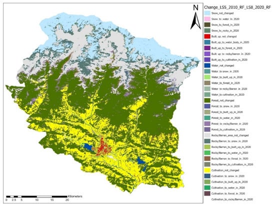
Figure 8.
LC change map for Kaski district from the year 2010 to the year 2020.
From the LC change map analysis, we can observe a major change in the main commercial area of the Kaski district, i.e., Pokhara. Pokhara’s LC has had tremendous change due to the development of recreational activities and improvements in the sightseeing area. The new international airport construction has converted about 1% of the total agricultural area to barren land. The built-up area has even shown an increasing trend. From the change map, we can also notice that the forest area has increased in the past decade. This may be due to the result of the increasing community forest plantation program. One other major change is from rocky to snow and vice versa. A major cause for this transition is the weather and climatic factors in this area. Rocky, barren land and cultivation areas have decreased from the previous year. The water area has not shown much change in terms of area, but the course of the river has changed in the past decade. The changes in area are shown in Figure 9.
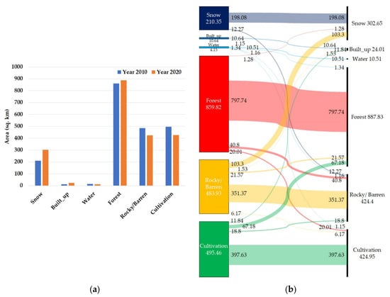
Figure 9.
Changes in the LC area from the year 2010 to the year 2020: (a) Bar diagram; (b) Sankey diagram.
The Sankey diagram from Figure 9 is the best graphical tool to represent the LC class change [68]. We can visualize how much area has changed from one category to every other category. We can see most of the land classes have not changed from 2010 to 2020. There was a huge change in rocky/ barren to snow in interclass change, i.e., approximately 104 sq km area was converted to snow. Another considerable transformation was the cultivation area. About 67.13 sq km of cultivation land was converted to forest in 2020. This implies a positive sign due to the increment of the community forest plantation program in the district in the last decade.
5. Discussion
We used a cloud-based computing platform (GEE) to acquire data (median composite, derivative indices and terrain) for Kaski District, Nepal and performed LC mapping using the ELMs in the CARET package of R. This has replaced the tedious and expensive process of map-making using traditional methods. This study presents an effective workflow of LC mapping and change detection using openly available tools. In this case study, we obtained good accuracy for all LC maps, resulting in a satisfactory outcome. For the RF classifier, the OA of 0.8792 +/− 0.0472 at the 95% confidence level was obtained for the 2010 LC map, whereas for 2020, the accuracy was 0.875 +/− 0.0575 at the 95% confidence level. For XGBoost, we obtained an accuracy of 0.8926 +/− 0.0448 at the 95% confidence level for the 2010 LC map, whereas for 2020, the accuracy was 0.8603 +/− 0.053 at the 95% confidence level. From this study, we can conclude that the Landsat imagery from EO data and GEE with ELMs are best for mapping the LC for a larger area. As RF performed better during the 2020 mapping and XGBoost model during the 2010 LC mapping, a clear distinction was not made on ELM’s performance.
LC mapping has been very limited in Nepal. The only national mapping organization of Nepal, the survey department (SD), still uses the traditional digitization technique for LC mapping for creating the national topographic database [10]. Although it is spatially more accurate, this process is labor-intensive and time-consuming. The process presented in this paper can be used for LC mapping with higher resolution satellite imagery to obtain a better result. The results of the LC mapping procedure were visually like that of the labor-intensive digitization mapping procedure of the SD. Both the model-simulated and observed LC map from SD are represented in Figure 10.
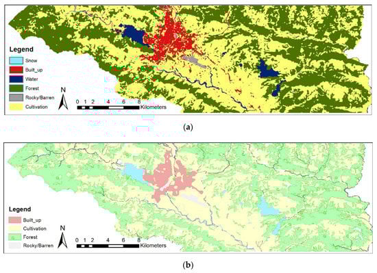
Figure 10.
LC map of Pokhara area of the year 2020: (a) Map obtained from our study procedure; (b) map from a topographical map from the survey department.
We also compared our LC map of the year 2010 with the LC map prepared by the International Centre for Integrated Mountain Development (ICIMOD). ICIMOD has produced a national LC map database of 2010 [69]. Although our map is not divided into broad categories as ICIMOD’s LC map, we can get a relatively similar result as ICIMOD’s LC map. Figure 11 shows the comparison of our LC map with ICIMOD’s LC map. By comparing both the maps, we can see the difference in the built-up area. This is because ICIMOD’s map is generalized, as it is performed for a larger area. With the exception of built-up, all classes showed similar characteristics when compared. Few works have been performed utilizing the ELMs. Abdi [42], in his study, used the RF and XGBoost classifiers to perform LC mapping using Sentinel 2 data. The author achieved an overall accuracy of 0.739 ± 0.018 for RF classifier and accuracy of 0.751 ± 0.017 for XGBoost. On the contrary, we obtained better accuracy by utilizing DEM data from SRTM using the GEE repository for mitigating the effects of hills and shadows and its misclassification. Another study by Talukdar et al. [40] implemented the RF classifier in the riparian landscape of the Ganges river and obtained an accuracy of 0.91. However, this study was conducted on a flat surface of India that has an elevation ranging from 15 m to 90 m, whereas our study was conducted in an area having elevation ranging from 300 m to 8091 m.
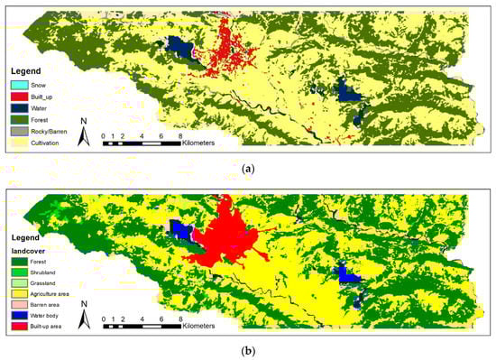
Figure 11.
LC map of Pokhara area of the year 2010: (a) Map obtained from our study procedure; (b) map prepared by ICIMOD.
From the beginning, there were various limitations and challenges to this work. The first challenge was related to the study area. As the Kaski district is heavily covered with clouds in the Landsat scene, it was challenging for us to get the perfect scene for mapping. The only possible solution was to consider the median composite of the annual Landsat imagery after cloud and snow masking. As we considered the median of the summer snow-covered and winter snow-covered images, the snow and rocky/barren areas were highly misclassified. Another limitation can be attributed to the presence of hills in the Kaski district. The shadows due to these hills caused the misclassification of forest and rocky areas as water bodies. Taking the reference data from those shadow areas and using the multiple indices helped us overcome this problem. The approaches presented in this study may be extended to generate a reliable, hierarchical, national-scale Nepal’s LC mapping. However, more challenges are expected when the study area is extended to the national scale (i.e., Nepal) with more cloud cover, fragmented landscapes and heterogeneous geography. The advances in technologies like cloud computing and AI has made it easier for automatic LC mapping.
Although sentinel imagery is available in the repository of the GEE, we have used Landsat imagery in our study because of the greater number of voids in the median composite of sentinel imagery even after cloud masking. Hence, we could not utilize and perform a proper study using sentinel imagery. While determining classes, we tried to incorporate all the LC classes as in Nepal Government’s topographic LC map, but due to higher mismatches in surface reflectivity, we were limited to only six classes. We tried to include grassland class on our map but failed due to a higher mismatch of pixels as the classifier trained in the Landsat imagery could not distinguish forest and grassland pixels.
In Nepal, huge snow and cloud covers make it impossible to map a large extent with the single-day image or even with the monthly composite image. Hence, the annual median composite adopted in this study can be adopted to make the LC map of entire Nepal which is openly available in the GEE platform. Such availability of data without extensive preprocessing and allocating substantial storage makes the process very fast and efficient. Future work can focus on implementing data fusion techniques for integrating Landsat and Sentinel imagery that may furnish greater accuracies with finer resolutions. Various other machine learning models with multitemporal resolutions (summer and winter composites) can be used for better understanding the models’ performance in LC mapping.
Author Contributions
Conceptualization, N.W. and T.D.A.; data curation, N.W. and T.D.A.; formal analysis, N.W. and T.D.A.; funding acquisition, D.H.L.; investigation, T.D.A., V.K. and H.H.; methodology, N.W. and T.D.A.; project administration, H.H. and D.H.L.; software, N.W.; supervision, H.H. and D.H.L.; validation, N.W.; visualization, T.D.A.; writing—original draft, N.W. and T.D.A.; writing—review and editing, V.K., H.H. and D.H.L. All authors have read and agreed to the published version of the manuscript.
Funding
This work was supported by the 2019 Research Grant (PoINT) funded by the Kangwon National University.
Conflicts of Interest
The authors declare no conflict of interest.
Appendix A

Figure A1.
Dot plot of the accuracy and Kappa in 95% confidence interval obtained by using various ntree for tuning random forest (RF) model: (a) for 2010 LC map (b) for 2020 LC map.

Figure A2.
Scatter plot of accuracy obtained by utilized all range of hyperparameter of XGBoost function tuning the model: (a) for 2010 LC map (b) for 2020 LC map.
Table A1.
Best hyperparameters for XGBoost classifier.
Table A1.
Best hyperparameters for XGBoost classifier.
| Year | 2010 | 2020 |
|---|---|---|
| nrounds | 200 | 200 |
| eta | 0.0025 | 0.1 |
| max_depth | 2 | 2 |
Table A2.
Confusion matrix generated in Google Earth Engine (GEE) for the validation dataset. Here 1 is built-up class, 2 is water class, 3 is forest class, 4 is rocky/barren class, and 5 is cultivation class.
Table A2.
Confusion matrix generated in Google Earth Engine (GEE) for the validation dataset. Here 1 is built-up class, 2 is water class, 3 is forest class, 4 is rocky/barren class, and 5 is cultivation class.
| Imagery | RF Classifier Reference | XGBoost Classifier Reference | |||||||||
|---|---|---|---|---|---|---|---|---|---|---|---|
| 1 | 2 | 3 | 4 | 5 | 1 | 2 | 3 | 4 | 5 | ||
| Landsat 5 (2010) Prediction | 1 | 0 | 0 | 0 | 0 | 1 | 0 | 0 | 0 | 1 | 0 |
| 2 | 0 | 7 | 0 | 1 | 3 | 0 | 8 | 0 | 1 | 0 | |
| 3 | 0 | 0 | 44 | 0 | 0 | 0 | 0 | 46 | 1 | 1 | |
| 4 | 1 | 2 | 2 | 35 | 0 | 1 | 1 | 1 | 32 | 1 | |
| 5 | 2 | 1 | 1 | 4 | 46 | 2 | 1 | 0 | 5 | 47 | |
| Landsat 8 (2020) Prediction | 1 | 4 | 0 | 0 | 1 | 3 | 5 | 0 | 0 | 2 | 3 |
| 2 | 2 | 8 | 0 | 4 | 0 | 1 | 8 | 0 | 3 | 0 | |
| 3 | 0 | 0 | 48 | 2 | 0 | 0 | 0 | 47 | 2 | 0 | |
| 4 | 1 | 0 | 1 | 36 | 0 | 1 | 0 | 2 | 35 | 1 | |
| 5 | 2 | 0 | 0 | 1 | 23 | 2 | 0 | 0 | 2 | 22 | |
References
- Bothara, J.; Ingham, J.; Dizhur, D. Earthquake risk reduction efforts in Nepal. In Integrating Disaster Science and Management; Elsevier: Amsterdam, The Netherlands, 2018; pp. 177–203. ISBN 9780128120569. [Google Scholar] [CrossRef]
- United Nations Department of Economic and Social Affairs Least Developed Country Category: Nepal Profile Department of Economic and Social Affairs. Available online: https://www.un.org/development/desa/dpad/least-developed-country-category-nepal.html (accessed on 10 October 2020).
- Subedi, S.; Bahadur Poudyal Chhetri, M. Impacts of the 2015 Gorkha Earthquake: Lessons Learnt from Nepal. Earthq. Impact Community Vulnerability Resil. 2019, 38. [Google Scholar] [CrossRef]
- Acharya, T.D.; Lee, D.H. Landslide Susceptibility Mapping using Relative Frequency and Predictor Rate along Araniko Highway. KSCE J. Civ. Eng. 2019, 23, 763–776. [Google Scholar] [CrossRef]
- Morell, K.D.; Sandiford, M.; Rajendran, C.P.; Rajendran, K.; Alimanovic, A.; Fink, D.; Sanwal, J. Geomorphology reveals active décollement geometry in the central Himalayan seismic gap. Lithosphere 2015, 7, 247–256. [Google Scholar] [CrossRef]
- Parajuli, J.; Haynes, K.E. Transportation network analysis in Nepal: A step toward critical infrastructure protection. J. Transp. Secur. 2018, 11, 101–116. [Google Scholar] [CrossRef]
- Venkatesh, K.; Ramesh, H. Impact of land use land cover change on run off generation in Tungabhadra river basin. ISPRS Ann. Photogramm. Remote Sens. Spat. Inf. Sci. 2018, 4, 367–374. [Google Scholar] [CrossRef]
- Subedi, A.; Poudel, P.; Acharya, T.D. Temporal shift of bagmati river over 25 years using landsat. In Proceedings of the International Archives of the Photogrammetry, Remote Sensing and Spatial Information Sciences—ISPRS Archives, Dhulikhel, Nepal, 10–11 December 2019; Volume 42, pp. 137–141. [Google Scholar]
- Venkatesh, K.; Ramesh, H.; Das, P. Modelling stream flow and soil erosion response considering varied land practices in a cascading river basin. J. Environ. Manag. 2020, 264, 110448. [Google Scholar] [CrossRef]
- Wagle, N.; Acharya, T.D. Past and present practices of topographic base map database update in Nepal. ISPRS Int. J. Geo-Inf. 2020, 9, 397. [Google Scholar] [CrossRef]
- Pang, R.; Huang, H.; Acharya, T.D. Spatiotemporal changes of riverbed and surrounding environment in Yongding river (Beijing section) in the past 40 years. J. Imaging Sci. Technol. 2020, 64. [Google Scholar] [CrossRef]
- Henderson-Sellers, A. (Ed.) Chapter 12 Human effects on climate through the large-scale impacts of land-use change. In World Survey of Climatology; Elsevier: Amsterdam, The Netherlands, 1995; Volume 16, pp. 433–475. ISBN 0168-6321. [Google Scholar]
- Acharya, T.D.; Lee, D.H. Remote Sensing and Geospatial Technologies for Sustainable Development: A Review of Applications. Sensors Mater. 2019, 31, 3931. [Google Scholar] [CrossRef]
- Pandey, P.C.; Koutsias, N.; Petropoulos, G.P.; Srivastava, P.K.; Ben Dor, E. Land use/land cover in view of earth observation: Data sources, input dimensions, and classifiers—A review of the state of the art. Geocarto Int. 2019, 1–32. [Google Scholar] [CrossRef]
- Acharya, T.D.; Yang, I.T.; Lee, D.H. Land Cover Classification of Imagery from Landsat Operational Land Imager Based on Optimum Index Factor. Sensors Mater. 2018, 30, 1753. [Google Scholar] [CrossRef]
- Mayaux, P.; Eva, H.; Brink, A.; Achard, F.; Belward, A. Remote Sensing of Land-Cover and Land-Use Dynamics. In Earth Observation of Global Change: The Role of Satellite Remote Sensing in Monitoring the Global Environment; Springer: Dordrecht, The Netherlands, 2008; pp. 85–108. ISBN 9781402063572. [Google Scholar]
- Wulder, M.A.; White, J.C.; Goward, S.N.; Masek, J.G.; Irons, J.R.; Herold, M.; Cohen, W.B.; Loveland, T.R.; Woodcock, C.E. Landsat continuity: Issues and opportunities for land cover monitoring. Remote Sens. Environ. 2008, 112, 955–969. [Google Scholar] [CrossRef]
- Alam, A.; Bhat, M.S.; Maheen, M. Using Landsat satellite data for assessing the land use and land cover change in Kashmir valley. GeoJournal 2019, 0123456789. [Google Scholar] [CrossRef]
- Hansen, M.C.; Loveland, T.R. A review of large area monitoring of land cover change using Landsat data. Remote Sens. Environ. 2012, 122, 66–74. [Google Scholar] [CrossRef]
- Berhane, T.M.; Lane, C.R.; Mengistu, S.G.; Christensen, J.; Golden, H.E.; Qiu, S.; Zhu, Z.; Wu, Q. Land-cover changes to surface-water buffers in the midwestern USA: 25 years of landsat data analyses (1993–2017). Remote Sens. 2020, 12, 754. [Google Scholar] [CrossRef]
- Potapov, P.; Hansen, M.C.; Kommareddy, I.; Kommareddy, A.; Turubanova, S.; Pickens, A.; Adusei, B.; Tyukavina, A.; Ying, Q. Landsat analysis ready data for global land cover and land cover change mapping. Remote Sens. 2020, 12, 426. [Google Scholar] [CrossRef]
- Lin, Y.; Zhang, L.; Wang, N.; Zhang, X.; Cen, Y.; Sun, X. A change detection method using spatial-temporal-spectral information from Landsat images. Int. J. Remote Sens. 2020, 41, 772–793. [Google Scholar] [CrossRef]
- Rathnayake, W.M.C.; Jones, S.; Soto-Berelov, M. Mapping land cover change over a 25-year period (1993–2018) in Sri Lanka using landsat time-series. Land 2020, 9, 27. [Google Scholar] [CrossRef]
- Shi, X.; Deng, Z.; Ding, X.; Li, L. Land cover classification combining Sentinel-1 and Landsat 8 imagery driven by Markov random field with amendment reliability factors. Eurasip J. Wirel. Commun. Netw. 2020, 2020. [Google Scholar] [CrossRef]
- Damtea, W.; Kim, D.; Im, S. Spatiotemporal analysis of land cover changes in the chemoga basin, Ethiopia, using Landsat and google earth images. Sustainability 2020, 12, 3607. [Google Scholar] [CrossRef]
- Senf, C.; Laštovička, J.; Okujeni, A.; Heurich, M.; van der Linden, S. A generalized regression-based unmixing model for mapping forest cover fractions throughout three decades of Landsat data. Remote Sens. Environ. 2020, 240. [Google Scholar] [CrossRef]
- Ha, T.V.; Tuohy, M.; Irwin, M.; Tuan, P.V. Monitoring and mapping rural urbanization and land use changes using Landsat data in the northeast subtropical region of Vietnam. Egypt. J. Remote Sens. Sp. Sci. 2020, 23, 11–19. [Google Scholar] [CrossRef]
- Acharya, T.D.; Subedi, A.; Lee, D.H. Evaluation of machine learning algorithms for surface water extraction in a landsat 8 scene of nepal. Sensors (Switzerland) 2019, 19, 2769. [Google Scholar] [CrossRef] [PubMed]
- Acharya, T.D.; Subedi, A.; Lee, D.H. Evaluation of water indices for surface water extraction in a landsat 8 scene of Nepal. Sensors (Switzerland) 2018, 18, 2580. [Google Scholar] [CrossRef] [PubMed]
- Kulkarni, A.D.; Lowe, B. Random Forest Algorithm for Land Cover Classification. Int. J. Recent Innov. Trends Comput. Commun. 2016, 4, 58–63. [Google Scholar]
- Acharya, T.D.; Yang, I.T.; Lee, D.H. Land cover classification using a KOMPSAT-3A multi-spectral satellite image. Appl. Sci. 2016, 6, 371. [Google Scholar] [CrossRef]
- Brodley, C.E.; Friedl, M.A. Decision tree classification of land cover from remotely sensed data. Remote Sens. Environ. 1997, 61, 399–409. [Google Scholar] [CrossRef]
- Nomura, K.; Mitchard, E.T.A. More than meets the eye: Using Sentinel-2 to map small plantations in complex forest landscapes. Remote Sens. 2018, 10, 1693. [Google Scholar] [CrossRef]
- Xie, S.; Liu, L.; Zhang, X.; Yang, J.; Chen, X.; Gao, Y. Automatic land-cover mapping using landsat time-series data based on google earth engine. Remote Sens. 2019, 11, 3023. [Google Scholar] [CrossRef]
- Sidhu, N.; Pebesma, E.; Câmara, G. Using Google Earth Engine to detect land cover change: Singapore as a use case. Eur. J. Remote Sens. 2018, 51, 486–500. [Google Scholar] [CrossRef]
- Noi Phan, T.; Kuch, V.; Lehnert, L.W. Land cover classification using google earth engine and random forest classifier-the role of image composition. Remote Sens. 2020, 12, 2411. [Google Scholar] [CrossRef]
- Oliphant, A.J.; Thenkabail, P.S.; Teluguntla, P.; Xiong, J.; Gumma, M.K.; Congalton, R.G.; Yadav, K. Mapping cropland extent of Southeast and Northeast Asia using multi-year time-series Landsat 30-m data using a random forest classifier on the Google Earth Engine Cloud. Int. J. Appl. Earth Obs. Geoinf. 2019, 81, 110–124. [Google Scholar] [CrossRef]
- Phalke, A.R.; Özdoğan, M.; Thenkabail, P.S.; Erickson, T.; Gorelick, N.; Yadav, K.; Congalton, R.G. Mapping croplands of Europe, Middle East, Russia, and Central Asia using Landsat, Random Forest, and Google Earth Engine. ISPRS J. Photogramm. Remote Sens. 2020, 167, 104–122. [Google Scholar] [CrossRef]
- Li, Q.; Qiu, C.; Ma, L.; Schmitt, M.; Zhu, X.X. Mapping the land cover of africa at 10 m resolution from multi-source remote sensing data with google earth engine. Remote Sens. 2020, 12, 602. [Google Scholar] [CrossRef]
- Zeng, H.; Wu, B.; Wang, S.; Musakwa, W.; Tian, F.; Mashimbye, Z.E.; Poona, N.; Syndey, M. A Synthesizing Land-cover Classification Method Based on Google Earth Engine: A Case Study in Nzhelele and Levhuvu Catchments, South Africa. Chin. Geogr. Sci. 2020, 30, 397–409. [Google Scholar] [CrossRef]
- Shelestov, A.; Lavreniuk, M.; Kussul, N.; Novikov, A.; Skakun, S. Exploring Google earth engine platform for big data processing: Classification of multi-temporal satellite imagery for crop mapping. Front. Earth Sci. 2017, 5, 1–10. [Google Scholar] [CrossRef]
- Abdi, A.M. Land cover and land use classification performance of machine learning algorithms in a boreal landscape using Sentinel-2 data. GIScience Remote Sens. 2020, 57, 1–20. [Google Scholar] [CrossRef]
- Jamali, A. Land use land cover modeling using optimized machine learning classifiers: A case study of Shiraz, Iran. Model. Earth Syst. Environ. 2020. [Google Scholar] [CrossRef]
- Talukdar, S.; Singha, P.; Mahato, S.; Shahfahad; Pal, S.; Liou, Y.A.; Rahman, A. Land-use land-cover classification by machine learning classifiers for satellite observations-A review. Remote Sens. 2020, 12, 1135. [Google Scholar] [CrossRef]
- Breiman, L. Arcing classifiers. Ann. Stat. 1998, 26. [Google Scholar] [CrossRef]
- Breiman, L. Bagging predictors. Mach. Learn. 1996, 24. [Google Scholar] [CrossRef]
- Nurfadila, J.S.; Baja, S.; Neswati, R.; Rukmana, D.; Zylshal, Z. Initial Results on Landuse/Landcover Classification Using Pixel-Based Random Forest Algorithm on Sentinel-2 Imagery over Enrekang Region. In Proceedings of the IOP Conference Series: Earth and Environmental Science, Kyoto, Japan, 17–21 September 2019; Volume 280. [Google Scholar]
- Georganos, S.; Grippa, T.; Vanhuysse, S.; Lennert, M.; Shimoni, M.; Wolff, E. Very High Resolution Object-Based Land Use-Land Cover Urban Classification Using Extreme Gradient Boosting. IEEE Geosci. Remote Sens. Lett. 2018, 15, 607–611. [Google Scholar] [CrossRef]
- Isaac, E.; Easwarakumar, K.S.; Isaac, J. Urban landcover classification from multispectral image data using optimized AdaBoosted random forests. Remote Sens. Lett. 2017, 8. [Google Scholar] [CrossRef]
- GENESIS Consultancy Pvt. Ltd. Report on Impact of Settlement Pattern, Land–Use Practice and Options in High Risk Areas, Pokhara Sub-Metropolitan City; Report for UNDP/ERRRP UNDP/ERRRP’s Earthquake Risk Reduction and Recovery Preparedness Program for Nepal; GENESIS Consultancy Pvt. Ltd.: Lalitpur, Nepal, 2009. [Google Scholar]
- U.S. Geological Survey. Landsat 8 Data Users Handbook; U.S. Geological Survey: Reston, VA, USA, 2016; Volume 8. [Google Scholar]
- USGS Landsat Mission- Landsat 5. Available online: https://www.usgs.gov/core-science-systems/nli/landsat/landsat-5?qt-science_support_page_related_con=0#qt-science_support_page_related_con (accessed on 10 October 2020).
- Landsat 4-7 Surface Reflectance Quality Assessment. Available online: https://www.usgs.gov/core-science-systems/nli/landsat/landsat-4-7-surface-reflectance-quality-assessment?qt-science_support_page_related_con=1#qt-science_support_page_related_con (accessed on 10 October 2020).
- USGS Landsat Surface Reflectance Quality Assessment. Available online: https://landsat.usgs.gov/landsat-surface-reflectance-quality-assessment (accessed on 10 October 2020).
- USGS CFMask Algorithm. Available online: https://www.usgs.gov/land-resources/nli/landsat/cfmask-algorithm (accessed on 10 October 2020).
- Hennig, T.A.; Kretsch, J.L.; Pessagno, C.J.; Salamonowicz, P.H.; Stein, W.L. The shuttle radar topography mission. Lect. Notes Comput. Sci. (Incl. Subser. Lect. Notes Artif. Intell. Lect. Notes Bioinform.) 2001, 2181, 65–77. [Google Scholar] [CrossRef]
- Farr, T.G.; Rosen, P.A.; Caro, E.; Crippen, R.; Duren, R.; Hensley, S.; Kobrick, M.; Paller, M.; Rodriguez, E.; Roth, L.; et al. The shuttle radar topography mission. Rev. Geophys. 2007, 45. [Google Scholar] [CrossRef]
- Measuring Vegetation (NDVI & EVI). Available online: https://earthobservatory.nasa.gov/features/MeasuringVegetation/measuring_vegetation_2.php (accessed on 10 October 2020).
- Macarof, P.; Statescu, F. Comparasion of NDBI and NDVI as Indicators of Surface Urban Heat Island Effect in Landsat 8 Imagery: A Case Study of Iasi. Present Environ. Sustain. Dev. 2017, 11, 141–150. [Google Scholar] [CrossRef]
- Krishna, H. Study of normalized difference built-up (NDBI) index in automatically mapping urban areas from Landsat TM imagery. Int. J. Eng. Sci. 2018, 7, 1–8. [Google Scholar]
- Feyisa, G.L.; Meilby, H.; Fensholt, R.; Proud, S.R. Automated Water Extraction Index: A new technique for surface water mapping using Landsat imagery. Remote Sens. Environ. 2014, 140, 23–35. [Google Scholar] [CrossRef]
- Breiman, L. Random forests. Mach. Learn. 2001, 45, 5–32. [Google Scholar] [CrossRef]
- Chen, T.; Guestrin, C. XGBoost: A scalable tree boosting system. In Proceedings of the 22nd ACM Sigkdd International Conference on Knowledge Discovery and Data Mining, 13–17 August 2016; pp. 785–794. [Google Scholar] [CrossRef]
- Rwanga, S.S.; Ndambuki, J.M. Accuracy Assessment of Land Use/Land Cover Classification Using Remote Sensing and GIS. Int. J. Geosci. 2017, 8, 611–622. [Google Scholar] [CrossRef]
- Cohen, J. A Coefficient of Agreement for Nominal Scales. Educ. Psychol. Meas. 1960, 20, 37–46. [Google Scholar] [CrossRef]
- Sasaki, Y. The truth of the F-measure The truth of the F-measure. Teach Tutor Mater 2015, 1–6. Available online: https://www.cs.odu.edu/~mukka/cs795sum09dm/Lecturenotes/Day3/F-measure-YS-26Oct07.pdf (accessed on 10 October 2020).
- Powers, D. Ailab Evaluation: From precision, recall and F-measure to ROC, informedness, markedness & correlation. J. Mach. Learn. Technol 2011, 2, 2229–3981. [Google Scholar] [CrossRef]
- Cuba, N. Research note: Sankey diagrams for visualizing land cover dynamics. Landsc. Urban Plan. 2015, 139, 163–167. [Google Scholar] [CrossRef]
- Uddin, K.; Shrestha, H.L.; Murthy, M.S.R.; Bajracharya, B.; Shrestha, B.; Gilani, H.; Pradhan, S.; Dangol, B. Development of 2010 national land cover database for the Nepal. J. Environ. Manag. 2015, 148, 82–90. [Google Scholar] [CrossRef] [PubMed]
Publisher’s Note: MDPI stays neutral with regard to jurisdictional claims in published maps and institutional affiliations. |
© 2020 by the authors. Licensee MDPI, Basel, Switzerland. This article is an open access article distributed under the terms and conditions of the Creative Commons Attribution (CC BY) license (http://creativecommons.org/licenses/by/4.0/).