Article

Analytical Solutions of (2+Time Fractional Order) Dimensional Physical Models, Using Modified Decomposition Method

1
Department of Mathematics, Abdul Wali khan University, Mardan 23200, Pakistan
2
Department of Mathematics, Faculty of Arts and Sciences, Cankaya University, 06530 Ankara, Turkey
3
Institute of Space Sciences, 077125 Magurele-Bucharest, Romania
4
Center of Excellence in Theoretical and Computational Science (TaCS-CoE) & Department of Mathematics, Faculty of Science, King Mongkut’s University of Technology Thonburi (KMUTT), 126 Pracha Uthit Rd., Bang Mod, Thung Khru, Bangkok 10140, Thailand
5
Department of Medical Research, China Medical University Hospital, China Medical University, Taichung 40402, Taiwan
*
Author to whom correspondence should be addressed.
Appl. Sci. 2020, 10(1), 122; https://doi.org/10.3390/app10010122
Submission received: 24 October 2019 / Revised: 13 November 2019 / Accepted: 21 November 2019 / Published: 23 December 2019

Abstract

:
In this article, a new analytical technique based on an innovative transformation is used to solve (2+time fractional-order) dimensional physical models. The proposed method is the hybrid methodology of Shehu transformation along with Adomian decomposition method. The series form solution is obtained by using the suggested method which provides the desired rate of convergence. Some numerical examples are solved by using the proposed method. The solutions of the targeted problems are represented by graphs which have confirmed closed contact between the exact and obtained solutions of the problems. Based on the novelty and straightforward implementation of the method, it is considered to be one of the best analytical techniques to solve linear and non-linear fractional partial differential equations.

1. Introduction

Fractional calculus is considered to be a powerful tool for modeling complex phenomenon. Recently, the researchers have shown the greatest interest towards fractional calculus because of its numerous applications in different fields of sciences. Despite complicated background of fractional calculus, it came into being from simple question of L’Hospital. The first order represent slope of a function, what will it represent for fractional order ( 1 2 ) ? To find the answer of this question, the mathematicians have managed to open a new window of opportunities to improve the mathematical modeling of real world problems, which has given birth to many new questions and intriguing results. These newly established results have numerous implementation in many areas of engineering [1,2], such as fractional-order Buck master and diffusion problems [3], fractional-order telegraph model [4,5], fractional KdV-Burger-Kuramoto equation [6], fractal vehicular traffic flow [7], fractional Drinfeld-Sokolov-Wilson equation [8], fractional-order anomalous sub-diffusion model [9], fractional design of hepatitis B virus [10], fractional modeling chickenpox disease [11], fractional blood ethanol concentration model [12], fractional model for tuberculosis [13], fractional vibration equation [14], fractional Black-Scholes option pricing equations [15], fractionally damped beams [16], fractionally damped coupled system [17], fractional-order heat, wave and diffusion equations [18,19], fractional order pine wilt disease model [20], fractional diabetes model [21] etc.
Nowadays, the focus of the researchers is to develop different numerical and analytical techniques for the solution of fractional-order models. Therefore, different types of analytical and numerical methods have been developed and used for the solution of different fractional models. The analytical algorithm, the history of integral transform traced back to the time when Laplace started work an integral transform in 1780 s and Joseph Fourier in 1822. Integral transformations are without question one of the most useful and effective methods in theoretical and applied mathematics, with numerous uses in quantum physics, mechanical engineering and several other areas of science. Moreover, the integral transform is used in chemistry, architecture, and other social sciences to evaluate various models [22]. In recent years, different integral transform such as Laplace transform [23,24,25] , Fourier transform [26,27], Hankel transform [28], Mellin transform [29], Z-transform [30], Wavelet transform [31], Elzaki transform [32,33], Mahgoub transform [34], Aboodh transform [35], Mohand transform [36], Sumudu transform [37,38], Hermite transform [39] etc have been used for the solution of different physical models.
Originality of the paper: In this article, we have applied a new analytical technique, which is based on generalization of sumudu and laplace transform with Adomian decomposition method (ADM) to solve (2+time fractional-order) dimensional physical models. In the present research we have analyzed the fractional view of some important physical problems by using Shehu decomposition method (SDM). Some important fractional-order problems are solved, which provide the best information about the targeted physical problems as compare to integer-order problems solution. The results of the integer-order problem are compared with the fractional-order problems. In conclusion, in the present research work, we provided and improved the existing physical models of integer-order by using the idea of fractional calculus. The modified mathematical models of fractional-order derivative are solved by using a new and sophisticated analytical method. Moreover, the proposed analytical method has provided the solutions of the problems that have a very close contact with the exact solutions of the problems. The methodology can be extended towards other fractional-order partial differential equations, that are frequently occurred in science and engineering.
The rest of the paper is organized as: In Section 2, we presented the basic definitions and theorem of the proposed method. In Section 3, we have discussed the implementation of proposed transformation. In Section 4 we evaluated the numerical examples by using the proposed technique and discussed the plots. In Section 5 we lastly summarized our results.

2. Preliminaries Concepts

In this section, we present some fundamental and appropriate definitions and preliminary concepts related to the fractional calculus and the Shehu transformation.
Definition 1.
Shehu transform
Shehu transformation is new and similar to other integral transformation which is defined for functions of exponential order [40]. We take a function in the set A define by
A = { u ( τ ) : , ρ 1 , ρ 2 > 0 , | u ( τ ) | < M e | τ | ρ i , i f τ [ 0 , ) ,
The Shehu transform which is represented by S ( . ) for a function u ( τ ) is defined as
S { u ( τ ) } = V ( s , μ ) = 0 u ( τ ) e s τ μ u ( τ ) d τ , τ > 0 , s > 0 .
The Shehu transform of a function u ( τ ) is V ( s , μ ) : then u ( τ ) is called the inverse of V ( s , μ ) which is expressed as
S 1 V ( s , μ ) = u ( τ ) , f o r τ 0 , S 1 i s i n v e r s e S h e h u t r a n s f o r m .
Definition 2.
Shehu transform for nth derivatives
The Shehu transformation for nth derivatives is defined as [40]
S u ( n ) ( τ ) = s n μ n V ( s , μ ) k = 0 n 1 s μ n k 1 u ( k ) ( 0 ) .
Definition 3.
Caputo operator of fractional partial derivative
The fractional Caputo operator is represented as [41]
D τ β f ( τ ) = n f ( τ ) τ n , β = n N , 1 Γ ( n β ) 0 τ ( τ ϕ ) n β 1 f ( n ) ( ϕ ) ϕ , n 1 < β n , n N .
Definition 4.
Shehu transform for fractional order derivatives
The Shehu transformation for the fractional order derivatives is expressed as
S u ( β ) ( τ ) = s β μ β V ( s , μ ) k = 0 n 1 s μ β k 1 u ( k ) ( 0 ) , 0 < β n ,
In Table 1 show different special functions of Shehu transformation.
Theorem 1.
If the function u ( τ ) is piecewise continues at every finite interval of 0 τ β and of exponential order α for τ > β , then there’s the Shehu transform u ( s , μ ) [40].
Proof. 
For any natural number β , we deduct algebraically:
0 e x p ( s τ μ ) u ( τ ) d τ = 0 β e x p ( s τ μ ) u ( τ ) d τ + β e x p ( s τ μ ) u ( τ ) d τ ,
since the function u ( τ ) continues in a piecewise manner at every finite interval 0 τ β , there’s the first integral on the right hand side. We suggest the following situation to validate this statement,
| α e x p ( s τ μ ) u ( τ ) d τ | α | e x p ( s τ μ ) u ( τ ) | d τ α e x p ( s τ μ ) | u ( τ ) | d τ α e x p ( s τ μ ) N e x p ( β τ ) d τ = N α e x p ( ( s β u ) τ u ) d τ = N u ( s β u ) lim γ e x p ( ( s β u ) τ u ) d τ 0 γ = N u ( s β u ) .
The proof is complete. □

3. Implementation of Shehu Transform

In this section, we have considered a time fractional (2+time fractional-order) dimensional physical model in the form
u τ β ( , , τ ) = κ u ( , , τ ) + £ u ( , , τ ) + u ( , , τ ) , β [ 1 , 2 ]
with initial condition
u ( , , 0 ) = u ( , ) ,
while κ is a non-linear operator and £ linear operator.
Applying the Shehu transform to both sides of the Equation (9) we obtain
S u τ β ( , , τ ) = S κ u ( , , τ ) + £ u ( , , τ ) + u ( , , τ ) , β [ 1 , 2 ] .
Using the differential property of Shehu transformation we have,
s β μ β V ( s , μ ) μ s u ( 0 ) μ 2 s 2 u ( 0 ) = S κ u ( , , τ ) + £ u ( , , τ ) + u ( , , τ ) .
Simplifying Equation (12), we obtain
V ( s , μ ) = + μ β s β S κ u ( , , τ ) + £ u ( , , τ ) + u ( , , τ ) + μ s u ( 0 ) + μ 2 s 2 u ( 0 ) .
Applying the inverse Shehu transformation, we get
u ( , , τ ) = S 1 μ β s β S κ u ( , , τ ) + £ u ( , , τ ) + u ( , , τ ) + u ( 0 ) + τ u ( 0 ) .
The nonlinear term u ( , , τ ) is evaluated by using the procedure of Adomian polynomial decomposition given by
u ( , , τ ) = m = 0 A m ( u 0 , u 1 , ) , m = 0 , 1 ,
where,
A m ( u 0 , u 1 , ) = 1 m ! d m d λ m i = 0 λ i u i λ = 0 , m > 0 .
With the help of Equation (16), Equation (15) can be written as
u ( , , τ ) = S 1 μ β s β S κ u ( , , τ ) + £ u ( , , τ ) + m = 0 A m + u ( 0 ) + τ u ( 0 ) .
Finally, we obtain the recursive relation as
u 0 ( , , τ ) = u ( 0 ) + τ u ( 0 ) , m = 0 u m ( , , τ ) = S 1 μ β s β S κ u ( m 1 ) ( , , τ ) + £ u ( m 1 ) ( , , τ ) + u ( m 1 ) ( , , τ ) + m = 0 A m , m 1 .

4. Applications and Discussion

Example 1.
Consider the (2+time fractional-order) dimensional hyperbolic wave model:
u τ β ( , , τ ) = 1 12 2 u ( , , τ ) + 1 12 2 u ( , , τ ) , β ( 1 , 2 )
with initial conditions
u ( , , 0 ) = 4 , u τ ( , , 0 ) = 4 .
If β = 2 , then the exact solution of Equation (19) is
u ( , , τ ) = 4 sinh ( t ) + 4 cosh ( t ) ,
Taking the Shehu transform of Equation (19) we obtain
s β μ β V ( s , μ ) μ s u ( 0 ) μ 2 s 2 u ( 0 ) = S 1 12 2 u ( , , τ ) + 1 12 2 u ( , , τ ) .
Simplifying Equation (22), we get
V ( s , μ ) = μ β s β S 1 12 2 u ( , , τ ) + 1 12 2 u ( , , τ ) + μ s u ( 0 ) + μ 2 s 2 u ( 0 ) .
Applying inverse Shehu transform, we get
u ( , , τ ) = u ( 0 ) + u ( 0 ) τ + S 1 μ β s β S 1 12 2 u ( , , τ ) + 1 12 2 u ( , , τ ) .
Thus we get the following recursive scheme
u 0 ( , , τ ) = u ( 0 ) + u ( 0 ) τ = 4 + 4 τ ,
u m + 1 ( , , τ ) = S 1 μ β s β S 1 12 2 u m ( , , τ ) + 1 12 2 u m ( , , τ ) .
Using Equation (26), for m = 0 , 1 , 2 , 3 , we get the following values
u 1 ( , , τ ) = 4 τ β β ! + 4 τ β + 1 ( β + 1 ) ! , u 2 ( , , τ ) = 4 τ 2 β ( 2 β ) ! + 4 τ 2 β + 1 ( 2 β + 1 ) ! , u 3 ( , , τ ) = 4 τ 3 β ( 3 β ) ! + 4 τ 3 β + 1 ( 3 β + 1 ) ! , u 4 ( , , τ ) = 4 τ 4 β ( 4 β ) ! + 4 τ 4 β + 1 ( 4 β + 1 ) ! ,
Now using the values of u 0 , u 1 , u 2 , u 3 , , we get Shehu transformation solution for example 1
u ( , , τ ) = 4 + 4 τ + 4 τ β β ! + 4 τ β + 1 ( β + 1 ) ! + 4 τ 2 β ( 2 β ) ! + 4 τ 2 β + 1 ( 2 β + 1 ) ! + 4 τ 3 β ( 3 β ) ! + 4 t 3 β + 1 ( 3 β + 1 ) ! + 4 τ 4 β ( 4 β ) ! + 4 τ 4 β + 1 ( 4 β + 1 ) ! +
After simplification, we get
u ( , , τ ) = 4 1 + τ β β ! + τ 2 β ( 2 β ) ! + τ 3 β ( 3 β ) ! + τ 4 β ( 4 β ) ! + + 4 τ + τ β + 1 ( β + 1 ) ! + τ 2 β + 1 ( 2 β + 1 ) ! + τ 3 β + 1 ( 3 β + 1 ) ! + τ 4 β + 1 ( 4 β + 1 ) ! + .
In particular, when β 2 , the analytical solution of Shehu transform become as
u ( , , τ ) = 4 1 + τ 2 2 ! + τ 4 ( 4 ) ! + τ 6 ( 6 ) ! + τ 8 ( 8 ) ! + + 4 τ + τ 3 ( 3 ) ! + τ 5 ( 5 ) ! + τ 7 ( 7 ) ! + τ 9 ( 9 ) ! + ,
which provide the close form solution as
u ( , , τ ) = 4 cosh ( τ ) + 4 sinh ( τ ) .
Figure 1 and Figure 2 represent the exact and analytical solutions of Example 1. The solutions-graphs have confirmed the closed contact between the exact solution and the analytical solution obtained by the proposed method. In Figure 3, the solution of Example 1 are calculated at different fractional-order β of the derivative. It is investigated that the solutions at different fractional-orders β are convergent to an integer-order solution of Example 1. Figure 4 represent the solution verses time graph for Example 1. It is observed that as the time fractional-order varies toward time integer-order, the time fractional-order solutions also approaches to the solution of an integer-order problem of Example 1. All the above solution analysis of Example 1 indicate that SDM is an efficient and effective method to solve fractional-order partial differential equations that are frequently arising in science and engineering.
In Table 2, the solutions of Shehu transform decomposition method (SDM) and Adomian decomposition method (ADM) are compared with each other. The comparison has shown that the solutions of proposed method are in strong agreement with the solution of ADM.
Example 2.
Consider the (2+time fractional-order) dimensional Heat model:
u τ β ( , , τ ) = u ( , , τ ) + u ( , , τ ) , β ( 0 , 1 ]
with initial condition
u ( , , 0 ) = sin ( ) cos ( ) .
If β = 1 , then the exact solution of Equation (32) is
u ( , , τ ) = e 2 τ sin ( ) cos ( ) .
Taking Shehu transform of Equation (32)
s β μ β V ( s , μ ) μ s u ( 0 ) = S u ( , , τ ) + u ( , , τ ) ,
Simplifying Equation (35), we get as
V ( s , μ ) = μ s u ( 0 ) + μ β s β S u ( , , τ ) + u ( , , τ ) .
Applying inverse Shehu transform, we get
u ( , , τ ) = u ( 0 ) + S 1 μ β s β S u ( , , τ ) + u ( , , τ ) .
Thus we get the following recursive scheme
u 0 ( , , τ ) = u ( 0 ) = sin ( ) cos ( ) ,
u m + 1 ( , , τ ) = S 1 μ β s β S u m ( , , τ ) + u m ( , , τ ) ,
Using Equation (39), for m = 0 , 1 , 2 , 3 , we get the following values
u 1 ( , , τ ) = 2 sin ( ) cos ( ) τ β ( β ) ! , u 2 ( , , τ ) = 4 sin ( ) cos ( ) τ 2 β ( 2 β ) ! , u 3 ( , , τ ) = 8 sin ( ) cos ( ) τ 3 β ( 3 β ) ! , u 4 ( , , τ ) = 16 sin ( ) cos ( ) τ 4 β ( 4 β ) ! ,
Now using the values of u 0 , u 1 , u 2 , u 3 , , we get Shehu transformation solution for example 2
u ( , , τ ) = sin ( ) cos ( ) 2 sin ( ) cos ( ) τ β ( β ) ! + 4 sin ( ) cos ( ) τ 2 β ( 2 β ) ! + 8 sin ( ) cos ( ) τ 3 β ( 3 β ) ! + 16 sin ( ) cos ( ) τ 4 β ( 4 β ) ! +
After simplification, we get
u ( , , τ ) = sin ( ) cos ( ) 1 2 τ β ( β ) ! + 4 τ 2 β ( 2 β ) ! + 8 τ 3 β ( 3 β ) ! + 16 τ 4 β ( 4 β ) ! + ,
which converge to the solution
u ( , , τ ) = sin ( ) cos ( ) E β ( 2 τ β ) ,
For particular case β 1 , the Shehu transform solution become as
u ( , , τ ) = sin ( ) cos ( ) e 2 τ .
Figure 5 and Figure 6 show the exact and analytical solution of Example 2 respectively. The graphical representation have confirmed the closed contact of the obtained solution with the exact solution of Example 2. Similarly, Figure 7 and Figure 8 represents the fractional-order solution of Example 2 for two and three space. Both graphs support the convergence phenomena of fractional-order problems to an integer-order problem of Example 2.
Example 3.
Consider the ( 2 + t i m e f r a c t i o n a l ) dimensional diffusion model:
u τ β ( , , τ ) = u ( , , τ ) + u ( , , τ ) , β ( 0 , 1 ]
with the initial condition
u ( , , 0 ) = e + .
If β = 1 , then the exact solution of Equation (45) is
u ( , , τ ) = e + + 2 τ
Taking Shehu transform of Equation (45)
s β μ β V ( s , μ ) μ s u ( 0 ) = S u ( , , τ ) + u ( , , τ ) .
Simplifying Equation (46), we get as
V ( s , μ ) = μ s u ( 0 ) + μ β s β S u ( , , τ ) + u ( , , τ ) .
Applying inverse operator of Shehu transform, we get
u ( , , τ ) = u ( 0 ) + S 1 μ β s β S u ( , , τ ) + u ( , , τ ) .
Thus we get the following recursive scheme
u 0 ( , , τ ) = u ( 0 ) = e + ,
u m + 1 ( , , τ ) = S 1 μ β s β S u m ( , , τ ) + u m ( , , τ ) ,
Using Equation (51), for m = 0 , 1 , 2 , 3 , we get the following values
u 1 ( , , τ ) = 2 e + τ β ( β ) ! , u 2 ( , , τ ) = 4 e + τ 2 β ( 2 β ) ! , u 3 ( , , τ ) = 8 e + τ 3 β ( 3 β ) ! , u 4 ( , , τ ) = 16 e + τ 4 β ( 4 β ) ! ,
Now using the values of u 0 , u 1 , u 2 , u 3 , , we get Shehu transformation solution for Example 3
u ( , , τ ) = e + + 2 e + τ β ( β ) ! + 4 e + τ 2 β ( 2 β ) ! + 8 e + τ 3 β ( 3 β ) ! + 16 e + τ 4 β ( 4 β ) ! + .
After simplification, we get
u ( , , τ ) = sin ( ) cos ( ) 1 + 2 τ β ( β ) ! + 4 τ 2 β ( 2 β ) ! + 8 τ 3 β ( 3 β ) ! + 16 τ 4 β ( 4 β ) ! + .
The close form solution become as
u ( , , τ ) = sin ( ) cos ( ) E β ( 2 τ β ) .
When β 1 the calculated result provide the exact solution in the close form
u ( , , τ ) = sin ( ) cos ( ) e 2 τ .
Figure 9 and Figure 10 show the exact and analytical solutions of Example 3. Both figures are almost coincident confirming the close contact of both exact and obtained solution. Figure 11 the SDM solutions at different fractional-order β are calculated for Example 3. The convergence phenomena of fractional-order solution towards exact solution is observed. The method is found to be very simple and straightforward to solve fractional-order different equations.
Example 4.
Consider the ( 2 + t i m e f r a c t i o n a l ) dimensional telegraph model:
u τ β ( , , τ ) = 1 2 u ( , , τ ) + 1 2 u ( , , τ ) 2 u t ( , , τ ) u ( , , τ ) , β ( 1 , 2 ] ,
with initial conditions
u ( , , 0 ) = sinh ( ) sinh ( ) , u τ ( , , 0 ) = 2 sinh ( ) sinh ( ) .
If β = 2 , then the exact solution of Equation (57) is
u ( , , τ ) = sinh ( ) sinh ( ) e 2 τ .
Taking Shehu transform of Equation (57)
s β μ β V ( s , μ ) μ s u ( 0 ) μ 2 s 2 u ( 0 ) = S 1 2 u ( , , τ ) + 1 2 u ( , , τ ) 2 u t ( , , τ ) u ( , , τ ) ,
Simplifying Equation (60), we get as
V ( s , μ ) = μ β s β S 1 2 u ( , , τ ) + 1 2 u ( , , τ ) 2 u t ( , , τ ) u ( , , τ ) + μ s u ( 0 ) + u 2 s 2 u ( 0 ) ,
Applying inverse of Shehu transform, we get
u ( , , τ ) = u ( 0 ) + τ u ( 0 ) + S 1 μ β s β S 1 2 u ( , , τ ) + 1 2 u ( , , τ ) 2 u t ( , , τ ) u ( , , τ ) .
Thus we get the following recursive scheme
u 0 ( , , τ ) = u ( 0 ) + τ u ( 0 ) = sinh ( ) sinh ( ) 2 t sinh ( ) sinh ( ) ,
u m + 1 ( , , τ ) = S 1 μ β s β S 1 2 u m ( , , τ ) + 1 2 u m ( , , τ ) 2 u m τ ( , , τ ) u m ( , , τ ) ,
Using Equation (63), for m = 0 , 1 , 2 , 3 , we get the following values
u 1 ( , , τ ) = 4 sinh ( ) sinh ( ) τ β ( β ) ! , u 2 ( , , τ ) = 8 β ( β 1 ) ! sinh ( ) sinh ( ) τ 2 β ( 2 β 1 ) ! ( β ) ! , u 3 ( , , τ ) = 16 β ( 2 β 1 ) ( β 1 ) ! ( 2 β 2 ) ! sinh ( ) sinh ( ) τ 3 β 2 ( β ) ! ( 2 β 1 ) ! ( 3 β 2 ) ! ,
Now using the values of u 0 , u 1 , u 2 , u 3 , , we get Shehu transformation solution for Example 4
u ( , , τ ) = sinh ( ) sinh ( ) 2 τ sinh ( ) sinh ( ) + 4 sinh ( ) sinh ( ) τ β ( β ) ! 8 β ( β 1 ) ! sinh ( ) sinh ( ) τ 2 β ( 2 β 1 ) ! ( β ) ! + 16 β ( 2 β 1 ) ( β 1 ) ! ( 2 β 2 ) ! sinh ( ) sinh ( ) τ 3 β 2 ( β ) ! ( 2 β 1 ) ! ( 3 β 2 ) ! + .
After simplification, we get
u ( , , τ ) = sinh ( ) sinh ( ) 1 2 τ + 4 τ β β ! 8 β ( β 1 ) ! τ 2 β ( 2 β 1 ) ! ( β ) ! + 16 β ( 2 β 1 ) ( β 1 ) ! ( 2 β 2 ) ! τ 3 β 2 ( β ) ! ( 2 β 1 ) ! ( 3 β 2 ) ! + .
For particular case β 2 , the Shehu transform solution become as
u ( , , τ ) = sinh ( ) sinh ( ) 1 2 τ + 4 τ 2 2 ! 8 τ 3 3 ! + 16 τ 4 4 ! + .
The calculated result provide the exact solution in the close form
u ( , , τ ) = sinh ( ) sinh ( ) e 2 τ .
Figure 12 and Figure 13, display the exact and analytical solutions of Example 4. The solution graph of SDM is very similarly to the exact solution of Example 4. In Figure 14, we plotted the solutions of Example 4 at different fractional-order β. The fractional-order solutions are found to be convergent towards the exact solution of Example 4. It is investigated from the solution analysis that the present method is a sophisticated technique to solve fractional-order problems.
Example 5.
Consider the non-linear ( 2 + t i m e f r a c t i o n a l ) dimensional Burger’s model:
u τ β ( , , τ ) = u ( , , τ ) + u ( , , τ ) + u ( , , τ ) u ( , , τ ) , β ( 0 , 1 ] ,
with initial condition
u ( , , 0 ) = + .
If β = 1 , then the exact solution of Equation (69) is
u ( , , τ ) = + 1 τ .
Taking Shehu transform of Equation (69)
s β μ β V ( s , μ ) μ s u ( 0 ) = S u ( , , τ ) + u ( , , τ ) + u ( , , τ ) u ( , , τ ) ,
The simplifying Equation (72), we get as
V ( s , μ ) = μ s u ( 0 ) + μ β s β S u ( , , τ ) + u ( , , τ ) + u ( , , τ ) u ( , , τ ) ,
By applying inverse of Shehu transform, we get
u ( , , τ ) = u ( 0 ) + τ u ( 0 ) + S 1 μ β s β S u ( , , τ ) + u ( , , τ ) + u ( , , τ ) u ( , , τ ) ,
Thus we get the following recursive scheme
u 0 ( , , τ ) = u ( 0 ) = + ,
u m + 1 ( , , τ ) = S 1 μ β s β S u m ( , , τ ) + u m ( , , τ ) + u m ( , , τ ) u m ( , , τ ) .
For nonlinear term, use the Equation (12) in recursive scheme (76), we obtain
u m + 1 ( , , τ ) = S 1 μ β s β S u m ( , , τ ) + u m ( , , τ ) + m = 0 A m ( u 0 , u 1 , ) .
Using Equation (77), for m = 0 , 1 , 2 , 3 , we get the following values
u 1 ( , , τ ) = ( + ) t β ( β ) ! , u 2 ( , , τ ) = 2 ( + ) τ 2 β ( 2 β ) ! , u 3 ( , , τ ) = 4 ( + ) τ 3 β ( 3 β ) ! + ( + ) ( 2 β ) ! t 3 β β ! β ! ( 3 β ) ! ,
Now using the values of u 0 , u 1 , u 2 , u 3 , , we get Shehu transformation solution for example 5
u ( , , τ ) = + + ( + ) τ β ( β ) ! + 2 ( + ) τ 2 β ( 2 β ) ! + 4 ( + ) τ 3 β ( 3 β ) ! + ( + ) ( 2 β ) ! τ 3 β β ! β ! ( 3 β ) ! + .
After simplification, we get
u ( , , τ ) = ( + ) 1 + τ β ( β ) ! + 2 τ 2 β ( 2 β ) ! + 4 τ 3 β ( 3 β ) ! + ( 2 β ) ! τ 3 β β ! β ! ( 3 β ) ! + .
For particular case β 1 , the Shehu transform solution become as
u ( , , τ ) = ( + ) 1 + τ + τ 2 + τ 3 + .
The calculated result provide the exact solution in the close form
u ( , , τ ) = + 1 τ .
Figure 15 and Figure 16 are plotted to discuss the exact and analytical solutions of Example 5. The SDM solutions are in good contact with the exact solution of the Example 5. Figure 17 and Figure 18 are plotted to analyze the fractional-order solutions of Example 5 at fractional-order β = 0 . 75 and 0 . 50 respectively. The graphical analysis has verified the applicability of the proposed method.

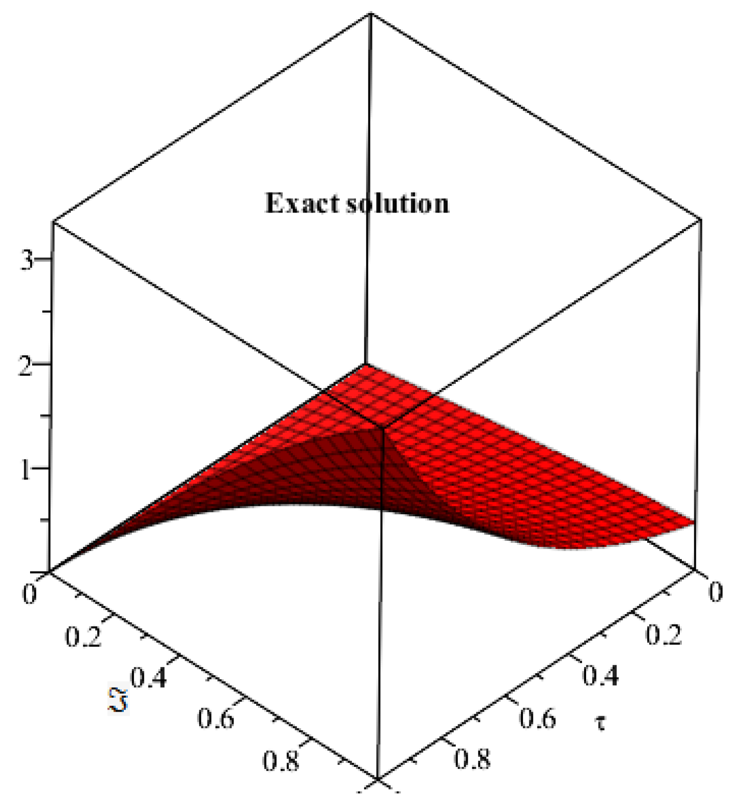
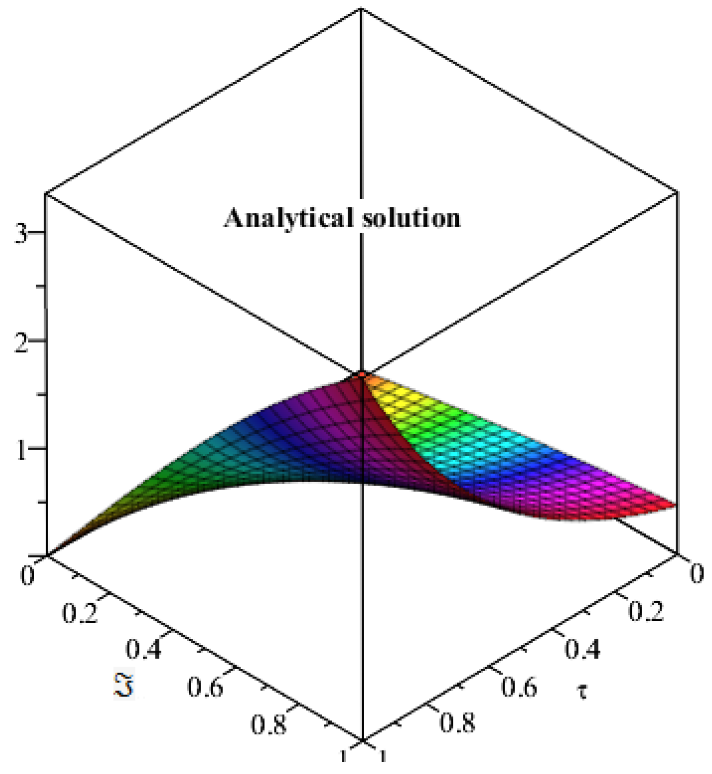
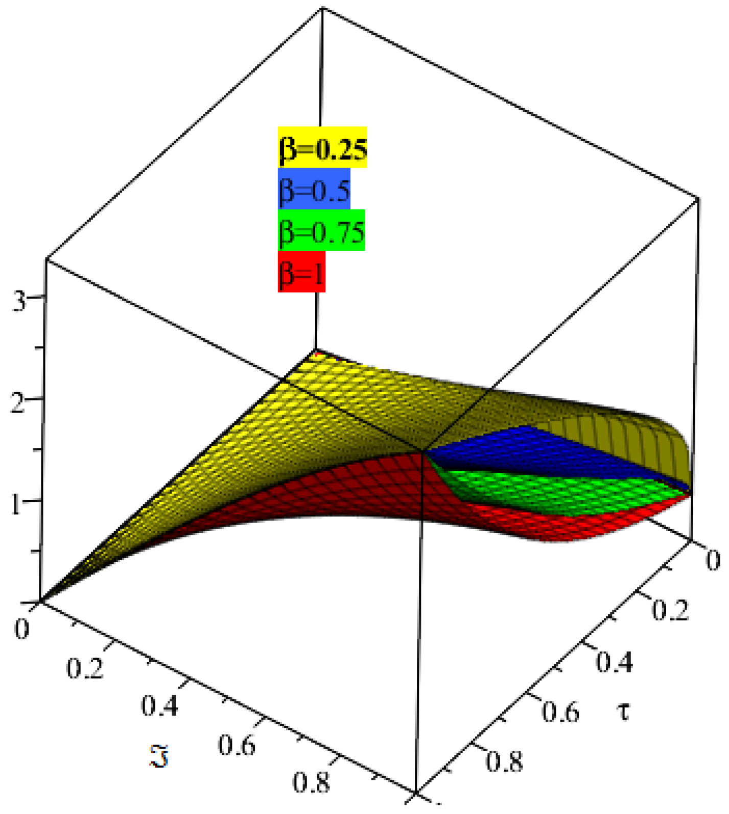
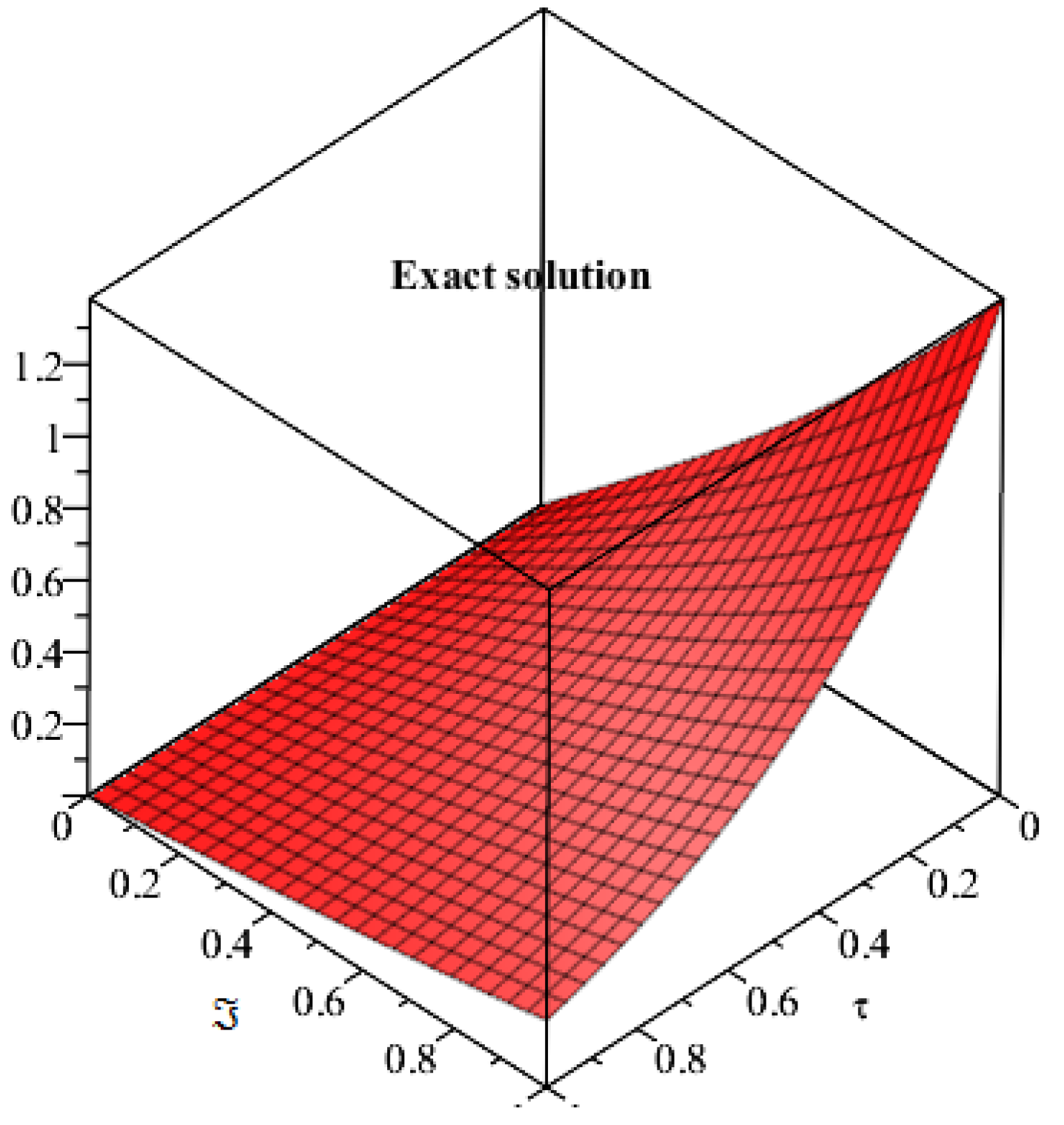
5. Results and Discussion

In the present research work, we implemented a new analytical technique SDM for the solution of some important problems which are frequently arising in science and engineering, such as hyperbolic wave equation, heat equation, diffusion equation, telegraph and Burgers equations. The Caputo definition of fractional-derivative is used to define fractional-derivative. The proposed method is the combination of Shehu transformation and Adomian decomposition method which is known as Shehu decomposition method. For applicability and novelty of present method, we applied it different physical problems for applied sciences. These problems have been solved by using SDM for both fractional and integer-order of the targeted problems. In this connection some figure analysis have been done to demonstrate the obtained results in a sophisticated manner. It is investigated that SDM solution have a very close contact with the exact solution of the problems. It is also observed that the fractional-order problems are convergent towards the solution of an integer-order problem. Moreover, the high rate of convergence of the current method is noted during the simulation. It is calculated that the SDM can be considered as one of the best analytical technique to solve fractional partial differential equations.

6. Conclusions

In the present article, we presented some fractional-view analysis of physical problems, arising in science and engineering. A new and sophisticated analytical technique, which is known as Shehu transform decomposition method is implemented for both fractional and integer-orders of the problems. The Caputo definition of fractional derivative is used to express fractional-order derivative. For applicability and reliability of the proposed methods, some illustrative examples are presented from different areas of applied science. It has been investigated through graphical representation that the present technique provides an accurate and deserving analysis about the physical happening of the problems. It is observed through simulations of the present algorithm that as fractional-order of the derivative approaches to integer order of the problem then fractional-order solutions are convergent to integer-order solutions. Moreover, the present method is preferred as compared to other method because of its better rate of convergence. This direction motivates the researchers towards the implementation of the current method for other non-linear fractional partial differential equations.

Author Contributions

Conceptualization, R.S. and H.K.; Methodology, M.A.; Software, R.S.; Validation, R.S. and U.F.; Formal Analysis, R.S.; Investigation, R.S. and D.B.; Resources, H.K. and P.K.; Writing—Original Draft Preparation, R.S.; Writing—Review and Editing, H.K., U.F. and P.K.; Visualization, M.A.; Supervision, D.B., P.K.; Project Administration, P.K.; Funding Acquisition, P.K. All authors have read and agreed to the published version of the manuscript.

Funding

Center of Excellence in Theoretical and Computational Science (TaCS-CoE) Faculty of Science, King Mongkuts University of Technology Thonburi (KMUTT).

Conflicts of Interest

The authors declare no conflict of interest.

References

  1. Abd-Elhameed, W.M.; Youssri, Y.H. Fifth-kind orthonormal Chebyshev polynomial solutions for fractional differential equations. Comput. Appl. Math. 2018, 37, 2897–2921. [Google Scholar] [CrossRef]
  2. Shah, R.; Khan, H.; Farooq, U.; Baleanu, D.; Kumam, P.; Arif, M. A New Analytical Technique to Solve System of Fractional-Order Partial Differential Equations. IEEE Access 2019, 7, 150037–150050. [Google Scholar] [CrossRef]
  3. Jain, S. Numerical analysis for the fractional diffusion and fractional Buckmaster equation by the two-step Laplace Adam-Bashforth method. Eur Phys. J. Plus 2018, 133, 19. [Google Scholar] [CrossRef]
  4. Prakash, A. Analytical method for space-fractional telegraph equation by homotopy perturbation transform method. Nonlinear Eng. 2016, 5, 123–128. [Google Scholar] [CrossRef]
  5. Khan, H.; Shah, R.; Baleanu, D.; Kumam, P.; Arif, M. Analytical Solution of Fractional-Order Hyperbolic Telegraph Equation, Using Natural Transform Decomposition Method. Electronics 2019, 8, 1015. [Google Scholar] [CrossRef] [Green Version]
  6. Safari, M.; Ganji, D.D.; Moslemi, M. Application of He’s variational iteration method and Adomian’s decomposition method to the fractional KdV–Burgers–Kuramoto equation. Comput. Math. Appl. 2009, 58, 2091–2097. [Google Scholar] [CrossRef] [Green Version]
  7. Kumar, D.; Tchier, F.; Singh, J.; Baleanu, D. An efficient computational technique for fractal vehicular traffic flow. Entropy 2018, 20, 259. [Google Scholar] [CrossRef] [Green Version]
  8. Singh, J.; Kumar, D.; Baleanu, D.; Rathore, S. An efficient numerical algorithm for the fractional Drinfeld–Sokolov–Wilson equation. Appl. Math. Comput. 2018, 335, 12–24. [Google Scholar] [CrossRef]
  9. Shivanian, E.; Jafarabadi, A. Time fractional modified anomalous sub-diffusion equation with a nonlinear source term through locally applied meshless radial point interpolation. Mod. Phys. Lett. B 2018, 32, 1850251. [Google Scholar] [CrossRef]
  10. Ullah, S.; Khan, M.A.; Farooq, M. A new fractional model for the dynamics of the hepatitis B virus using the Caputo-Fabrizio derivative. Eur. Phys. J. Plus 2018, 133, 237. [Google Scholar] [CrossRef]
  11. Qureshi, S.; Yusuf, A. Modeling chickenpox disease with fractional derivatives: From caputo to atangana-baleanu. Chaos Solitons Fractals 2019, 122, 111–118. [Google Scholar] [CrossRef]
  12. Qureshi, S.; Yusuf, A.; Shaikh, A.A.; Inc, M.; Baleanu, D. Fractional modeling of blood ethanol concentration system with real data application. Chaos Interdiscip. J. Nonlinear Sci. 2019, 29, 013143. [Google Scholar] [CrossRef] [PubMed]
  13. Khan, M.A.; Ullah, S.; Farooq, M. A new fractional model for tuberculosis with relapse via Atangana–Baleanu derivative. Chaos Solitons Fractals 2018, 116, 227–238. [Google Scholar] [CrossRef]
  14. Jena, R.M.; Chakraverty, S. Residual Power Series Method for Solving Time-fractional Model of Vibration Equation of Large Membranes. J. Appl. Comput. Mech. 2019, 5, 603–615. [Google Scholar]
  15. Jena, R.M.; Chakraverty, S. A new iterative method based solution for fractional Black–Scholes option pricing equations (BSOPE). SN Appl. Sci. 2019, 1, 95. [Google Scholar] [CrossRef] [Green Version]
  16. Jena, R.M.; Chakraverty, S.; Jena, S.K. Dynamic response analysis of fractionally damped beams subjected to external loads using homotopy analysis method. J. Appl. Comput. Mech. 2019, 5, 355–366. [Google Scholar]
  17. Abd-Elhameed, W.M.; Youssri, Y.H. Spectral tau algorithm for certain coupled system of fractional differential equations via generalized Fibonacci polynomial sequence. Iran. J. Sci. Technol. Trans. A Sci. 2019, 43, 543–554. [Google Scholar] [CrossRef]
  18. Khan, H.; Shah, R.; Kumam, P.; Arif, M. Analytical Solutions of Fractional-Order Heat and Wave Equations by the Natural Transform Decomposition Method. Entropy 2019, 21, 597. [Google Scholar] [CrossRef] [Green Version]
  19. Shah, R.; Khan, H.; Mustafa, S.; Kumam, P.; Arif, M. Analytical Solutions of Fractional-Order Diffusion Equations by Natural Transform Decomposition Method. Entropy 2019, 21, 557. [Google Scholar] [CrossRef] [Green Version]
  20. Khan, M.A.; Ullah, S.; Okosun, K.O.; Shah, K. A fractional order pine wilt disease model with Caputo–Fabrizio derivative. Adv. Differ. Equ. 2018, 2018, 410. [Google Scholar] [CrossRef]
  21. Singh, J.; Kumar, D.; Baleanu, D. On the analysis of fractional diabetes model with exponential law. Adv. Differ. Equ. 2018, 2018, 231. [Google Scholar] [CrossRef] [Green Version]
  22. Qureshi, S.; Yusuf, A. Mathematical modeling for the impacts of deforestation on wildlife species using Caputo differential operator. Chaos Solitons Fractals 2019, 126, 32–40. [Google Scholar] [CrossRef]
  23. Jumarie, G. Laplace’s transform of fractional order via the Mittag–Leffler function and modified Riemann–Liouville derivative. Appl. Math. Lett. 2009, 22, 1659–1664. [Google Scholar] [CrossRef] [Green Version]
  24. Kumar, S. A new analytical modelling for fractional telegraph equation via Laplace transform. Appl. Math. Model. 2014, 38, 3154–3163. [Google Scholar] [CrossRef]
  25. Kazem, S. Exact solution of some linear fractional differential equations by Laplace transform. Int. J. Nonlinear Sci. 2013, 16, 3–11. [Google Scholar]
  26. Namias, V. The fractional order Fourier transform and its application to quantum mechanics. IMA J. Appl. Math. 1980, 25, 241–265. [Google Scholar] [CrossRef]
  27. Chen, C.M.; Liu, F.; Turner, I.; Anh, V. A Fourier method for the fractional diffusion equation describing sub-diffusion. J. Comput. Phys. 2007, 227, 886–897. [Google Scholar] [CrossRef] [Green Version]
  28. Jiang, X.; Xu, M. The fractional finite Hankel transform and its applications in fractal space. J. Phys. A Math. Theor. 2009, 42, 385201. [Google Scholar] [CrossRef]
  29. Gorenflo, R.; Iskenderov, A.; Luchko, Y. Mapping between solutions of fractional diffusion-wave equations. Fract. Calculus Appl. Anal. 2000, 3, 75–86. [Google Scholar]
  30. Debnath, L.; Bhatta, D. Integral Transforms and Their Applications; Chapman and Hall/CRC: Boca Raton, FL, USA, 2014. [Google Scholar]
  31. Yang, X.J. Local Fractional Functional Analysis and Its Applications; Asian Academic Publisher Limited: Hong Kong, China, 2011. [Google Scholar]
  32. Neamaty, A.; Agheli, B.; Darzi, R. Applications of homotopy perturbation method and Elzaki transform for solving nonlinear partial differential equations of fractional order. Theory Approx. Appl. 2016, 6, 91–104. [Google Scholar]
  33. Jena, R.M.; Chakraverty, S. Solving time-fractional Navier–Stokes equations using homotopy perturbation Elzaki transform. SN Appl. Sci. 2019, 1, 16. [Google Scholar] [CrossRef] [Green Version]
  34. Taha, N.E.H.; Nuruddeen, R.I.; Abdelilah, K.; Hassan, S. Dualities between “Kamal and Mahgoub integral transforms” and “Some famous integral transforms”. Br. J. Appl. Sci. Technol. 2017, 20, 1–8. [Google Scholar] [CrossRef]
  35. Aboodh, K.S. The new integral transform “Aboodh Transform”. Glob. J. Pure Appl. Math. 2013, 9, 35–43. [Google Scholar]
  36. Aggarwal, S.; Chauhan, R. A comparative study of Mohand and Aboodh transforms. Int. J. Res. Adv. Technol. 2019, 7, 520–529. [Google Scholar] [CrossRef]
  37. Kılıçman, A.; Gadain, H.E. On the applications of Laplace and Sumudu transforms. J. Frankl. Inst. 2010, 347, 848–862. [Google Scholar] [CrossRef]
  38. Jena, R.M.; Chakraverty, S. Analytical solution of Bagley-Torvik equations using Sumudu transformation method. SN Appl. Sci. 2019, 1, 246. [Google Scholar] [CrossRef] [Green Version]
  39. Mao, Z.; Shen, J. Hermite spectral methods for fractional PDEs in unbounded domains. SIAM J. Sci. Comput. 2017, 39, A1928–A1950. [Google Scholar] [CrossRef]
  40. Maitama, S.; Zhao, W. New integral transform: Shehu transform a generalization of Sumudu and Laplace transform for solving differential equations. arXiv 2019, arXiv:1904.11370. [Google Scholar]
  41. Rudolf, H. (Ed.) Applications of Fractional Calculus in Physics; World Scientific: Singapore, 2000. [Google Scholar]
  42. Wazwaz, A.M.; Gorguis, A. Exact solutions for heat-like and wave-like equations with variable coefficients. Appl. Math. Comput. 2004, 149, 15–29. [Google Scholar] [CrossRef]
Figure 1. Represents the exact solution of Example 1 at β = 2 .
Applsci 10 00122 g001
Figure 2. Represents the analytical solution of Example 1 at β = 2 .
Applsci 10 00122 g002
Figure 3. Represents the solution at different fractional order of Example 1.
Applsci 10 00122 g003
Figure 4. Represents the solution at different fractional order of Example 1.
Applsci 10 00122 g004
Figure 5. Represents the exact solution of Example 2 at β = 1 .
Applsci 10 00122 g005
Figure 6. Represents the analytical solution of Example 2 at β = 1 .
Applsci 10 00122 g006
Figure 7. u ( , , τ ) Represents the solution at different fractional order of Example 2.
Applsci 10 00122 g007
Figure 8. u ( , , τ ) Represents the solution at different fractional order of Example 2.
Applsci 10 00122 g008
Figure 9. Exact solution of Example 3 at β = 1 .
Applsci 10 00122 g009
Figure 10. Represents the analytical solution of Example 3 at β = 1 .
Applsci 10 00122 g010
Figure 11. The solution graph at different fractional order β .
Applsci 10 00122 g011
Figure 12. Exact solution of Example 4 at β = 2 .
Applsci 10 00122 g012
Figure 13. Analytical solution of Example 4 at β = 2 .
Applsci 10 00122 g013
Figure 14. The solution graph at different fractional order β . of Example 4.
Applsci 10 00122 g014
Figure 15. Exact solution of Example 5 at β = 1 .
Applsci 10 00122 g015
Figure 16. Represents the analytical solution of Example 5 at β = 1 .
Applsci 10 00122 g016
Figure 17. The solution of fractional-order β = 0 . 75 of Example 5.
Applsci 10 00122 g017
Figure 18. The solution of fractional-order β = 0 . 5 of Example 5.
Applsci 10 00122 g018
Table 1. The Shehu transform of some special functions.
Functional FormShehu Transform Form
1 u s
t u 2 s 2
e τ u s a u
sin ( τ ) u 2 s 2 + u 2
cos ( τ ) u s s 2 + u 2
τ n n ! for n = 0 , 1 , 2 , ( u s ) n + 1
τ n Γ ( n + 1 ) for n = 0 , 1 , 2 , ( u s ) n + 1
Table 2. Comparison of SDM and ADM [42] of Example 1 at τ = 0 . 1 .
SDM (m = 5)SDM (m = 3)SDM ( m= 5)ADM (m = 5)AE of SDM
β = 1 . 75 β = 2 β = 2 β = 2 β = 2
111.1115689741.1051958331.105196081.105196092.51 × 10 5
2217.7851035817.6831333317.683137317.68313744.02 × 10 4
3390.0370868889.5208625089.520882989.52088282.03 × 10 3
44284.5616573282.9301334282.930198282.9301996.44 × 10 3
55694.7306086690.7473959690.747553690.7475521.57 × 10 2

