Ambient Air Quality Assessment in Blantyre Malawi Using Low-Cost Sensors

Abstract

This study presents an assessment of ambient air quality in Chichiri and Malawi University of Business and Applied Sciences (MUBAS) locations, Blantyre City, Southern Malawi. The study aimed at assessing temporal trends, identifying exceedance of thresholds, investigating relationships between pollutants and meteorological factors, and exploring the predictability of air quality index (AQI). Five pollutants: ${\mathrm{P}\mathrm{M}}_{2.5}$, ${\mathrm{P}\mathrm{M}}_{10}$, ${\mathrm{N}\mathrm{O}}_{\mathrm{x}}$, ${\mathrm{C}\mathrm{O}}_2$ and TVOC were assessed over a two-month period using fixed low-cost sensors. Daily and hourly temporal analysis showed that pollutants peak during morning and evening hours. A significant number of exceedances for ${\mathrm{P}\mathrm{M}}_{2.5}$ and ${\mathrm{P}\mathrm{M}}_{10}$ were observed when compared to indicative thresholds. Chichiri exhibited more frequent AQI classifications in the “unhealthy” range. A strong positive relationship between ${\mathrm{P}\mathrm{M}}_{2.5}$ and ${\mathrm{P}\mathrm{M}}_{10}$ (r $=$ 0.84) and positive correlations between ${\mathrm{N}\mathrm{O}}_{\mathrm{x}}$ and ${\mathrm{C}\mathrm{O}}_2$ were observed. A multiple linear regression model achieved a high coefficient of determination (${\mathrm{R}}^2$ $=$ 0.938), identifying ${\mathrm{P}\mathrm{M}}_{10}$ and ${\mathrm{N}\mathrm{O}}_{\mathrm{x}}$ as dominant predictors of AQI variability. Temperature and humidity showed modest inverse relationship with AQI, suggesting dispersion effects. A comparison with African cities showed that the study areas’ pollution levels were within regional norms, but that there is a need for targeted mitigation. These findings underscore the importance of continuous monitoring, data-driven policy making and regional collaboration to address urban air quality challenges.

1. Introduction

Pollution is a problem that the world has been grappling with since the industrial revolution. Air pollution has been receiving attention for decades but not at par with water pollution. This is very worrisome as 90% of individuals breathe air which contains polluted compounds presenting a risk to human health [1]. In fact, according to the World Health Organization (WHO), each year, 7 million people die due to air pollution [2,3]. Every day, people encounter air pollutants unwittingly, often oblivious to the substantial adverse impacts these can have on their health [4]. In Malawi, air pollution comes from multiple sources which include vehicle emissions, industrial emissions, dust, and the use of biomass as a source of energy, among many other sources [5,6,7,8].

Air pollution is not only a risk to human health, but it also affects other organisms. The risks that air pollution poses to human health and the well-being of other organisms worldwide have drawn a lot of attention lately [9]. Air pollutants have been implicated in hampering human development aspects [10]. This is apart from other effects ranging from minor upper respiratory irritation to chronic respiratory and heart disease, lung cancer, acute respiratory infections in children and chronic bronchitis in adults, aggravating pre-existing heart and lung disease, or asthmatic attacks [11]. Additionally, short- and long-term exposures have also been linked to premature mortality and reduced life expectancy. Studies have shown that students studying in schools located in environmentally polluted areas (including air pollution) exhibit attention, thinking and decision-making abilities consistent with cognitive function impairment [12]. Individuals inhabiting areas with high levels of air pollution have markers of neuroinflammation and neuropathology that are associated with neurodegenerative conditions such as Alzheimer’s disease-like brain pathologies [13]. Overall, air pollution is a leading cause of global morbidity and mortality, and an important driver of health inequalities [14,15].

Monitoring of air pollutants is very important as it is a step towards their control. The biggest challenge with air pollutants is that they disperse very easily from the point of generation, often carried away by the wind. This has made emission abatement measures tricky [16]. The pollution abatement measures must target the right emission sources for them to be effective, however, primary pollutants (which can easily be abated), react to form secondary air pollutants which become difficult to control [17]. The formation of secondary pollutants has made it possible to have thousands of air pollutants in the atmosphere [18].

Ambient air pollutant measurements have been done in a number of countries. For example, in the United States, Padilla [19] found that ambient measurements of hazardous air pollutants routinely exceed predictions from screening-level exposure models. In China, studies have implicated industrialization and urbanization as the major causes of ambient air pollution [20,21]. According to Sengani [22], coastal development induces industrialization and urbanization such that in their study conducted in India around the coast of Gujarat, it was found that in most of the sampled stations, the particulate matter fractions exceeded the National Ambient Air Quality Standard (NAAQS). In the United Kingdom, a review by Goddard [23] found that the concentration of metals in air is on the decline. In Egypt, Elawa [24] found that particulate matter was high around 21 studied sites around cement production companies. The particulate matter was attributed to raw materials mining, transportation, blending, quarrying, preparation, and stockpiles in the cement production areas.

In most developed countries, high-tech monitoring equipment is utilized to measure and study air quality, which is not the case in developing countries. Many researchers in developing nations now employ satellite-based sensors to monitor the ambient air quality [9]. The satellite-generated data may not be very accurate as compared to using air quality monitors deployed in target areas of interest. It is for this reason that the major aim of this study was to assess the ambient air quality in Blantyre, Malawi, using fixed low-cost sensors. Air pollution in Malawi is recognized as one of the key environmental issues ranking eighth out of nine key priority areas [25]. Accordingly, this assessment is not only very important to the country but also the region, as air pollutants tend to disperse. Measuring and evaluating environmental levels of air pollution is a step toward protecting public health [26]. In the previous studies [27,28], it was shown that the air quality in Malawi can be explained using ground-based truth data, and that the main challenge still remains, which is having real time continuous monitoring of air quality.

This study has focused on understanding the concentrations of key pollutants, namely, ${\mathrm{P}\mathrm{M}}_{2.5}$ (particulate matter with aerodynamics diameter $\le$ 2.5 μm$)$, ${\mathrm{P}\mathrm{M}}_{10}$ (particulate matter with aerodynamics diameter $\le$ 10 μm), ${\mathrm{N}\mathrm{O}}_{\mathrm{x}}$ (nitrogen oxides), ${\mathrm{C}\mathrm{O}}_2$ (carbon dioxide) and TVOC (total volatile organic compounds) over a two-month period using fixed low-cost sensors from AirGradient Company. These pollutants impact human health, negatively affect urban sustainability and destroy ecosystems. The research also bridges the gap of low systematic air quality monitoring in Malawi, taking advantage of the usage of low-cost real-time monitoring sensors. By integrating pollutant exceedance detection, Air Quality Index (AIQ) classifications and a simplified regression model, this study provides a comprehensive baseline for urban air quality in Malawi.

2. Materials and Methods

2.1. The Study Area

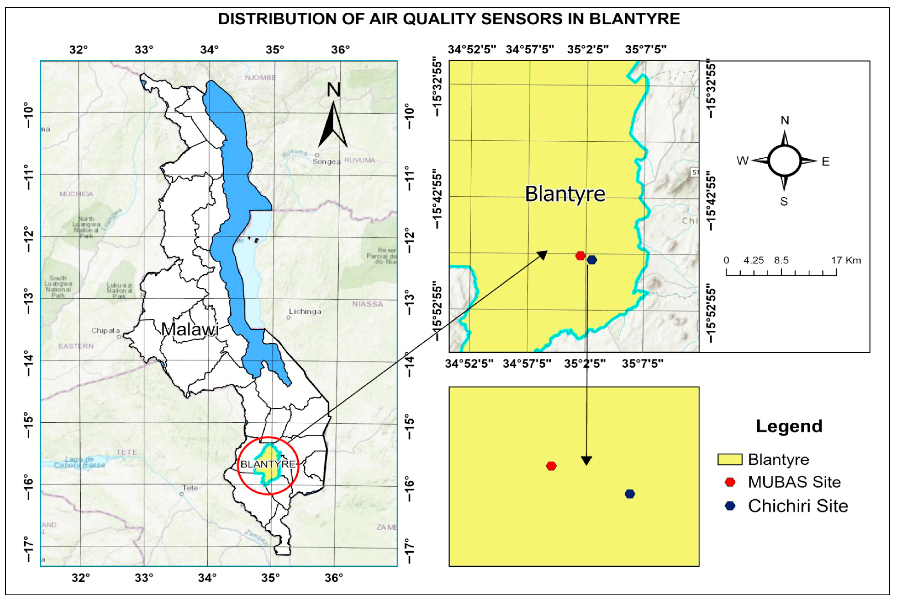
This study investigated ambient air quality for two sites in Blantyre, Malawi. The sites were Chichiri (which lies at 15°48′27″, 35°02′36″) and Malawi University of Business and Applied Sciences (MUBAS) (which lies at 15°48′06″ S, 35°01′37″ E). The two sites are roughly 2.5 km apart and Figure 1 is a map of the study area. These locations were selected due to their proximity to traffic corridors, residential combustion sources, and high commercial activities. For example, the Chipembere Highway (a very busy route, https://www.google.com/maps/place/Masauko+Chipembere+Hwy,+Blantyre,+Malawi/@-15.8012371,35.0313222,1046m/data=!3m2!1e3!4b1!4m6!3m5!1s0x18d84597ee03e45f:0x2f581c075f0b4bbb!8m2!3d-15.8012371!4d35.0338971!16s%2Fg%2F11ff5p9d9d?entry=ttu&g_ep=EgoyMDI1MTIwMi4wIKXMDSoASAFQAw%3D%3D, accessed on 20 December 2025) passes through the MUBAS (https://www.google.com/maps/search/Malawi+University+of+Business+and+Applied+Sciences+MUBAS/@-15.8039151,35.0206186,4082m/data=!3m1!1e3?entry=ttu&g_ep=EgoyMDI1MTIwMi4wIKXMDSoASAFQAw%3D%3D, accessed on 20 December 2025) site. On the other hand, the Chichiri site is a residential area very close to Maselema Industrial Area (https://www.google.com/maps/search/maselema/@-15.80216,35.0489756,838m/data=!3m2!1e3!4b1?entry=ttu&g_ep=EgoyMDI1MTIwMi4wIKXMDSoASAFQAw%3D%3D, accessed on 20 December 2025) and also two busy routes (Masauko Chipembere Highway and Kanjedza By-pass Road (https://www.google.com/maps/search/Kanjedza+Road,+Blantyre,+Republic+of+Malawi/@-15.8083396,35.0430536,419m/data=!3m1!1e3?entry=ttu&g_ep=EgoyMDI1MTIwMi4wIKXMDSoASAFQAw%3D%3D, accessed on 20 December 2025)) pass through this area.

2.2. Data Collection

Data were collected from 8 August 2025 to 8 October 2025, using air quality monitors mounted on stands and installed on rooftops (at a minimum of 1.5 m above the roof surface) (Figure 2). The air quality monitors (AirGradient Open Air Max; Model: O-M-1PPST-CE, running on firmware version 0.5.1) manufactured by AirGradient Company Limited, Chiang Mai, Thailand were equipped with solar panels and a provision for 4G/GSM sim cards. The instrument calibration was done by AirGradient using the EPA Calibration Algorithm (PMS5003_20240826). The devices were operated on a local network and data were retrieved from a computer system hosted by AirGradient. Real-time monitoring data are available on an interactive map which at the time of writing this manuscript, could be accessed at the following link (https://www.airgradient.com/map, accessed on 20 December 2025). These data are also accessible through the OpenAQ (https://explore.openaq.org/#1.2/20/40, accessed on 20 December 2025). Data for air quality (${\mathrm{P}\mathrm{M}}_{2.5}$, ${\mathrm{P}\mathrm{M}}_{10}$, ${\mathrm{N}\mathrm{O}}_{\mathrm{x}}$, ${\mathrm{C}\mathrm{O}}_2$ and TVOC) were collected at sub-hourly intervals and retrieved in CSV format from the monitors, then processed using a modular python workflow. Meteorological variables were also retained for correlation and source inference analyses. For ${\mathrm{N}\mathrm{O}}_{\mathrm{x}}$ and TVOC values, the raw data were converted using factors of 0.02 and 10 $\mathsf{\mu }\mathrm{g}/{\mathrm{m}}^3$ respectively, to align them with WHO/International Air Quality (IAQ) guidelines.

2.3. Determination of the Diurnal Temporal Trends of Ambient Pollutants

The first stage of the research was a study of the temporal trends of the selected ambient pollutants, ${\mathrm{P}\mathrm{M}}_{2.5}$, ${\mathrm{P}\mathrm{M}}_{10}$, ${\mathrm{N}\mathrm{O}}_{\mathrm{x}}$, ${\mathrm{C}\mathrm{O}}_2$ and TVOC, at both daily and hourly resolution. Daily average concentrations for each pollutant were calculated by grouping the combined data-frame by date and location, and then computing the mean for the specified pollutant. Similarly, diurnal average concentrations were calculated by grouping the data frame by hour and location, and then computing the mean for a particular pollutant. A 1 -hour rolling average was applied to these mean values using the rolling method with a window size of 3 and mindash–periods of 1. This was applied after grouping the data by location to smooth the diurnal profiles. To examine potential differences in pollutant levels between weekdays (Monday through Friday) and weekends (Saturday and Sunday), box plots were made for each pollutant and location using matplotlib. These distinctions were included to see the influence of short-term pollution patterns, since the two study sites experience differences in traffic volume, commercial activity, and human mobility between weekdays and weekends. The simple moving average (SMA) for a time series data point ${\mathrm{P}}_{\mathrm{t}}$ with a window size $\mathrm{n}$ was calculated using Equation (1).

$${\mathrm{S}\mathrm{M}\mathrm{A}}_{\mathrm{t}}={\displaystyle \frac{1}{\mathrm{n}}}\sum _{\mathrm{i}-\mathrm{t}-\mathrm{n}+1}^{\mathrm{t}}{\mathrm{P}}_{\mathrm{i}}$$

(1)

where ${\mathrm{P}}_{\mathrm{i}}$ represents data points within the window.

2.4. Analysis of Exceedance Detection and AQI Classification

This study also included analysis of exceedance detection and AQI classification, to identify instances where pollutant concentrations exceeded pre-defined thresholds.

2.4.1. Exceedance Detection

Pollutant exceedances were flagged using thresholds based on WHO guidelines [29] and outdoor air quality literature [30].

Table 1. Threshold pollutants.

Parameter	Value (Unit)	Scale
${\mathrm{P}\mathrm{M}}_{2.5}$	25 $\mathsf{\mu }\mathrm{g}/{\mathrm{m}}^3$	24 h mean
${\mathrm{P}\mathrm{M}}_{10}$	50 $\mathsf{\mu }\mathrm{g}/{\mathrm{m}}^3$	24 h mean
${\mathrm{N}\mathrm{O}}_{\mathrm{x}}$	200 $\mathsf{\mu }\mathrm{g}/{\mathrm{m}}^3$	1 h mean
${\mathrm{C}\mathrm{O}}_2$	1000 ppm	Comfort threshold for indoor air
TVOC	500	IAQ guideline, sensor-scaled

shows the thresholds used in this work.

Each pollutant was assigned a binary exceedance flag ${\mathrm{E}}_{\mathrm{P}}\left(\mathrm{t}\right)$ at time $\mathrm{t}$ computed following Equation (2).

$${\mathrm{E}}_{\mathrm{p}}\left(\mathrm{t}\right)=\left\{\begin{array}{c}1\\ 0\end{array}\right.{\displaystyle \genfrac{}{}{0pt}{}{\mathrm{i}\mathrm{f} {\mathrm{C}}_{\mathrm{P}}\left(\mathrm{t}\right)>{\mathrm{T}}_{\mathrm{p}}}{\mathrm{o}\mathrm{t}\mathrm{h}\mathrm{e}\mathrm{r}\mathrm{w}\mathrm{i}\mathrm{s}\mathrm{e}}}$$

(2)

where ${\mathrm{C}}_{\mathrm{P}}\left(\mathrm{t}\right)$ is the measured concentration, and ${\mathrm{T}}_{\mathrm{p}}$ is the threshold.

2.4.2. Air Quality Index Computation

The AQI values for the pollutants were computed using a piecewise linear function based on pre-defined breakpoints (U.S EPA’s AQI calculation) [31]. For each pollutant, the AQI sub-index ${\mathrm{I}}_{\mathrm{P}}$ was calculated through Equation (3).

$${\mathrm{I}}_{\mathrm{P}}={\displaystyle \frac{{\mathrm{I}}_{\mathrm{h}\mathrm{i}\mathrm{g}\mathrm{h}}-{\mathrm{I}}_{\mathrm{l}\mathrm{o}\mathrm{w}}}{{\mathrm{C}}_{\mathrm{h}\mathrm{i}\mathrm{g}\mathrm{h}}-{\mathrm{C}}_{\mathrm{l}\mathrm{o}\mathrm{w}}}}\left({\mathrm{C}}_{\mathrm{P}}-{\mathrm{C}}_{\mathrm{l}\mathrm{o}\mathrm{w}}\right)+{\mathrm{I}}_{\mathrm{l}\mathrm{o}\mathrm{w}}$$

(3)

where ${\mathrm{C}}_{\mathrm{P}}$ is the pollutant concentration, ${\mathrm{C}}_{\mathrm{h}\mathrm{i}\mathrm{g}\mathrm{h}}, {\mathrm{C}}_{\mathrm{l}\mathrm{o}\mathrm{w}}$ are the lower and upper bounds of the concentration breakpoint, and ${\mathrm{I}}_{\mathrm{h}\mathrm{i}\mathrm{g}\mathrm{h}}, {\mathrm{I}}_{\mathrm{l}\mathrm{o}\mathrm{w}}$ are the corresponding AQI index bounds.

In this study, breakpoints for ${\mathrm{P}\mathrm{M}}_{2.5}$ ($\mathsf{\mu }\mathrm{g}/{\mathrm{m}}^3$) were adopted from U.S EPA [32] and implemented as follows;

• 0–12 $\to$ AQI 0–50 (good)
• 12.1–35.4 $\to$ AQI 51–100 (moderate)
• 33.5–55.4 $\to$ AQI 101–150 (unhealthy for sensitive group)
• 55.5–150.4 $\to$ AQI 151–200 (unhealthy)
• 150.5–250.4 $\to$ AQI 201–300 (very unhealthy)
• 250.5–500.4 $\to$ AQI 301–500 (hazardous)

Also, a composite AQI was defined using Equation (4).

$${\mathrm{A}\mathrm{Q}\mathrm{I}}_{\mathrm{c}\mathrm{o}\mathrm{m}\mathrm{p}\mathrm{o}\mathrm{s}\mathrm{i}\mathrm{t}\mathrm{e}}\left(\mathrm{t}\right)=\max ({\mathrm{I}}_{{\mathrm{P}\mathrm{M}}_{2.5}}\left(\mathrm{t}\right),{\mathrm{I}}_{{\mathrm{P}\mathrm{M}}_{10}}\left(\mathrm{t}\right),{\mathrm{I}}_{{\mathrm{N}\mathrm{O}}_{\mathrm{x}}}\left(\mathrm{t}\right),{\mathrm{I}}_{{\mathrm{C}\mathrm{O}}_2}$$

(4)

2.5. Correlation and Source Inference

To investigate the relationship between different pollutants and meteorological variables, a correlation analysis was performed. Temperature ($\mathrm{℃}$) and humidity (%) were the meteorological variables used due to their availability from the database, alongside the pollutants. The Pearson correlation coefficient ($\mathsf{\rho }\mathrm{X},\mathrm{Y}$) was computed between all pairs of these selected variables. This relationship between variables was calculated as

$$\mathsf{\rho }\mathrm{X},\mathrm{Y}={\displaystyle \frac{\mathrm{c}\mathrm{o}\mathrm{v}(\mathrm{X},\mathrm{Y})}{{\mathsf{\sigma }}_{\mathrm{X}}.{\mathsf{\sigma }}_{\mathrm{Y}}}}$$

(5)

where $\mathrm{c}\mathrm{o}\mathrm{v}\left(\mathrm{X},\mathrm{Y}\right)$ is the covariance between variable $\mathrm{X}$ and $\mathrm{Y}$, and ${\mathsf{\sigma }}_{\mathrm{X}}$ and ${\mathsf{\sigma }}_{\mathrm{Y}}$ are the standard deviations of $\mathrm{X}$ and $\mathrm{Y}$, respectively. The correlation coefficient ranges from $-1$ (perfect negative correlation) to $+1$ (perfect positive correlation), with $0$ indicating no correlation at all. A heatmap was used to visualize inter-variable relationships. Strong ${\mathrm{P}\mathrm{M}}_{2.5}$–${\mathrm{P}\mathrm{M}}_{10}$ correlation suggested shared sources (e.g., dust), while ${\mathrm{N}\mathrm{O}}_{\mathrm{x}}$–${\mathrm{C}\mathrm{O}}_2$ correlation indicated traffic emissions. TVOC–temperature correlation implied volatilizations or outdoor chemical activities.

2.6. Analysis of Multiple Linear Regression for AQI Prediction

A multiple linear regression analysis was conducted to model and predict the composite AQI based on the concentrations of various pollutants and meteorological variables. The composite AQI was used, where the predictor variables were the pollutants as well as meteorological parameters. Equation (6) was used as a model for the multiple linear regression.

$$\mathrm{Y}={\mathsf{\beta }}_0+{\mathsf{\beta }}_1{\mathrm{X}}_1+{\mathsf{\beta }}_2{\mathrm{X}}_2+\dots +{\mathsf{\beta }}_{\mathrm{p}}{\mathrm{X}}_{\mathrm{p}}+\mathsf{ϵ}$$

(6)

where $\mathrm{Y}$ is the target variable (composite AQI), ${\mathrm{X}}_1$, ${\mathrm{X}}_2$, … ${\mathrm{X}}_{\mathrm{p}}$ are the predictor variables, ${\mathsf{\beta }}_0$ is the intercept, ${\mathsf{\beta }}_1$, ${\mathsf{\beta }}_2$, …, ${\mathsf{\beta }}_{\mathrm{p}}$ are the regression coefficients representing the change in $\mathrm{Y}$ for a one-unit change in the corresponding predictor holding other predictors constant, and $\mathsf{ϵ}$ is the error term.

3. Results and Discussion

This section presents the key findings from the air quality analysis for this study. Temporal trends of pollutants, exceedance detection and AQI classification, correlation analysis for source inference, and multiple linear regression for AQI prediction have been provided and discussed in that order.

3.1. Diurnal Temporal Trends of Ambient Pollutants

Table 2. Results summary for Chichiri.

Analyte	Mean	Standard Deviation	Min	Max
PM2.5 (μg/m3)	59.74	41.34	0.30	323.00
PM10 (μg/m3)	65.63	42.02	0.4	333.3
NOX (μg/m3)	42.95	1.29	37.13	46.31
CO2 (ppm)	409.75	15.67	355.00	443.00
TVOC (μg/m3)	414.12	21.13	373.89	483.56
Temperature (°C)	21.67	5.64	10.70	36.50
Humidity (%)	59.56	21.33	15.00	100.00

and

Table 3. Results summary for MUBAS.

Analyte	Mean	Standard Deviation	Min	Max
PM2.5 (μg/m3)	49.24	34.91	n.d. *	264.70
PM10 (μg/m3)	54.93	36.56	0.10	276.80
NOX (μg/m3)	39.29	0.91	36.78	41.63
CO2 (ppm)	421.36	16.89	372.00	470.00
TVOC (μg/m3)	333.04	3.60	320.21	347.22
Temperature (°C)	21.80	4.63	11.50	33.90
Humidity (%)	58.08	19.51	16.00	99.00

* not detected.

summarize results over the two-month period for the Chichiri and MUBAS sites in Blantyre, Malawi. The maximum detectable values at Chichiri for PM_2.5, PM₁₀, NO_X, CO₂, TVOC, temperature and humidity were 323 μg/m³, 333 μg/m³, 46.3 μg/m³, 443 ppm, 484 μg/m³, 36.5 °C and 100.00%, respectively. The maximum detectable values at MUBAS for PM_2.5, PM₁₀, NO_X, CO₂, TVOC, temperature and humidity were 264.7 μg/m³, 276. 8 μg/m³, 41.6 μg/m³, 470 ppm, 347.2 μg/m³, 33.9 °C and 99%, respectively. Generally, the maximum values for Chichiri were higher than those of MUBAS except for CO₂.

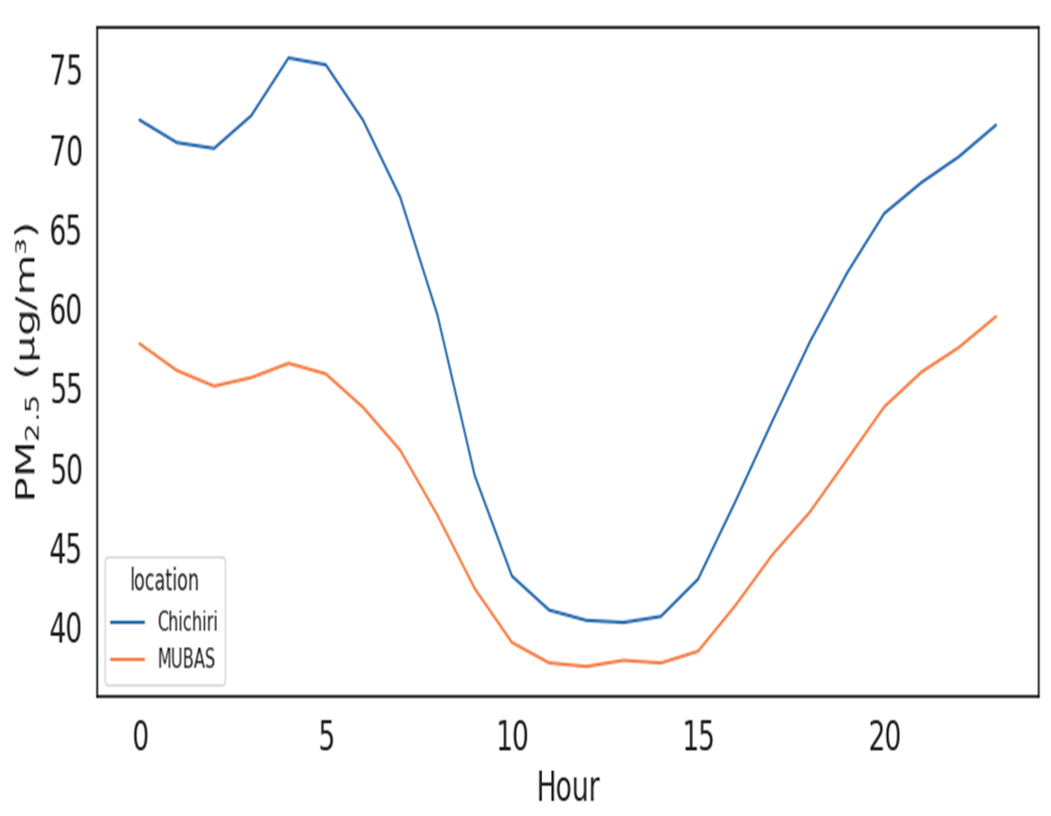
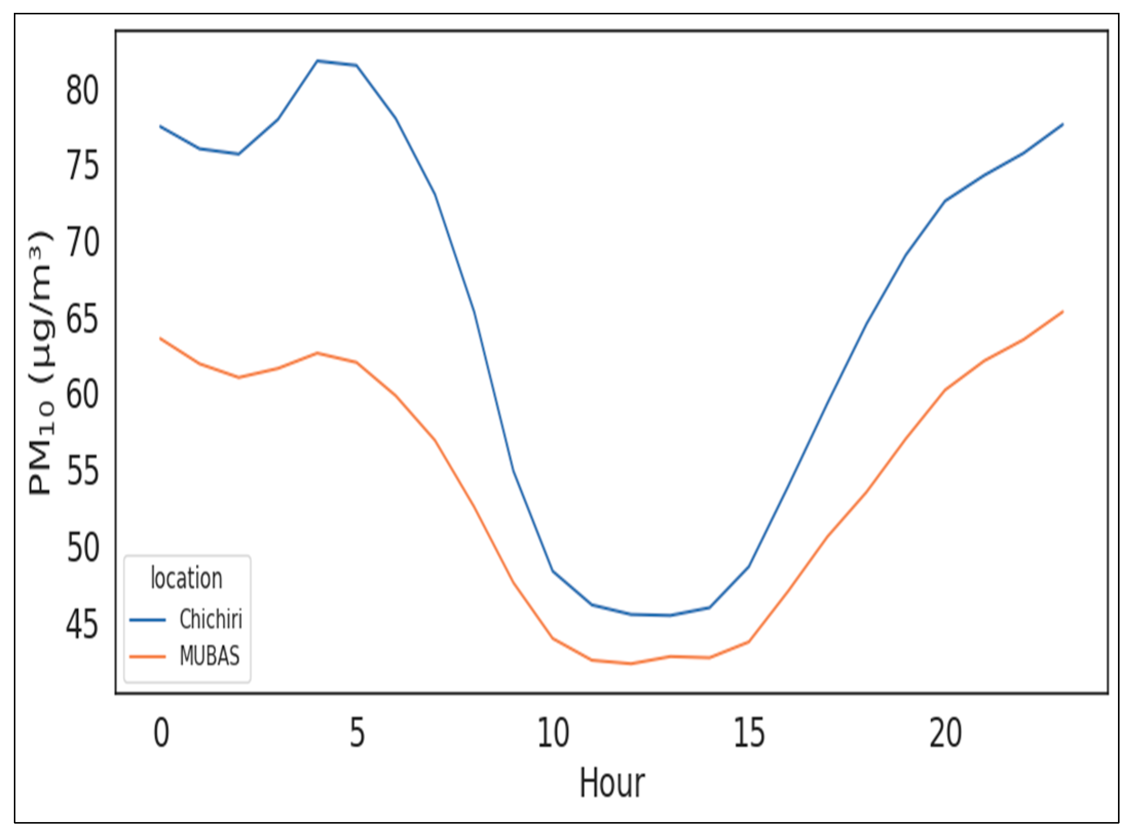
Figure 3 shows the diurnal profile of ${\mathrm{P}\mathrm{M}}_{2.5}$ concentrations, with both sites showing elevated levels during morning hours (05:00–08:00) and late evening (18:00–22:00), with a mid-day dip. These peaks align with traffic rush hours and domestic combustion activities. The mid-day dip reflects increased atmospheric mixing and reduced emissions. Chichiri recorded higher concentration, peaking near 80 $\mathsf{\mu }\mathrm{g}/{\mathrm{m}}^3$. Figure 4 shows similar trends for ${\mathrm{P}\mathrm{M}}_{10}$ with Chichiri reaching up to 90 $\mathsf{\mu }\mathrm{g}/{\mathrm{m}}^3$. Both ${\mathrm{P}\mathrm{M}}_{2.5}$ and ${\mathrm{P}\mathrm{M}}_{10}$ exceeded WHO hourly comfort thresholds, indicating acute exposure risks during peak hours. These values are similar to what was reported earlier [26] in Blantyre.

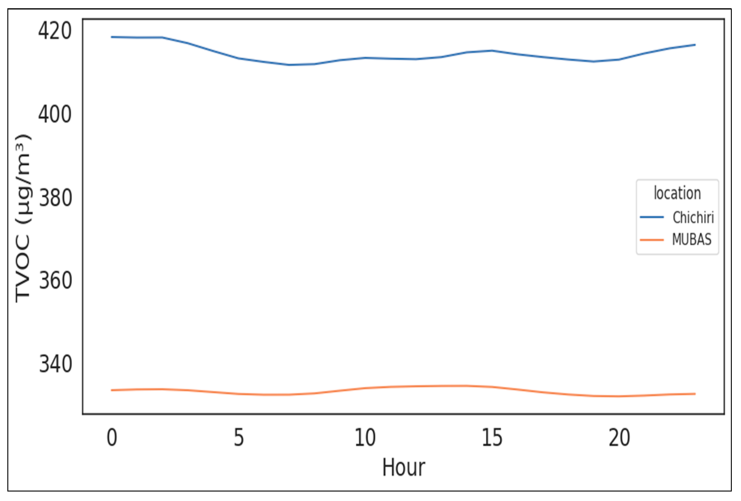
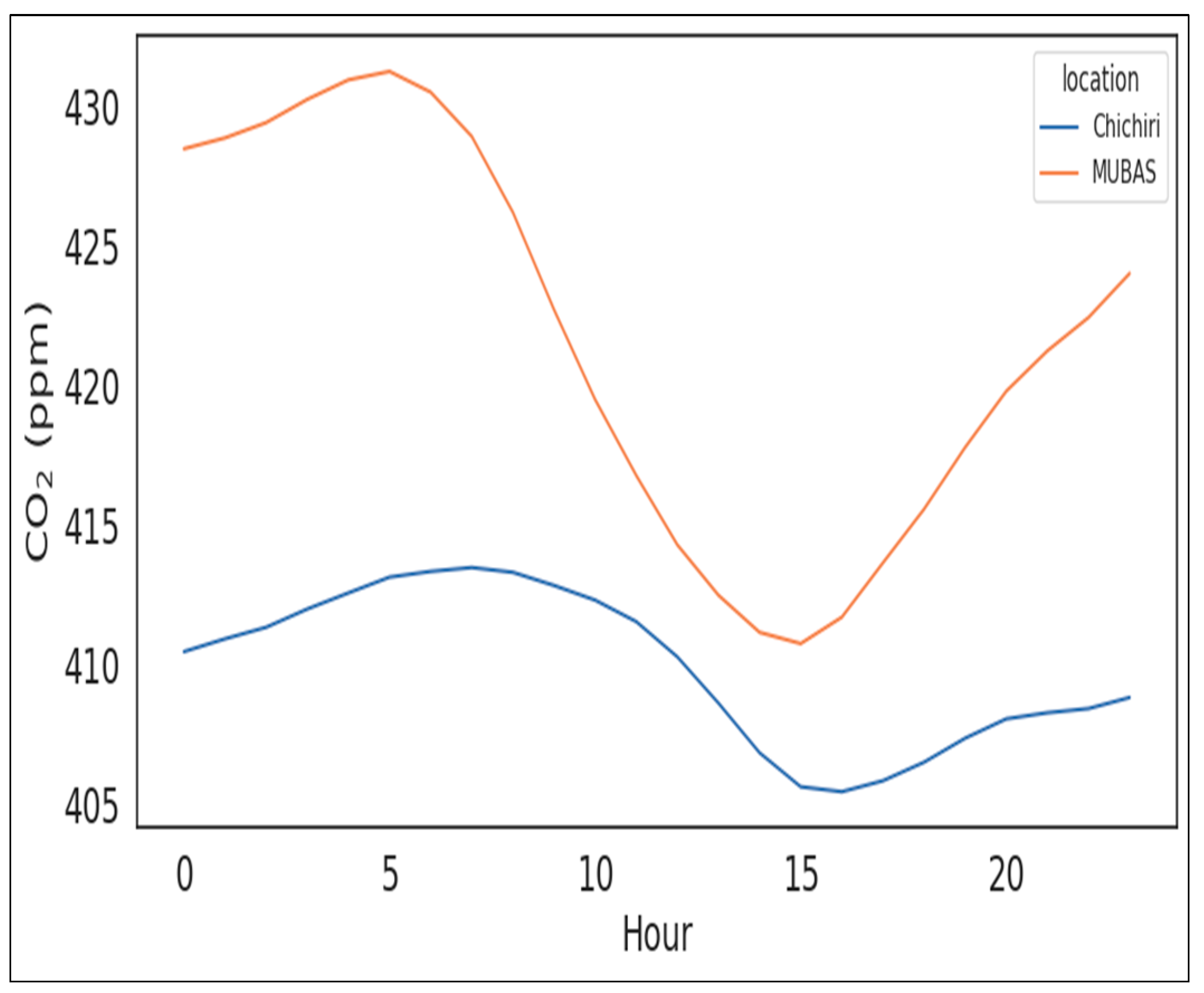
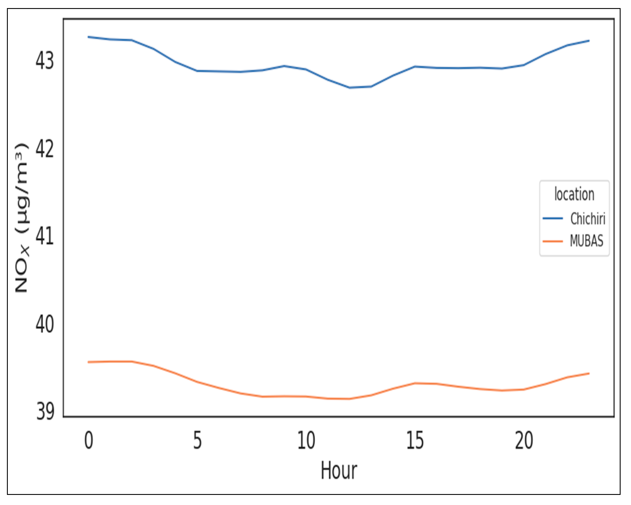
${\mathrm{C}\mathrm{O}}_2$ concentrations remained below 100 ppm during most hours (Figure 5). Morning and evening peaks are observed, which aligns with peak hours. MUBAS had higher levels, suggesting denser vehicular activity as compared to Chichiri. ${\mathrm{N}\mathrm{O}}_{\mathrm{x}}$ values (Figure 6) were too low in reference to the threshold limits and followed similar profile trends with ${\mathrm{C}\mathrm{O}}_2$. Observed low values for ${\mathrm{N}\mathrm{O}}_{\mathrm{x}}$ and ${\mathrm{C}\mathrm{O}}_2$ concentrations reinforce the role of less combustion and industrial activities in these studied areas for the monitored period. Figure 7 illustrates the hourly profile of TVOC. Chichiri starts at a higher baseline and shows a gradual decline throughout the day, while MUBAS remains stable and lower. However, below the scale’s threshold of 50,000, sustained TVOC exposure can contribute to outdoor air discomfort and respiratory irritations.

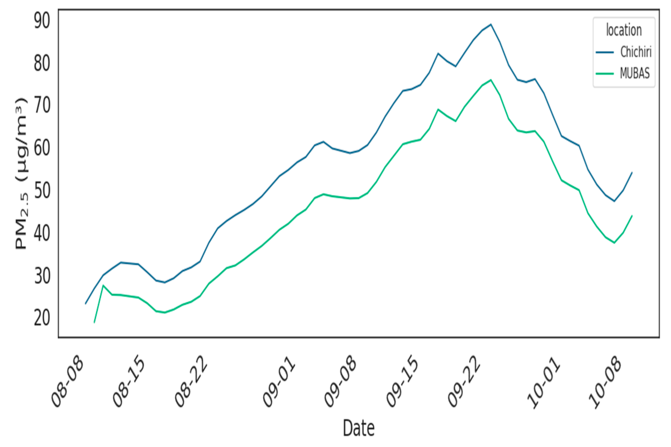
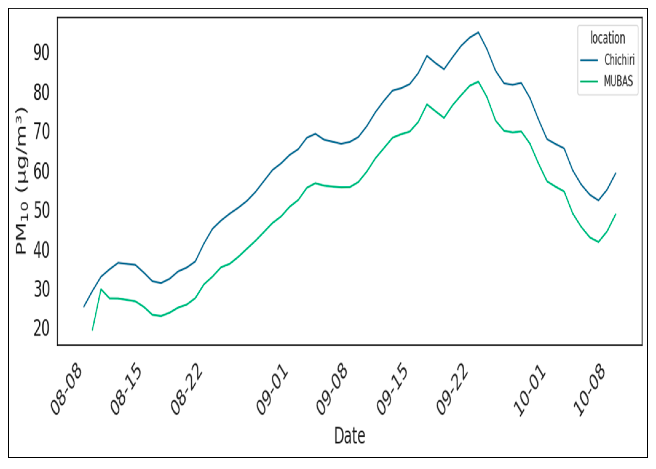
A daily concentration average of ${\mathrm{P}\mathrm{M}}_{2.5}$ and ${\mathrm{P}\mathrm{M}}_{10}$ is represented in Figure 8 and Figure 9, respectively. Again, Chichiri shows higher levels of both pollutants compared to MUBAS, with ${\mathrm{P}\mathrm{M}}_{2.5}$ peaking near 80 $\mathsf{\mu }\mathrm{g}/{\mathrm{m}}^3$ and ${\mathrm{P}\mathrm{M}}_{10}$ approaching 100 $\mathsf{\mu }\mathrm{g}/{\mathrm{m}}^3$ in late September. These high values substantially indicate a sustained exposure to harmful pollutant sources around these areas. The upward trend from mid-August to late September suggests a potential link between the pollutants to biomass burning and meteorological conditions, which are commonly reported during this period [6].

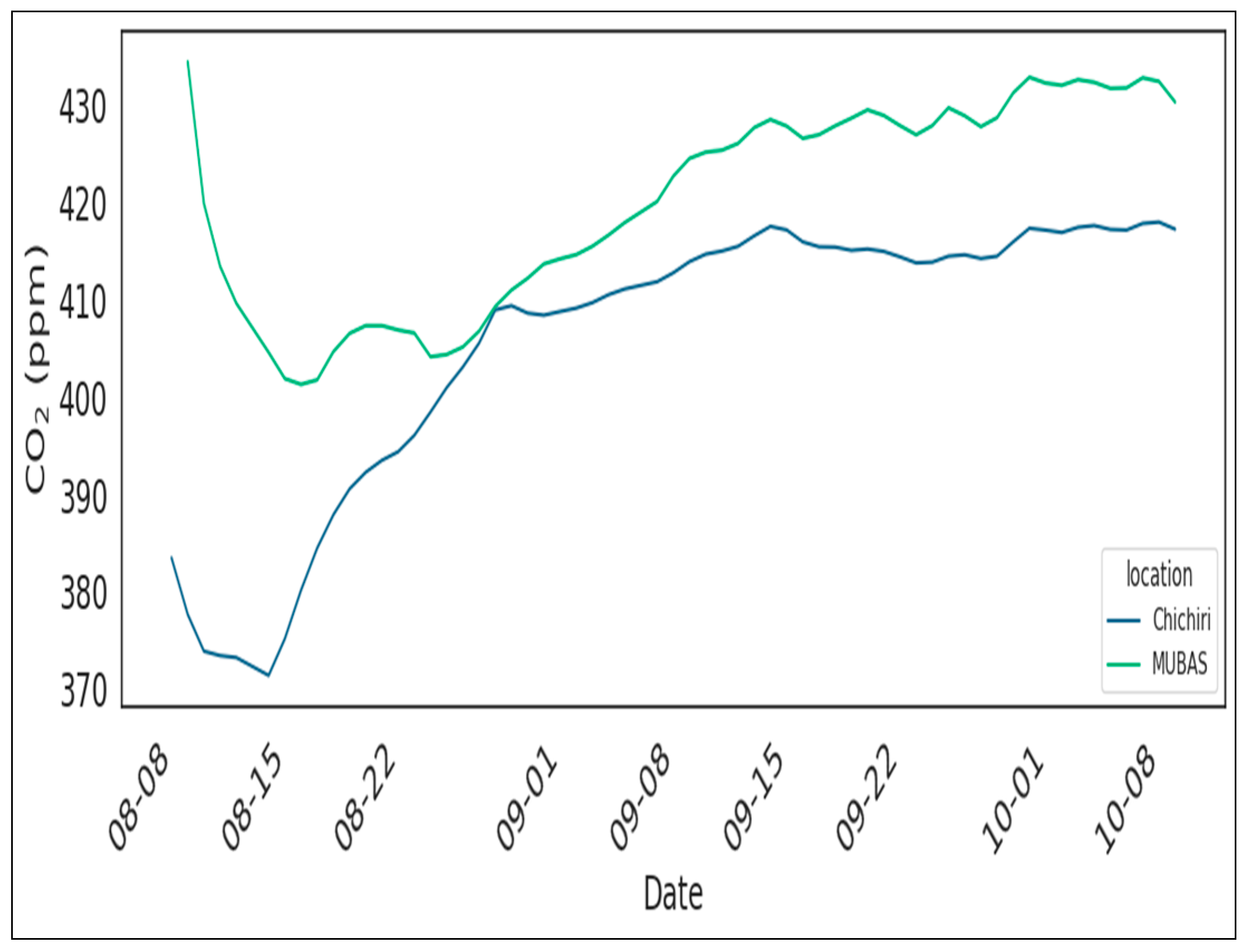
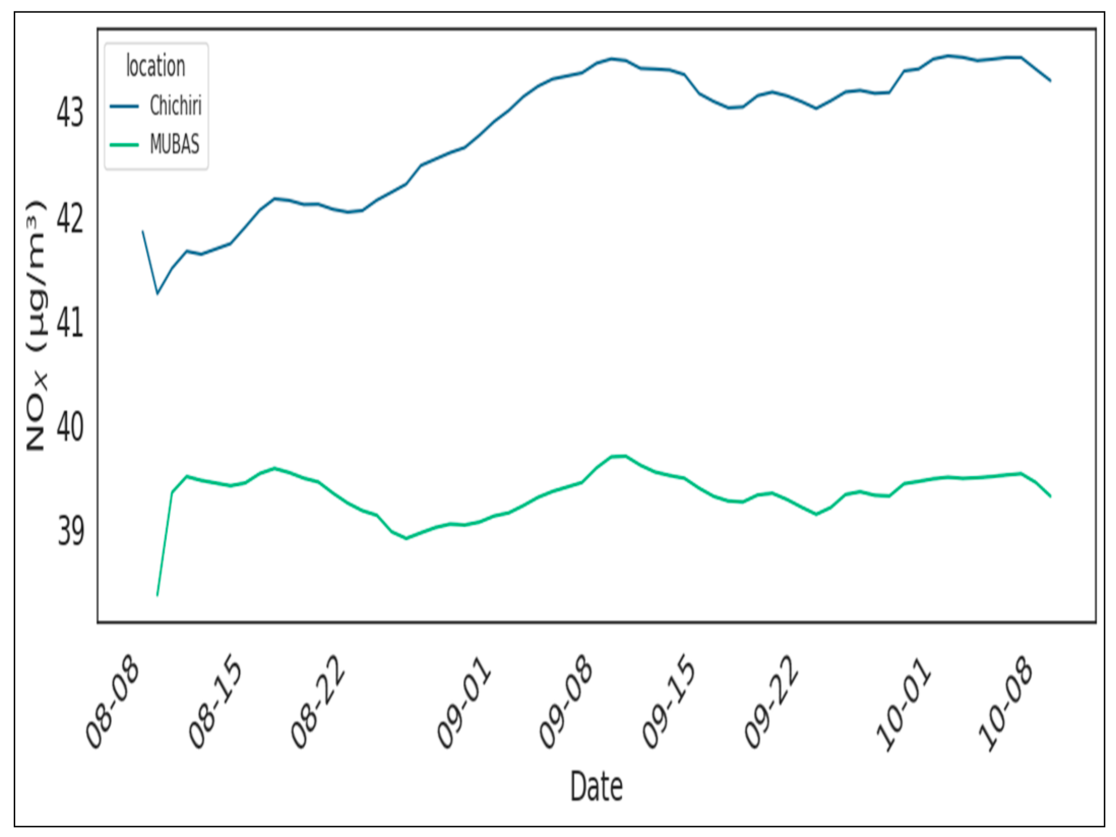
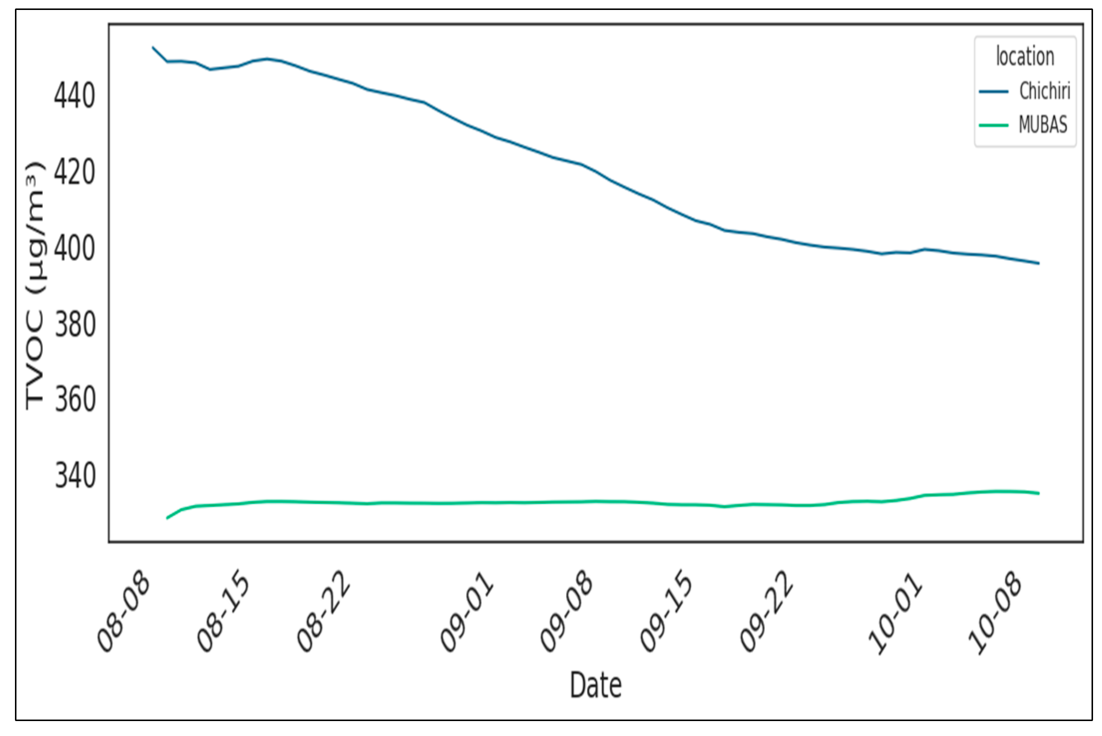
Figure 10, Figure 11 and Figure 12 show the rolling averages for ${\mathrm{C}\mathrm{O}}_2$, TVOC and ${\mathrm{N}\mathrm{O}}_{\mathrm{x}}$, respectively. A surge in ${\mathrm{C}\mathrm{O}}_2$ concentrations around MUBAS may be linked to vehicular emissions, as schools were also in session during this time (2024-2025 MUBAS academic calendar, (https://www.mubas.ac.mw/news/press-release-opening-arrangements-for-2024-2025-academic-year-11-01-2025, accessed on 20 December 2025). TVOC index values did not exceed the scaled threshold of 50,000, indicating partial reduction in outdoor chemical sources or temperature-driven volatilization.

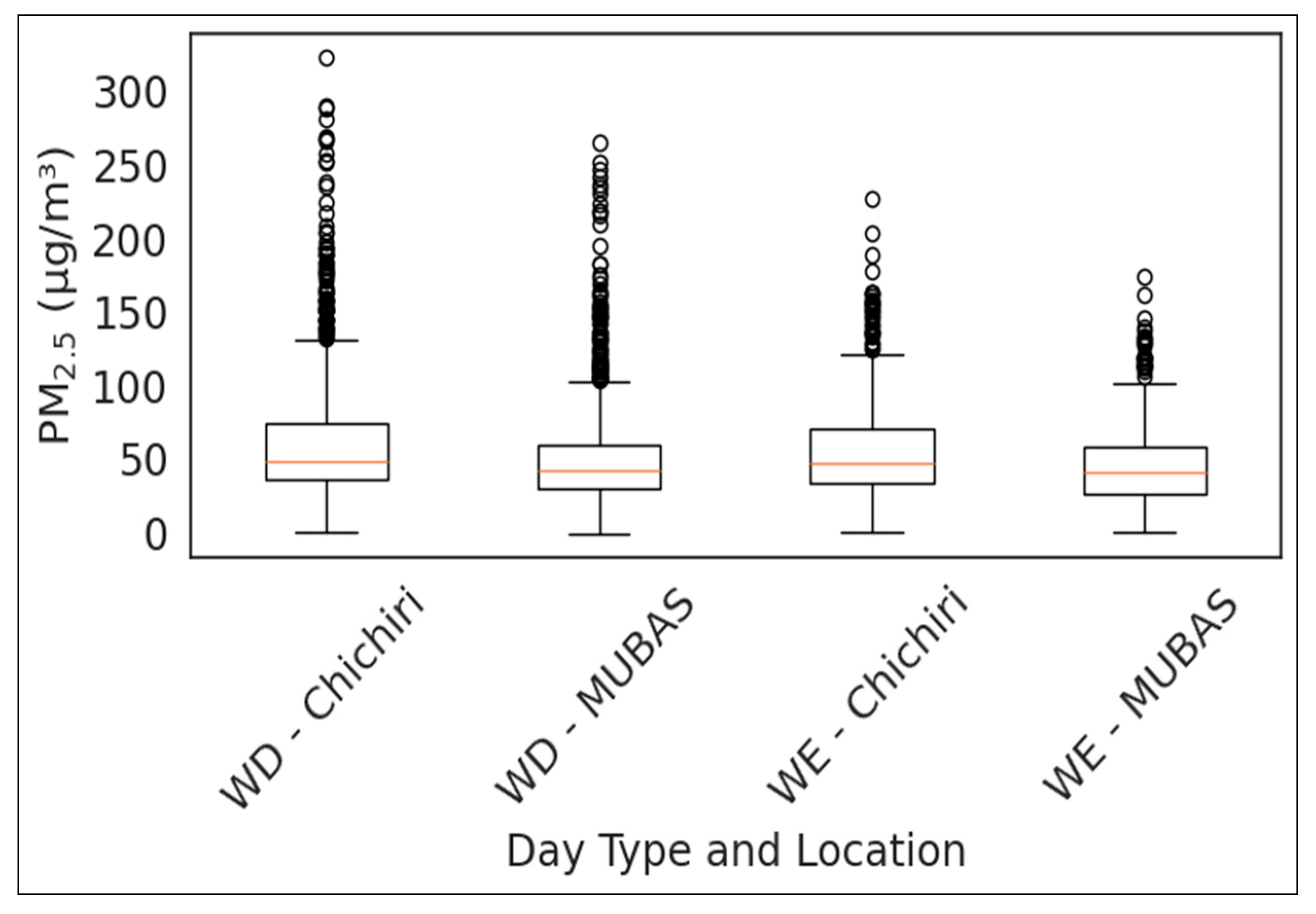
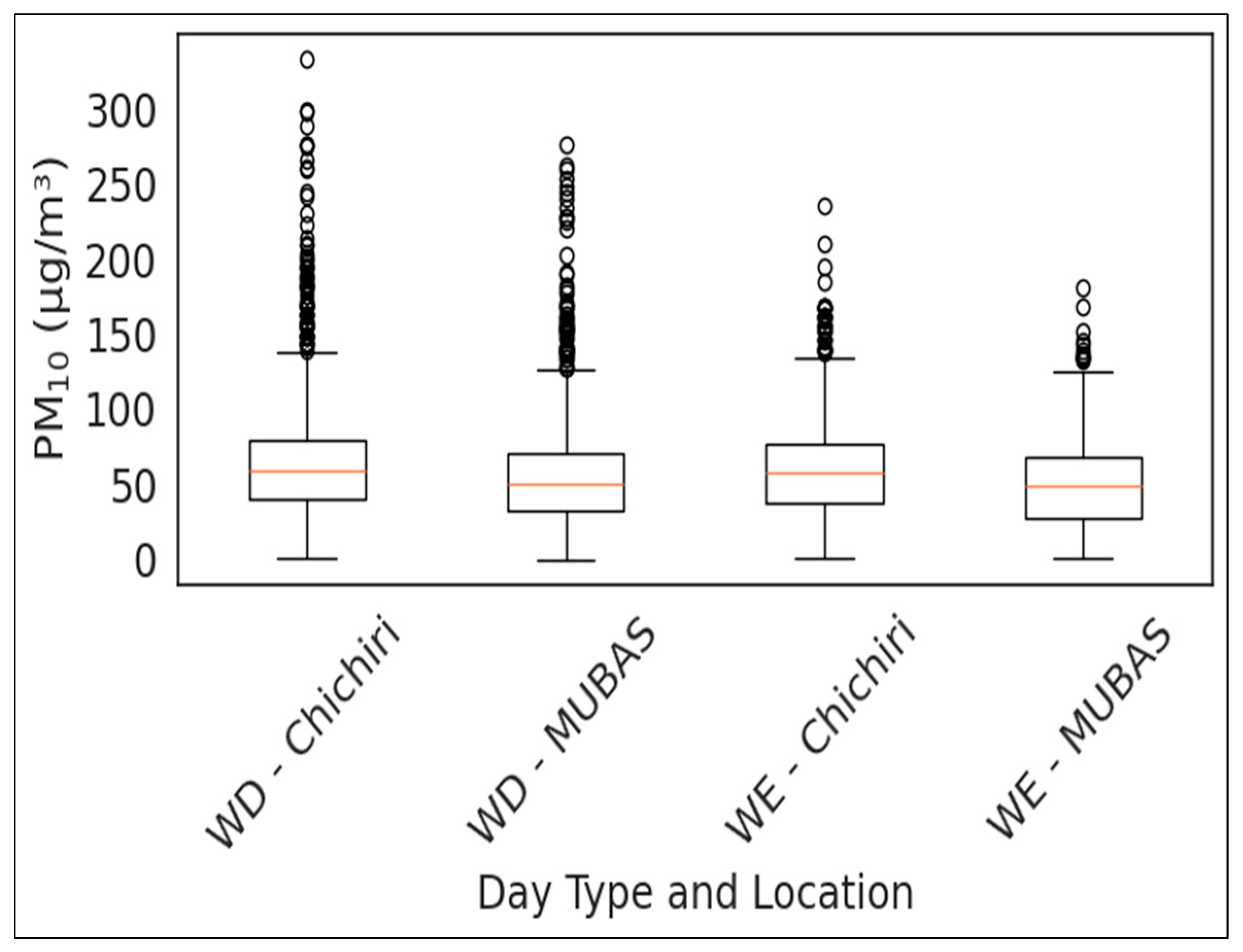
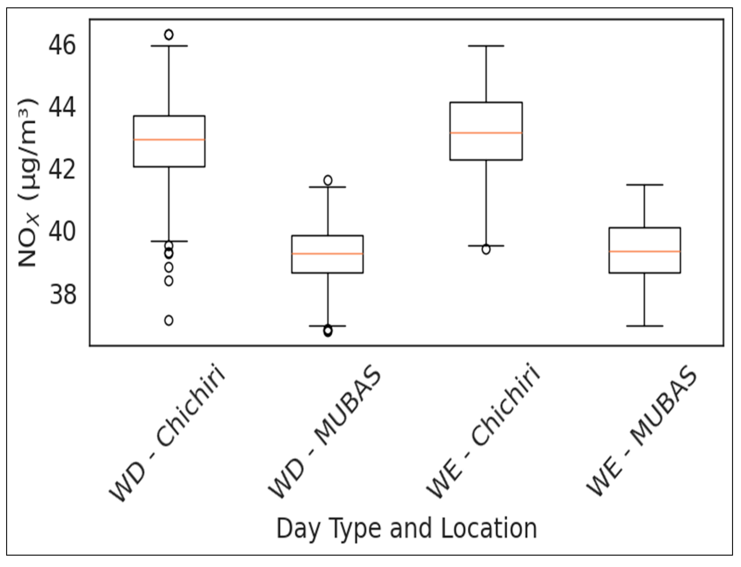
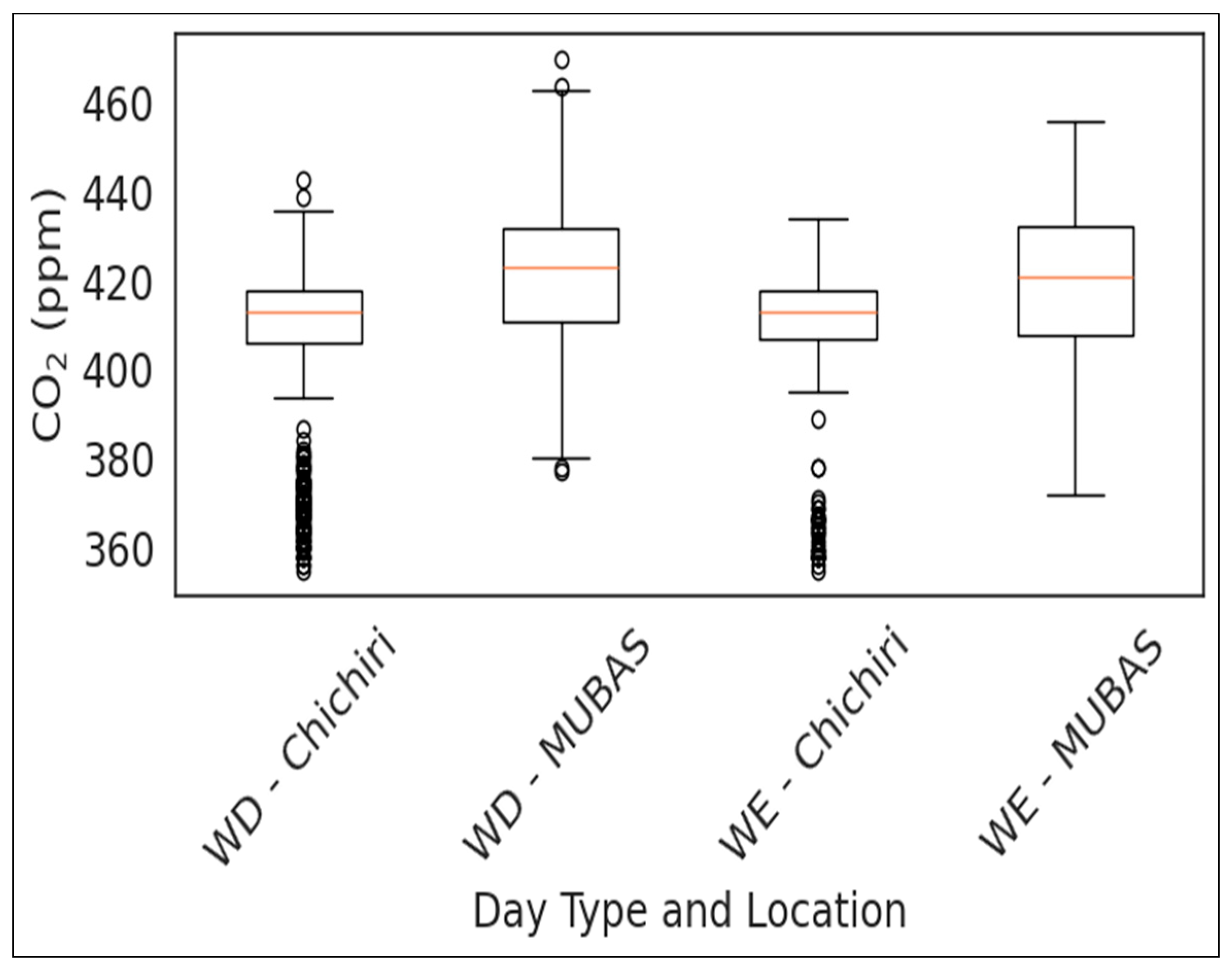
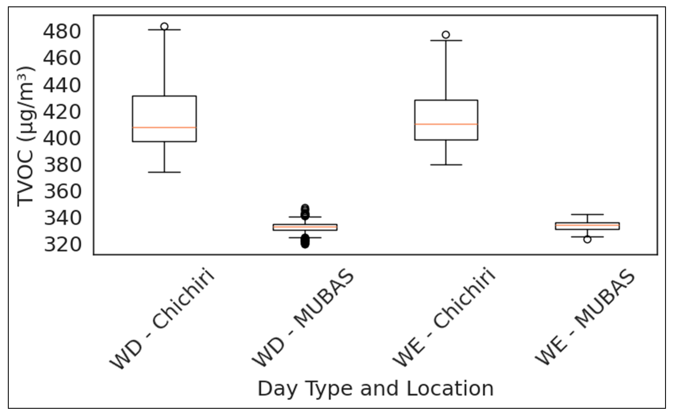
From Figure 13, Chichiri shows a broader interquartile range and outliers are an indication of greater variability and episodic pollution events likely tied to weekday (WD) traffic and combustion activities. Similarly, from Figure 14, weekday ${\mathrm{P}\mathrm{M}}_{10}$ levels exceed weekend (WE) values at both sites, with Chichiri again showing more dispersion and extreme values. ${\mathrm{C}\mathrm{O}}_2$ ${\mathrm{N}\mathrm{O}}_{\mathrm{x}}$ and TVOC concentrations are consistently higher on weekdays, especially at Chichiri, indicating increasing emission sources around this area (Figure 15, Figure 16 and Figure 17). Weekend levels are lower and more stable, certainly reflecting reduced human activity.

3.2. Exceedance Detection and AQI Classification

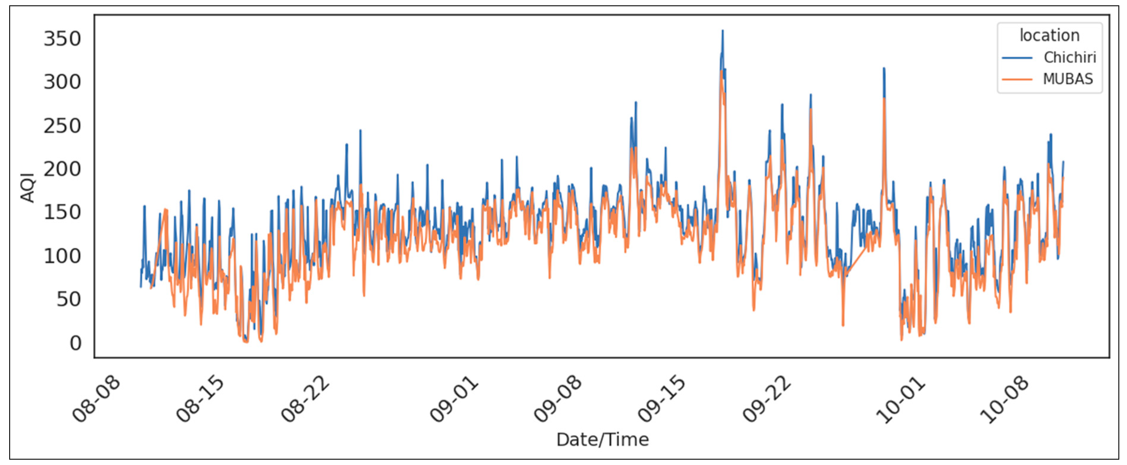
The AQI category distribution shows that most observations fall within “unhealthy for sensitive groups” and “unhealthy”, with Chichiri contributing disproportionately to more severe categories (

Table 4. AQI category distribution.

Location	Good	Hazardous	Moderate	Unhealthy	Unhealthy for Sensitive	Very Unhealthy
Chichiri	71	10	299	510	536	58
MUBAS	117	2	369	374	530	28

). MUBAS remains mostly within “moderate to unhealthy’ for sensitive groups. These fluctuations reflect the combined influence of ${\mathrm{P}\mathrm{M}}_{2.5}$, ${\mathrm{P}\mathrm{M}}_{10}$ and ${\mathrm{N}\mathrm{O}}_{\mathrm{x}}$, and align with the exceedance and category distribution patterns discussed earlier, and reinforce Chichiri’s classification as a high-risk site. Pollutant exceedance counts further validate this pattern (

Table 5. Pollutant exceedance counts.

Location	${\mathbf{P}\mathbf{M}}_{2.5}$_Exceed	${\mathbf{P}\mathbf{M}}_{10}$_Exceed	${\mathbf{N}\mathbf{O}}_{\mathbf{x}}$_Exceed	${\mathbf{C}\mathbf{O}}_2$_Exceed	TVOC_Exceed
Chichiri	1299	951	951	0	0
MUBAS	1130	712	317	0	0

). Chichiri recorded significantly more exceedances for ${\mathrm{P}\mathrm{M}}_{2.5}$ and ${\mathrm{P}\mathrm{M}}_{10}$, consistent with its elevated daily and hourly concentrations. MUBAS showed slightly more ${\mathrm{N}\mathrm{O}}_{\mathrm{x}}$ exceedance, possibly due to localized traffic. ${\mathrm{C}\mathrm{O}}_2$ and TVOC exceedance were rare, suggesting that while outdoor conformity may be compromised, outdoor acute health risks are primarily driven by particulate pollution. The AQI peaks coincide with the periods of elevated particulate matter and ${\mathrm{N}\mathrm{O}}_{\mathrm{x}}$ levels, reinforcing the role of traffic and combustion sources. The exposure to AQI $>$ 150 poses health risks, especially for vulnerable populations. The episodic nature of spikes suggests that targeted interventions during peak hours or seasons could be effective (Figure 18).

3.3. Correlation Analysis for Source Inference

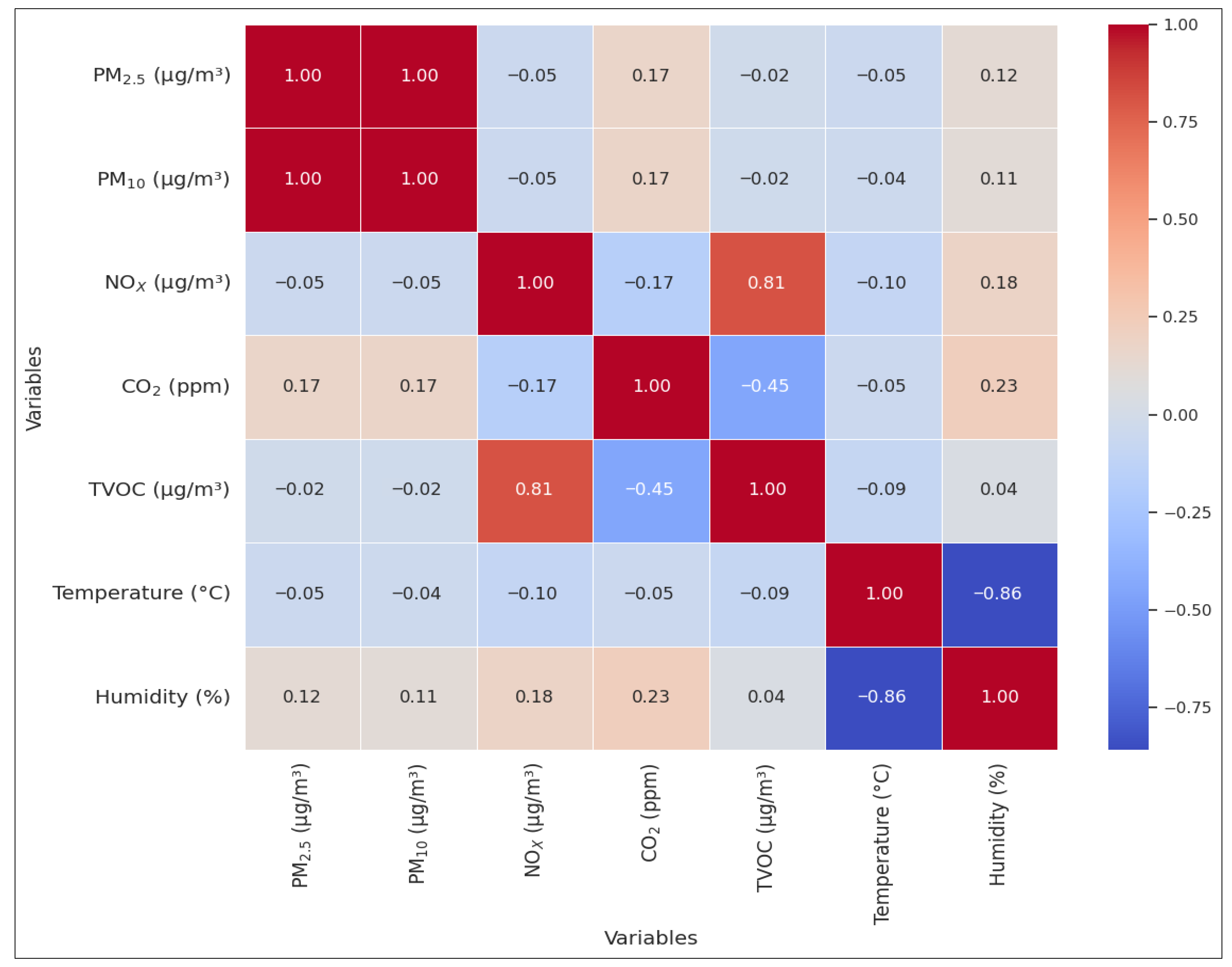
Figure 19 reveals strong inter-dependencies among pollutants and their sensitivity to meteorological conditions. The perfect correlation between ${\mathrm{P}\mathrm{M}}_{2.5}$ and ${\mathrm{P}\mathrm{M}}_{10}$ confirms their co-emission from either combustion or dust sources and validates the use of either of them as a proxy for particulate pollution. The strong negative correlations with temperature suggest that cooler conditions may suppress dispersion or coincide with increased emissions. Conversely, humidity appears to enhance particulate concentrations, possibly through hygroscopic growth or reduced atmospheric mixing. These relationships support the regression findings, where temperature and ${\mathrm{N}\mathrm{O}}_{\mathrm{x}}$ emerged as significant AQI predictors. It is therefore suggested that meteorological variables should be integrated into forecasting models and mitigation planning, especially during cooler, humid periods when pollution episodes intensify.

3.4. Multiple Linear Regression for AQI Prediction

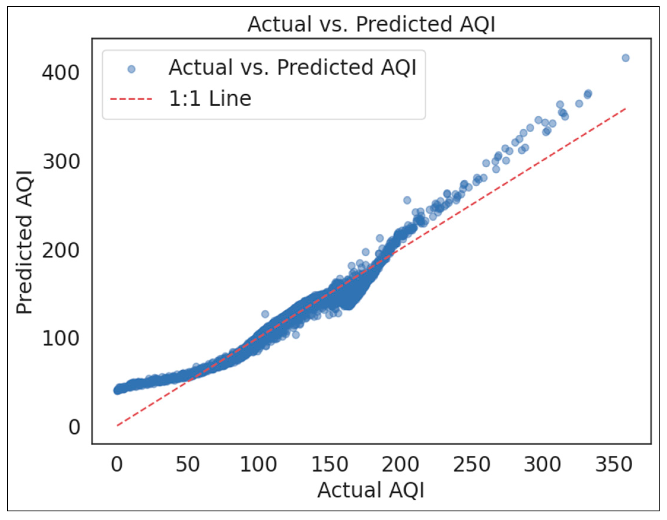
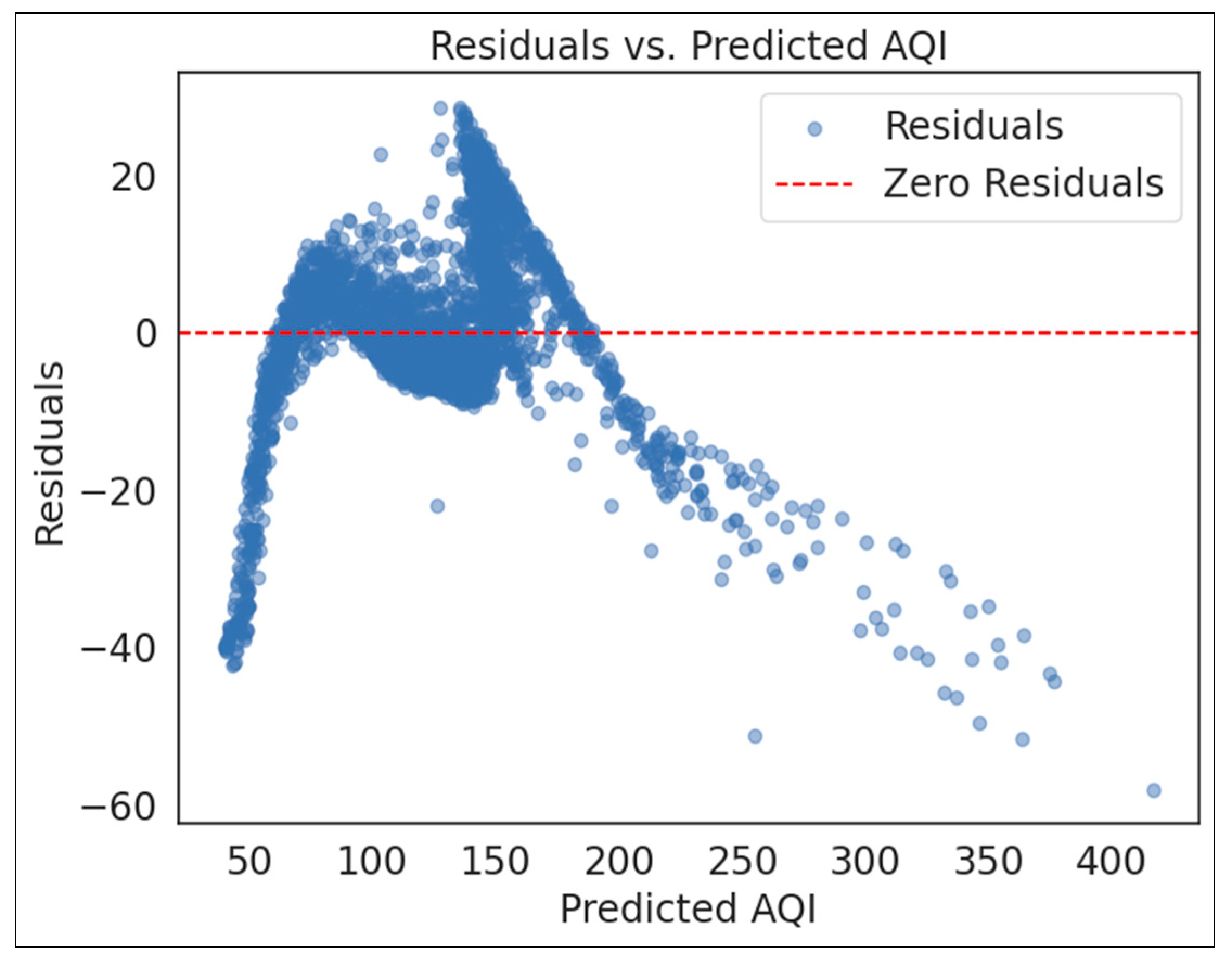
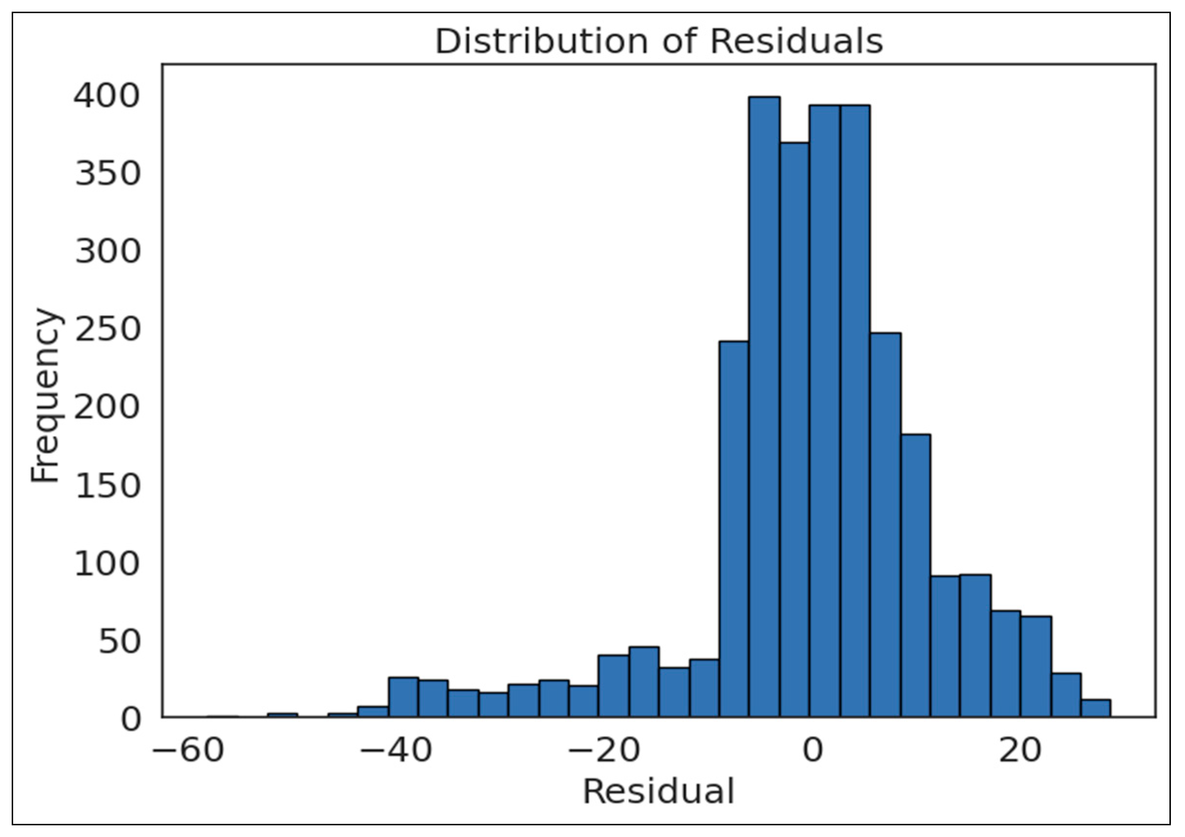
A multiple linear regression model predicted composite AQI using pollutant concentrations and meteorological variables. The model achieved a high ${\mathrm{R}}^2$ $=$ 0.938^, indicating that 93.8% of AQI variability is explained by the predictors. The ${\mathrm{R}}^2$ matched, confirming a strong fit without overfitting. Most predictors were statistically significant ($p<0.05$) (see Appendix A 

Table A1. OLS regression results.

Dep. Variable:	AQI_composite		R-squared:		0.941
Model:	OLS		Adj. R-squared:		0.941
Method:	Least Squares		F-statistic:		6527
Date:	Sun, 07 December 2025		Prob (F-statistic):		0
Time:	23:10:14		Log-Likelihood:		−5724
No. Observations	1484		AIC:		1.146 × 104
Df Residual:	1476		BIC:		1.151 × 104
Df Model:	7
Covariance Type:	nonrobust
	coeff	Std err	t	P$>$|t|	[0.025	0.975]
Const	191.9004	18.969	10.116	0.000	154.691	229.110
PM2.5 (μg/m3)	−3.1299	0.090	−24.733	0.000	−3.307	−2.953
PM10 (μg/m3)	4.1036	0.088	46.446	0.000	3.930	4.277
toNOX (μg/m3)	0.3016	0.279	1.082	0.279	−0.245	0.848
CO2 (ppm)	−0.1585	0.025	−6.257	0.000	−0.208	−0.109
TVOC (μg/m3)	0.1851	0.022	−8.243	0.000	−0.229	−0.141
Temperature (°C)	0.3249	0.131	−2.484	0.013	−0.582	−0.068
Humidity (%)	−0.1285	0.034	−3.813	0.000	−0.195	−0.062
Omnibus:	147,624		Durbin-Watson:		0.619
Prob(Omnibus):	0.000		Jarque-Bear (JB):		2995.644
Skew:	−6.630		Prob(JB):		6.34 × 10−65
Kurtosis:	4.787		Cond. No.		3.78 × 1004

and

Table A2. Correlation matrix of predictor variable.

Index	PM2.5 (μg/m3)	PM10 (μg/m3)	NOX	CO2 (ppm)	TVOC	Temperature (°C)	Humidity (%)
PM2.5 (μg/m3)	1.000000	0.996264	−0.052409	0.2051485	−0.022937	−0.050233	0.119204
PM10 (μg/m3)	0.996264	1.000000	−0.051424	0.2102879	−0.024298	−0.038450	0.105225
NOX (μg/m3)	−0.052409	−0.051424	1.000000	0.27587141	0.812243	−0.095928	0.183063
CO2 (ppm)	0.170133	0.174798	−0.167765	1.000000	−0.447987	−0.048001	0.228614
TVOC (μg/m3)	−0.022937	−0.024298	0.812243	−0.5887664	1.000000	−0.088434	0.040007
Temperature (°C)	−0.050233	−0.038450	−0.095928	0.12693236	−0.088434	1.000000	−0.858560
Humidity (%)	0.119204	0.105225	0.183063	0.03964367	0.040007	−0.858560	1.000000

). Furthermore, TVOC was not significant ($p=0.381$). ${\mathrm{P}\mathrm{M}}_{10}$ had the strongest positive effect (coefficient $=0.84$), while ${\mathrm{P}\mathrm{M}}_{2.5}$ showed a negative coefficient (−0.365), possibly due to multi-collinearity, as suggested by high condition number ($1.50\times {10}^6$). ${\mathrm{N}\mathrm{O}}_{\mathrm{x}}$ and ${\mathrm{C}\mathrm{O}}_2$ contributed positively, while temperature and humidity had small negative effects, likely reflecting dispersion dynamics. Diagnostic plots (Figure 20, Figure 21 and Figure 22) show good predictive alignment but reveal non-random residuals and slight heteroscedasticity. The residuals are approximately normally distributed, supporting model validity.

3.5. Comparison with Other African Countries

Blantyre’s ${\mathrm{P}\mathrm{M}}_{2.5}$ and ${\mathrm{P}\mathrm{M}}_{10}$ levels (with ranges of n.d.–323 $\mathsf{\mu }\mathrm{g}/{\mathrm{m}}^3$ and 0.1–333 $\mathsf{\mu }\mathrm{g}/{\mathrm{m}}^3$, respectively) are comparable to urban sites in Africa (though the maximum values are higher than most African countries), but lower than extreme values reported in Egypt, Guinea and Tanzania (

Table 6. Comparison of this study with related studies within Africa.

City, Country	Site Type	Sampling Period	${\mathbf{P}\mathbf{M}}_{2.5}$ (µg/m3)	${\mathbf{P}\mathbf{M}}_{10}$ (µg/m3)	Reference
This study	Urban	2025	n.d. *–323	0.1–333
Alexandria, Egypt	Urban	2018	1368	1805	[33]
Conakry, Guinea	Urban	December 2023–March 2024	182	435	[34]
Kinshasa, DRC	Urban	2019	43.5		[35]
Dar es Salaam	Urban	2021–2022	1008	127	[36]
Harare	Urban	June 2023–May 2024	58	34	[37]
Douala, Cameroon	Urban	January–March 2012	43.4	143.3	[38]
Korhogo, Côte d’Ivoire	Urban	April–July 2016	24.1		[39]
Abidjan, Côte d’Ivoire	Urban	Multi-site	38.0	98.0	[40]
Ouagadougou, Burkina Faso	Urban	November–December 2017	66.0	171.0	[41]
Accra, Ghana	Urban	June–July 2006	49.0	73.0	[42]
Ibadan, Nigeria	Commercial	January–March 2010		122.0	[43]
Bamako, Mali	Urban	September–October 2012 & July 2013	49.0	49.0	[44]
Durban, South Africa	Urban	2019	30–55		[45]
Highveld, South Africa	Urban	2021	35–60		[46]
Cape Town, South Africa	Urban	2010–2017		45–85	[47]
South Africa cites (multisite)	Urban	1998–2022	20–50		[48]
Sub-Saharan Africa (multi-country)	Urban	2012–2022	25–80		[49]

* not detected.

). For example, Bamako in 2013 stands out with ${\mathrm{P}\mathrm{M}}_{2.5}$ at 131 $\mathsf{\mu }\mathrm{g}/{\mathrm{m}}^3$ and ${\mathrm{P}\mathrm{M}}_{10}$ at 257.4 $\mathsf{\mu }\mathrm{g}/{\mathrm{m}}^3$, indicating severe pollution episodes as compared to this study. It should be noted that regional variation reflects differences in urban density, traffic, industrial activities and meteorological conditions. Therefore, this study contributes high-resolution data to a region with limited continuous monitoring, reinforcing the need for an expanded sensor network and harmonized AQI frameworks.

4. Conclusions and Recommendation

This study presents a comprehensive analysis of ambient air quality across two urban sites in Blantyre, Malawi, using a reproducible, senser-based workflow. Hourly and daily trends revealed consistently elevated levels of ${\mathrm{P}\mathrm{M}}_{2.5}$, ${\mathrm{P}\mathrm{M}}_{10}$ and ${\mathrm{N}\mathrm{O}}_{\mathrm{x}}$, with the Chichiri site having more severe pollution episodes than MUBAS. Across the two-month period, combining the two sites of Chichiri and MUBAS, ${\mathrm{P}\mathrm{M}}_{2.5}$ ranged from n.d.–323 $\mathsf{\mu }\mathrm{g}/{\mathrm{m}}^3$ and ${\mathrm{P}\mathrm{M}}_{10}$ ranged from 0.1–333 $\mathsf{\mu }\mathrm{g}/{\mathrm{m}}^3$; CO₂ concentrations ranged between 355 and 470 ppm, remaining below the outdoor comfort threshold. Temperature ranged from 10.7 °C to 36.5 °C. Humidity ranged from 15 to 100%. ${\mathrm{N}\mathrm{O}}_{\mathrm{x}}$ concentrations ranged from 36.8 to 46.3 $\mathsf{\mu }\mathrm{g}/{\mathrm{m}}^3$, with few exceedances relative to the guidelines. TVOC index values ranged from 372 to 483.6 $\mathsf{\mu }\mathrm{g}/{\mathrm{m}}^3$ using the applied conversion factor. AQI analysis showed that more than 60% of observations at Chichiri and 55% at MUBAS fell within “Unhealthy” or “Unhealthy for Sensitivity groups”. Frequent exposure to unhealthy, high-AQI air was mostly observed during morning and evening peaks.

A multiple linear regression model achieved high predictive accuracy (${\mathrm{R}}^2$ $=$ 0.938), identifying ${\mathrm{P}\mathrm{M}}_{10}$ ($\mathsf{\beta }=1.190)$ and ${\mathrm{N}\mathrm{O}}_{\mathrm{x}}(\mathsf{\beta }=0.214)$ as dominant contributors to AQI variability, while highlighting multicollinearity challenges with ${\mathrm{P}\mathrm{M}}_{2.5}$. Comparative analysis with Sub-Saharan African studies show that Blantyre’s pollutant levels are within the regional range but still exceed WHO guidelines, underscoring the need for targeted interventions. Meteorological factors such as temperature and humidity were found to modulate pollution dispersion, reinforcing the importance of seasonal and diurnal context in air quality management. Future research could focus on source apportionment studies, the impact of specific meteorological events and the development of more advanced predictive models to better inform policy making and interventions.

References

1. Shashi, K.A. Cardiovascular Dangers of Air Pollution. J. Clin. Cardiol. Interv. 2021, 2, 1–9. Available online: https://aditum.org/images/currentissue/1618655419JCCI-Galley_Proof.pdf (accessed on 7 December 2025).
2. Sierra-Vargas, M.P.; Teran, L.M. Air pollution: Impact and prevention. Respirology 2012, 17, 1031–1038. [Google Scholar] [CrossRef]
3. Bălă, G.-P.; Râjnoveanu, R.-M.; Tudorache, E.; Motișan, R.; Oancea, C. Air pollution exposure-the (in)visible risk factor for respiratory diseases. Environ. Sci. Pollut. Res. 2021, 28, 19615–19628. [Google Scholar] [CrossRef]
4. Chen, F.; Zhang, W.; Mfarrej, M.F.B.; Saleem, M.H.; Khan, K.A.; Ma, J.; Raposo, A.; Han, H. Breathing in danger: Understanding the multifaceted impact of air pollution on health impacts. Ecotoxicol. Environ. Saf. 2024, 280, 116532. [Google Scholar] [CrossRef] [PubMed]
5. Saleh, S.; Sambakunsi, H.; Makina, D.; Chinouya, M.; Kumwenda, M.; Chirombo, J.; Semple, S.; Mortimer, K.; Rylance, J. Personal exposures to fine particulate matter and carbon monoxide in relation to cooking activities in rural Malawi. Wellcome Open Res. 2022, 7, 251. [Google Scholar] [CrossRef]
6. Nyasulu, M.; Thulu, F.G.D.; Alexander, F. An assessment of four decades atmospheric PM2.5 trends in Southern Africa using MERRA-2 reanalysis. Air Qual. Atmos. Health 2023, 16, 2063–2084. [Google Scholar] [CrossRef]
7. Mapoma, H.W.T.; Tenthani, C.; Tsakama, M.; Kosamu, I.B.M. Air quality assessment of carbon monoxide, nitrogen dioxide and sulfur dioxide levels in Blantyre, Malawi: A statistical approach to a stationary environ-mental monitoring station. Afr. J. Environ. Sci. Technol. 2014, 8, 330–343. [Google Scholar] [CrossRef]
8. Tilley, E.; Chilunga, H.; Kwangulero, J.; Schöbitz, L.; Vijay, S.; Heilgendorff, H.; Kalina, M. It is unbearable to breathe here: Air quality, open incineration, and misinformation in Blantyre, Malawi. Front. Public Health 2023, 11, 1242726. [Google Scholar] [CrossRef]
9. ALIYU, E.H. Spatial Assessment of Gaseous Pollutants (PM2.5, PM10 SO2, NO2, CO2, CO) on Air Quality Using Air Quality Index North-Eastern Nigeria. J. Adv. Sci. Optim. Res. 2025, 7, 202–214. [Google Scholar] [CrossRef]
10. Alola, A.A.; Udemba, E.N.; Iwuagwu, C.; Abdallah, I. Assessing the human development aspects of CO, PM2.5, PM10, NOX, and SO2 in the United States. Heliyon 2023, 9, e18072. [Google Scholar] [CrossRef]
11. Do, K.; Zhang, Y. Assessing health risks and socioeconomic disparities associated with ambient air pollution and point sources across the United States. Environ. Pollut. 2025, 375, 126311. [Google Scholar] [CrossRef]
12. Meo, S.A.; Salih, M.A.; Al-Hussain, F.; Alkhalifah, J.M.; Meo, A.S.; Akram, A. Environmental pollutants PM2.5, PM10, carbon monoxide (CO), nitrogen dioxide (NO2), sulfur dioxide (SO2), and ozone (O3) impair human cognitive functions. Eur. Rev. Med. Pharmacol. Sci. 2024, 28, 789–796. [Google Scholar] [CrossRef]
13. Cipriani, G.; Danti, S.; Carlesi, C.; Borin, G. Danger in the Air: Air Pollution and Cognitive Dysfunction. Am. J. Alzheimers Dis. Other Demen. 2018, 33, 333–341. [Google Scholar] [CrossRef] [PubMed]
14. Environmental Protection Agency. Introduction Hazardous Air Pollutants; United States Environmental Protection Agency: Washington, DC, USA, 2025. Available online: https://www.epa.gov/haps (accessed on 7 December 2025).
15. Saleh, S.; Sambakunsi, H.; Mortimer, K.; Morton, B.; Kumwenda, M.; Rylance, J.; Chinouya, M. Exploring smoke: An ethnographic study of air pollution in rural Malawi. BMJ Glob. Health 2021, 6, e004970. [Google Scholar] [CrossRef]
16. Sokhi, S.R.; Moussipoulos, N.; Baklanov, S.; Bartzis, J. Advances in air quality research—Current and emerging challenges. Atmos. Chem. Phys. 2022, 22, 4615–4703. [Google Scholar] [CrossRef]
17. Clappier, A.; Thunis, P.; Beekmann, M.; Putaud, J.P.; de Meij, A. Impact of SOx, NOx and NH3 emission reductions on PM2.5 concentrations across Europe: Hints for future measure development. Environ. Int. 2021, 156, 106699. [Google Scholar] [CrossRef] [PubMed]
18. Leslie, G.B. Health Risks from Indoor Air Pollutants: Public Alarm and Toxicological Reality. Indoor Built Environ. 2000, 9, 5–16. [Google Scholar] [CrossRef]
19. Padilla, L.E.; Peters, D.R.; Mohr, E.J.; Alvarez, R.A. Ambient Measurements of Hazardous Air Pollutants in the United States Routinely Exceed Predictions from Screening-Level Exposure Models. Environ. Sci. Technol. Lett. 2025, 12, 57–63. [Google Scholar] [CrossRef]
20. Chan, C.K.; Yao, X. Air pollution in mega cities in China. Atmos. Environ. 2008, 42, 1–42. [Google Scholar] [CrossRef]
21. Duan, H.; Yue, W.; Li, W. Reliability Assessment of PM2.5 Concentration Monitoring Data: A Case Study of China. Atmosphere 2024, 15, 1303. [Google Scholar] [CrossRef]
22. Sengani, P.D.; Chandra, R.; Agarwal, G. Ambient Air Quality Assessment through Air Quality Index and Air Quality Health Index for Eastern Coastal Region, Gandhidham, Gujarat, India. Int. J. Environ. Clim. Chang. 2024, 14, 692–707. [Google Scholar] [CrossRef]
23. Goddard, S.L.; Williams, K.R.; Robins, C.; Butterfield, D.M.; Brown, R.J.C. Concentration trends of metals in ambient air in the UK: A review. Environ. Monit. Assess. 2019, 191, 683. [Google Scholar] [CrossRef]
24. Elawa, O.; Abdel-Latif, N.M.; Galal, T.M.; Farahat, E.A. Assessment of Ambient Air Quality Level at 21 sites in cement sector, Egypt. Egypt. J. Chem. 2022, 65, 47–57. [Google Scholar] [CrossRef]
25. Mapoma, H.W.T.; Xie, X. State of Air Quality in Malawi. Sci. Res. 2013, 4, 1258–1264. [Google Scholar] [CrossRef]
26. Thulu, F.G.D.; Kaonga, C.C.; Kosamu, I.B.M.; Nyasulu, M. Assessment of PM2.5 in Blantyre City, Malawi. In Advances in Air Quality Research in Africa (ICAQ Africa 2022); Fomba, K.W., Fankam, B.C., Mellouki, A., Westervelt, D.M., Giordano, M.R., Eds.; Springer: Berlin/Heidelberg, Germany, 2024. [Google Scholar] [CrossRef]
27. Utsale, C.U.; Kaonga, C.C.; Thulu, F.G.D.; Kosamu, B.M.K.; Thomson, F.; Mawenda, U.C.; Sakugawa, H. Source Apportionment of Air Quality Parameters and Noise Levels in the Industrial Zones of Blantyre City. Air 2024, 2, 122–141. [Google Scholar] [CrossRef]
28. Thulu, F.G.D.; Kaonga, C.C.; Kosamu, I.B.M.; Nyasulu, M.; Nyirongo, R.C. Longitudinal analysis of annual PM2.5 concentration variations in Blantyre City, Malawi. Clean Air J. 2024, 34, 1–12. [Google Scholar] [CrossRef]
29. World Health Organization. Particulate matter (PM2.5 and PM10), ozone, nitrogen dioxide, sulfur dioxide and carbon monoxide. In World Health Organization Global Air Quality Guidelines; World Health Organization: Geneva, Switzerland, 2021; Available online: https://www.who.int/publications/i/item/9789240034228 (accessed on 7 December 2025).
30. Hoffmann, B.; Boogaard, H.; de Nazelle, A.; Andersen, Z.J.; Abramson, M.; Brauer, M.; Brunekreef, B.; Forastiere, F.; Huang, W.; Kan, H.; et al. WHO Air Quality Guidelines 2021–Aiming for Healthier Air for all: A Joint Statement by Medical, Public Health, Scientific Societies and Patient Representative Organizations. Int. J. Public Health 2021, 66, 1604465. [Google Scholar] [CrossRef]
31. Environmental Protection Agency. How Is the AQI Calculated? United States Environmental Protection Agency: Washington, DC, USA, 2026. Available online: https://www.epa.gov/outdoor-air-quality-data/how-aqi-calculated (accessed on 7 December 2025).
32. ORCAA. EPA Updates Particulate Pollution Standards; ORCAA Olympic Region Clean Air Agency: Olympia, WA, USA, 2026; Available online: https://www.orcaa.org/epa-updates-particulate-pollution-standards/ (accessed on 7 December 2025).
33. Zahran, A.A.; Ibrahim, M.I.; Ramadan, A.E.; Ibrahim, M.M. Air Quality Indices, Sources and Impact on Human Health of PM10 and PM2.5 in Alexandria Governorate, Egypt. J. Environ. Prot. 2018, 9, 1237–1261. [Google Scholar] [CrossRef][Green Version]
34. Fofana, M.A.; Djossou, J.; Diallo, A.; Diallo, A.M. Characterization Test of PM2.5 and PM10 Particulate Matter in the Ambient Air in Conakry City, Republic of Guinea. Open J. Air Pollut. 2025, 14, 29–40. [Google Scholar] [CrossRef]
35. McFarlane, C.; Isevulambire, P.K.; Lumbuenamo, R.S.; Ndinga, A.M.E.; Dhammapala, R.; Jin, X.; McNeill, V.F.; Malings, C.; Subramanian, R.; Westervelt, D.M. First Measurements of Ambient PM2.5 in Kinshasa, Democratic Republic of Congo and Brazzaville, Republic of Congo Using Field-calibrated Low-cost Sensors. Aerosol Air Qual. Res. 2021, 21, 200619. [Google Scholar] [CrossRef]
36. Manyele, A.; Mkiramweni, M.; Senyagwa, J.; Osano, P.; Opiyo, R.; Nzuve, L. Trends of particulate matter PM2.5 and PM10 concentrations in Dar es Salaam City between 2021 and 2022. Clean Air J. 2025, 35, 1–11. [Google Scholar] [CrossRef]
37. Dangare, T.; Matandirotya, N.R.; Handizvihwe, G.; Mathe, P.; Mushore, T.D.; Matandirotya, E.; Mashonjowa, E. An assessment of ambient air quality in a densely populated urban settlement of Harare, Zimbabwe. Clean Air J. 2025, 35, 1–12. [Google Scholar] [CrossRef]
38. Ngangmo, Y.C.; Adiang, C.M. Assessment of particulate matter (PM10, PM5, PM2.5, and PM1) concentrations at significant intersections in Douala-Cameroon city using low-cost sensors. Arab. J. Geosci. 2025, 18, 94. [Google Scholar] [CrossRef]
39. Gnamien, S.; Yoboué, V.; Liousse, C.; Ossohou, M.; Keita, S.; Bahino, J.; Siélé, S.; Diaby, L. Particulate Pollution in Korhogo and Abidjan (Cote d’ivoire) during the Dry season. Aerosol Air Qual. Res. 2021, 21, 200201. [Google Scholar] [CrossRef]
40. Gnamien, S.; Liousse, C.; Keita, S.; Kumar, R.; Yoboué, V. High-Resolution Modeling of Air Quality in Abidjan (Côte d’Ivoire) Using a New Urban-Scale Inventory. Atmosphere 2024, 15, 758. [Google Scholar] [CrossRef]
41. Boman, J.; Lindén, J.; Thorsson, S.; Holmer, B.; Eliasson, I. A tentative study of urban and suburban fine particles (PM2.5) collected in Ouagadougou, Burkina Faso. X-Ray Spectrom. 2009, 38, 354–362. [Google Scholar] [CrossRef]
42. Arku, R.E.; Vallarino, J.; Dionisio, K.L.; Willis, R.; Choi, H.; Wilson, J.G.; Hemphill, C.; Agyei-Mensah, S.; Spengler, J.D.; Ezzati, M. Characterizing air pollution in two low-income neighborhoods in Accra, Ghana. Sci. Total Environ. 2008, 402, 217–231. [Google Scholar] [CrossRef] [PubMed]
43. Ana, G.; Odeshi, T.A.; Sridhar, M.K.C.; Ige, M.O. Outdoor respirable particulate matter and the lung function status of residents of selected communities in Ibadan, Nigeria. Perspect. Public Health 2014, 134, 169–175. [Google Scholar] [CrossRef]
44. Garrison, V.H.; Majewski, M.S.; Konde, L.; Wolf, R.E.; Otto, R.D.; Tsuneoka, Y. Inhalable desert dust, urban emissions, and potentially biotoxic metals in urban Saharan-Sahelian air. Sci. Total Environ. 2014, 500–501, 383–394. [Google Scholar] [CrossRef] [PubMed]
45. Buthelezi, S.A.; Kapwata, T.; Wernecke, B.; Webster, C.; Mathee, A.; Wright, C.Y. Household Fuel Use for Heating and Cooking and Respiratory Health in a Low-Income, South African Coastal Community. Int. J. Environ. Res. Public Health 2019, 16, 550. [Google Scholar] [CrossRef] [PubMed]
46. Moletsane, S.D.; Lindeque, F.; Language, B.C.; Nkosi, N.; Adesina, J.A.; Burger, R.P.; Mkhatshwa, G.; Piketh, S.J. Intra-urban variability of PM2.5 in a dense, low-income settlement on the South African Highveld. Clean Air J. 2021, 31, 1–9. Available online: https://scielo.org.za/scielo.php?script=sci_arttext&pid=S2410-972x2021000100001 (accessed on 7 December 2025). [CrossRef]
47. Arowosegbe, O.O.; Röösli, M.; Adebayo-Ojo, T.C.; Dalvie, M.A.; de Hoogh, K. Spatial and Temporal Variations in PM10 Concentrations between 2010–2017 in South Africa. Int. J. Environ. Res. Public Health 2021, 18, 13348. [Google Scholar] [CrossRef]
48. Kabanda, H.T. Investigating PM2.5 pollution patterns in South Africa using space-time analysis. AIMS Environ. Sci. 2024, 11, 426–443. [Google Scholar] [CrossRef]
49. Awokola, B.; Okello, G.; Johnson, O.; Dobson, R.; Ouédraogo, A.R.; Dibba, B.; Ngahane, M.; Ndukwu, C.; Agunwa, C.; Marangu, D.; et al. Longitudinal Ambient PM2.5 Measurement at Fifteen Locations in Eight Sub-Saharan African Countries Using Low-Cost Sensors. Atmosphere 2022, 13, 1593. [Google Scholar] [CrossRef]
Figure 1. Map of the study area.
Air 04 00008 g001
Figure 2. Setting up an air quality monitor at one of the sites.
Air 04 00008 g002
Figure 3. P M 2.5 diurnal profiles.
Air 04 00008 g003
Figure 4. P M 10 diurnal profiles.
Air 04 00008 g004
Figure 5. C O 2 diurnal profiles.
Air 04 00008 g005
Figure 6. N O x diurnal profiles.
Air 04 00008 g006
Figure 7. TVOC diurnal profiles.
Air 04 00008 g007
Figure 8. P M 2.5 daily average profile.
Air 04 00008 g008
Figure 9. P M 10 daily average profile.
Air 04 00008 g009
Figure 10. C O 2 daily average profile.
Air 04 00008 g010
Figure 11. TVOC daily average profile.
Air 04 00008 g011
Figure 12. N O x daily average profile.
Air 04 00008 g012
Figure 13. P M 2.5 weekday vs. weekend.
Air 04 00008 g013
Figure 14. P M 10 weekday vs. weekend.
Air 04 00008 g014
Figure 15. N O x weekday vs. weekend.
Air 04 00008 g015
Figure 16. C O 2 weekday vs. weekend.
Air 04 00008 g016
Figure 17. TVOC weekday vs. weekend.
Air 04 00008 g017
Figure 18. Composite AQI over time.
Air 04 00008 g018
Figure 19. Correlation matrix of pollutants vs. meteorological variables.
Air 04 00008 g019
Figure 20. Predicted AQI vs. actual.
Air 04 00008 g020
Figure 21. Residuals vs. predicted AQI.
Air 04 00008 g021
Figure 22. Distribution of residuals.
Air 04 00008 g022