An Exponential Correction to Ramanujan’s Second Formula for Ellipse Perimeter Computation

Abstract

The exact perimeter of an ellipse involves the complete elliptic integral of the second kind, which lacks a closed-form expression in elementary functions. As a result, analytical approximations have been proposed for applications requiring fast and accurate evaluation of elliptical geometries. In this study, we present a new ultra-accurate and compact closed-form approximation for the ellipse perimeter based on an exponential correction applied to Ramanujan’s second formula. The proposed expression preserves simplicity—using only three exponential functions and six constants—while achieving a maximum relative error of approximately 0.57 ppm observed over the tested grids covering the full eccentricity range. This represents a significant accuracy improvement over classical and modern approximations while maintaining a single-line analytical form with low computational cost. Due to its robustness, quasi-exact behavior at both circular and highly eccentric limits, and its suitability for numerical algorithms and embedded implementations, the proposed approximation is particularly useful in engineering computations involving elliptical boundaries.

1. Introduction

The computation of the perimeter of an ellipse is a classical problem in mathematics that has attracted attention for centuries. Unlike the circumference of a circle, which is solved by a simple closed-form expression as $P=2\pi r$, the perimeter of an ellipse with semi-axes a and b cannot be expressed as an elementary function. Instead, the exact solution involves the complete elliptic integral of the second kind. Although this expression is mathematically exact, it is computationally more expensive than a compact closed-form expression. Specifically, in practical applications this computational cost becomes important when the calculation has to be performed repeatedly, sometimes thousands of times, and a “faster formula” is evidently more convenient. For this reason, numerous analytical approximations have been proposed throughout the history of mathematics, seeking a balance between simplicity and accuracy. The challenge lies in designing compact closed-form expressions that remain highly accurate over the full range of ellipse eccentricities. In this paper, we address this challenge by proposing our exponential correction to the well known Ramanujan’s second formula.

Some current practical applications in engineering and numerical contexts where the computation of the ellipse perimeter is required are the following: In electromagnetic engineering, explicit perimeter formulas are used in the design and miniaturization of elliptical microstrip patch antennas [1]. In vibration-assisted machining, the perimeter of an elliptical tool trajectory is used to relate the cutting speed, the duty cycle, and the efficiency of the process [2]. In composite materials engineering, the perimeter of the ellipse appears in the homogenization of the multi-physical properties of fibers with non-circular cross sections, commonly evaluated using Ramanujan-type approximations [3]. Thermal modeling based on the finite element method also requires accurate estimates of the perimeter of ellipses when anatomical segments are approximated by elliptical geometries [4]. Overall, the balance of simplicity, stability, and sub-ppm accuracy makes the proposed approximation in this paper attractive for practical engineering and technological computations.

The remainder of this paper is organized as follows. Section 2 reviews the historical development of analytical approximations for the perimeter of the ellipse. Section 3 describes the methodology used to derive the proposed exponential corrections to Ramanujan’s second approximation. Section 4 presents numerical experiments and comparative error analyzes with classical and modern formulas. Section 5 discusses the results and highlights the advantages of the proposed approach, and finally Section 6 summarizes the main conclusions.

2. Historical Overview and Related Work

The exact computation of the perimeter of an ellipse has been a classical problem in mathematics since antiquity. Unlike the circumference of a circle, which admits a closed-form expression $P=2\pi r$, the ellipse with the major semi-axis a and the minor semi-axis b$(a\ge b)$ does not have a simple algebraic expression for its perimeter. Instead, the exact formula involves the complete elliptic integral of the second kind, $E\left(e\right)$, where e is the eccentricity, i.e.,

$$P_{exact}=4aE\left(e\right),\mathrm{and}E\left(e\right)={\int }_0^{\pi /2}\sqrt{1-e^2{sin}^2\theta }d\theta ,e=\sqrt{1-{\displaystyle \frac{b^2}{a^2}}}.$$

(1)

Because elliptic integrals resisted closed-form evaluation for centuries, mathematicians and scientists proposed numerous approximations, balancing simplicity with accuracy. We summarize seven formulas of historical and practical importance.

2.1. Arithmetic and Geometric Mean Approximations to the Ellipse Perimeter

Historically, astronomy has been the science that has motivated the study of ellipses and their perimeter. This is because the orbits of all celestial bodies are elliptical. There are two approaches to the perimeter of the ellipse based on Kepler’s ideas (1609) [5], which take as the perimeter of the ellipse that which corresponds to that of a circle whose radius is the arithmetic or geometric mean of the two radii of the ellipse. One of them is the arithmetic mean of the ellipse semi-axes, and the other corresponds to the geometric mean of these semi-axes [6,7]:

$$P_{AM}=\pi (a+b).$$

(2)

$$P_{GM}=2\pi \sqrt{ab}.$$

(3)

Although exact for the circle ($a=b$), these formulas become increasingly inaccurate for ellipses with a large eccentricity.

2.2. Peano’s Formula

Giusseppe Peano (1889) introduced an expression to approximate the ellipse perimeter [8], which is a weighted average between geometric and arithmetic means attributed to Kepler:

$$P_{Peano}=\pi \left(3{\displaystyle \frac{a+b}{2}}-\sqrt{ab}\right).$$

(4)

This expression is a linear combination of both means (arithmetic and geometric) resulting in a more precise approximation than each of them taken individually for low eccentricities.

2.3. Euler’s Formula

Leonhard Euler (1773) improved on this by considering the quadratic mean of the semi-axes [7,9], which is also the first term of his famous series, giving the following:

$$P_{Euler}=2\pi \sqrt{\frac{a^2+b^2}{2}}.$$

(5)

This expression is significantly more accurate than Peano’s but still yields large errors for highly elongated ellipses.

2.4. Euler-Ivory’s Series Expansion

The classical expansion in infinite series of the elliptic integral proposed by Euler in 1773 [9] in terms of n is

$$AMB={\displaystyle \frac{c\pi }{2\sqrt{2}}}\left\{1-{\displaystyle \frac{1}{2·4}}{n}^2-{\displaystyle \frac{1·1·3·5}{2·4·6·8}}{n}^4-{\displaystyle \frac{1·1·3·5·7·9}{2·4·6·8·10·12}}{n}^6-\cdots \right\}$$

where $n={\displaystyle \frac{a^2-b^2}{a^2+b^2}}$ is an eccentricity measure, $c=\sqrt{a^2+b^2}$ and $AMB$ represents the quarter of the elliptical arc, measured from the vertex A (end of the major semi-axis) to vertex B (end of the minor semi-axis) passing through the midpoint M of the said arc.

To accelerate convergence, it was rewritten in terms of h by Ivory in 1825 [10], although it is also known as Gauss-Kummer series of h:

$$\begin{array}{cc}\hfill & P_{Euler-Ivory}=\pi (a+b)\sum _{n=0}^{\infty }{\left[\left({\displaystyle \genfrac{}{}{0pt}{}{\frac{1}{2}}{n}}\right)\right]}^2{h}^n=\pi (a+b)\left[1+{\displaystyle \frac{h}{4}}+{\displaystyle \frac{h^2}{64}}+{\displaystyle \frac{h^3}{256}}+\cdots \right].\hfill \end{array}$$

(6)

Here h is a kind of eccentricity that takes values from $h=0$ for the circle to $h=1$ for the completely elongated ellipse defined as

$$h={\left({\displaystyle \frac{a-b}{a+b}}\right)}^2$$

(7)

2.5. Ramanujan I

In the early 20th century, Srinivasa Ramanujan proposed remarkably accurate approximations [7,11]. His first formula ($R1$) is

$$P_{R1}=\pi [3(a+b)-\sqrt{(3a+b)(a+3b)}].$$

(8)

This compact formula remains widely cited due to its balance of simplicity and improved accuracy.

2.6. Ramanujan II

Ramanujan also proposed, in terms of h (see Equation (7)), a second even more precise expression ($R2$) [7,11]:

$$P_{R2}=\pi (a+b)\left(1+{\displaystyle \frac{3h}{10+\sqrt{4-3h}}}\right).$$

(9)

This approximation achieves errors close to $4 \times {10}^{-4}$ or less across a wide range of axis ratios.

2.7. Ramanujan-Cantrell’s Formula

Building upon Ramanujan II, Cantrell (2004) [7] introduced an additional corrective term to further reduce the error:

$$P_{Cantrell}=\pi (a+b)\left(1+{\displaystyle \frac{3h}{10+\sqrt{4-3h}}}+c{h}^{12}\right),\mathrm{where}c={\displaystyle \frac{4}{\pi }}-{\displaystyle \frac{14}{11}}.$$

(10)

This modification reduces the maximum relative error to about $1.4\times {10}^{-5}$, representing one of the best-known simple closed-form approximations.

2.8. Koshy’s Formulas for Quarter-Perimeter

More recently, Koshy (2024) proposed two formulas for the quarter-perimeter [12], denoted $Q(a,b)$. The first formula, more accurate than the second one, is of the form

$$\begin{array}{cc}\hfill Q(a,b)& \approx Q(a,b;p)={\left(a^p+b^p\right)}^{1/p},\hfill \\ \hfill & \mathrm{where}p=p(a,b;k)={\displaystyle \frac{ln\left(2\right)}{ln(\pi /2)}}+1-{(b/a)}^k,\hfill \end{array}$$

(11)

and $k=0.03214-0.0734(b/a)+0.0863{(b/a)}^2-0.0681{(b/a)}^3+0.02306{(b/a)}^4$. Finally, the perimeter can be calculated as $P_{Koshy1}\approx 4Q(a,b)$. This approach yields a maximum error close to 8.7 ppm. The second formula proposed by Koshy is:

$$Q(a,b)\approx Q(a,b;2,k)=\sqrt{a^2+b^2}+\left({\displaystyle \frac{\pi }{2}}-\sqrt{2}\right){\left({\displaystyle \frac{GM}{AM}}\right)}^k\sqrt{ab},$$

(12)

where $k=2.6071+1.2243\left({\displaystyle \frac{b}{a}}\right)-1.2673{\left({\displaystyle \frac{b}{a}}\right)}^2+0.45566{\left({\displaystyle \frac{b}{a}}\right)}^3$, $AM={\displaystyle \frac{a+b}{2}}$, and $GM=\sqrt{ab}$.

2.9. Recent Approaches

There are other recent works, like the one proposed by Moscato in [13], giving a maximum absolute relative error of 2.7 ppm. In an effort to provide the most complete overview possible, we must mention that there are some recent approaches such as a Sykora’s optimization based on Ahmadi’s proposal in [14], that achieve very low error (<1 ppm); however, we must point out that these are reported in web compilations, and we are not aware of them having been published in peer-reviewed sources.

2.10. Error Analysis for Extreme Ratios of $a/b$

To understand the behavior of classical approximation formulas historically proposed for the perimeter of the ellipse, it is instructive to analyze their limiting behavior for extreme aspect ratios $a/b$. Two limits are particularly informative:

$${\displaystyle \frac{a}{b}}\to 1\mathrm{and}{\displaystyle \frac{a}{b}}\to \infty .$$

When $a=b$, the ellipse becomes a circle and, therefore, remembering that $P_{exact}=P_{exact}(a,b)$ (see Equation (1)) denotes the exact perimeter of an ellipse,

$$P_{exact}(a,a)=2\pi a.$$

On the other hand, as $b\to 0^{+}$ with a fixed, the ellipse degenerates into a line segment of length $2a$ and its perimeter tends to

$$P_{exact}(a,b)\to 4a.$$

The limiting relative error of any approximation $P^{\ast }(a,b)$ is defined as

$$\epsilon \left(P^{\ast }\right)={\displaystyle \frac{P^{\ast }(a,b)-P_{exact}(a,b)}{P_{exact}(a,b)}}.$$

(13)

Table 1. Limiting behavior of classical and modern ellipse perimeter approximations for the two extreme cases $a/b\to 1$ and $a/b\to \infty$. The last column reports the limiting relative error in parts per million (ppm), defined as ${10}^6\epsilon$ with $P_{exact}(a,b)\to 4a$ when $a/b\to \infty$.

Method	${\displaystyle \underset{\mathit{a}/\mathit{b}\to 1}{lim}\frac{{\mathit{P}}^{\ast }}{\mathit{a}}}$	${\displaystyle \underset{\mathit{a}/\mathit{b}\to \mathit{\infty }}{lim}\frac{{\mathit{P}}^{\ast }}{\mathit{a}}}$	$|{\mathit{\epsilon }}_{\mathit{\infty }}|$ (ppm)
Geometric mean (1609)	$2\pi$	0	$\mathrm{1,000,000}$
Arithmetic mean (1609)	$2\pi$	$\pi$	$\mathrm{214,602}$
Euler (1774)	$2\pi$	$\sqrt{2}\pi$	$\mathrm{110,721}$
Peano (1889)	$2\pi$	${\displaystyle \frac{3\pi }{2}}$	$\mathrm{178,097}$
Ramanujan I (1914)	$2\pi$	$(3-\sqrt{3})\pi$	$4155.03$
Ramanujan II (1914)	$2\pi$	${\displaystyle \frac{14\pi }{11}}$	$402.337$
Cantrell (2004)	$2\pi$	4	0
R2/2exp (proposed in this work)	$2\pi (1+2.86\times {10}^{-17})$	${\displaystyle \frac{\frac{14\pi }{11}}{1-(A+C)}\approx 3.9999999992}$	$1.94\times {10}^{-4}$

summarizes the limiting behavior of the classical formulas for the two extreme ratios of $a/b$.

3. Methodology

3.1. Numerical Computation of the Exact Elliptic Integral

In this work, the reference perimeter, P, used for the error evaluation was computed numerically using the ellipsis function ellipe from the Python (3.11.12) library mpmath (1.3.0); P is the best numerical approximation to $P_{exact}$. This library implements arbitrary-precision floating-point arithmetic and provides efficient algorithms for evaluating special functions, including elliptic integrals.

In the present computations, the default working precision of the library was used, which corresponds to approximately 15 decimal digits, which is comparable to standard double-precision arithmetic. The results reported in this paper are completely reliable because they are of the order of ${10}^{-7}$, whereas the numeric precision is of the order of ${10}^{-15}$, i.e., several orders of magnitude smaller.

3.2. One-Exponential Heuristic Correction to $R2$ ($R2/1exp$)

We started by studying the relative error curve of the classical second Ramanujan formula $P_{R2}$ given in Equation (9). From now on, for all formulas, the relative error will be calculated using Equation (13), where $P_{exact}$ is replaced by P, and $P^{\ast }$ any perimeter approximation formula. Using Equation (13), the relative error of $P_{R2}$ is $\epsilon \left(P_{R2}\right)$. We have seen that $\epsilon \left(P_{R2}\right)$ expressed as a function of h, is smooth, negative, and increases in magnitude as $h\to 1$ (high eccentricity), resembling a decaying exponential in $1-h$ of the form $\Delta \epsilon =-A{e}^{-B(1-h)}$. Therefore, if we start from the hypothesis that there must exist $\Delta \epsilon$ such that $\epsilon \left(P_{R2}\right)-\Delta \epsilon =0$, then substituting $\epsilon \left(P^{\ast }\right)$ in Equation (13) by $\Delta \epsilon$ results in

$$\Delta \epsilon ={\displaystyle \frac{P_{R2}-P}{P}}.$$

(14)

if and only if

$$P={\displaystyle \frac{P_{R2}}{1+\Delta \epsilon }}.$$

(15)

By substituting $\Delta \epsilon$ with $-A{e}^{-B(1-h)}$ in Equation (15), we obtain a better approximation to P than $P_{R2}$. Therefore, we define

$${\widehat{P}}_1={\displaystyle \frac{P_{R2}}{1-A{e}^{-B(1-h)}}},$$

(16)

where P has been replaced by ${\widehat{P}}_1$.

The parameters $(A,B)$ are fitted once (and reused universally) by minimizing a uniform error criterion over a mesh (see Algorithm 1). Specifically, we minimize the maximum absolute relative error.

$$\Phi (A,B)=\underset{(a,b)\in {\mathcal{D}}_1}{max}\left|\epsilon (a,b)\right|,{\mathcal{D}}_1=\{b=1,a\in [1,100]\}.$$

(17)

We used a numerical minimax optimization procedure [15]. The minor semi-axis was fixed at $b=1$ and the major semi-axis a was varied over a dense grid of 3000 uniformly distributed values.

The optimization seeks the set of parameters that minimizes the maximum relative error over the entire range of ellipse shapes considered. This minimax criterion ensures that the approximation remains uniformly accurate across the whole domain rather than optimizing only the average error.

In this way, we obtain the following

$$A=3.62077\times {10}^{-4},B=10.826,$$

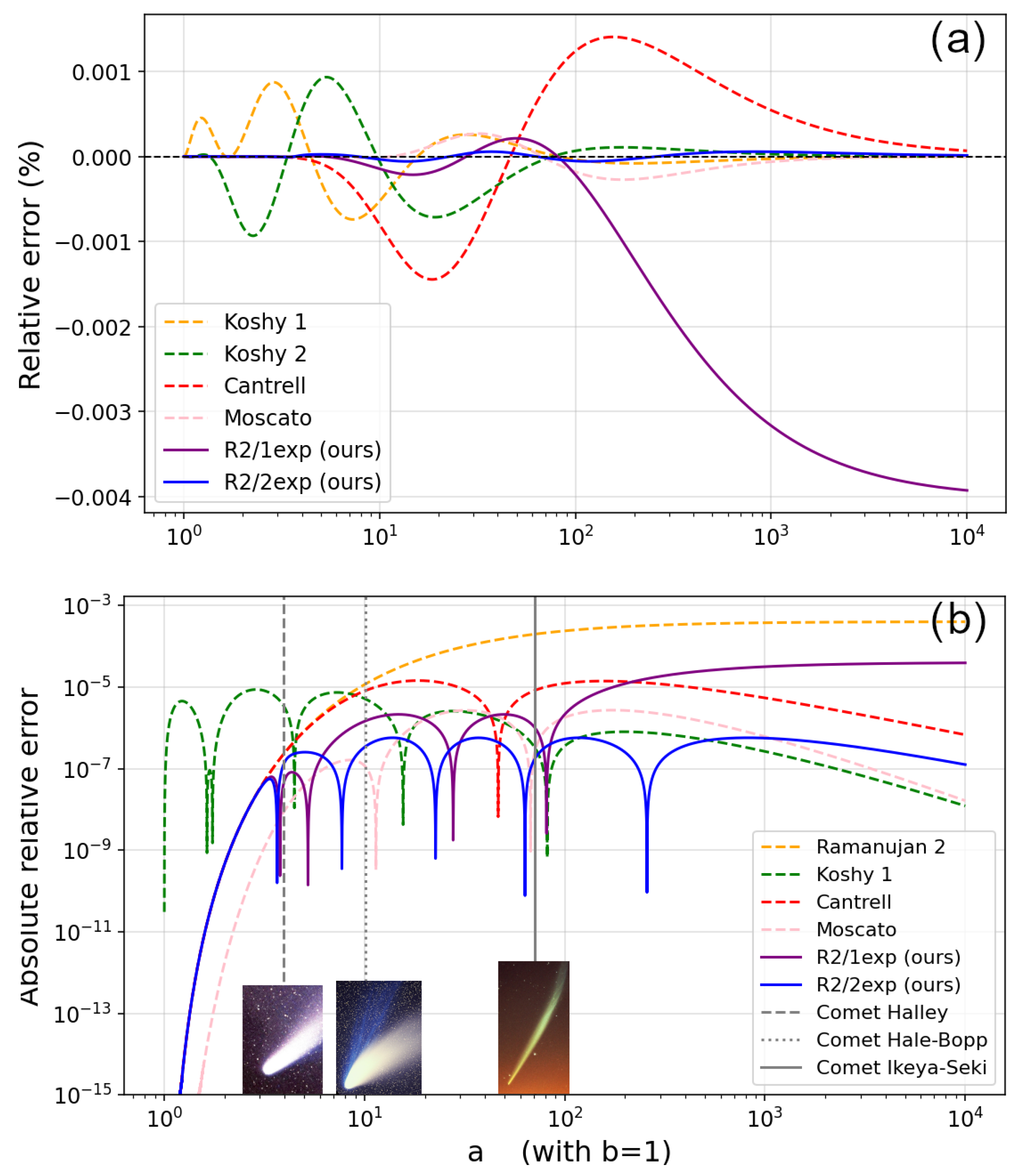
which yields a maximum relative error of about $2.14$ ppm on ${\mathcal{D}}_1$ (see Figure 1a). Equation (16) can be reliably used for $a\le 100$. An attempt was made to perform the same fitting of these constants in a wider range (from $a=1$ to $a=1000$) and the maximum relative error increased to 6 ppm, so it was decided to limit the range from a = 1 to a = 100. In an interesting fact, in this interval there are all the elliptical orbits of all known comets.

Algorithm 1 Minimax fitting of corrected Ramanujan II ellipse-perimeter approximations

Require: fixed $b>0$, interval $[a_{min},a_{max}]$, number of grid points N, model type $M\in \{1\mathrm{Exp},2\mathrm{Exp}\}$

Ensure: optimal parameters and maximum relative error

1: Construct the grid $$a_i=a_{min}+{\displaystyle \frac{i-1}{N-1}}(a_{max}-a_{min}),i=1,\dots ,N$$ 2: for $i=1,\dots ,N$ do 3:    Compute $$h_i={\left({\displaystyle \frac{a_i-b}{a_i+b}}\right)}^2,t_i=1-h_i$$ 4:    Compute the numerical approximation to the exact perimeter $$P(a_i,b)=4a_{i}E\left(1-{\left({\displaystyle \frac{b}{a_i}}\right)}^2\right)$$ 5:    Compute Ramanujan II approximation $$PR2(a_i,b)=\pi (a_i+b)\left(1+{\displaystyle \frac{3h_i}{10+\sqrt{4-3h_i}}}\right)$$ 6: end for 7: if $M=1\mathrm{Exp}$ then 8:    Define $$P^{\ast }(a,b)={\displaystyle \frac{PR2(a,b)}{1-A{e}^{-B\left(t_i\right)}}}$$ 9: else 10:  Impose $A+C=S$, set $A=S-C$ 11:  Define $$P^{\ast }(a,b)={\displaystyle \frac{PR2(a,b)}{1-\left[(S-C)e^{-B\left(t_i\right)}+C{e}^{-D\left(t_i\right)}\right]}}$$ 12: end if 13: Define minimax objective $$\Phi \left(\theta \right)=\underset{i}{max}{\displaystyle \frac{|P^{\ast }(a_i,b;\theta )-P(a_i,b)|}{P(a_i,b)}}$$ 14: Initialize a population of candidate parameters ${\theta }_j$. Being ${\theta }_j=\{A,B\}$ when $M=1\mathrm{Exp}$ or ${\theta }_j=\{C,B,D\}$ when $M=2\mathrm{Exp}$. 15: repeat 16:    for each candidate ${\theta }_j$ do 17:       Generate trial parameters by mutation and recombination 18:       Evaluate $\Phi \left({\theta }_j\right)$ 19:       Select the candidate with smaller objective value 20:    end for 21: until convergence of the population 22: Refine the best candidate using a local optimization method. Specifically Powell’s method which alternatively searches in conjugate directions. 23: Compute the maximum error and identify the worst-case grid point 24: return optimal parameters and corresponding maximum relative error

3.3. Two-Exponential Heuristic Correction to $R2$ ($R2/2exp$)

To further suppress the residual error for the very low $b/a$ ratio, i.e., $a>100$, while preserving compactness, we added a second exponential term of the same shape with parameters C and D, which are fitted with the same method as for A and B used in ${\widehat{P}}_1$. The new formula is:

$${\widehat{P}}_2^{\prime }={\displaystyle \frac{P_{R2}}{1-[A{e}^{-B(1-h)}+C{e}^{-D(1-h)}]}}.$$

(18)

We determine $(A,B,C,D)$, again by minimax fitting [15], see Algorithm 1. The fitting for $(C,D)$ was focused on high eccentricities in ${\mathcal{D}}_2=\{b=1,a\in [100,1000]\}$, while leaving the near–circular regime essentially governed by the first exponential with parameters $(A,B)$ that were also fitted. The fitting was carried out with the constraint that $A+C$ must be constant, which ensures eliminating the known error of $P_{R2}$ (Equation (9)) when ${\displaystyle \frac{a}{b}}\to \infty$, i.e., in extremely high eccentricities. This constant can be easily calculated by observing that when $h=1$ (or $a/b\to \infty$), i.e., a completely flat ellipse:

$${\displaystyle \frac{P_{R2}}{1-[A+C]}}=4a.$$

(19)

But since in that limit $P_{R2}={\displaystyle \frac{14}{11}}\pi a$, we then solve for $[A+C]$ to obtain $A+C=4.023374941\times {10}^{-4}$

The resulting new parameters for ${\widehat{P}}_2^{\prime }$ are:

$$A\approx 3.37528\times {10}^{-4},B\approx 10.29662,C\approx 6.48093\times {10}^{-5},D\approx 40.89043.$$

We have included an additional sigmoid factor $\sigma$ in order to cancel the effect of the binomial of exponential terms when $a\approx b$, i.e., in low eccentricity values:

$${\widehat{P}}_2={\displaystyle \frac{P_{R2}}{1-\sigma [A{e}^{-B(1-h)}+C{e}^{-D(1-h)}]}}.$$

(20)

in such a way that ${\widehat{P}}_2\to P_{R2}$, right there ($h<0.35$) where the second Ramanujan’s formula is highly accurate, i.e., the sigmoid function is used as a continuous step function to switch between Ramanujan II formula $P_{R2}$ and ${\widehat{P}}_2^{\prime }$. Here, $\sigma$ is the sigmoid function:

$$\sigma =\left({\displaystyle \frac{1}{1+e^{-60(h-0.35)}}}\right)$$

(21)

where $h=0.35$ is the position where the error graph of ${\widehat{P}}_2^{\prime }$ intersects with the error graph of $P_{R2}$. On the other hand, in the case of the scaling factor for the variable h, based on trial and error experiments, we have found that a value greater than or equal to 60 produces a sufficiently rapid change in the sigmoid function to commute from $P_{R2}$ to ${\widehat{P}}_2^{\prime }$ in $h=0.35$, when h increases.

The application or absence of the sigmoid function does not alter the maximum relative error reported in this paper. However, it improves the relative error, as $a/b$ tends to 1. Thus, Equation (20) attains:

• The error approaches the error in $P_{R2}$ in the range $\{b=1,a<3.42\}$,
• Maximum relative error $\approx 0.57$ ppm in the full range $\{b=1,a\in [1,\infty \left]\right\}$.

4. Numerical Evaluations

4.1. Computational Setup

All experiments used dense meshes, high–precision evaluation of P through numeric evaluation of elliptic integral $E(·)$, and reproducible code.

4.1.1. Setup for Minimax Fitting

During Minimax fitting, the objective functions are evaluated pointwise on the mesh; In Algorithm 1 $a_{min}=1$, $a_{max}=100$ for $R2/1exp$, and $a_{min}=1$, $a_{max}=1000$ for $R2/2exp$; finally $N=3000$. On the other hand, we obtain $R2/1exp$ and $R2/2exp$ as a result of the fitting process. Both Equations (16) and (20) are closed–form single–line formulas that preserve numerical stability and require only elementary operations and one exponential as in Equation (16), or two exponentials and a sigmoidal factor as in Equation (20).

4.1.2. Setup for Evaluation of the Formulas

To evaluate the accuracy of the different closed-form approximations, we designed a computational framework in Python using NumPy (2.2.6), mpmath, and Matplotlib (3.10.3). Two dense meshes with uniformly distributed dots ${10}^4$ were generated to test the methods in the following way: (1) In the h domain, setting $a=1000$ and varying $b\in [1,1000]$. (2) In the domain a, setting $b=1$ and varying $a\in$ [1.0001, 10,000]. Due to the restriction $a>b$ of Moscato’s formula, we have used $1.0001$ instead of 1.

The exact ellipse perimeter was calculated using the complete elliptic integral of the second kind in Equation (1), whose high-precision value serves as the reference benchmark. Each approximation method (Arithmetic Mean (Kepler), Euler, Ramanujan’s formula (1), Ramanujan’s formula (2), Cantrell, Koshy’s formula (1), Koshy’s formula (2), Moscato and our proposed $R2/1exp$ and $R2/2exp$) was then applied to the same mesh. For each method, we evaluated the signed and absolute value of relative error as $\epsilon \left(P^{\ast }\right)\times 100\%$ and $\left|\epsilon \right(P^{\ast }\left)\right|\times 100\%$, respectively. Finally, the maximum absolute value of all relative errors was extracted. The computational framework for testing all methods are available to anyone in [16].

4.2. Relative Error Comparison (Selected Methods)

Figure 1a shows the signed relative error for the six most accurate closed-form approximations: Cantrell, Koshy 1, Koshy 2, Moscato, $R2/1exp$ [using the sigmoid factor $\sigma$ multiplying the constant A of Equation (16)], and $R2/2exp$ (Equation (20)) as a function of a, while b remains constant and equal to 1. From $a=1$ to $a=100$, the plot highlights that while Cantrell, Koshy 1, and Koshy 2 methods achieve errors ≈$+/-0.001\%$, Moscato’s and $R2/1exp$ achieve maximum relative errors of around $+/-0.00025\%$. In contrast, $R2/2exp$ remains much closer to zero and less than $+/-0.00001\%$ across the same range. From $a=100$ to a = 10,000, the error of our first formula $R2/1exp$ increases negatively from $-0.00021\%$ to $-0.004\%$ at a = 10,000. This is explained by the fact that the fitting of the constants for this formula was made from $a=1$ to $a=100$, while in the $R2/2exp$ method, the error remains less than $0.00001\%$ throughout the interval ($a=1$ to a = 10,000). Figure 1b shows on a logarithmic scale the absolute relative error for the same techniques. As an illustrative reference, we locate the orbits of three known comets, all with $a<100$.

4.3. Summary of Maximum Errors

Table 2. Maximum relative error (% and ppm) of ellipse perimeter approximations. The Moscato’s formula requires the parameter b being equal to 1 because it contains exponents where the parameter a is isolated, this is the reason of a dash symbol in the table.

Formula	a = 1000 and $\mathit{b}\in [1,1000]$	b = 1 and $\mathit{a}\in [1.0001,100]$	b = 1 and $\mathit{a}\in [100,1000]$
A.M. Equation (2)	21.38195%/213,819.50 ppm	20.69656%/206,965.61 ppm	21.38195%/213,819.50 ppm
Euler	11.0717% /110,716.96 ppm	11.04714%/110,471.35 ppm	11.07170%/110,716.96 ppm
Ramanujan I	0.4068762%/4068.76 ppm	0.3420281%/3420.28 ppm	0.4068762%/4068.76 ppm
Ramanujan II	0.03784220%/378.42 ppm	0.0238977%/238.98 ppm	0.0378422%/378.42 ppm
Cantrell	0.001446076%/14.46 ppm	0.001446075%/14.46 ppm	0.001406936%/14.07 ppm
Koshy 2	0.0009337747%/9.34 ppm	0.0009337747%/9.34 ppm	0.0001083570%/1.08 ppm
Koshy 1	0.0008735187%/8.74 ppm	0.0008735186%/8.74 ppm	0.00008046597%/0.80 ppm
Moscato	—	0.0002697398%/2.70 ppm	0.0002721463%/2.72 ppm
R2/1exp	0.003167%/31.67 ppm	0.00021458%/2.14 ppm	0.003167%/31.67 ppm
R2/2exp	0.0000573%/0.57 ppm	0.0000573%/0.57 ppm	0.0000573%/0.57 ppm

summarizes the maximum relative errors (in % and ppm) of ten methods computed over three different ranges: ($a=1000$ and $b\in [1,1000]$), ($b=1$ and $a\in [1.0001,100]$), and ($b=1$ and $a\in [100,1000]$). As can be seen, the oldest formulas (Kepler and Euler) exhibit errors exceeding 10%. The Ramanujan’s approximations reduce the error drastically to the order of $0.1$% or less. Cantrell and Koshy achieve errors in the order of $0.001$%. On the other hand, Moscato only achieves good results, on the order of 3 ppm, when parameter b is set to 1 and parameter a is varied. In contrast, our proposed correction $R2/2exp$ further improves the maximum error to approximately $0.57$ ppm, making it the most accurate among all closed-form, single-line known methods.

Table 3. Locations in h of the maximum relative error of modern ellipse perimeter approximations.

Formula	$\mathit{h}\in [0,1]$	Absolute Maximum Relative Error (ppm)
Ramanujan I	1	4155.03
Ramanujan II	1	402.337
Cantrell	0.805747	14.4608
Koshy 2	0.469204	9.33774
Koshy 1	0.234143	8.73519
Moscato	0.977093	2.72138
R2/1exp (proposed)	1	40.27
R2/2exp (proposed)	0.7483	0.573

illustrates the positions in h of the maximum relative error of modern ellipse perimeter approximations.

Due to fine-tuning of the parameters A and C, the relative error decreases from $0.57$ ppm to $1.94\times {10}^{-4}$ ppm as the eccentricity increases, reaching the flat ellipse limit when $b/a\to 0$, or $e\to 1$, $h\to 1$.

The reported maximum relative errors correspond to the largest values observed over dense numerical grids covering the domain of interest. Although the sampling is sufficiently fine to capture the error behavior with high confidence, these values should be interpreted as empirical maxima rather than strict global bounds. A formal proof of global optimality or worst-case error bounds is beyond the scope of this work.

5. Discussion

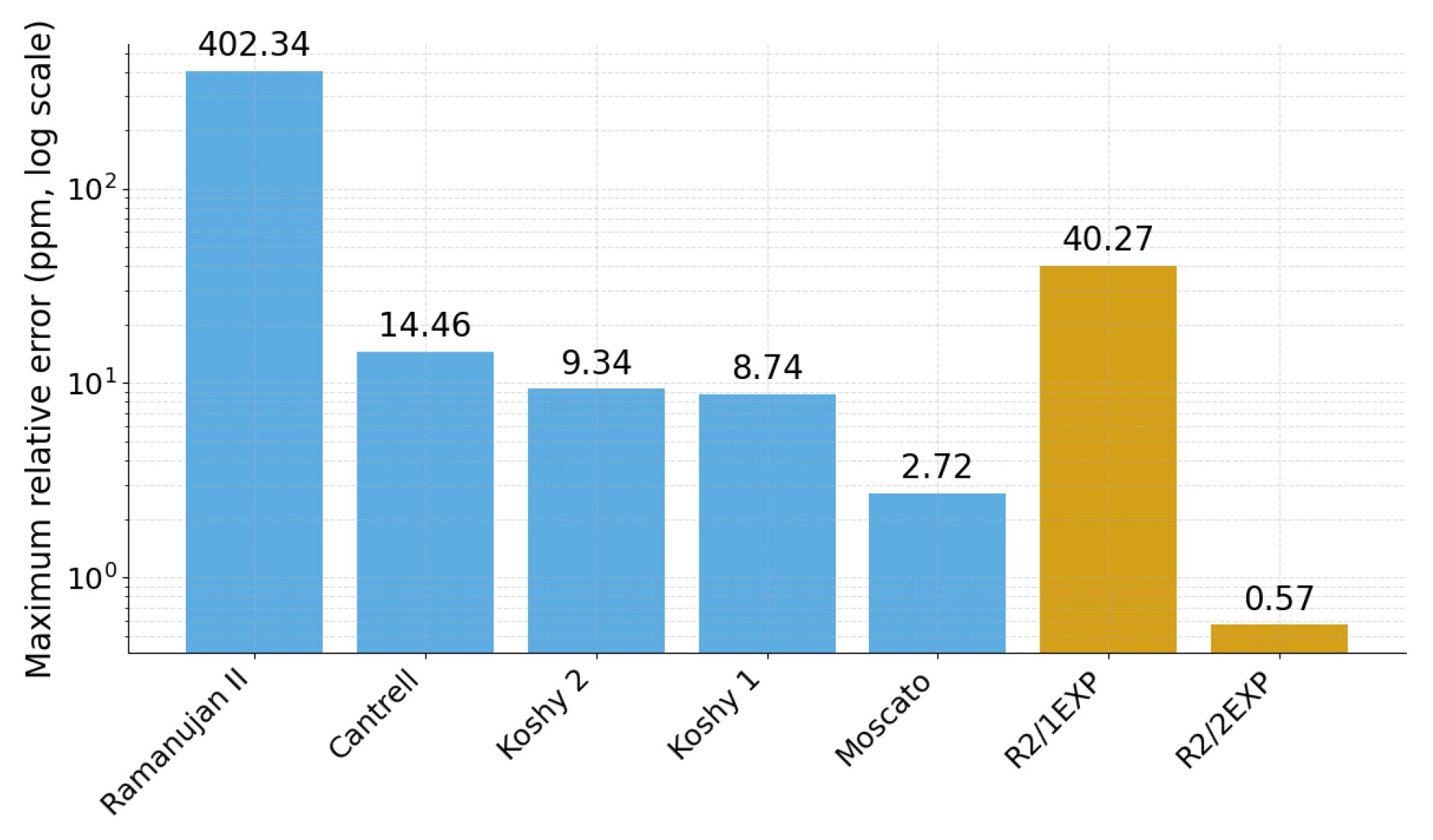
The comparative analysis of maximum relative errors provides a clear picture of the performance of classical and modern closed-form approximations for the ellipse perimeter. The results are summarized in Table 2, and the discussion below highlights both qualitative trends and quantitative comparisons. The earliest formulas, such as Kepler and Euler, offer only rough estimates: their errors grow quickly as the ellipse becomes more eccentric, with deviations exceeding 10%. Ramanujan’s contributions mark a significant leap in accuracy: both $R1$ and $R2$ drastically reduce the error, with $R2$ already achieving a maximum relative error of 378 ppm. Later refinements by Cantrell and Koshy succeeded in pushing the error to $14.46$ ppm and $8.74$ ppm, respectively. The latter reaching an accuracy of sub-10 ppm across most of the tested range. Our first exponential correction to Ramanujan’s formula $R2/1exp$ produces a remarkable result of only 2.14 ppm in the range from $a=1$ to $a=100$ while keeping $b=1$. We used this range due to its usefulness in covering the range of eccentricities of all known celestial bodies. Subsequently, with the aim of further expanding the range of eccentricities for $R2/1exp$, we again fitted from $a=1$ to $a=1000$. This time, we obtained a maximum relative error of 6 ppm and a negative growth from $a=1000$ onward. For this reason, we decided to return to the previous adjustment made from $a=1$ to 100 and which gave an error of $2.14$ ppm. In this case, we observed that the relative error as a function of h decreases negatively from $a=100$ and that this curve also resembles a negative exponential function. Therefore, we decided to add an extra exponential term; that is, we added an exponential term to the first term that already existed in $R2/1exp$. Then, we introduced the constraint $A+C=4.023374941\times {10}^{-4}$, which guarantees the cancellation of $R2$ error at $h=1$. Once this constraint was taken into account, we fitted B, C and D from $a=1$ to 1000 for $R2/2exp$.

$R2/2exp$ is a single-line expression that requires only five exponentiations. To our knowledge, this formulation achieves the lowest error observed over the tested grids, which is below $0.58$ ppm in the entire range while maintaining minimal computational overhead.

To contextualize the improvement, we compare the maximum relative error of each method with the proposed formula $R2/2exp$ as shown in Figure 2.

Finally, and as an additional piece of information we have computed Euler-Ivory expansion in Equation (6) and have seen that 148 terms of the series are required to reach a maximum relative error of 0.57 ppm in the same interval $b=1$, and $a\in [1,1000]$ that we used for our $R2/2exp$ approximation.

6. Conclusions

We summarize the main conclusions as follows:

• A compact closed-form approximation for the ellipse perimeter has been developed by introducing an exponential correction to Ramanujan’s second formula.
• We have designed a method with exceptional accuracy that simultaneously preserves minimal computational and notational overhead. Specifically, our expression is a compact closed-form and single-line formula that achieves [Equation (20)] a maximum relative error of approximately $0.57$ ppm (at $a/b=13.820656$, $e=0.997379$, $h=0.748317$) over the dense grids tested covering the full eccentricity range, i.e., $0\le h\le 1$.
• As far as we know, our method outperforms in accuracy and compactness all other approaches that are currently reported in peer reviewed publications.
• In this project, we have shown that even more refined and modern formulas of Cantrell, Koshy and Moscato, still have errors of 25, 15, and $4.7$ times larger than ours, respectively.

References

1. Sivagnanam, S.; Kailasapathi, P.; Ramesh Kumar, S. A Multi-band crescent shaped microstrip patch antenna with spiral shape ground slot for UWB applications. Int. J. Res. Eng. Appl. Manag. 2018, 4, 489–493. [Google Scholar]
2. Brehl, D.E.; Dow, T.A. Review of vibration-assisted machining. Precis. Eng. 2008, 32, 153–172. [Google Scholar] [CrossRef] [Scilit]
3. Nakka, R.; Kumar, A.P.; Harursampath, D.; Ponnusami, S.A. Influence of fibre cross-section profile on the multi-physical properties of uni-directional composites. Compos. Struct. 2023, 321, 117321. [Google Scholar] [CrossRef] [Scilit]
4. Sun, X. Development of an Improved Thermal Model of the Human Body and an Experimental Investigation of Heat Transfer from a Moving Cylinder. Ph.D. Thesis, Kansas State University, Manhattan, KS, USA, 2012. [Google Scholar]
5. Kepler, J. Astronomia Nova; G. Voegelinus: Heidelberg, Germany, 1609; Available online: https://archive.org/details/Astronomianovaa00Kepl (accessed on 21 March 2026).
6. Almkvist, G.; Berndt, B. Gauss, Landen, Ramanujan, the arithmetic–geometric mean, ellipses, π, and the Ladies Diary. Am. Math. Mon. 1988, 95, 585–608. [Google Scholar]
7. Sýkora, J. Approximations of Ellipse Perimeters and of the Complete Elliptic Integral E(x). Review of Known Formulae. Ebyte.it Stan’s Library III. 2005. Available online: http://www.ebyte.it/library/docs/math05a/EllipsePerimeterApprox05.html (accessed on 21 March 2026).
8. Kennedy, H.C. Selected Works of Giuseppe Peano; University of Toronto Press: Toronto, ON, Canada, 1973; Available online: http://www.jstor.org/stable/10.3138/j.ctt1vxmd8x (accessed on 21 March 2026).
9. Euler, L. Nova Series Infinita Maxime Convergens Perimetrum Ellipsis Exprimens. 1774. Available online: https://scholarlycommons.pacific.edu/euler-works/448 (accessed on 21 March 2026).
10. Michon, G.P. Final Answers: Perimeter of an Ellipse. 2007. Available online: https://www.numericana.com/answer/ellipse.htm (accessed on 21 March 2026).
11. Ramanujan, S. Modular equations and approximations to π. Q. J. Math. 1914, 45, 350–372. Available online: https://ramanujan.sirinudi.org/Volumes/published/ram06.pdf (accessed on 21 March 2026).
12. Koshy, K.I. Ellipse perimeter approximation: Two high accuracy formulae derived from a perimeter property. Int. J. Sci. Res. Math. Stat. Sci. 2024, 11, 1–5. [Google Scholar]
13. Moscato, P.; Ciezak, A. A new approximation for the perimeter of an ellipse. Algorithms 2024, 17, 464. [Google Scholar] [CrossRef] [Scilit]
14. Sýkora, S. Advances in Approximations of Ellipse Perimeters and of the Complete Elliptic Integral. Stan’s Library. 2007. Available online: https://www.researchgate.net/publication/331938805_Advances_in_Approximations_of_Ellipse_Perimeters_and_of_the_Complete_Elliptic_Integral (accessed on 21 March 2026).
15. Powell, M.J.D. Approximation Theory and Methods; Cambridge University Press: Cambridge, UK, 1981. [Google Scholar]
16. Ayala-Raggi, S.E. Ellipse Perimeter Approximation. GitHub Repository. 2026. Available online: https://github.com/sraggi/ellipse_perimeter_approx (accessed on 21 March 2026).
Figure 1. (a) Signed relative error comparison of ellipse perimeter approximations. The graph shows that R 2 / 1 e x p (purple) outperforms the others methods when a < 100, while R 2 / 2 e x p (blue) outperforms all methods across the entire range ( a < 10,000). (b) Absolute relative error comparison and three references of elliptical orbits of famous comets.
Appliedmath 06 00056 g001
Figure 2. Maximum relative error for all the range of eccentricities ( 0 h 1 ) of the most accurate perimeter approximations (20th and 21st centuries).
Appliedmath 06 00056 g002