Bayesian Chance-Constrained Planning Under Limited Sampling for Sectional Warping

Abstract

Sectional warping requires selecting a final operating length when only a small sample of residual cone masses can be measured. This paper proposes a Bayesian chance-constrained planning rule that combines a conjugate log-space model with fast posterior predictive simulation of the population minimum to recommend a risk-limited band length. The method provides a transparent risk parameter, efficient computation, and direct comparison with heuristic, bootstrap, distribution-free, and tail-model baselines. In an industrial-like synthetic study, the Bayesian policy reduced the mean remainder relative to a tuned sample-minimum rule while maintaining controlled shortage risk, and the results clarify why fully distribution-free guarantees are impractical under typical sampling budgets.

1. Introduction

Warp preparation in weaving converts yarn packages mounted on a creel (Spanish: fileta) into a warp beam containing hundreds or thousands of parallel ends with controlled tension, alignment, and length. Standard references distinguish direct (beam) warping from indirect (sectional) warping, in which narrow warp sections are first wound on a drum and later beamed off to the weaver’s beam [1,2,3]. Sectional warping is selected for short runs, delicate yarns, and complex repeats, and it is typically integrated with sizing and drawing-in operations in the overall weaving preparation chain [3].

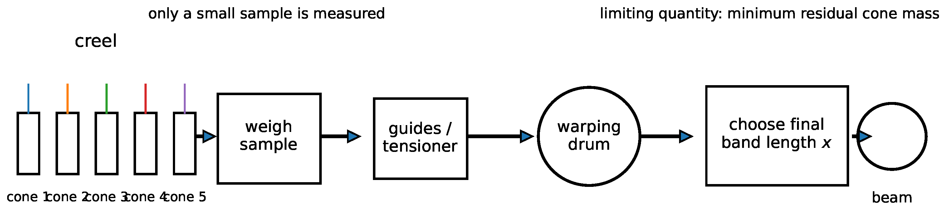
The schematic overview in Figure 1 is used to identify the cones on the creel, the yarn path through the guides and tensioning elements, the warping drum, and the final-band decision point referenced in the problem statement.

In this arrangement, the limiting quantity is the smallest residual mass among the cones feeding the last band, while the operational decision is the useful band length to be planned before winding stops.

In a sectional warper, each end is unwound from a cone, passes through guides and tensioning elements, and is wound onto the drum in successive bands. After each band, the same population of cones is partially depleted. The final band is therefore fed by cones with heterogeneous residual masses. At this stage the operator must decide a target final-band length x (m/end) that (i) uses as much of the remaining yarn as possible while (ii) avoiding an end-out event in which at least one end runs out before reaching x.

Operationally, an end-out can trigger interventions (cone changes, splices, rethreading) and create downtime. Even in well-managed plants, restarts and transient tension control consume extra length and can introduce quality risks. To reduce the probability of shortage, practitioners often adopt conservative rules (e.g., stopping early or replacing cones preemptively), which systematically leave large remainders on cones. This conservatism is exacerbated by a practical constraint: weighing all N cones at the moment of decision is usually infeasible, so only a small sample can be weighed and extrapolated.

Existing research in warp preparation has largely focused on process quality, automation, and machine dynamics (e.g., motion control and winding thickness control in sectional warpers) [4,5]. Recent work has continued to emphasize preparatory-stage performance improvement, tension regulation in warp preparation and sizing, retrofit tension-control systems in direct warp preparation, and faster yarn-break detection in warping equipment [6,7,8,9,10]. In contrast, the planning problem of selecting the final-band length under partial information about residual cone content remains largely heuristic in many production settings.

The last-band decision has a distinctive mathematical structure. Completion is governed by the smallest available length among the N ends; equivalently, it depends on the population minimum of residual cone mass. The decision can therefore be framed as a chance-constrained optimization problem [11,12] driven by an extreme order statistic [13,14]. Because the minimum is sensitive to the lower tail, small uncertainty about tail behavior can translate into large differences in “safe” band length.

We propose a Bayesian posterior predictive decision rule that translates a small set of cone weighings into a single operational length recommendation with an explicit risk parameter $\epsilon$. A conjugate model in log-space (Normal–Inverse-Gamma) supports fast updates and transparent prior elicitation from historical runs. We also include posterior predictive checks and stress tests to evaluate tail adequacy [15,16].

To keep the Introduction focused on the problem setting, the contribution summary is moved to the end of Section 6, immediately before the Conclusions.

2. Methodological Framework

Consider the set of cones that will feed the final band. Let $i=1,\dots ,N$ index these cones/ends. Denote by $W_i>0$ the residual mass on cone i (kg) at the decision time, and let $\kappa$ be the yarn conversion factor (m/kg) computed from the yarn count. Then the available length per end is $L_i=\kappa W_i$ (m).

Throughout the paper, $W_i$ and $W_{min}$ are mass variables in kilograms, whereas $L_i$, x, Z, and C are length variables in m/end. The conversion is always performed by multiplying mass by $\kappa$ or, conversely, by dividing a length requirement by $\kappa$ to obtain the required mass.

Let $x\ge 0$ be the length (m/end) planned for the final band. In addition to the useful length x, the process consumes extra length due to starts, stops, restarts, and end breaks. We model this additional requirement as $Z\ge 0$ (m/end), treated either as a fixed safety margin S or as a random variable informed by machine logs.

2.1. Completion Event

The final band is completed without any end running out if and only if

$$\underset{i=1,\dots ,N}{min}{L}_i\ge x+Z.$$

(1)

Equivalently, defining $W_{min}={min}_i{W}_i$,

$$W_{min}\ge {\displaystyle \frac{x+Z}{\kappa }}.$$

(2)

2.2. Remainder (Waste) Metric

If the target consumption per cone is $(x+Z)/\kappa$ (kg), the post-band residual mass on cone i is ${(W_i-(x+Z)/\kappa )}_{+}$. A natural total remainder metric is

$$R\left(x\right)=\sum _{i=1}^N{\left(W_i-{\displaystyle \frac{x+Z}{\kappa }}\right)}_{+}.$$

(3)

A larger x generally decreases the remainder but increases the probability that some cone becomes limiting.

The remainder metric is therefore retained as the operational efficiency outcome used later for method comparison. It is not optimized directly in the final rule because any direct expected-remainder objective must also assign an explicit penalty to shortage events; without such a penalty, the optimization would push x too aggressively toward failure.

2.3. Sampling Constraint and Exchangeability

We observe only a small sample of cone weights prior to the final band, $w_{1:n}$ with $n\ll N$. The modeling below assumes that the cones are exchangeable draws from an underlying distribution (possibly conditional on covariates such as lot or creel region). Under this assumption, a simple random sample without replacement has the same likelihood as an i.i.d. sample; finite-population effects enter only if one insists on distribution-free guarantees for a fixed but unknown finite population (Section 5.3). More precisely, the likelihood equivalence invoked here is a superpopulation approximation for parameter inference, not an identity of finite-population sampling distributions; finite-population correction becomes relevant for design-based or distribution-free guarantees.

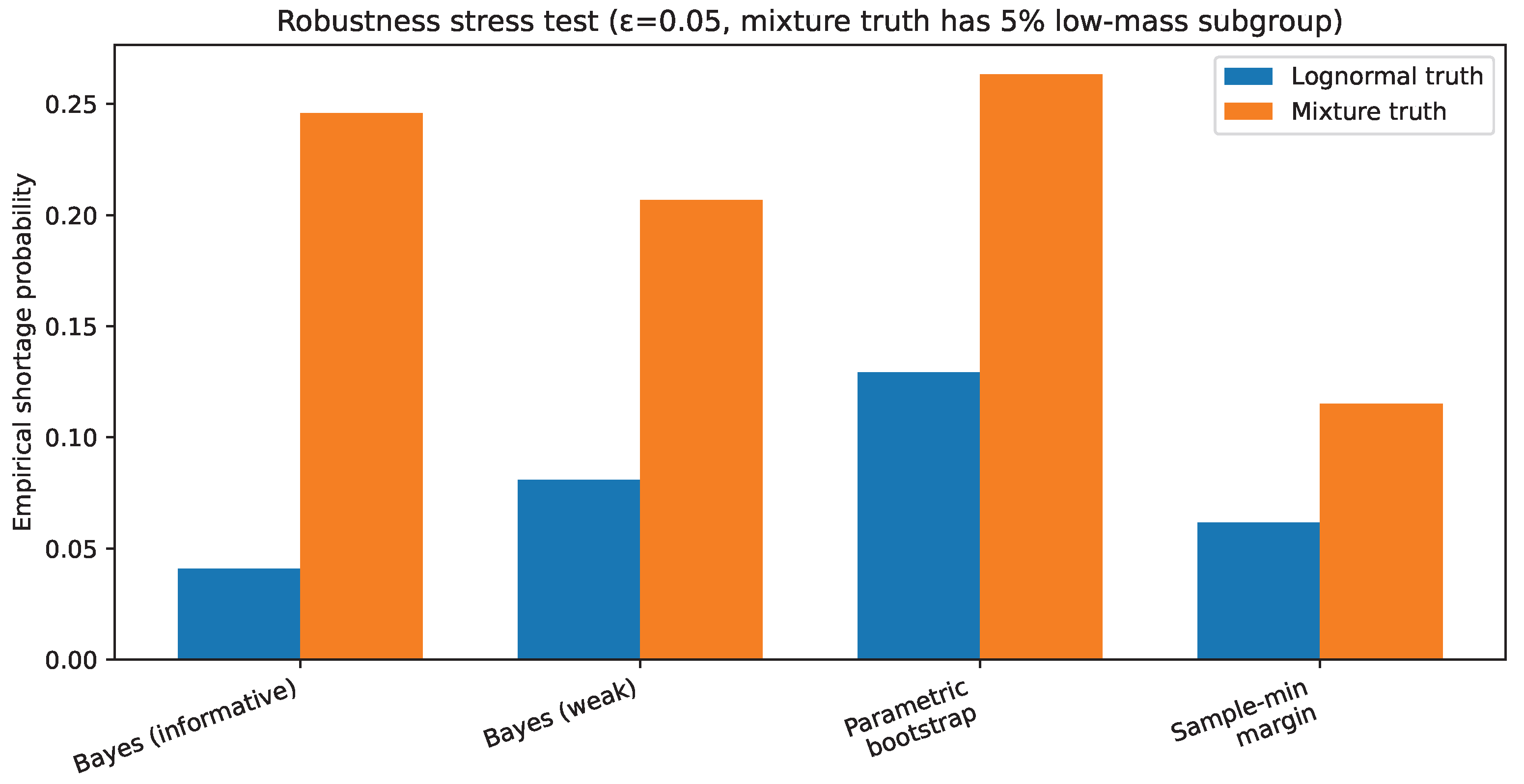
If cones from different lots, suppliers, or creel positions are pooled as if fully exchangeable when a low-mass subgroup is actually present, the predictive minimum can be biased upward and the decision rule becomes optimistic. The mixture stress test reported later in Section 6.7 is an explicit sensitivity check of this failure mode: the informative-prior Bayesian shortage rate rises from 0.041 under the baseline benchmark to 0.246 under the low-mass subgroup scenario. This indicates that the rule is much more sensitive to unmodeled subgroup heterogeneity than to ordinary within-group sampling noise, and it motivates stratified sampling or hierarchical models whenever such structure is operationally known.

2.4. Methods from the Literature

Before presenting the proposed Bayesian rule, we briefly position the main comparison methods from the literature that are later implemented in Section 5. The comparison set spans four complementary classes: a shop-floor heuristic based on the smallest observed cone, a parametric bootstrap analogue of the lognormal model, a distribution-free tolerance approach, and a lower-tail extreme-value fit.

These methods are included because they represent, respectively, operational simplicity, parametric frequentist uncertainty propagation, guarantee-based conservatism, and tail-focused modeling. Their detailed formulas are given later only to document the exact implementations used in the numerical study.

3. Bayesian Model in Log Space

3.1. Lognormal Likelihood

Residual cone masses are positive and often right-skewed; a lognormal model is therefore a natural baseline. In the present paper it is used as a pragmatic baseline rather than as a claim that it is the only admissible positive-support family. The choice is motivated by three considerations: the log transform places the problem on an interpretable location-dispersion scale for small samples, the Normal–Inverse-Gamma prior gives closed-form posterior updating, and the resulting posterior predictive minimum can be sampled efficiently for the chance-constrained rule. Gamma, Weibull, or log-skew-normal models are plausible alternatives, but with the small weighing budgets studied here, they introduce additional shape or skew parameters that are harder to identify robustly. For that reason, model adequacy is checked empirically through calibration, posterior predictive checks, and the heterogeneity stress test rather than being assumed a priori [16,17].

Let

$$Y_i=log{W}_i.$$

(4)

We assume

$$Y_i\mid \mu ,{\sigma }^2\sim \mathcal{N}(\mu ,{\sigma }^2),i=1,\dots ,N.$$

(5)

The parameters $(\mu ,{\sigma }^2)$ capture the location and dispersion of residual masses in log-space. Importantly, ${\sigma }^2$ is treated as unknown; assuming known dispersion can lead to systematically over-optimistic tail predictions when n is small.

3.2. Conjugate Normal–Inverse-Gamma Prior

We place a conjugate Normal–Inverse-Gamma prior on $(\mu ,{\sigma }^2)$:

$$\begin{array}{cc}\hfill {\sigma }^2& \sim \text{Inv-Gamma}({\alpha }_0,{\beta }_0),\hfill \end{array}$$

(6)

$$\begin{array}{cc}\hfill \mu \mid {\sigma }^2& \sim \mathcal{N}\left({\mu }_0,{\displaystyle \frac{{\sigma }^2}{{\lambda }_0}}\right),\hfill \end{array}$$

(7)

where $({\mu }_0,{\lambda }_0,{\alpha }_0,{\beta }_0)$ are hyperparameters. This prior supports transparent elicitation from historical warping runs: $({\mu }_0,{\sigma }_0)$ can be set from a historical log-mean and log-standard deviation, while $({\lambda }_0,{\alpha }_0)$ encode an “equivalent sample size” reflecting prior strength [16,18].

A practical elicitation recipe is to compute a historical log-space mean ${\overline{y}}_h$ and variance $s_h^2$ from comparable runs, set ${\mu }_0={\overline{y}}_h$, and choose ${\alpha }_0>1$ with ${\beta }_0=({\alpha }_0-1)s_h^2$ so that the prior mean of ${\sigma }^2$ matches the historical variance. The parameter ${\lambda }_0$ controls how strongly the prior mean is trusted, while $2{\alpha }_0$ plays the same role for prior dispersion. When historical data are limited, recent but comparable runs can still be used to center ${\mu }_0$, but ${\lambda }_0$ and ${\alpha }_0$ should be kept small so that current measurements dominate. When historical data are unreliable or regime shifts are suspected, the informative prior should be down-weighted further and checked against the weak-prior analysis reported later in Section 5.4.

For example, suppose m comparable historical runs are available and each run r yields fitted lognormal summaries $({\widehat{\mu }}_r,{\widehat{\sigma }}_r^2)$. A simple empirical-Bayes recipe is: (i) set ${\mu }_0=m^{-1}{\sum }_{r=1}^m{\widehat{\mu }}_r$; (ii) compute ${\overline{v}}_h=m^{-1}{\sum }_{r=1}^m{\widehat{\sigma }}_r^2$; (iii) choose an effective historical weight $m_{\mathrm{eff}}\le m$ and set ${\lambda }_0=m_{\mathrm{eff}}$ and ${\alpha }_0=2+m_{\mathrm{eff}}/2$; and (iv) set ${\beta }_0=({\alpha }_0-1){\overline{v}}_h$ so that the prior mean of ${\sigma }^2$ matches the historical average dispersion. If the historical runs are heterogeneous or only weakly reliable, reduce $m_{\mathrm{eff}}$ toward a weak prior so that current weighings dominate.

Equations (8)–(11) below are the standard conjugate posterior updates for the Normal–Inverse-Gamma model; their derivation is omitted here and standard references are cited for completeness. The formulas are retained only to keep the implementation self-contained [16,18].

Given a sample $y_{1:n}=log{w}_{1:n}$ with mean $\overline{y}$ and sum of squares $\sum {(y_j-\overline{y})}^2$, the posterior is also Normal–Inverse-Gamma with parameters

$$\begin{array}{cc}\hfill {\lambda }_n& ={\lambda }_0+n,\hfill \end{array}$$

(8)

$$\begin{array}{cc}\hfill {\mu }_n& ={\displaystyle \frac{{\lambda }_0{\mu }_0+n\overline{y}}{{\lambda }_n}},\hfill \end{array}$$

(9)

$$\begin{array}{cc}\hfill {\alpha }_n& ={\alpha }_0+{\displaystyle \frac{n}{2}},\hfill \end{array}$$

(10)

$$\begin{array}{cc}\hfill {\beta }_n& ={\beta }_0+{\displaystyle \frac{1}{2}}\sum _{j=1}^n{(y_j-\overline{y})}^2+{\displaystyle \frac{1}{2}}{\displaystyle \frac{{\lambda }_{0}n}{{\lambda }_n}}{(\overline{y}-{\mu }_0)}^2.\hfill \end{array}$$

(11)

3.3. Allowance Model

The allowance Z can be treated as deterministic ($Z=S$) or stochastic, e.g., $Z\sim \mathrm{Gamma}(k,\theta )$, estimated from machine logs of start/stop events and breakage counts. In the stochastic case, the decision rule integrates over both cone-mass uncertainty and allowance uncertainty. In the primary synthetic study reported in Section 5, the allowance is treated as fixed, with $Z=S=30$ m/end. The stochastic specification is retained as an extension for plants with sufficiently stable log data on start/stop and breakage losses.

A direct Gamma fit from machine logs can be obtained if comparable runs provide recorded extra consumed length values $z_1,\dots ,z_T$ (m/end). Let $\overline{z}$ and $s_z^2$ be their sample mean and variance. A simple method-of-moments fit uses $\widehat{k}={\overline{z}}^2/s_z^2$ and $\widehat{\theta }=s_z^2/\overline{z}$, after which each predictive simulation draws $Z\sim \mathrm{Gamma}(\widehat{k},\widehat{\theta })$. In practice, the fit should be stratified by style or machine state whenever those factors materially change downtime or breakage losses.

4. Risk-Limited Decision Rule

4.1. Posterior Predictive Minimum

Conditional on parameters $(\mu ,{\sigma }^2)$, the residual masses $W_i$ are i.i.d. lognormal, so the minimum $W_{min}={min}_i{W}_i$ has conditional CDF

$$Pr(W_{min}\le t\mid \mu ,{\sigma }^2)=1-{\left[1-F(t\mid \mu ,{\sigma }^2)\right]}^N,$$

(12)

where $F(·\mid \mu ,{\sigma }^2)$ is the lognormal CDF.

The key operational random variable is the capacity

$$C=\kappa W_{min}-Z,$$

(13)

which represents the maximum feasible useful length (m/end) once allowances are subtracted.

4.2. Quantile Policy

For a target shortage probability $\epsilon \in (0,1)$, we define the decision rule

$$x^{*}\left(w_{1:n}\right)=Q_{\epsilon }\left(C\mid w_{1:n}\right),$$

(14)

i.e., the $\epsilon$-quantile of the posterior predictive distribution of C. In Bayesian decision terms, this is a risk-limited policy: it selects the largest length consistent with a posterior predictive probability of completion of at least $1-\epsilon$.

This quantile rule is preferred because it solves the chance-constrained problem directly: maximizing x subject to $Pr(C<x\mid w_{1:n})\le \epsilon$ yields the same decision as taking the $\epsilon$-quantile of C. The rule also has a standard decision-theoretic interpretation. Under asymmetric linear loss, conservative under-planning ${(C-x)}_{+}$ and shortage-inducing over-planning ${(x-C)}_{+}$ receive different weights, and the Bayes action is a predictive quantile. For the usual piecewise-linear loss, choosing the $\epsilon$-quantile means that shortage is penalized relative to conservatism in the ratio $(1-\epsilon ):\epsilon$; for $\epsilon =0.05$, this corresponds to roughly a 19:1 penalty in favor of avoiding shortage. Because the expected remainder decreases as x increases, the quantile rule can therefore be read as the remainder-efficient decision within the class of plans satisfying the posterior predictive risk cap [12,19,20].

4.3. Efficient Sampling of $W_{min}$

A naive simulation of $W_{min}$ would draw N masses per posterior draw. Instead, we use an inverse-transform identity that samples the minimum in $O\left(1\right)$ time per draw.

Proposition 1.

Let $U\sim \mathrm{Uniform}(0,1)$ and define $q=1-{(1-U)}^{1/N}$. For lognormal parameters $(\mu ,{\sigma }^2)$,

$$W_{min}\stackrel{d}{=}exp\left(\mu +\sigma {\mathrm{\Phi }}^{-1}\left(q\right)\right),$$

(15)

where ${\mathrm{\Phi }}^{-1}$ is the standard normal quantile function.

Derivation. The minimum CDF satisfies $F_{min}\left(t\right)=1-{(1-F\left(t\right))}^N$. Setting $F_{min}\left(t\right)=U$ implies $F\left(t\right)=1-{(1-U)}^{1/N}=q$, so $t=F^{-1}\left(q\right)$. For a lognormal distribution, $F^{-1}\left(q\right)=exp(\mu +\sigma {\mathrm{\Phi }}^{-1}\left(q\right))$.

To reduce algorithmic detail in the main text, the pseudocode used in the simulations is moved to Appendix A; only the inverse-transform identity needed to sample the minimum is retained here. The pseudocode itself is unchanged.

With S posterior predictive draws, this shortcut makes the minimum-sampling step scale as O(S) rather than O(NS), because each draw uses one uniform variate and one normal quantile evaluation instead of simulating all cone masses explicitly. In the reference Python 3.13.5 implementation supplied in the supplementary material, the reported setting N = 480, n = 20, and S = 1200 required roughly 2 ms per decision after warm-up in our test environment, which is compatible with real-time decision support.

The inverse-transform shortcut relies on conditional independence between cone masses given $(\mu ,{\sigma }^2)$. If correlations arise from shared production conditions, a natural extension is to model $(log{W}_1,\dots ,log{W}_N)$ jointly, for example, with lot- or creel-level random effects or a multivariate normal covariance structure. The simulation step would then draw the full predictive vector (or the relevant latent effects) and compute $W_{min}$ from that joint draw rather than from a scalar marginal CDF. The decision rule itself is unchanged, but the computational cost reverts from $O\left(1\right)$ minimum sampling to joint-vector simulation unless an additional dependence structure is exploited [21].

5. Benchmark Methods

To contextualize the Bayesian policy, we compare it against several widely used or conceptually relevant alternatives.

A brief literature positioning of these benchmark methods is given earlier in Section 2.4; the present section retains the precise operational definitions used in the simulation study so that the comparison remains reproducible.

The benchmark set is deliberately chosen to span four complementary comparison classes: a shop-floor heuristic based on the smallest observed cone, a parametric frequentist analogue that retains the same lognormal assumption but replaces the prior with bootstrap resampling, a distribution-free tolerance approach representing guarantee-based practice, and a lower-tail extreme-value fit used as a stress-test baseline. This combination makes it possible to compare the proposed Bayesian rule against operational simplicity, parametric uncertainty propagation, distribution-free conservatism, and tail-focused modeling.

5.1. Sample-Minimum Margin Heuristic

A common rule is to base the decision on the smallest weighed cone and subtract an ad hoc margin:

$$x_{\min }=\kappa \underset{j}{min}{w}_j-S-M,$$

(16)

where $M\ge 0$ is a manually chosen “extra safety” margin. This approach is simple but does not explicitly propagate uncertainty about unweighed cones.

5.2. Parametric Bootstrap

A frequentist alternative is to fit a lognormal model to $w_{1:n}$, then propagate parameter uncertainty via bootstrap resampling [22]. Each bootstrap replicate yields $({\widehat{\mu }}^{\left(b\right)},{\widehat{\sigma }}^{\left(b\right)})$, from which one simulates $W_{min}^{\left(b\right)}$ and constructs $C^{\left(b\right)}=\kappa W_{min}^{\left(b\right)}-S$. The decision is $x_{\mathrm{boot}}^{*}={\mathrm{Quantile}}_{\epsilon }\left(\left\{C^{\left(b\right)}\right\}\right)$.

5.3. Distribution-Free Tolerance Bound and Sample Size Feasibility

If one requires a distribution-free guarantee with confidence $\gamma$ (e.g., 0.95) for the per-cone survival probability $p={(1-\epsilon )}^{1/N}$, Wilks’ result implies that using the sample minimum as a one-sided tolerance bound requires

$$1-p^n\ge \gamma ,\mathrm{i}.\mathrm{e}.,n\ge {\displaystyle \frac{log(1-\gamma )}{log\left(p\right)}}.$$

(17)

For large N, p is extremely close to 1, making n prohibitively large [23]. This provides a practical justification for adopting parametric modeling (with diagnostics) rather than insisting on distribution-free guarantees.

5.4. Extreme-Value Tail Fit (POT)

To explore tail-focused modeling, we also report a peaks-over-threshold (POT) baseline for the lower tail, using generalized Pareto theory [24,25,26]. With small n, such fits can be unstable; we treat POT as a stress-test baseline rather than a default recommendation.

6. Synthetic Case Study and Results

6.1. Synthetic Data Generation and Scope

Because proprietary warping logs are often confidential, we report an industrial-like synthetic study designed to mimic realistic magnitudes and variability. The synthetic experiments are fully reproducible; the code and generated CSV tables are included in the supplementary folder of this manuscript package.

The synthetic datasets and the associated graphs were not numerically generated by a generative-AI model. They were produced by author-executed Python simulations and plotting scripts implementing the probability models, parameter values, and Monte Carlo design stated in this section and in the supplementary code.

Within the scope of the present manuscript, a public cone-level case study with residual-mass measurements and end-out outcomes was not available, so the reproducible synthetic benchmark is used as the reference case for method validation. The synthetic design exposes the data-generating mechanism and therefore allows for direct assessment of shortage calibration and remainder across repeated runs.

The practical relevance of this synthetic benchmark is that it reproduces an industrially plausible decision scale—hundreds of cones, small weighing budgets, positive right-skewed residual masses, and a stress scenario with a small low-mass subgroup—while remaining fully auditable. It is used here as a controlled methodological benchmark rather than as a substitute for future plant validation on plant logs.

To improve the traceability of the figures, the supplementary package now provides the numerical outputs underlying the main frontiers and sample-size curves together with additional baseline histograms for cone masses, predictive minima, and mean remainders. These materials make the summarized plots directly reproducible and easier to interpret.

Unless otherwise stated, we consider $N=480$ cones (ends), a sample size $n=20$, yarn conversion $\kappa =40,000$ m/kg (e.g., Nm 40), and allowance $Z=S=30$ m/end. Residual masses are generated from a lognormal distribution with log-parameters $\mu =-2.919$ and $\sigma =0.3$ (kg units), calibrated so that the 5% quantile of the true population minimum corresponds to a last-band length on the order of 650–700 m/end.

These parameter values were chosen by back-calibration to a plausible operating scale rather than as universal constants. The selected $\mu =-2.919$ implies a median residual mass of about 0.054 kg, and together with $\sigma =0.3$ it gives a mean of about 0.056 kg. For $N=480$, $\kappa =40,000$ m/kg, and $S=30$ m/end, the resulting 5 percent quantile of the true capacity C is about 681 m/end. This places the benchmark in the same order of magnitude as the last-band decisions studied here while keeping moderate right-skewness.

6.2. Risk–Waste and Risk–Length Frontiers

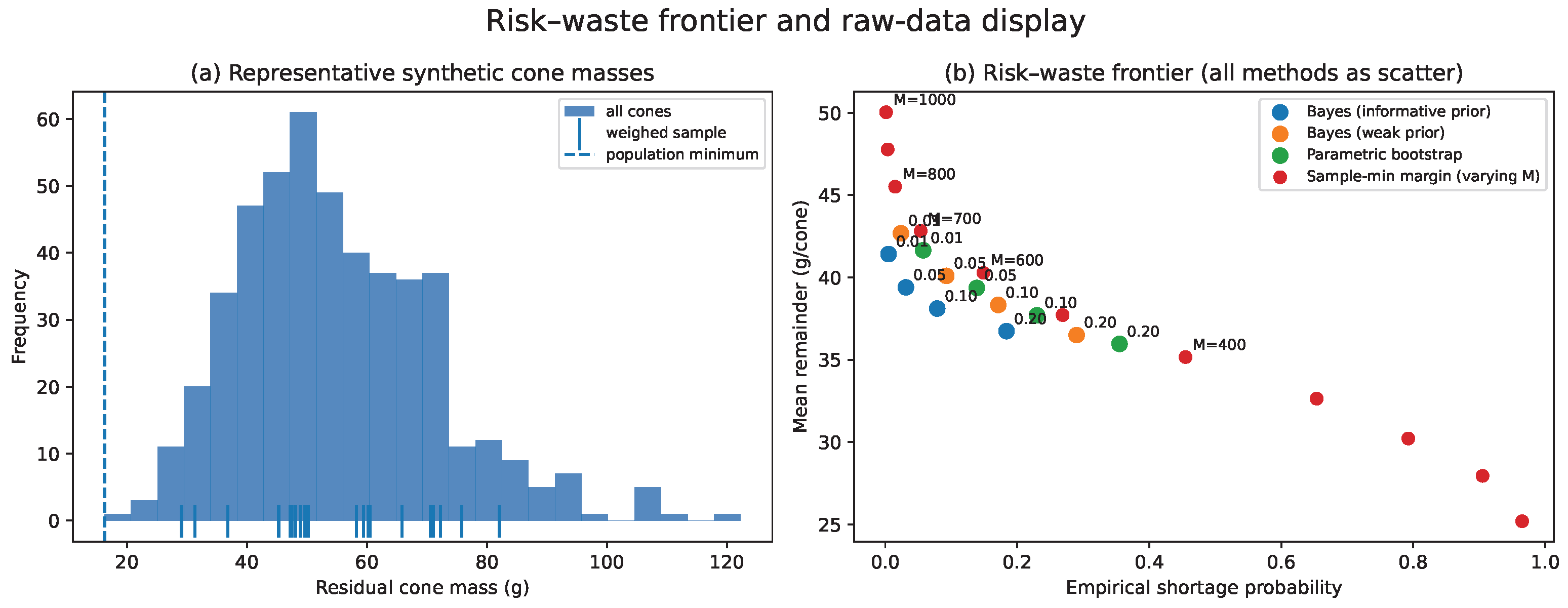
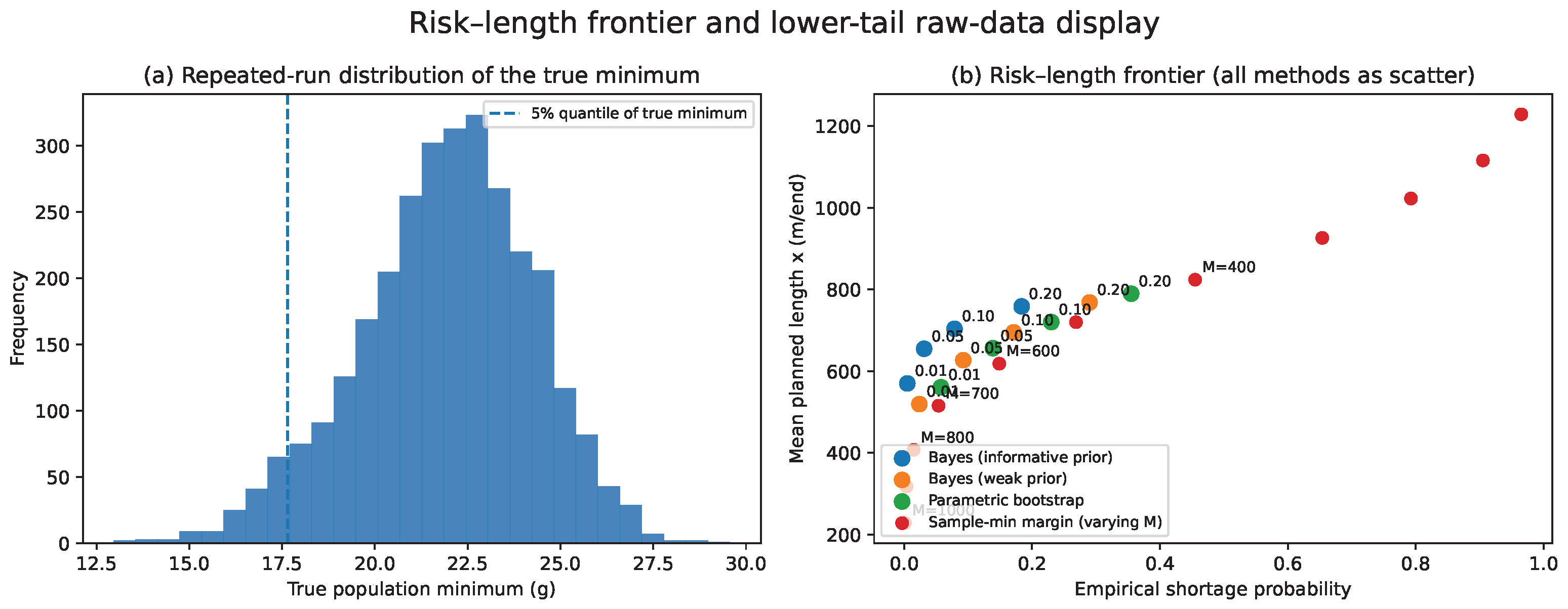
Panels (a) of Figure 2 and Figure 3 show raw synthetic distributions that ground the later comparison: a representative cone-mass histogram and the repeated-run distribution of the true population minimum. Panels (b) then report the results obtained with literature baselines and the proposed Bayesian rule on the same synthetic design.

Each point on the frontier is obtained by repeating the same planning rule over many synthetic runs, and then recording the realized shortage probability together with the corresponding mean remainder or planned length. The plotted frontiers are therefore Monte Carlo summaries rather than analytical curves, and the underlying numerical outputs are provided in the supplementary tables. For display consistency, all methods are now represented as scatter points rather than mixing point and line styles.

Figure 2 shows the empirical risk–waste frontier obtained by varying $\epsilon$ in the Bayesian policy and varying M in the sample-minimum heuristic. Figure 3 shows the corresponding risk–length trade-off.

Table 1. Bayesian (informative prior) risk–waste frontier summary (lognormal synthetic truth).

Target $\mathit{\epsilon }$	Mean x (m/End)	Empirical Shortage	Mean Remainder (g/Cone)
0.01	569.9	0.005	41.4
0.05	654.8	0.031	39.4
0.10	703.7	0.079	38.1
0.20	758.5	0.184	36.7

summarizes the Bayesian informative-prior frontier numerically. These tabulated values are the numerical counterparts of the informative-prior Bayesian points shown in the frontier displays of Figure 2 and Figure 3, so the reader can connect each target $\epsilon$ directly to its planned length and mean remainder.

Default Choice of the Target Risk

The frontier values explain why a 5 percent target shortage probability is used as the default operating point in later comparisons. Relative to a 1 percent target, the 5 percent target increases the planned band length by about 85 m/end and lowers the mean remainder, while the empirical shortage in the informative-prior Bayes policy remains below the nominal threshold. By contrast, 10 percent and 20 percent targets lead to substantially larger increases in realized shortage.

6.3. Calibration

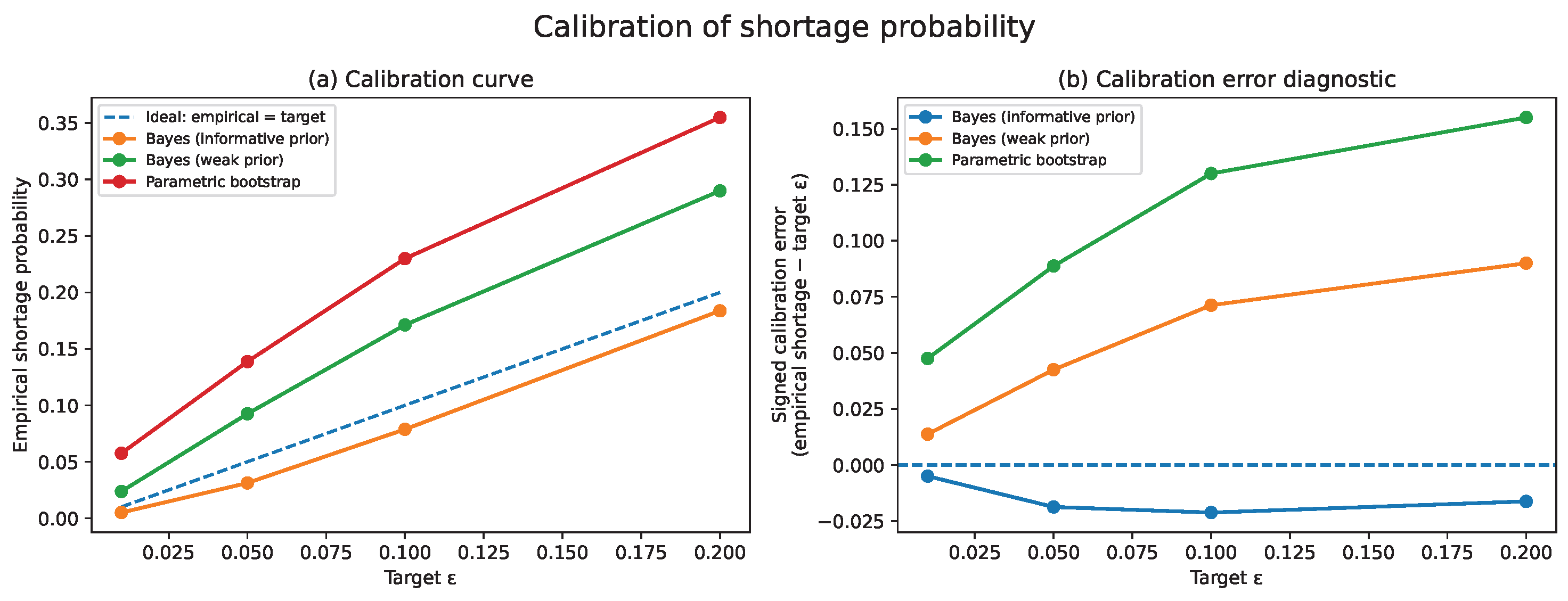
Figure 4 compares the empirical shortage probability to the target $\epsilon$ for the Bayesian and bootstrap policies. The informative prior reduces variability in the selected x and improves calibration for small n relative to weak priors; nevertheless, mild conservatism is expected because posterior predictive quantiles do not guarantee exact frequentist calibration.

Calibration is assessed here as a diagnostic rather than by fitting an additional optimization criterion. For each target value, the signed calibration error is $e\left(\epsilon \right)={\widehat{p}}_{\mathrm{short}}\left(\epsilon \right)-\epsilon$, estimated over repeated synthetic runs; the companion panel reports this signed discrepancy directly. No separate minimization is performed, because the decision rule is fixed once the posterior predictive quantile policy is specified.

The informative-prior curve remains slightly below the ideal line at the smallest target values because prior regularization and finite-sample uncertainty make the policy mildly conservative under repeated sampling. The later use of the 5 percent target is therefore motivated by the broader production-risk compromise seen in the frontier summary, rather than by exact alignment with the ideal line at any single target value.

From a frequentist repeated-sampling perspective, posterior predictive quantiles need not be exactly calibrated in finite samples, so a small bias is expected when n is limited. For practitioners who require a nominal service level, a practical option is replay or bootstrap calibration of $\epsilon$: select an operational ${\epsilon }_{\mathrm{op}}$ such that historical replay or plant simulation reproduces the desired realized shortage rate in the relevant regime. In the present informative-prior benchmark, the nominal $\epsilon =0.05$ already yields an empirical shortage of about 3.1%, so the policy is mildly conservative and no additional bias correction was applied in the main results. In a risk-averse industrial setting, this mild conservatism can be desirable, because the nominal $\epsilon =0.05$ policy delivers an additional buffer against end-outs while remaining operationally simple. This type of calibration becomes more relevant when weak priors or stronger misspecification are expected [16,27].

6.4. Benchmark Comparison at $\epsilon =0.05$

Accuracy is assessed here against synthetic truth with known generating parameters, so the reference shortage and remainder values are directly observable across repeated runs. This design was retained because the present manuscript does not include a public cone-level benchmark with residual-mass measurements and end-out outcomes suitable for a like-for-like statistical comparison.

For presentation, the literature baselines are interpreted first and the Bayesian policies are then compared against them under exactly the same synthetic runs.

Table 2. Method comparison at target $\epsilon =0.05$ under lognormal synthetic truth ($N=480$, $n=20$).

Method	Mean x (m/End)	Empirical Shortage	Mean Remainder (g/Cone)	SD(x)
Bayes (informative prior)	655.5	0.041	39.3	33.6
Bayes (weak prior)	629.2	0.081	40.0	118.7
Parametric bootstrap	658.6	0.129	39.3	133.7
Sample-min margin (M = 700 m)	517.4	0.062	42.8	186.5
EVT-POT (MoM)	631.4	0.348	40.0	408.2

compares methods at target $\epsilon =0.05$ under lognormal truth. The Bayesian informative-prior policy achieves the lowest remainder among the compared methods while keeping shortages close to the target. The tuned sample-minimum heuristic must subtract a large margin ($M=700$ m) to approach similar risk, increasing the remainder.

The higher shortage probability of the parametric bootstrap relative to the informative-prior Bayesian rule is driven by both parameter-uncertainty propagation and prior regularization, but the comparison in Table 2 suggests that prior regularization is the dominant effect here. The weak-prior Bayesian rule already propagates uncertainty while applying little shrinkage, and it shows both higher shortage and much larger SD$\left(x\right)$ than the informative-prior rule. The bootstrap amplifies this instability because repeated refits from $n=20$ observations generate highly variable lower-tail parameter estimates. In other words, both methods acknowledge parameter uncertainty, but the informative prior stabilizes the predictive lower tail enough to materially improve risk control in this small-sample regime.

6.5. Sample Size and Distribution-Free Feasibility

6.5.1. Distribution-Free Feasibility

Table 3. Wilks distribution-free sample-size requirement for per-cone survival $p={(1-\epsilon )}^{1/N}$ at confidence $\gamma =0.95$ (Equation (17)).

N	$\mathit{\epsilon }$	$\mathit{p}={(1-\mathit{\epsilon })}^{1/\mathit{N}}$	Required n
120	0.01	0.999916	35,769
120	0.05	0.999573	7009
120	0.10	0.999122	3412
240	0.01	0.999958	71,538
240	0.05	0.999786	14,017
240	0.10	0.999561	6824
480	0.01	0.999979	143,075
480	0.05	0.999893	28,034
480	0.10	0.999781	13,648

reports Wilks’ required sample sizes for a distribution-free one-sided tolerance bound based on the sample minimum (confidence $\gamma =0.95$). Even for moderate N, the required n is orders of magnitude larger than feasible in production, supporting the use of parametric/historical models paired with diagnostics.

6.5.2. Effect of n on Risk and Waste

Table 4. Effect of sample size n on performance (Bayesian weak prior, target $\epsilon =0.05$).

n	Mean x (m/End)	Empirical Shortage	Mean Remainder (g/Cone)	SD (x)
5	585.6	0.107	41.1	183.3
10	607.9	0.098	40.5	158.2
20	634.2	0.083	39.8	123.4
30	638.9	0.069	39.8	101.3
40	651.7	0.079	39.4	93.9
50	658.4	0.069	39.3	83.3
60	662.0	0.063	39.2	75.8
70	664.5	0.056	39.2	67.2
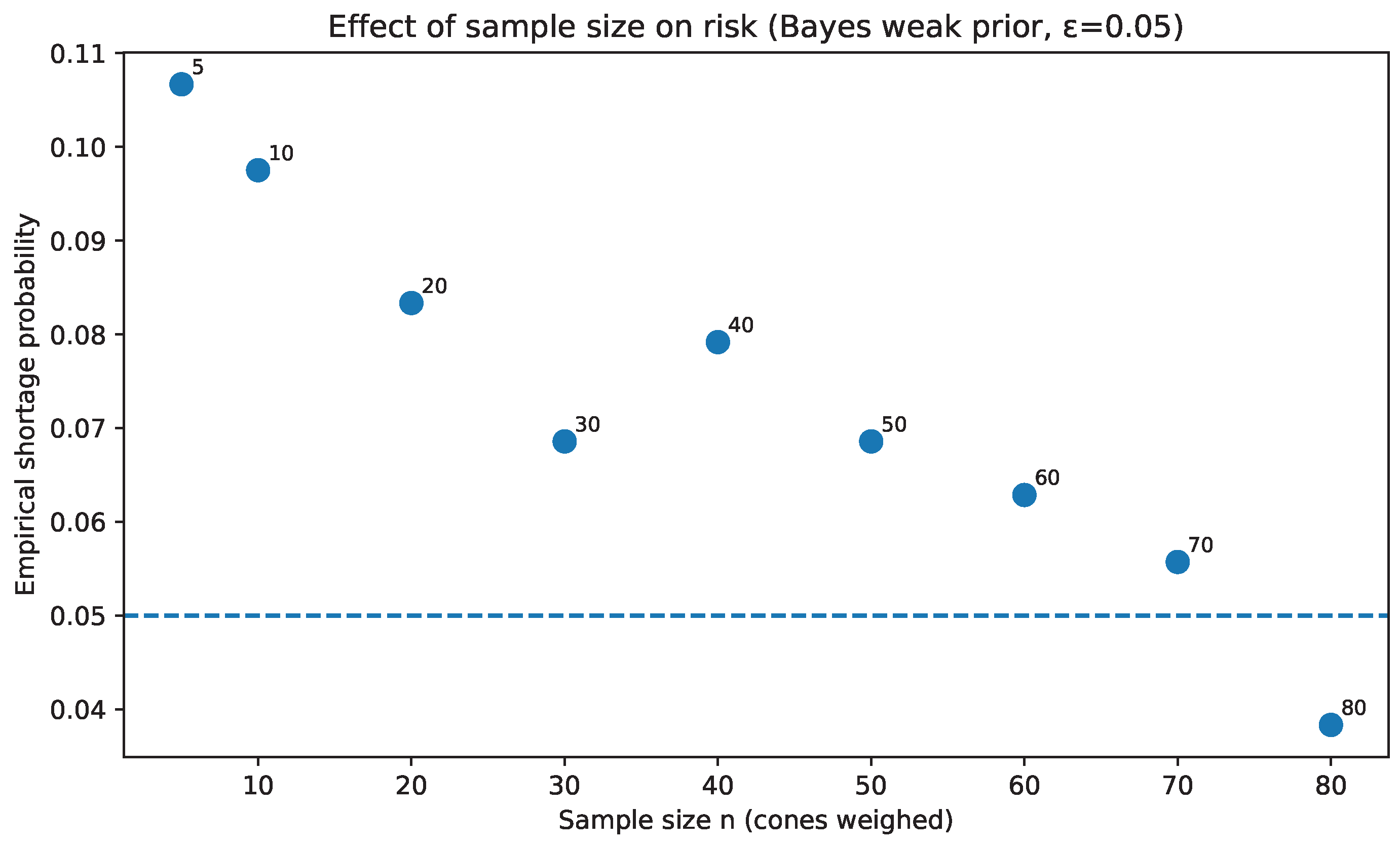
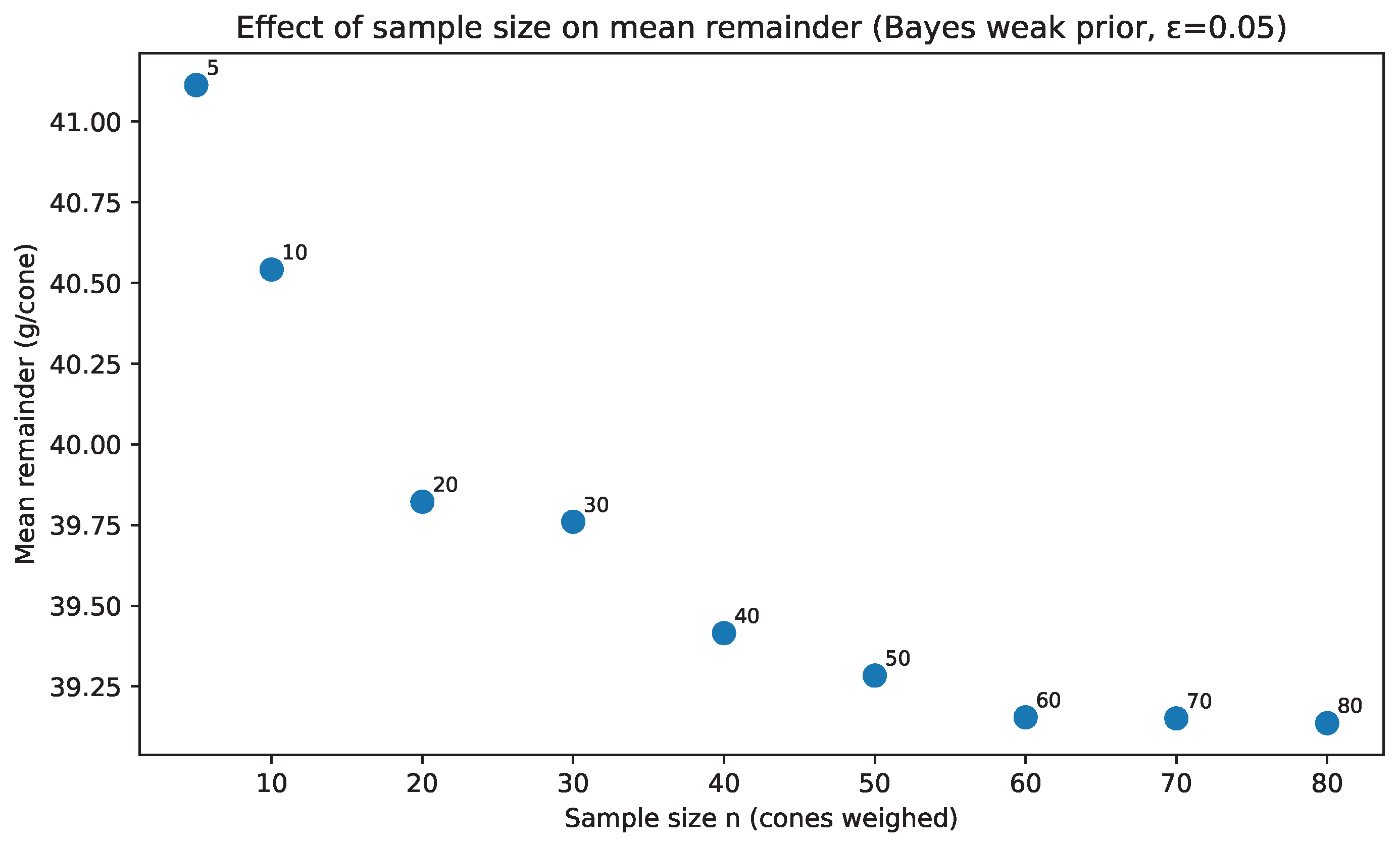
80	663.6	0.038	39.1	65.2

and Figure 5 and Figure 6 include additional sample sizes between 40 and 80 so that the crossing of the 5 percent target is shown directly rather than inferred from interpolation. In the updated grid, the empirical shortage remains above 5 percent at $n=70$ and falls below 5 percent at $n=80$.

If the cost of weighing an additional cone is not constant—for example, because the marginal downtime cost rises during changeovers—the operating choice of n can be formalized by adding a sampling-cost term $c\left(n\right)$ to the performance study. A simple criterion is to choose n by minimizing a net operating loss such as $\mathbb{E}\left[R_n\right]+\lambda Pr(\mathrm{shortage}\mid n)+c\left(n\right)$, or equivalently by increasing n only while the marginal reduction in shortage/remainder cost exceeds the extra weighing cost. This extension does not change the decision rule for a fixed n; it only changes how the sample size itself is selected [12,20].

6.6. Posterior Predictive Checks

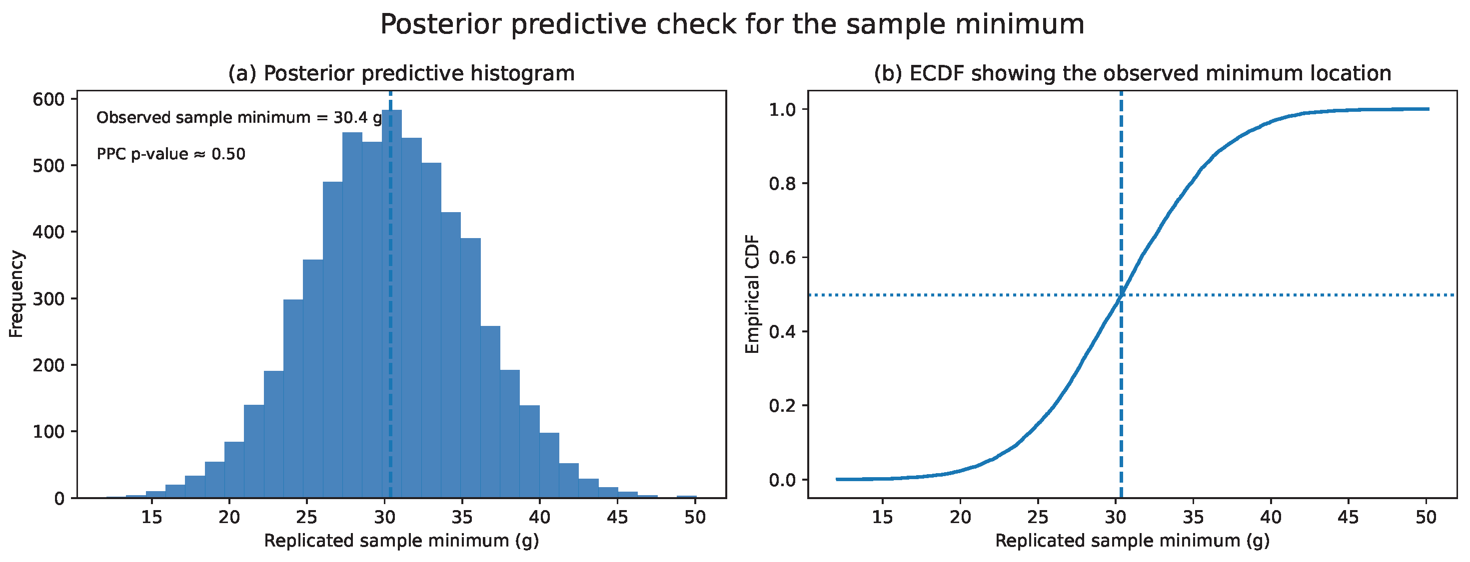
Posterior predictive checks (PPCs) can be targeted to the lower tail by comparing observed and replicated sample minima [15]. In Figure 7, the dashed vertical marker denotes the minimum observed in the actual weighed sample, not a minimum of the histogram itself; the added ECDF panel makes this interpretation explicit. Extreme PPC p-values near 0 or 1 may indicate tail misfit or biased sampling.

6.7. Robustness Stress Test: Mild Heterogeneity

To illustrate sensitivity to unmodeled heterogeneity, we consider a finite-mixture stress test in which 5 percent of cones belong to a lower-mass subgroup with a mean residual mass of 0.035 kg, while the remaining cones follow the baseline lognormal component; both components use the same log-scale dispersion. This is a deliberately adverse but transparent misspecification scenario of the type commonly represented with mixture models [28].

Table 5. Stress test under mild mixture heterogeneity (target $\epsilon =0.05$). The mixture truth uses a 5 percent low-mass subgroup with mean residual mass 0.035 kg and common log-scale dispersion.

Method	Mean x (m/End)	Empirical Shortage	Mean Remainder (g/Cone)	SD (x)
Bayes (informative prior)	640.9	0.246	38.6	39.5
Bayes (weak prior)	583.8	0.207	40.1	126.6
Parametric bootstrap	608.8	0.263	39.4	141.0
Sample-min margin (M = 700 m)	429.1	0.115	43.9	207.8
EVT-POT (MoM)	541.8	0.370	41.1	396.0

reports performance under this stress test, and Figure 8 compares shortage rates for the selected methods under lognormal vs. mixture truth. In such settings, increasing n, stratifying the sample, or moving to hierarchical/mixture models is advisable.

7. Practical Deployment and Limitations

The proposed framework is intended to be operational: a small sample of cone masses is weighed, yarn count is known (thus $\kappa$), and a single $x^{*}$ is computed for the final band. Practical deployment considerations include:

Sampling plan. If sampling is biased (e.g., avoiding cones suspected to be low), the policy will be optimistic. Stratified sampling by creel region, lot, or package history can reduce the chance of missing low-mass subpopulations.

Prior elicitation and drift monitoring. Informative priors improve stability for small n but can be dangerous under regime shifts (e.g., a new supplier lot). PPC diagnostics and rolling re-estimation can detect drift.

Allowance estimation. When start/stop losses and breakage allowance vary substantially across styles, modeling Z stochastically (from logs) is preferable to a fixed margin.

Model misspecification. If the lower tail is heavier than implied by a lognormal model, minimum predictions can be optimistic. EVT-based tail modeling and mixture/hierarchical models offer principled extensions [24,25,26,29]. The stress test illustrates how rare low-mass cones can dominate failure probability when N is large. A concrete robustification that stays within the same chance-constrained framework is to replace the single-component predictive model by a two-component lognormal mixture with a small low-mass component and then compute the same predictive $\epsilon$-quantile of capacity. If practitioners prefer to keep a single-component likelihood, an alternative is to use a heavier-tailed or less concentrated prior on ${\sigma }^2$ so that posterior predictive lower tails widen rather than being forced toward an overconfident narrow scale [16,28]. Related predictive model-comparison tools, Monte Carlo implementations, and Bayesian or semi-parametric extreme-value formulations are discussed in [30,31,32,33,34,35].

Structured extensions. When plant metadata are available, a natural next step is a hierarchical Bayesian model with lot-, supplier-, or creel-position effects and covariates such as yarn count, package age, or machine settings. Such models relax unconditional exchangeability by borrowing strength only within comparable groups. A second extension is adaptive sampling: if the posterior shortage risk at the provisional $x^{*}$ lies close to the decision threshold, or if PPC diagnostics indicate lower-tail tension, additional cones can be weighed selectively before locking the final-band length. A simple sequential strategy is to compute an initial $x^{*}$ from the first weighing batch and then trigger a second batch only if the initial PPC indicates poor lower-tail fit or if the provisional decision remains too close to the operational risk limit [21].

Contribution Summary

• A chance-constrained formulation of last-band planning linking yarn count, residual cone mass, and allowances to the completion event;
• A conjugate Bayesian model for residual cone mass in log-space, enabling analytic posterior updates under limited sampling;
• An efficient posterior predictive sampler for the population minimum $W_{min}$ avoiding $O\left(N\right)$ simulations per posterior draw;
• A quantile-based risk-limited decision rule for selecting x from the posterior predictive distribution of a capacity variable;
• Benchmark methods (margin heuristic, bootstrap, Wilks tolerance bound, and EVT tail fit) together with a sample-size feasibility bound.

8. Conclusions

We presented a Bayesian chance-constrained framework for selecting the final-band length in sectional warping under limited cone weighing. The approach models residual mass in log-space with a conjugate Normal–Inverse-Gamma prior, derives the posterior predictive distribution of the population minimum, and selects the final-band length as a lower posterior predictive quantile of a capacity variable to enforce a specified shortage probability. Benchmarks and a synthetic case study demonstrate that the Bayesian policy can reduce the remainder relative to a tuned sample-minimum heuristic while providing an explicit risk–waste frontier. We also showed that distribution-free guarantees for the minimum would require weighing orders of magnitude more cones than is feasible, motivating parametric modeling combined with diagnostics and prior sensitivity analysis.

Three practical conclusions follow from the revised study. First, the informative-prior Bayesian policy offers the best overall compromise in the benchmarked lognormal setting, because it keeps shortage risk close to the target while reducing remainder and substantially stabilizing the chosen length relative to weaker-prior and bootstrap alternatives. Second, the updated sample-size analysis shows directly that, under the synthetic weak-prior setting studied here, the empirical shortage probability remains above 5 percent at $n=70$ and drops below that target at $n=80$, so the threshold cannot be inferred reliably from a sparse grid. Third, the explicit mixture stress test confirms that hidden low-mass subpopulations can dominate failure probability, which supports the operational recommendations of stratified sampling, drift monitoring, and future hierarchical or mixture extensions.

References

- Adanur, S. Handbook of Weaving; CRC Press: Boca Raton, FL, USA, 2000. [Google Scholar]
- Lord, P.R.; Mohamed, M.H. Weaving: Conversion of Yarn to Fabric; Merrow: Watford, UK, 1982. [Google Scholar]
- Hu, J.; Babu, K.M. Weaving preparation: Warping, sizing, drawing-in and tying. Text. Asia 2007, 38–39, 27–33. [Google Scholar]
- Eren, R.; Suvari, F.; Celik, O. Mathematical analysis of motion control in sectional warping machines. Text. Res. J. 2018, 88, 133–143. [Google Scholar] [CrossRef] [Scilit]
- Eren, R.; Celik, O.; Suvari, F.; Koksal, S.A. Measurement and analysis of winding thickness variations in sectional warping process. Int. J. Cloth. Sci. Technol. 2018, 30, 772–783. [Google Scholar] [CrossRef] [Scilit]
- Hussain, D.; Figueiredo, M.C. Improving the time-based performance of the preparatory stage in textile manufacturing process with value stream mapping. Bus. Process Manag. J. 2023, 29, 801–837. [Google Scholar] [CrossRef] [Scilit]
- Tu, L.; Guo, M.R.; Wang, J.; Gao, W. Dynamic tension control for warp beams on sizing machine based on unwinding length monitoring. Text. Res. J. 2024, 94, 1126–1144. [Google Scholar] [CrossRef] [Scilit]
- Tu, L.; Guo, M.R.; Wang, J.; Gao, W. Warp yarn tension coupling models and fuzzy PID control for enhancing warp beam unwinding tension stability in sizing machines. J. Ind. Text. 2024, 54, 15280837241301709. [Google Scholar] [CrossRef] [Scilit]
- Eren, R.; Kılıç, S.; Atalay, Ö. Development of an individual warp beam tension control system for warp assembling machines in direct warp preparation. J. Eng. Fibers Fabr. 2025, 20, 15589250251313609. [Google Scholar] [CrossRef] [Scilit]
- Idzik, M.; Rybicki, T. Real-Time Prediction of the Yarn Break Position Using Vibration Measurement. Sensors 2025, 25, 299. [Google Scholar] [CrossRef] [Scilit] [PubMed]
- Prékopa, A. Stochastic Programming; Springer: Dordrecht, The Netherlands, 1995. [Google Scholar]
- Raiffa, H.; Schlaifer, R. Applied Statistical Decision Theory; Division of Research, Graduate School of Business Administration, Harvard University: Boston, MA, USA, 1961. [Google Scholar]
- Arnold, B.C.; Balakrishnan, N.; Nagaraja, H.N. A First Course in Order Statistics; SIAM: Philadelphia, PA, USA, 2008. [Google Scholar]
- David, H.A.; Nagaraja, H.N. Order Statistics, 3rd ed.; Wiley: Hoboken, NJ, USA, 2003. [Google Scholar]
- Gelman, A.; Meng, X.-L.; Stern, H. Posterior predictive assessment of model fitness via realized discrepancies. Stat. Sin. 1996, 6, 733–807. [Google Scholar]
- Gelman, A.; Carlin, J.B.; Stern, H.S.; Dunson, D.B.; Vehtari, A.; Rubin, D.B. Bayesian Data Analysis, 3rd ed.; Chapman and Hall/CRC: Boca Raton, FL, USA, 2013. [Google Scholar]
- Aitchison, J.; Brown, J.A.C. The Lognormal Distribution, with Special Reference to Its Uses in Economics; Cambridge University Press: Cambridge, UK, 1957. [Google Scholar]
- Bernardo, J.M.; Smith, A.F.M. Bayesian Theory; Wiley: Chichester, UK, 1994. [Google Scholar]
- Gneiting, T. Quantiles as optimal point forecasts. Int. J. Forecast. 2011, 27, 197–207. [Google Scholar] [CrossRef] [Scilit]
- Berger, J.O. Statistical Decision Theory and Bayesian Analysis, 2nd ed.; Springer: New York, NY, USA, 1985. [Google Scholar]
- Gelman, A.; Hill, J. Data Analysis Using Regression and Multilevel/Hierarchical Models; Cambridge University Press: Cambridge, UK, 2007. [Google Scholar]
- Efron, B.; Tibshirani, R.J. An Introduction to the Bootstrap; Chapman and Hall: New York, NY, USA, 1993. [Google Scholar]
- Wilks, S.S. Determination of sample sizes for setting tolerance limits. Ann. Math. Stat. 1941, 12, 91–96. [Google Scholar] [CrossRef] [Scilit]
- Coles, S. An Introduction to Statistical Modeling of Extreme Values; Springer: London, UK, 2001. [Google Scholar]
- Embrechts, P.; Klüppelberg, C.; Mikosch, T. Modelling Extremal Events for Insurance and Finance; Springer: Berlin, Germany, 1997. [Google Scholar]
- de Haan, L.; Ferreira, A. Extreme Value Theory: An Introduction; Springer: New York, NY, USA, 2006. [Google Scholar]
- Rubin, D.B. Bayesianly justifiable and relevant frequency calculations for the applied statistician. Ann. Stat. 1984, 12, 1151–1172. [Google Scholar] [CrossRef] [Scilit]
- McLachlan, G.; Peel, D. Finite Mixture Models; Wiley: New York, NY, USA, 2000. [Google Scholar]
- Stephenson, A.; Tawn, J. Bayesian inference for extremes: Accounting for the three extremal types. Extremes 2004, 7, 291–307. [Google Scholar] [CrossRef] [Scilit]
- Vehtari, A.; Gelman, A.; Gabry, J. Practical Bayesian model evaluation using leave-one-out cross-validation and WAIC. Stat. Comput. 2017, 27, 1413–1432. [Google Scholar] [CrossRef] [Scilit]
- Robert, C.P.; Casella, G. Monte Carlo Statistical Methods, 2nd ed.; Springer: New York, NY, USA, 2004. [Google Scholar]
- Coles, S.G.; Tawn, J.A. A Bayesian analysis of extreme rainfall data. J. R. Stat. Soc. Ser. C Appl. Stat. 1996, 45, 463–478. [Google Scholar] [CrossRef] [Scilit]
- Pickands, J., III. Statistical inference using extreme order statistics. Ann. Stat. 1975, 3, 119–131. [Google Scholar] [CrossRef] [Scilit]
- Smith, R.L. Estimating tails of probability distributions. Ann. Stat. 1987, 15, 1174–1207. [Google Scholar] [CrossRef] [Scilit]
- Hill, B.M. A simple general approach to inference about the tail of a distribution. Ann. Stat. 1975, 3, 1163–1174. [Google Scholar] [CrossRef] [Scilit]
Figure 1.
Schematic overview used in the Introduction: a random sample of cones is weighed to estimate the limiting residual mass before selecting the final-band length.
Figure 2.
Updated display for the lognormal synthetic benchmark. Panel (a) shows a representative raw histogram of cone residual masses together with the weighed sample marks and the population minimum. Panel (b) shows the empirical risk–waste frontier, with every method represented as scatter points.
Figure 3.
Updated display for the lognormal synthetic benchmark. Panel (a) shows the repeated-run distribution of the true population minimum. Panel (b) shows the corresponding risk–length frontier, with every method represented as scatter points.
Figure 4.
Calibration under lognormal synthetic truth. Panel (a) compares empirical shortage probability with the target . Panel (b) reports the signed calibration error , clarifying how calibration was diagnosed.
Figure 5.
Effect of sample size on empirical shortage probability (Bayesian weak prior, target ). The additional points between 40 and 80 show the threshold crossing directly, and the dashed horizontal line marks the nominal 5 percent target.
Figure 6.
Effect of sample size on mean remainder (Bayesian weak prior, target
) using the denser sample-size grid reported in