1. Introduction
Microalgae, being unicellular organisms, need sunlight, water, and a carbon source to grow [
1]. The cultivation of these organisms can be done in different ways, including via phototrophic, heterotrophic, mixotrophic, and photoheterotrophic methods, each presenting unique advantages and difficulties [
2]. These adaptable microorganisms can be used in creating third-generation biofuels, biopolymers. They can also be utilized in waste conversion to biofuels and bioproducts, especially when cultivated in a heterotrophic manner [
3]. Moreover, microalgae, especially marine microalgae, can play a role in sustainable development, specifically in the realm of biofuels [
4]. They also hold promise as a sustainable feed component for aquaculture [
5]. The economic feasibility of producing large-scale marine microalgal biofuels is still a challenge according to [
4].
Microalgae such as
Scenedesmus obliquus and
Chlorella minutissima have demonstrated efficient nitrogen and phosphorus removal from wastewater, along with the possibility of increased biomass and lipid generation [
6]. Intensive farming methods and utilizing waste products like aquaculture wastewater can help decrease water usage and improve lipid production [
7]. Two-stage cultivation techniques have been suggested to optimize both high biomass production and the concentration of specific compounds [
8]. In [
9], the impact of nitrogen and phosphorus on microalgal growth, biomass, lipid, and fatty acid production is emphasized. Additional research is required to enhance microalgal cultivation and harvesting techniques to achieve higher biomass production and lower expenses [
10].
Microalgae are a valuable source of bioactive compounds that have a wide range of commercial uses. These substances, such as antioxidants, carotenoids, lipids, polyunsaturated fatty acids, peptides, toxins, and sterols, are utilized in various industries like human nutrition, animal feed, cosmetics, and pharmaceutical production [
11]. Scaling up microalgal production is still a challenge, and additional research is required to fully exploit their commercial potential [
12]. Microalgae are being utilized more in the food and feed industries, as well as in biotechnological processes, pharmaceuticals, and cosmeceuticals, despite facing challenges [
13]. Due to their high metabolic flexibility, rapid growth, and capacity to generate valuable bioproducts, they are considered a promising source of bioactive compounds [
14]. One of the main challenges is determining the economic feasibility of producing microalgae for different purposes such as biofuel, food, and pharmaceuticals [
12]. Closed photobioreactors and open ponds are commonly used, with the former being more cost-effective [
15]. Floating photobioreactors are a cost-effective and energy-efficient solution, as stated by [
16]. Various harvesting techniques, including filtration, centrifugation, flocculation, and flotation, are employed, and there is a possibility of utilizing waste biomass as bioflocculants [
17]. Physicochemical parameters such as gaseous transfer, mixing, light demand, and temperature play a vital role in increasing biomass yield [
18]. This study emphasizes the potential of microalgae for producing valuable products for human health and nutrition, specifically focusing on their biochemical composition and large-scale cultivation [
19]. In [
20], the utilization of microalgae for treating nutrient-rich wastewater from agro-based industries is discussed, highlighting obstacles and possible optimization strategies.
Flat-plate reactors, conceptualized with transparent materials to optimize solar radiation utilization, are designed as narrow panels to achieve high area-to-volume ratios and volumetric biomass productivities [
21]. Demonstrating suitability for the photoautotrophic production of diverse microalgal species, such as
Chlorella vulgaris,
Nannochloropsis oculata, and
Scenedesmus ovalternus, flat-plate photobioreactors have yielded biomass production ranging from 1.11 to 7.5 g L
−1 [
22,
23,
24]. However, the productivities achieved in these PBRs are currently insufficient for scalable applications. Consequently, strategies have been developed to enhance productivity, such as mixotrophic production involving various microalgae and organic carbon sources. The authors of [
25] investigated biomass productivities in mixotrophic batch cultures of
Nannochloropsis gaditana in a flat-panel photobioreactor, demonstrating the alga’s ability to grow mixotrophically using glucose and glycerol. The maximum biomass productivity in mixotrophic batch cultures, utilizing either glucose or glycerol, was found to be identical at 170 g L
−1 day
−1. Additionally, Ref. [
26] isolated and cultivated
Monoraphidium sp. in a flat-panel photobioreactor for the treatment of synthetic dairy wastewater. The system supported microalgal growth, achieving a biomass productivity of 50 mg
−1 day
−1 and accumulating carbohydrate (228.8 mg g
−1), protein (88.8 mg mg
−1), and lipid content (25%). These findings underscore the potential of flat-panel photobioreactors in advancing microalgal cultivation for various applications.
Despite the technological advancements in microalgal biotechnology, optimizing algal growth and biomass production is essential for enabling efficient operation and process control. Mathematical modeling emerges as a valuable tool in achieving this optimization, where the impact of each process condition (such as light, carbon source, and temperature) is mathematically linked to key production parameters (including growth rate and productivity). This approach allows for the observation of the effects of changes in process conditions without the need for separate experimental testing, as noted by [
1,
27]. The modeling of algal growth kinetics plays a pivotal role in both estimating and optimizing production parameters, as well as controlling process conditions. Luenberger observers, a crucial instrument in control theory, have been effectively utilized in overseeing and regulating photobioreactors, specifically in the growth of microalgae and other photosynthetic microorganisms [
28,
29,
30]. These observers have been utilized for estimating nutrient concentration, monitoring internal substrate quota, and measuring variables that are not measurable online, thereby aiding in the progress of biotechnology [
31]. Luenberger observers are being used in photobioreactors to advance biotechnology, especially in growing microalgae and other photosynthetic organisms [
32]. These observers have demonstrated superior performance compared to other methods like the extended Kalman filter [
33] and are resilient to model uncertainties and measurement noise [
34]. They have also been utilized in creating super-twisting observers to monitor microalgal cultures [
29]. Model-free control designs have been proposed as more effective than input–output feedback linearizing control strategies for enhancing microalgal growth in photobioreactors. One study investigated the application of Luenberger observers in optimizing microalgal photobioreactor systems [
35].
Recent advances in nonlinear observer design and bioprocess monitoring have highlighted the importance of robust estimation strategies under strong nonlinearities, uncertainty, and limited sensing. In the context of nonlinear and bilinear systems, advanced observer structures have been proposed to ensure reliable state reconstruction, even in the presence of model mismatch and incomplete measurements [
36]. From a biological and physical perspective, nonlinear phenomena such as phototaxis, collective behavior, and instability mechanisms in microalgal suspensions have been experimentally and theoretically analyzed, revealing the intrinsic complexity of algal systems and the need for nonlinear modeling frameworks [
37].
Regarding photobioreactor monitoring, recent contributions have focused on online biomass estimation using limited measurements, emphasizing industrial applicability and real-time implementation [
38]. Nonlinear observer-based approaches have also been successfully applied to related bioprocesses, such as respiration rate estimation in wastewater treatment, demonstrating improved robustness compared with linear estimation techniques [
39]. Hybrid observer architectures combining asymptotic and Kalman-based strategies have further been proposed for microalgal growth estimation in closed photobioreactors, addressing noise sensitivity and uncertainty issues [
40].
These recent developments motivate the present work, which extends the current state of the art by proposing an integral-enhanced nonlinear observer specifically tailored for photobioreactor monitoring, offering improved robustness against constant disturbances and modeling uncertainty while relying on a reduced set of online measurements.
This study presents a new theoretical and practical design of an innovative observer model called the PI squared () Luenberger observer, designed specifically for use in photobioreactors. This observer model is notable for its innovative method of estimating the internal states of photobioreactors, which is essential for the optimal growth of microalgae. The observer improves state estimation accuracy in bioreactors by utilizing the strong and flexible features of () control to handle dynamic and uncertain conditions effectively. This advancement has the potential to greatly enhance the effectiveness and dependability of microalgal cultivation systems, representing a groundbreaking advancement in combining advanced control methods with bioprocess engineering.
Microalgal cultivation theory and photobioreactor applications are covered in
Section 1. This study will examine its goals and effects after this Introduction.
Section 2 describes experimental methods for observer model confirmation. This study describes research variables, growth conditions, and the experimental setup. A mathematical model of microalgal growth in response to environmental stimuli is presented in
Section 3. Our model is essential for implementing the (
) Luenberger observer and predicting microalgal growth quantitatively. In
Section 4, we combine (
) control strategies with the Luenberger observer framework to enhance photobioreactor state estimation. The observer specifications and reasoning show its uniqueness and potential advantages over traditional methods. A theory for advancing photobioreactor optimization is presented in this study as well.
2. Materials and Methods
Single samples were collected from the El Manantial Dam, located at 19°51′14.4″ N and 98°55′55.6″ W (19.853761, −98.932282), Hidalgo, with an approximate area of 200 hectares. Ten single samples were collected from different sites. The samples were homogenized to form composite samples. From each of the previously homogenized samples, a drop was observed with an optical microscope (Motic B3 Professional Series, Motic Instruments Inc., Richmond, BC, Canada) to visually confirm the presence of photosynthetic microorganisms, primarily by morphology. The species , , and were identified as the most prevalent, and their propagation under laboratory conditions will continue and validate a photobioreactor-specific experiment.
, , and were first cultivated in BBM-3N medium containing sodium nitrate under controlled circumstances. This study focused on optimizing temperature, air flow rate, and the light–dark cycle to accurately investigate microalgal growth kinetics and mixotrophic growth in a simulated natural environment. The experiment utilized BBM-3N medium containing glucose for mixotrophic growth with a specified inoculum percentage, pH, temperature, and light conditions. This setup reproduced and analyzed the enhanced biomass and lipid productivity of mixotrophic cultivation, as demonstrated in prior studies. Daily measurements were taken for dry biomass, chlorophyll concentration, and residual glucose to assess growth, chlorophyll production, and nutrient uptake. This methodical experimental approach yielded a comprehensive dataset for analysis and practical mathematical modeling. It is emphasized that the experimental data used throughout this work were obtained from batch experiments conducted by the authors using a microalgal consortium collected from the El Manantial Dam (Mexico). The experimental procedure is included to ensure clarity, reproducibility, and a transparent link between the physical system and the proposed observer-based modeling framework.
2.1. Microorganism and Culture Conditions
A microalgal consortium from Neutla Dam, Mexico, was grown in BBM-3N medium with triple the concentration of sodium nitrate, at a temperature of 25 ± 2 °C, with an air flow rate of 0.03 vvm and a light–dark cycle of 16 h light and 8 h darkness. The consortium consisted of various microalgal and cyanobacteria species:
sp.,
sp.,
sp.,
,
sp.,
sp., and
sp. [
41]. The consortium’s resistance to sulfur oxides (SO
X) and nitrogen oxide (NO
X) gases, as demonstrated by [
42], along with its capacity to sequester carbon dioxide (CO
2), as shown by [
43], positions it as a favorable option for carbon fixation and lipid synthesis.
2.2. Cell Growth Kinetics
2.2.1. Mixotrophic Growth
Various studies have investigated the growth of mixotrophic microalgae under different carbon sources and cultivation conditions. As reported by [
44], both glyceraldehyde-3-phosphate (GAP) and refined crude glycerol significantly enhance biomass accumulation. Similarly, Ref. [
45] demonstrated that
Chlorella vulgaris exhibits elevated lipid productivity when sweet sorghum bagasse hydrolysate is used as a renewable organic carbon source. Overall, these studies indicate that mixotrophic growth markedly improves microalgal biomass production.
In this study, the following procedure was carried out for mixotrophic growth. BBM-3N medium supplemented with glucose (15 g L−1) was utilized. The cultivation conditions included an inoculum of 20% (v/v), pH maintained at 7.5, a temperature of 25 ± 2 °C, air flow set at 0.03 vvm, and illumination with 3000 lux of LED light under a light:darkness photoperiod of 16 h:8 h. Throughout the 13-day experimental period, 18 mL aliquots were collected daily to assess growth, chlorophyll production, and nutrient uptake. Each experimental measurement was performed in triplicate to ensure accuracy and reliability.
2.2.2. Experimental Determination of Biomass, Chlorophyll, and Substrate Concentrations
The dry biomass concentration in the flat-plate photobioreactor was determined using the method outlined by [
21]. Chlorophyll concentration was assessed following the procedure described by [
46], employing methanol as the solvent. For the determination of residual glucose, the widely adopted dinitrosalicylic acid (DNS) method was utilized, as [
47]. To execute this method, 0.5 mL of the supernatant from the previously centrifuged sample (at 3000×
g for 20 min) was mixed with 0.5 mL of DNS solution [containing NaOH (1.4 g), DNS (0.75 g), potassium sodium tartrate (10 g), phenol (0.54 g), sodium metabisulfite (0.59 g)] in 100 mL of distilled water. The mixture was then heated in a boiling water bath for 5 min and left to cool to room temperature. Subsequently, 5 mL of distilled water was added and stirred using a vortex mixer (Vortex-Genie 2, Scientific Industries Inc., Bohemia, NY, USA), and the optical density (OD) was measured at 540 nm using a HACH DR 3900 spectrophotometer (Hach Company, Loveland, CO, USA). A calibration curve was constructed using a 100 µg mL
−1 glucose standard solution. For clarity, all experimental data analyzed and reported in this study were generated by the authors through controlled batch experiments. The cited literature was used exclusively to support methodological choices and biological background and does not constitute an external data source. Each experiment was carried out at least three times, and the use of the mean ± standard deviation is a way to measure the statistical significance of each dataset. A one-way analysis of variance (ANOVA) was used to treat the experimental data at a 95% confidence level, and any differences with a p-value less than 0.05 were considered to be statistically significant.
2.3. Experimental Uncertainty and Error Metrics
All experimental measurements, including those of biomass, chlorophyll, and glucose/substrate, were conducted in triplicate on each sampling day. The profiles depicted in the figures represent the sample mean, with the accompanying dispersion defined by the experimental standard deviation.
To assess the precision of the estimation, the standard RMSE is calculated in relation to the average experimental trajectory. Furthermore, to explicitly address experimental uncertainty, the weighted root mean square error (WRMSE) is utilized. This metric allocates reduced significance to data points exhibiting greater experimental variability, employing the inverse of the standard deviation as the weighting factor:
where
represents the experimental standard deviation at the sampling instant
. This error metric, which accounts for uncertainty, offers a more accurate evaluation of performance in the context of biological variability and prevents excessive penalties for deviations that fall within the anticipated experimental noise.
2.4. Nonlinear Mathematical Model for Process Data Analysis
Multiple studies indicate that precise data analysis and robust mathematical models are essential for the operation of flat-plate photobioreactors used in microalgal cultivation. Refs. [
48,
49] assert that mathematical models elucidate the kinetics of microalgal growth and transport, enabling the prediction of productivity. Refs. [
50,
51] illustrate how these models can elucidate physical and biochemical phenomena and forecast microalgal growth in different systems.
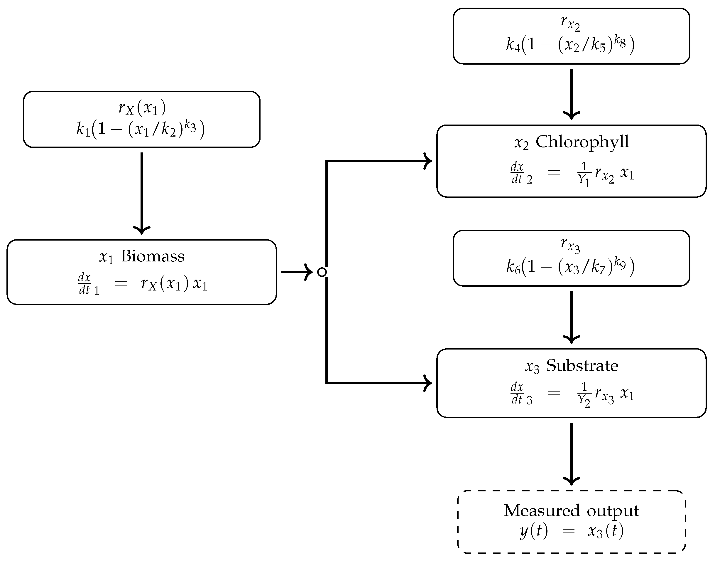
Biotechnological progress relies on accurate data analysis and resilient mathematical models. This section pertains to the analysis of data and the construction of a mathematical model for our inquiry regarding the growth of microalgae in a flat-plate photobioreactor. This technique converts unprocessed, empirical data into valuable observations, enhancing the understanding and refinement of microalgal cultivation. For this reason, in this work, the main parts of the dynamic model of the photobioreactor are proposed, and we model the dynamics of the biomass, chlorophyll and nutrients, as shown below.
To achieve accurate microalgal growth dynamics, the process shifts from data analysis to mathematical modeling. This model corresponds to the interactions and events witnessed in the conducted experiments. The dynamic model integrates growth factors and environmental conditions for thorough comprehension. The model predicts how microalgae behave in different scenarios to improve the design and functioning of photobioreactors. Validating the model with experimental data enhances its robustness and reliability, making it more applicable for future studies in microalgal biotechnology. Various factors interact to affect the growth and productivity of microalgae in photobioreactors. In [
52], the significance of culture conditions is emphasized, particularly in relation to chlorophyll content, while [
53] focuses on photosynthetic efficiency. Ref. [
54] shows and highlights the importance of photobioreactor design.
In the study of microalgal growth within photobioreactors, as explored in [
55], several key parameters are defined to model the growth kinetics:
, , and represent the concentrations of biomass, chlorophyll, and substrate, respectively.
, , and are rate constants specific to each growth process.
, , and denote saturation constants for biomass, chlorophyll, and substrate, respectively, indicating the concentration levels at which the growth rate starts to plateau.
, , and are exponents in the biomass growth equation, reflecting the nonlinear response of the growth rate to biomass concentration.
The Levenberg–Marquardt (LM) algorithm will be used as a nonlinear optimization method for curve fitting to determine the kinetic parameters of the system. This method was chosen because it combines the stability of gradient descent with the convergence speed of the Gauss–Newton method. The process involves minimizing the sum of the squares of the differences between the experimental data and the theoretical model by adjusting the damping factor
iteratively. This will result in robust values being obtained for the rate constants
and other parameters of interest, ensuring high statistical accuracy even in models with strong nonlinear dependence [
47].
In addition, their nominal values and admissible ranges were selected from well-established kinetic models reported in the microalgal and bioprocess literature. A reduced subset of sensitive parameters was then fine-tuned using the experimental batch data by minimizing the discrepancy between model predictions and measured profiles. This approach avoids overparameterization and ensures physical interpretability while providing a consistent basis for observer design and validation [
56].
These parameters and their interactions are crucial for understanding and optimizing microalgal growth in photobioreactors, providing insights into the efficiency of different growth conditions and the potential for scale-up in industrial applications.
3. Process Modeling for Biological Systems
Process modeling plays a role in the research of microalgae, allowing for the understanding of and enhancement in their growth and progress in diverse settings [
57]. These models are instrumental in simulating, designing and refining the cultivation of microalgae by factoring in elements like media composition, light exposure and temperature. They also take into consideration how light and temperature impact growth, decay, and biosynthesis processes as the physical characteristics of the culture medium [
58]. Nevertheless there is a necessity for models that are applicable to systems while considering the correlation between growth and salinity levels [
1]. In this study, the following equations represent the core of such modeling:
To make the observer design fully reproducible, we explicitly state the nonlinear state-space model used throughout this manuscript. We define the state vector as
The growth rate terms are nonlinear functions of the corresponding states:
Using (
6)–(
8), the photobioreactor dynamics are written component-wise as
Therefore, the compact nonlinear state-space form
corresponds to the nonlinear vector field
where
denotes known operating conditions (e.g., temperature, illumination, aeration) and/or parameters used during the experiment. In the present work, the dynamic evolution is captured by the nonlinear dependence on
x, as shown in (
13).
Regarding the measured output, the available online signal is the substrate/glucose concentration; hence
These equations are fundamental in capturing the dynamics of microalgal growth in photobioreactors, as they describe the rate of change of biomass, chlorophyll, and substrate concentrations over time. The parameters within these equations, such as
,
,
,
,
,
, and the
exponents, are crucial in defining the specific growth conditions and responses of the microalgae. In the sophisticated domain of microalgal growth modeling, particularly in state-space nonlinear systems, the concept of state variables becomes integral. These variables, denoted as
,
, and
, represent the concentrations of biomass, chlorophyll, and substrate, respectively. The evolution of these state variables over time is governed by a set of differential equations, collectively forming a state-space nonlinear system. This system can be succinctly expressed as:
Here,
represents the derivative of the state vector with respect to time, indicating the rate of change of the state variables. Based on the nonlinear state Equations (1)–(3), the vector field
can be explicitly written as
where
denotes the state vector, and
u collects the known operating conditions. Since the growth rate functions
,
, and
are smooth nonlinear functions, the resulting vector field
is smooth and locally Lipschitz continuous in the region of operation. Whit
and
are constant yield coefficients:
relates biomass growth to chlorophyll production, while
relates biomass growth to substrate consumption. These parameters represent conversion efficiencies and are assumed positive and constant.
The output mapping is given by
which is linear and therefore globally Lipschitz. The term
signifies the additive modeling error inherent in the system. The output vector
comprises the measured states, providing a link between the model and empirical observations. This framework of state-space modeling is pivotal in capturing the complex dynamics of microalgal growth, enabling the prediction and control of the system under varying conditions.
4. Observer Design
The concept of a observer is considered essential in system dynamics, particularly when studying biological systems like microalgal development. An observer deduces the internal state of a dynamic model by analyzing the system’s exterior outputs. This becomes especially crucial when some state variables of the system are not readily measurable or quantifiable. The design of the observer depends on the state-space representation of the system and its observability. Observability quantifies the degree to which external outputs may accurately predict the internal states of a system. This section offers a comprehensive explanation of the basic principles of observer design, focusing specifically on the linear observability criteria in state-space nonlinear systems. An analysis is conducted on the mathematical principles that underlie the method of local linearization, which is used to approximate equilibrium positions. In addition, the mechanism used to confirm observability is examined. Comprehending these principles is considered essential for understanding complex systems and using control approaches in both biological and technical fields.
4.1. Linear Observability Conditions
In the context of state-space nonlinear systems, the design of an observer is a critical aspect. Such systems can be represented as:
where
is the derivative of the state vector
over time, representing the evolution of state variables. The control input vector is denoted as
. The function
is a nonlinear, smooth vector function, Lipschitz continuous in
x and uniformly bounded in
. The term
represents the additive modeling error, and
is the vector of measured states.
The monitoring of photobioreactors aims to deliver actionable, real-time data regarding the culture and the process used to facilitate oversight, diagnosis, and regulation. In flat-panel photobioreactors, a limited array of signals is often accessible online at a cost-effective and reliable level for industrial applications. The exit substrate/glucose concentration can be continually measured with an online device, while operating variables like as temperature, pH, lighting level, and aeration/air flow are consistently documented. Nevertheless, essential biological metrics that directly measure process performance—particularly biomass concentration and chlorophyll content—are typically acquired through offline sampling and laboratory analyses, which are labor-intensive, pose contamination risks, and fail to deliver continuous data.
4.2. Proposed Nonlinear Observer
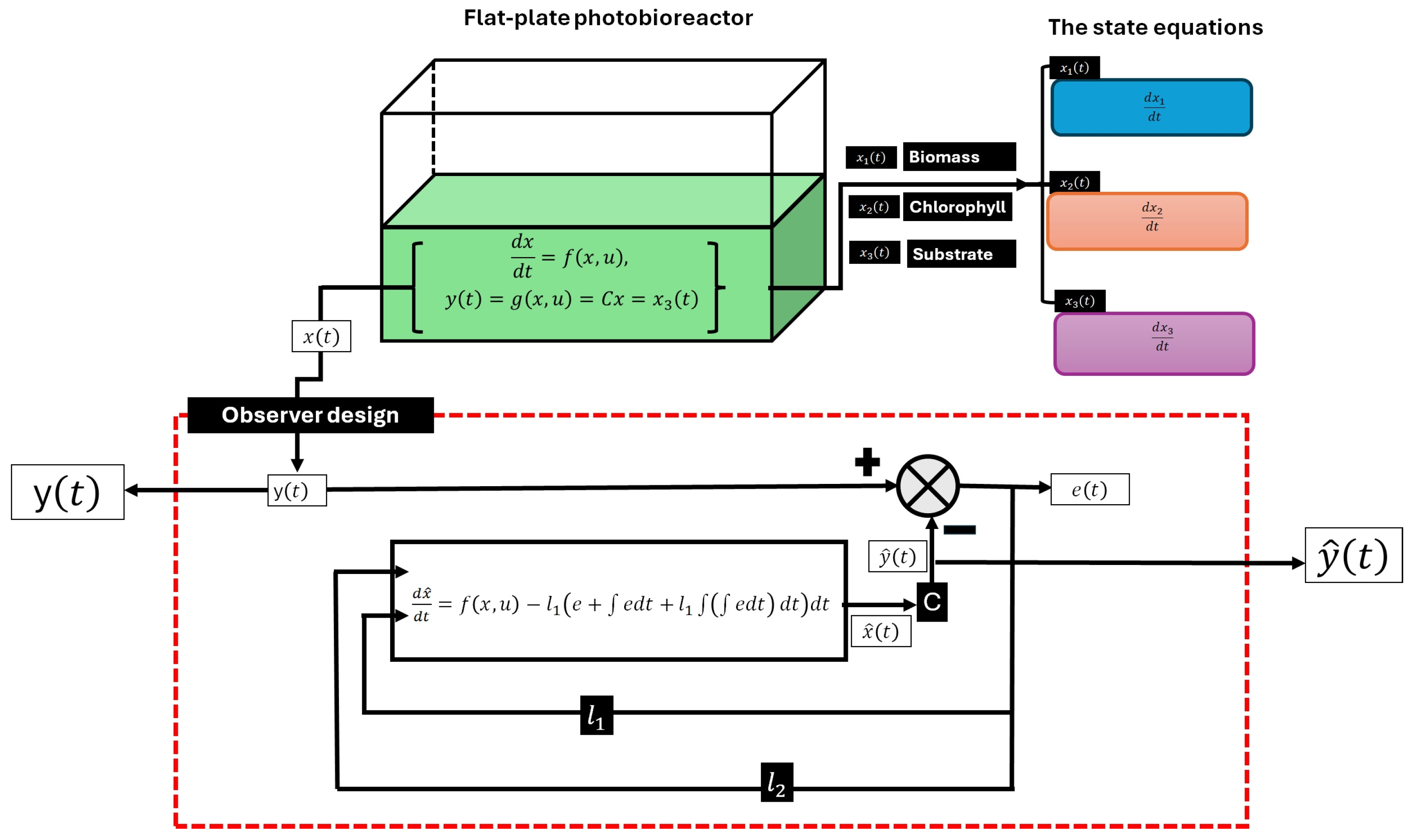
To address this constraint, we implement a model-based monitoring architecture wherein a nonlinear state observer functions as a virtual sensor. An experimentally validated nonlinear growth model is integrated with the measured output
(the online substrate/glucose measurement) and the known operating conditions/inputs
to reconstruct the internal state vector
, encompassing biomass and chlorophyll (as shown in
Figure 1). These online estimates provide ongoing productivity monitoring and prompt identification of atypical behavior (e.g., growth inhibition) while offering dependable input for sophisticated automation tactics without complicating instrumentation. Furthermore, due to the enduring uncertainties in bioprocess measurements and models (such as consistent sensor bias or drift and perpetual model discrepancies), the suggested nonlinear
observer integrates integral actions that augment disturbance rejection and bolster monitoring robustness in these practical scenarios.
Consider the nonlinear photobioreactor model
where
is the state vector,
collects known operating inputs/conditions, and
is the measured output. In this work,
corresponds to the available online measurement (substrate/glucose), and
C is the corresponding selection matrix.
Let
denote the state estimate,
, and define the output estimation error
The proposed nonlinear
observer (virtual sensor) is explicitly given by
where
are observer gain matrices of compatible dimensions. The additional integral actions enhance robustness against constant disturbances and persistent model mismatch (e.g., constant sensor bias/drift).
Local Linearization Around an Equilibrium Point:
An equilibrium point in this system is defined as a pair . To analyze the observability of the system, we consider its linear approximation near this equilibrium point.
Observability Tests:
The linear system representation can be expressed as:
where
is the state matrix,
is the input matrix,
is the output matrix, and
is the feedforward matrix. In a time-invariant system, these matrices are constant. The state vector
x is of dimension
n, the input vector
is of dimension
m, and the output vector
is of dimension
p. This framework allows for the assessment of the system’s observability, which is crucial for the effective design and implementation of an observer in the context of microalgal growth modeling and other biological systems.
The system, as represented in the above equation, is characterized by the following Jacobian matrices:
This process is referred to as the local linearization of (9) around the equilibrium point. In the context of observability tests in this work, system (9) is considered as unforced, that is, a homogeneous time-invariant system, which can be expressed as:
It is important to note that the linearization around the equilibrium point is employed solely for initialization and local stability analysis purposes. The observer implementation itself is fully dynamic and follows an iterative update scheme, where the state estimates are continuously updated in time using the original nonlinear model and the measurement error. Thus, the estimation process does not rely on a fixed linear approximation but evolves iteratively through the nonlinear observer dynamics.
For the observability tests, the focus is on whether the rank of the observability matrix,
O, equals
n, where
O is defined as:
The observability of the system at the equilibrium point is determined by the test matrix O. In the analysis of dynamic systems, the equilibrium point, denoted as , and the observability matrix, O, are defined as follows:
Table 1 summarizes the linearized state-space representation of the nonlinear photobioreactor model around a selected operating point. The matrices are obtained by evaluating the Jacobian of the nonlinear system at the equilibrium state
, which corresponds to the steady-state conditions reached during the experimental batch operation under constant input conditions. This equilibrium point is used as the nominal operating condition for observer initialization and local stability analysis.
The determinants and ranks of these matrices are calculated as:
For the purpose of assessing system observability, various configurations of
C are considered:
4.3. Analysis of Observer Stability Using Lyapunov’s Method
The observer’s mathematical model, incorporating a double integral, is represented as follows:
In this model, for all errors
, the dynamic behavior of the estimated variable
x is proposed to be:
Consequently, the error dynamics are expressed by:
Introducing
and
, the error equation is reformulated as:
Upon differentiating this equation twice, the third derivative of the error is obtained:
and this leads to the following differential equation for the error vector
E:
Here, , , and .
Note: For compactness, the observer error dynamics are expressed in vector–matrix form. Define the augmented error vector
, whose dynamics can be written as
A quadratic Lyapunov function is selected as
, where
is the symmetric positive definite solution of the Lyapunov equation
, with
.
To analyze the stability of the observer error dynamics, consider the quadratic Lyapunov function
where
is the symmetric positive definite solution of the Lyapunov equation
, with
.
Evaluating the time derivative of
along the estimation error trajectories yields
Therefore, under the condition
, the observer estimation error converges exponentially to zero.
This indicates that the system is asymptotically stable. The above utilization of Lyapunov’s method in the examination of the suggested nonlinear state observer model holds great significance. This approach offers a rigorous mathematical framework to guarantee the stability of the system, which is crucial when considering the growth of microalgae in photobioreactors. Lyapunov’s approach provides a broader and more encompassing view of stability compared to the difference method, which only offers insights into the local behavior of the system.
5. Numerical Results
As shown in
Figure 2, this section provides a detailed analysis of the results from the proposed model-based observer and compares the estimated states with the corresponding experimental measurements. This comparison is crucial for confirming the theoretical structure and assumptions introduced in the previous
Section 4.
The kinetic parameters
and
were identified from experimental batch data using nonlinear least-squares regression based on the Levenberg–Marquardt algorithm, as summarized in
Table 2. The reported uncertainty associated with each parameter corresponds to the standard deviation obtained during the optimization procedure.
Model adequacy was evaluated using the root mean square error (RMSE) and the coefficient of determination (), computed by comparing experimental measurements with model-predicted trajectories. The resulting values exceeded 0.94, indicating strong agreement between the model and the experimental observations.
These results demonstrate that the estimated parameters are statistically consistent with the experimental data, and that the residual fitting error remains within the expected variability inherent to biological systems.
Values are expressed as the mean ± standard deviation. Different letters within the same row indicate significant differences ().
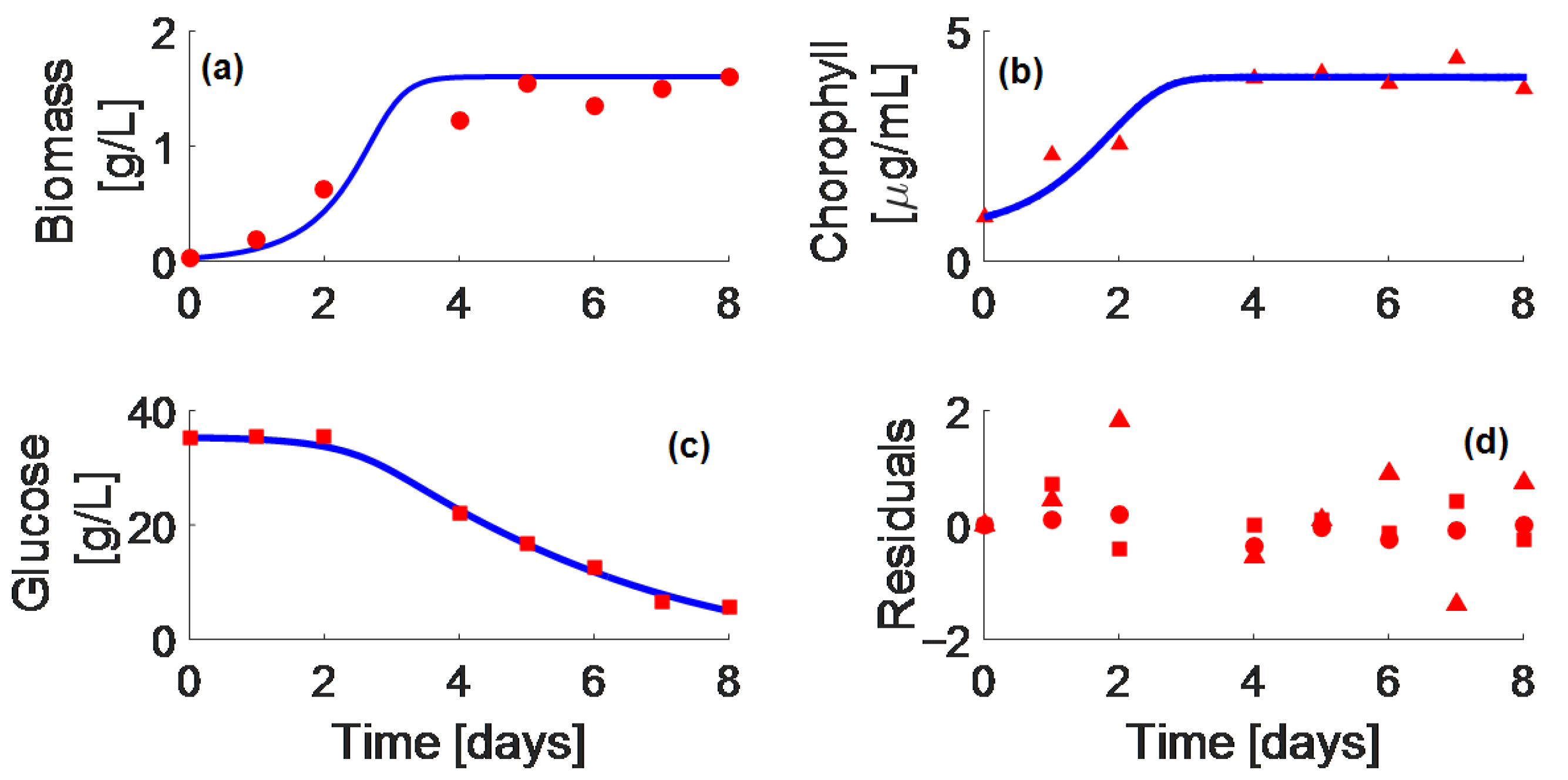
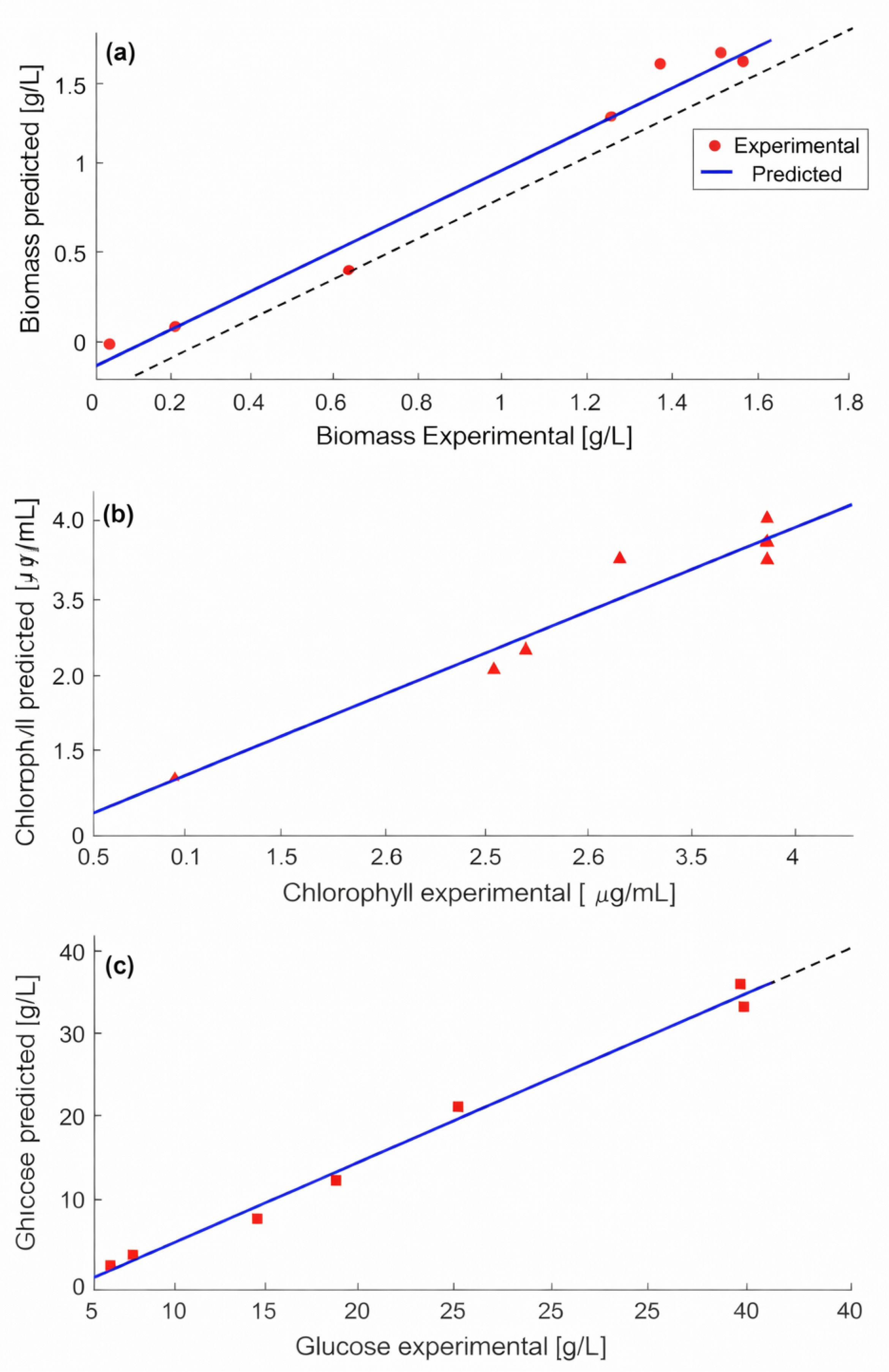
The experimental data was used to obtain the nine parameter values of the model developed. As demonstrated by the correlation coefficients in
Figure 3 and
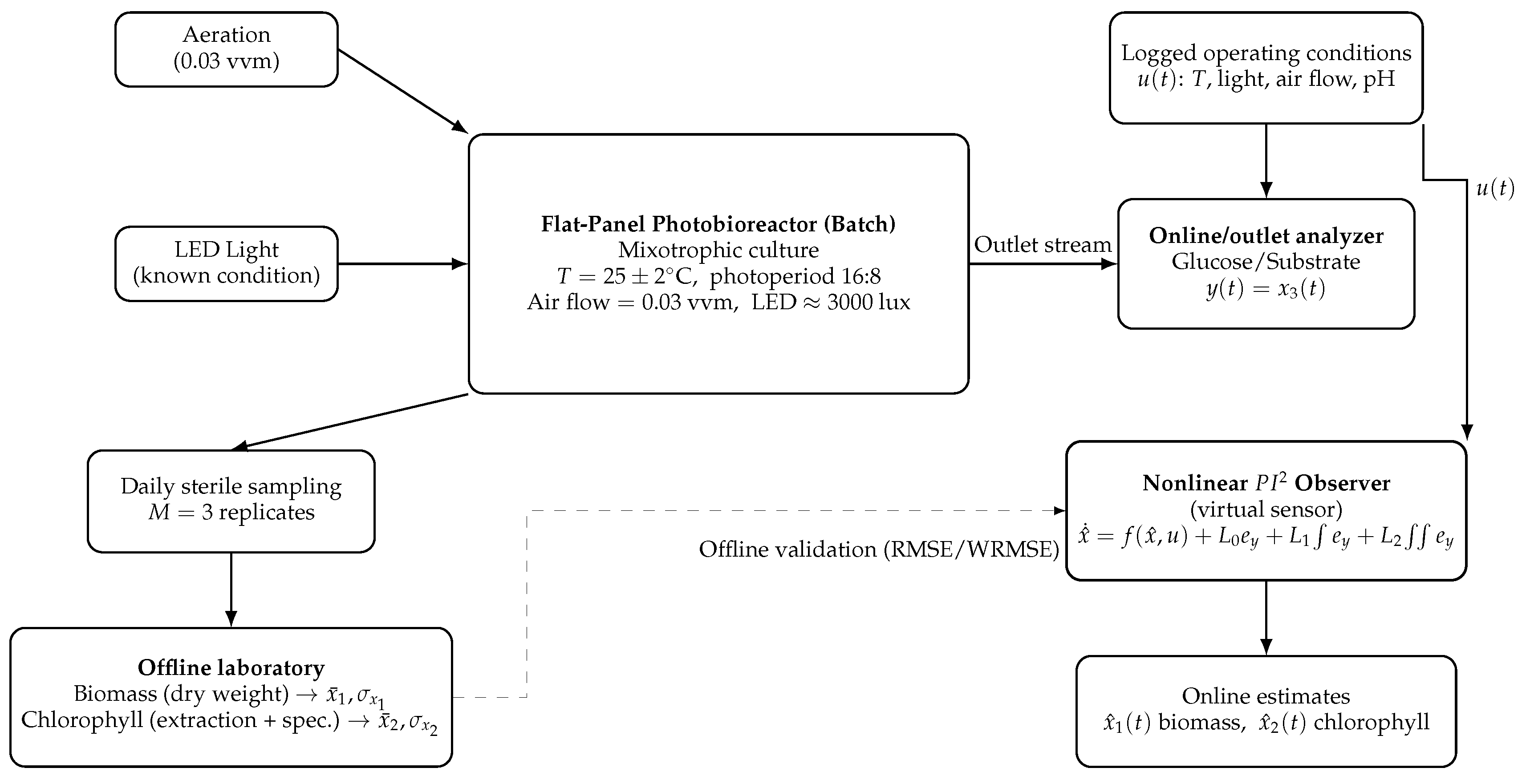
Figure 4, which are above 0.99, the parametric identification is illustrated. A simplified schematic of the experimental setup and the model-based monitoring framework is provided in
Figure 5 to clarify how the reported results relate to the physical photobioreactor. The diagram summarizes the main operating conditions and process streams, distinguishes the measured output used by the observer (online/outlet substrate measurement,
) from the offline laboratory measurements (biomass and chlorophyll), and illustrates how these data are integrated for parameter calibration and for validating the proposed nonlinear
observer against experimental profiles.
The parameter values obtained in the present study are disparate, which may be ascribed to the divergent operating conditions utilized in each case, i.e., disparate carbon sources, continuous or batch operation, temperature, and pH, among others. The numerical results reported here are based on the experimental batch dataset described in
Section 2. On each sampling day, biomass (dry weight method), chlorophyll (solvent extraction and spectrophotometry), and glucose/substrate (DNS method, outlet/online measurement) were quantified. All measurements were performed in
triplicate at each sampling instant (
). Thus, the experimental curves in
Figure 6,
Figure 7 and
Figure 8 correspond to the sample mean, and the associated dispersion is represented by the sample standard deviation. These experimental profiles were used both for parameter calibration/identification and for the offline validation of the proposed observer against the baseline observer.
The residuals depicted in
Figure 3d represent normalized instantaneous discrepancies between experimental measurements and model projections. The residuals are derived by normalizing the pointwise estimation error against the associated experimental variability, facilitating a direct comparison of biomass, chlorophyll, and glucose signals on a unified scale. The residuals are non-dimensional and offer insight into the temporal distribution and consistency of the model fitting error during the batch procedure.
The numerical results generated demonstrate the resilience and practicality of the observer model in real-life situations. The simulations were conducted with great attention to detail using MATLAB R2023a and Simulink R2023a (MathWorks, Natick, MA, USA) and the ‘ode45’ nummerical method to solve differential equations. Selecting this particular strategy guarantees a high level of precision and reliability in the simulation outcomes. Two out of three internal, non-measurable, nonlinear states were estimated in an online numerical experiment. Glucose concentration was measured in the photobioreactor output using an online device, with substrate and chlorophyll concentrations serving as estimate variables.
The numerical simulations and observer-based estimations were initialized using experimentally consistent initial conditions extracted from the first sampling day. Specifically, the initial biomass, chlorophyll, and substrate concentrations were set to , , and , respectively. These values correspond to the initial experimental measurements and were consistently used for the process model, the proposed observer, and the extended Luenberger observer, ensuring a fair and reproducible comparison.
The considered problem corresponds to a photobioreactor system for microalgal cultivation, where the model describes the interaction between biomass growth, chlorophyll dynamics, and substrate (glucose) consumption. All numerical simulations were performed using the complete nonlinear model, with initial conditions and saturation constants selected according to the experimental operating conditions.
Extended Luenberger Observer (Baseline)
For comparison purposes, an extended Luenberger observer (ELO) is implemented as a baseline estimator. The ELO is obtained by applying a local linearization of the nonlinear photobioreactor model around an operating point and injecting a linear correction term based on the output estimation error. Its structure is given by
where
is the estimated state vector,
is the measured output (substrate concentration),
, and
is the observer gain matrix.
In this work, the ELO gain was selected as
which ensures locally stable error dynamics around the equilibrium point while preserving a fair comparison with the proposed observer. No integral action is included in the ELO structure, making it sensitive to constant disturbances, parametric uncertainty, and modeling mismatch, which are intrinsic to biological processes.
The Lyapunov stability of the proposed nonlinear
observer is established in
Section 2.4 following standard nonlinear observer theory. Under the smoothness and boundedness assumptions on the vector field
, the estimation error dynamics are shown to be asymptotically stable using a quadratic Lyapunov function, in accordance with classical results in nonlinear systems theory [
59].
The results presented here are not just numerical outputs; they connect theoretical predictions with actual experimental data.
A simplified schematic of the experimental setup and the model-based monitoring framework is provided in
Figure 5 to clarify how the reported results relate to the physical photobioreactor. The diagram summarizes the main operating conditions and process streams, distinguishes the measured output used by the observer (online/outlet substrate measurement,
) from the offline laboratory measurements (biomass and chlorophyll), and illustrates how these data are integrated for parameter calibration and for validating the proposed nonlinear
observer against experimental profiles.
The study of chlorophyll concentration dynamics within the photobioreactor environment reveals crucial insights into the photosynthetic efficiency and health of microalgae. This research delves into the temporal patterns of chlorophyll concentration, correlating these patterns with various growth conditions and environmental factors. The nonlinear observer model, adept at capturing the intricate dynamics of microalgal growth, also extends its precision to the estimation of chlorophyll levels. This aspect of this study is particularly significant, as chlorophyll concentration is a key indicator of microalgal vitality and a determinant of biomass productivity.
Finally, it is important to take into account that the photobioreactor system may be affected by external disturbances, which can naturally arise in this type of application. These disturbances may be caused by a damaged sensor, poor electrical connections, or interference during sampling. Therefore, the simulation was carried out considering the case in which a perturbation is introduced in the
sensor, as described by:
By comparing the model’s predictions with real experimental data, a more profound understanding of the model’s effectiveness and limitations can be gained. This contrast is essential for emphasizing the practical significance of the observer model and showcasing its potential in real-world applications, as shown in
Figure 6,
Figure 7 and
Figure 8.
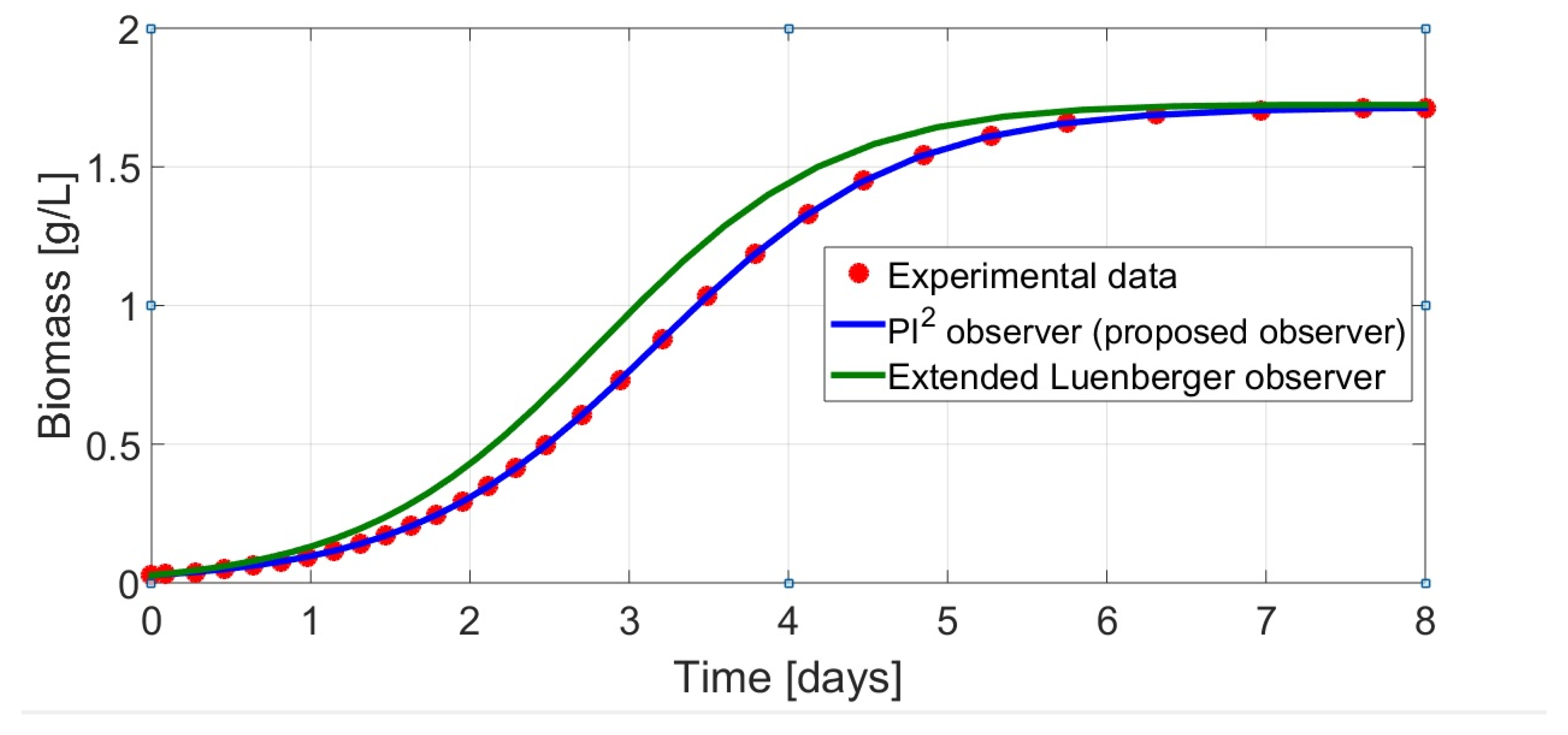
Figure 6 clearly and quantitatively demonstrates the superior performance of the proposed
observer compared to the extended Luenberger observer in biomass estimation, particularly with regard to estimation error. The
observer maintains a smooth and accurate fit to the offline experimental data throughout the entire growth curve. This results in minimal, stable estimation error, even during the complex exponential phase (days 2 to 4). This is due to its dual integral action, which provides superior adaptability and robustness when rejecting and canceling constant disturbances (e.g., sensor drift or constant modeling errors). In contrast, lacking this feature, the ELO exhibits persistent overestimation over the same period, leading to significantly larger estimation error. Consequently,
is obtained.
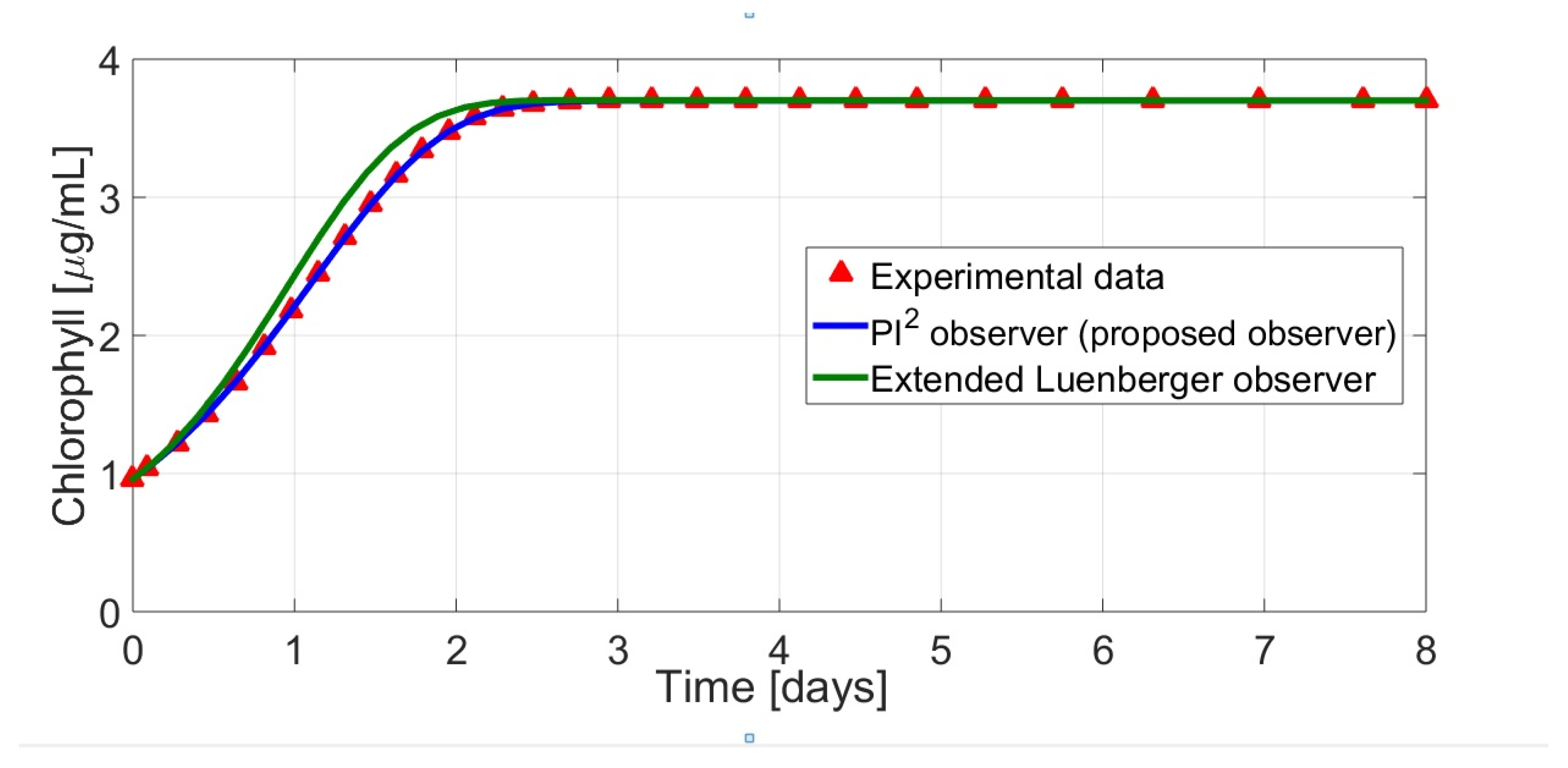
Figure 7 shows the estimated chlorophyll concentration, which, like the estimated biomass, reveals that the extended Luenberger observer significantly overestimates during the dynamic phase. This results in a root mean square error (RMSE) that is more than 14 times higher than that of the proposed observer,
. This substantial discrepancy in the estimation error suggests that the ELO is overly sensitive to the parametric uncertainties and modeling errors inherent in bioprocesses, which compromises its reliability. In contrast, the dual integral action of
allows it to effectively reject these disturbances, keeping the error close to zero. For industrial applications, the low estimation error of
is crucial as it ensures that automatic controllers receive accurate information in real time. This is fundamental for meeting quality standards and optimizing photobioreactor performance.
The proposed observer is a reliable tool for real-time industrial monitoring. It is important to note that biomass, representing the concentration of cells or microorganisms in a bioreactor, is a key state variable in industrial bioprocesses because it directly indicates the progress and productivity of the culture. However, directly and continuously measuring biomass in real time is often costly, slow, or impractical due to the need for manual sampling (which introduces contamination risk) or specialized online sensors. State observers, such as the analyzed here, offer a robust solution by providing an accurate virtual estimate of biomass based solely on readily available measurements (e.g., substrate consumption and/or chlorophyll-related signals).
WRMSE (proposed PI2 observer): WRMSE (extended Luenberger observer):
If experimental dispersion information is available (e.g., from triplicate measurements), the comparison can also be reported using the weighted RMSE (WRMSE).
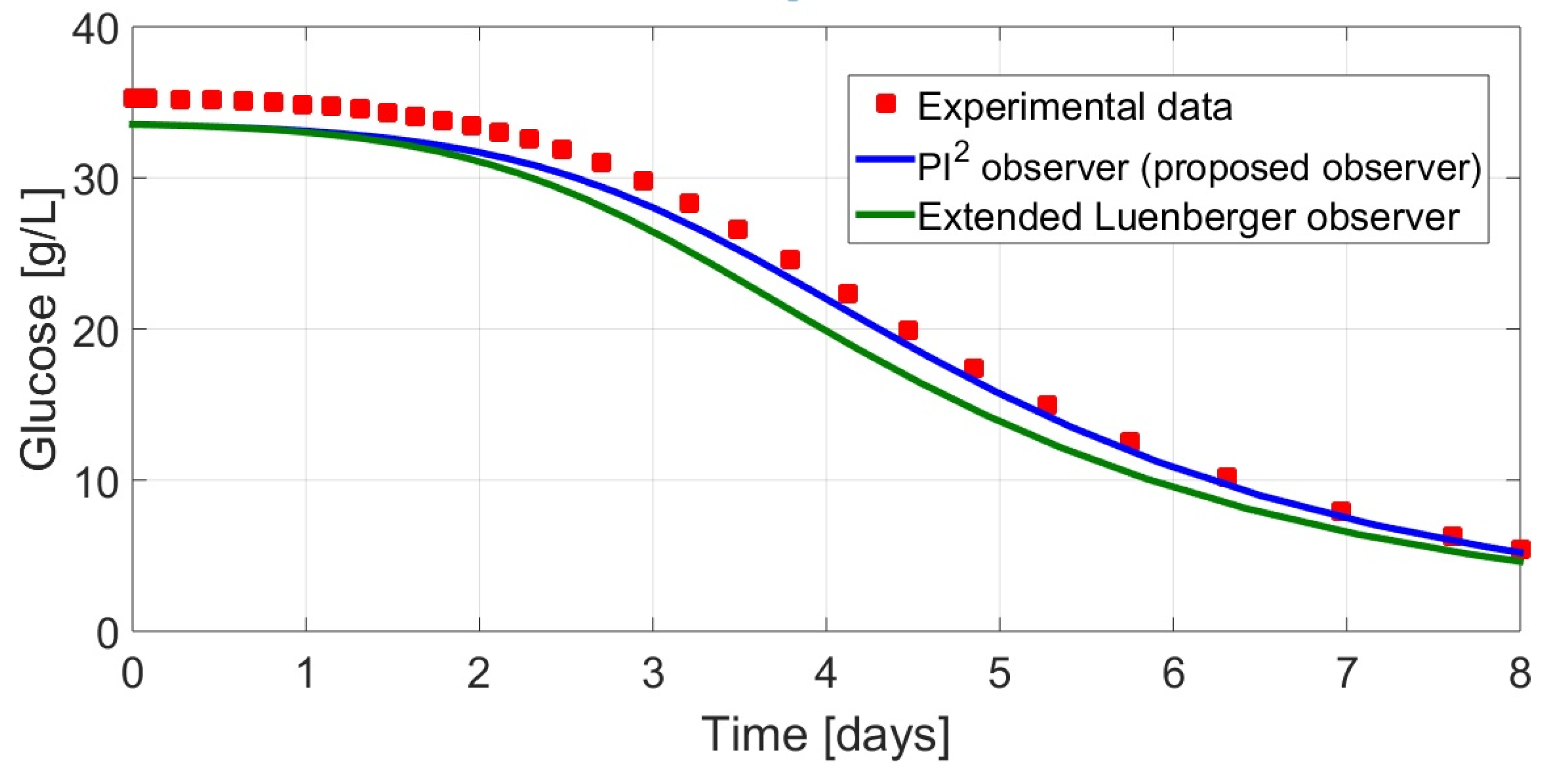
Regarding glucose consumption, the proposed observer provides a closer fit to the experimental profile over the full horizon, as reflected by the lower WRMSE. To complement this, the scalar WRMSE index depicts the time evolution of the absolute estimation error for glucose, showing that the proposed observer maintains a smaller error over most of the batch horizon, while the baseline exhibits larger deviations during the main consumption interval. Such differences are relevant for monitoring and decision-making (e.g., feeding strategies) in practical operation.
WRMSE (proposedPI2 observer): WRMSE (extended Luenberger observer):
The behavior of the estimation error, as evidenced by the WRMSE, shows that the Pi observer is the superior tool for tracking glucose consumption. The WRMSE value (approximately 0.0091) is more than eight times lower than that of the OLE (approximately 0.0760). The ELO’s consistent underestimation of glucose consumption (as can be seen in
Figure 5) results in a high WRMSE value, which poses an unacceptable risk in industrial control applications. This is because it would cause the system to believe that the substrate has been depleted faster than it actually has, which would compromise feeding decisions and consequently affect bioreactor productivity, as shown in
Figure 8.
It is noted that
Figure 6 depicts the absolute estimation error defined as
, whose magnitude is naturally observed at a smaller scale than the state trajectories shown in
Figure 5. Therefore, the different orders of magnitude in the vertical axes reflect the distinction between state values and estimation error, rather than an inconsistency in the results.
The extended Luenberger observer (ELO) is considered as a baseline approach and was implemented using standard gain selection based on local linearization around the nominal operating point. Unlike the proposed observer, the ELO does not incorporate integral action or uncertainty compensation, which makes it sensitive to model nonlinearities and parameter variations. Consequently, when experimental uncertainties and nonlinear effects are present, the ELO exhibits a larger estimation error, as observed in
Figure 6,
Figure 7 and
Figure 8.
The observer gains and model constants used for each estimation scheme are explicitly reported for completeness.
It is important to emphasize that the observer’s initial conditions are intentionally selected different;y from the experimental initial states. This is a standard practice in observer design, since the true initial state is assumed to be unknown. The objective is to evaluate the convergence capability of the observer under mismatched initial conditions. The initial discrepancy observed in
Figure 5 reflects the transient estimation error, while the subsequent convergence confirms the observability and robustness properties of the proposed observer.
The main benefits of the proposal are summarized below and discussed in greater detail below.
Superior Adaptability: The observer incorporates two integral terms, which guarantee accurate estimation and confer unique adaptability.
Perturbation Rejection: The observer demonstrates superior ability to reject unknown constant perturbations common in bioprocesses, such as sensor drift or persistent model errors.
Robust Self-Calibration: This adaptability is essential for effectively calibrating biological systems, ensuring stable performance even when faced with unmodeled variations and parametric uncertainties.
Consistent Accuracy: The experimental results confirm its reliability in state estimation, with significant performance improvements over conventional observers.



 ,
,