Abstract
The sports betting industry has been growing at a phenomenal rate and has many similarities to the financial market in that a payout is made contingent on an outcome of an event. Despite this, there has been little to no mathematical focus on the potential ruin of bookmakers. In this paper, the expected profit of a bookmaker and probability of multiple soccer matches are observed via Dirac notations and Feynman’s path calculations. Furthermore, we take the unforeseen circumstances into account by subjecting the betting process to more uncertainty. A perturbed betting process, set by modifying the conventional stochastic process, is handled to scale and manage this uncertainty.
1. Introduction
The gambling industry is a significantly large industry and has been growing its online presence consistently over the past years. The estimated amount of gross gambling revenue, being amount wagered less payouts, for online gambling businesses in UK and EU was around twenty-six billion euro during 2020 [1]. Around 40% of this is is generated from sports betting. The growth in online gambling is bound to continue as more markets are opening up since gambling licences are being generally viewed as a means to increase revenue for states [2]. It is therefore fairly straightforward to note that online sports betting is a multi-billion dollar industry.
Sports betting has therefore been a focus of interest in different academic circles with significant emphasis on problem gambling (for example [3,4]); profiling gamblers (for example [5,6]); the inefficient functioning of betting markets (for example [7,8,9]); or strategies to beat markets (for example [10,11]). In that respect, the focus has been on the clients of these services or the actual numbers/predictions generated by the services.
It would be expected that the solvency of a multi-billion dollar industry would also be of great interest to academics and regulators. Yet there has been scarce research on the solvency of the providers of this service, the sports betting companies themselves, with notable exceptions being [12,13]. Ref. [12] introduces a theoretical quantitative framework that can be used to measure the potential risk of a sports betting company from its trading operations by subdividing its portfolio of wagers into bundles according to their likelihood size. Ref. [13] is an in-depth overview and comparison of the perceived risks faced by banks and gambling companies ranging from compliance to operational risks.
The rationale for this vacuum in bookmaker solvency could be due to bookmakers being considered as the ‘bad’ guys that do not contribute to the welfare of society and the lack of systemic effects should a bookmaker fail. However, bookmakers are large corporations whose ruin, or inefficiencies, are bound to affect financial markets. The current state of affairs with respect to reserving is leading to an inefficient use of capital. Moreover, it would be ideal to have fair, stable, strong bookmakers that are able to enforce responsible gaming and limit access to money-laundering rather than bookmakers that are inefficient in their processes.
In this paper, we introduce the use of perturbed betting processes to determine bookmaker’s capital more accurately and the likelihood of ruin by taking example of a series of accumulators (also known as multiples) on soccer matches. The results can be extended to other sports or events—we used soccer as it is the most popular sport and one of the few sports in which three outcomes are possible due to the prevalence of draws.
In addition to traditional representations and calculations, the paper focuses on Dirac notations and Feynman’s path calculations in betting market scenarios. Although there is a vast literature on the use of these techniques applied in finance (see [14,15,16,17]), Dirac notations and Feyman’s path calculations are not commonly applied in insurance and betting industries. Utev and Tamturk applied them into actuarial risk and capital modeling [18,19]. In follow-up joint papers, the approach was used for insurance claim analysis [20], catastrophic modelling by combining epidemic and actuarial models [21] and stock market data analysis [22].
2. Bookmaker’s Expected Profit via Matrix Representation
A soccer match can end in one of three outcomes: home team win, draw and away team win. Let us assume that the probabilities for each one of these three outcomes are , and . However, bookmakers would use inflated probabilities when determining odds in order to guarantee a profit. We use standard notation as described in [11,23] to define implied probabilities a for and .
European odds are defined by . Let be the total value in units of wagers placed on outcome i. By all definitions, in terms of betting company, the revenue is and expected payout is . Hence, the profit of the company can be defined simply for a single match by
When n soccer matches are considered, we have different scenarios (tickets) because there are 3 options in a match as home team win, draw and away team win as seen in Figure 1.
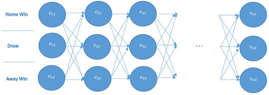
Figure 1.
Possible paths for n matches.
The betting of one stake based on multiple outcomes is called a multiple or an accumulator. Accumulators allow bettors to place one small stake to potentially large returns but exponentially low likelihoods. Bettors can put money on different options for n matches under assumption that they bet with n matches. By default, the expected profit for n matches is defined by
where is probability of being n independent events, so for Notice that
Similarly, representing multiply of n European odds on each match, and for
By default,
Bettors do not have to select to bet on every match. If the total number of matches is n, bettors can create tickets by selecting or 1 matches as desired, so the total number of options is
In this circumstance, the formula of the expected capital of betting company can be modified by
The company is expected to profit if while negative values of k can cause ruin of the company [12]. However, the optimisation of plays a vital role in terms of profitability of the company. In the case of a variable , the formula in (4) can be modified as
We assume that the bookmaker has data to compute of and can control by k. Even though is computable based on historical data, error term in the computation can produce surprising results.
As mentioned before, let be the total value in units of wagers for outcome i. Then, matrix of wagers values
Let and be a probability matrix and European odds matrix respectively for ith match. Then, probability matrix P for n matches is defined via tensor product
Similarly,
One can note that P and E are dimensional matrices. Expected profit of the betting company is shown via a trace function representing sum of the diagonal elements of .
3. Taking More Uncertainty into Account
In betting modeling, analysis of historical data does not reflect current situation perfectly. For example; referee mistakes [24], weather on the day of the match [25], distance travelled to match [26] and injuries of players can directly affect the outcome of the match. Therefore, even if a precise prediction is made, we need to modify the stochastic process with random uncertainty to make more realistic. This issue will be discussed more comprehensively in Section 5.
As mentioned before, for the ith match, probability of home win is , probability of draw is and probability of away win is . Let be probabilities of unpredictable things, and
are modified probabilities by
as
where we assume that and for . Under these conditions, the corresponding matrix for the ith match can be written as
Modified probabilities for n matches can be shown in the following matrix via tensor operator
According to and random variables, we can obtain different results, and get the average value by using simulation methods like Monte Carlo.
where M is a big enough number.
Notice that even if we modified P, E was not exposed to change because E is only computed by historical data while based on historical data analysis and unpredictable things in recent time.
4. Bookmaker’s Profit via Path Calculation
The path calculation approach has been applied to many different disciplines. To apply the path calculation approach in gaming, we have to think of the outcome of each match as a location or value at a different time. For example, let us consider five betting tickets for four matches as per the Table 1 below.

Table 1.
Betting Tickets.
In this table, represent home win, draw and away win, respectively. Now, we can consider the betting process via path calculation as per Figure 2. For example, the first ticket assumed the home teams will win the first and third matches, the away team will win the second match, and the last match will end in a draw. To make the our approach more clear, the betting process can be imagined as a time series by considering the matches as time, and results as locations or values.
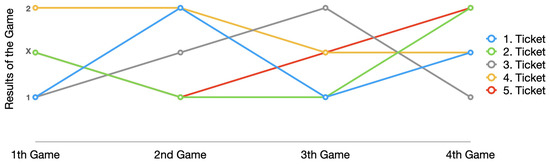
Figure 2.
Path representation of Betting.
Between two spacetime points at time and at time , the propagator of the quantum system can be defined as the probability transition amplitude via the wavefunction [27]
where K is called as Feynman kernel. By using Hamiltonian operator with bra-ket notations, the propagator can be written as
In other words, a propagator makes the state function at spacetime point move to another spacetime point .
Dirac defined notations about vectors in Hilbert space that corresponds to a physical system [28]. In Dirac formalism, and represent column and row vectors, which are used to show quantum states. A bra is the Hermitian conjugate transpose of the corresponding ket. Elements of or consist of 1 in position i and 0 elsewhere on computational basis. Surely, a ket can be defined in different ways (e.g., Hadamard and Circular basis [29]). A quantum operator like represents a matrix
In the propagator in (6), is an operator in semigroup form with Hamiltonian operator H. In physics, the Hamiltonian of a system is defined as the sum of kinetics and potential energies [28],
where K and V are representing kinetic and potential energy of the system respectively.
Furthermore, Hamitonian operators provide a way to go to quantum formalism from a classical Markovian approach, which is characterized by the continuous semigroup with generator Q. By taking minus generator operator equal to the corresponding Hamiltonian , we have . In general, the Hamiltonian operator H does not need to be a generator, specifically for the cases of non-embeddable Markov chains [18].
Throughout the quantum parts of this paper, we work on a Hilbert Space that is a complete vector space. Regardless of finite or infinite dimensional, a Hilbert space is separable if its basis is countable [28].
The scalar product of the basis states and is known as Dirac-delta function, and with the Fourier representation, it is written by [14]
where is momentum space basis with the completeness equation . Inner products of basis state and momentum basis state are
where is the eigenstate of the momentum operator (e.g., let P be a momontum operator, so ).
For actuarial random walks, the following propagator has been computed by Tamturk and Utev in the previous papers [18,19] and follow-up joint papers [20,21] with respect to several Hamiltonian operators with the help of the completeness equation and corresponding eigenvectors of different Hamiltonian operators,
where and are eigenvalue and eigenvector of the Hamiltonian operator, i is complex unit.
4.1. Transition Probability via Path Calculation
Regarding the path calculations, the main difference between gambling and the other disciplines is that order of the games does not change the results. Let us consider the following propagator with a matrix operator by assuming that is location (result) of i-th match as
Notice that all rows are taken as the same since we assume that the location of the th match is independent from the ith match. Sum of probabilities of the all the possible paths can be showed by
For the sake of simplicity, let us assume denoted by because
where and . Note that this statement is not true for diagonal operators .
4.2. Hamiltonian Operator for Expected Profit
If an operator is self-adjoint (adjoint-operator is equal to itself), it can be called as Hermitian operator [28]. A Hermitian Hamiltonian matrix can be diagonalised with help of the following transformation
where U is a unitary matrix. If U is a square matrix, and . Elements of D are eigenvalues representing energy levels.
where U is a unitary matrix, is its adjoint. Similarly, and can be written in the following forms:
and
Then,
where is unitary matrix.
Hamiltonian operator can be defined for the ith match by
However, cannot be generalized for multimatches case by
because does not give the total wage amount for each possible result; so instead of that, the dimensional W matrix mentioned in Section 2 is taken into account.
where V is unitary matrix, and the diagonal elements can be computed as
Regarding finding the expected profit and capital of the betting company, we will use Hamiltonian operators and for transition probabilities and corresponding odds. Now let us find probability of a single match via the transformation in Equation (7).
where the main complication is finding the eigenvalues of the Hamiltonian operators.
For a single match, we defined as
where it can be noticed that we added inside of to set up an independence between and .
When is substituted into Equation (9), we will obtain
For n matches, probability of n events via path approach,
can be computed by multiplying n integrals which will cause the long computation time, so for the sake of simplicity, we consider for the n events, and define new for n matches as
where and .
Similarly, the odds for n matches can be computed by following path approach with Hamiltonian operator
In this circumstance, the expected profit is
where is diagonal element of W.
Example 1.
Let us assume the probabilities of three matches are as in Table 2, and let us calculate probability of being draw for the first match, away win for the second match and home win for the third match.
Table 2.
Probabilities of three matches in Premier League.
In this circumstance, for draw, away win and home win, respectively,
Then,
With P and , the probability of respectively for the three matches is found by
Similarly,
The profit of the betting company can be computed as
4.3. Ruin Probability of the Betting Company
Let , be numbers of the matches in the i-th week. Then, ruin probability of the company at the end of the m weeks with assumption of 0 initial reserve can be computed by
where T is the ruin time defined by
As seen from the ruin formula in (14), we consider weekly capital of the company as integer values—this can be done by truncated numerical approach. However, finding the probability of the capital is based on complex computations for large time scale and high number of matches. Another challenge in terms of the computation is dynamic odds. We refer this to future researches.
5. Perturbation of Betting Process
Classical Markov processes may be perturbed to produce new Markov chain with similar statistical properties [30,31]. Perturbation of Markov process is quite an important approach in order to take unpredictable things into account. Therefore, the logic is simply based on modification of the random process without changing the general properties.
In continuous time, the transition matrix can be found via the generator matrix.
where Q is called the generator of the continuous time Markov process
The sum of the elements in each row of Q is zero with
where
For the small ,
As mentioned in Section 4, , so the stochastic process can be perturbed by modifying the generator matrix. For example, let us consider generator matrix on
Then, as mentioned in Feigin and Rubinstein’s article [30], perturbed generator can be found by
where R is a replacement matrix. With different versions of the replacement function, we can modify the stochastic process in various ways. However, we follow a different way. As mentioned in Section 4, Hamiltonian operator H does not need to be , which us gives more flexibility. The perturbed Hamiltonian operator can be defined by
where V is a Hermitian operator. For the ith match, the probabilities of the changes caused unpredictable situations is displayed by
where and represent the unpredictable part for i-th game. By default, + . Furthermore, more restrictions can be added like for and . However, this is not a research interest for us at this stage.
The total change for n matches via tensor product is
In this circumstance, the profit of the company after the n matches is
The equation above can be computed with respect to different Hamiltonian operators. This gives us a flexibility to play on. Of course, the perturbed process can be defined in more complex ways by taking seasonal weather situation, pandemic and macro economic variables, etc. into account in further research.
6. Conclusions
The betting sector is growing in a phenomenal rate, especially in the US [2], and notwithstanding the size of the industry, quantitative developments have focused on getting accurate odds or profiling customers. There is little to no work on the potential ruin of a bookmaker. Moreover there is a huge gap between the few theoretical approaches and applications in the betting sector.
In this paper, the betting process has been considered as a time series to apply the path approach with Dirac notations. We think that this kind of new approach will attract the interest of researchers in other disciplines to this sector, and more collaborative work will be produced in interdisciplinary work environments.
Furthermore, the application of such techniques can help in comparing the performance and comparative risk of different bookmakers, which could be used to better manage the financial performance of a company. Currently, the gambling market is in a phase of mergers and acquisitions at a valuation of more than one billion dollars per activity (example [32,33]). The application of more complex techniques such as those presented here could provide a relative edge when considering larger trades.
Author Contributions
Conceptualization, D.C. and M.T.; methodology, D.C. and M.T.; writing, D.C. and M.T.; visualization, D.C. and M.T.; supervision, D.C. and M.T.; project administration, D.C. and M.T. All authors have read and agreed to the published version of the manuscript.
Funding
This research received no external funding.
Institutional Review Board Statement
Not applicable.
Informed Consent Statement
Not applicable.
Data Availability Statement
Not applicable.
Acknowledgments
We thank AppliedMath editors for the APC waiver, and Sergey Utev (University of Leicester) because we were inspired by his previous articles about path calculation with quantum mechanics.
Conflicts of Interest
The authors declare no conflict of interest.
References
- European Gambling and Betting Association. European Online Gambling: Key Figures 2020 Edition. 2020. Available online: https://www.egba.eu/uploads/2020/12/European-Online-Gambling-Key-Figures-2020-Edition.pdf (accessed on 30 December 2021).
- Hancock, A.; German, S. Paying for the Pandemic: US Politicians Gamble on Sports Betting. The Financial Times. Available online: https://www.ft.com/content/bb04b14c-e215-4ae8-a655-2bf85fcb73c0 (accessed on 31 April 2021).
- Buhagiar, R.; Cortis, D.; Newall, P.W.S. Why do some soccer bettors lose more money than others? J. Behav. Exp. Financ. 2018, 18, 85–96. [Google Scholar] [CrossRef]
- Newall, P.W.S. Dark Nudges in Gambling. Addict. Res. Theory 2018, 27, 65–67. [Google Scholar] [CrossRef]
- Bezzina, F.; Sammut, D. The Online Poker Consumer: Investigating Personality Traits, Motives, and Demographic Characteristics. Int. J. Cust. Relatsh. Mark. Manag. (IJCRMM) 2012, 3, 55–73. [Google Scholar] [CrossRef]
- Hing, N.; Breen, H. Profiling lady luck: An empirical study of gambling and problem gambling amongst female club members. J. Gambl. Stud. 2001, 17, 47–69. [Google Scholar] [CrossRef] [PubMed]
- Axén, G.; Cortis, D. Hedging on betting markets. Risks 2020, 8, 88. [Google Scholar] [CrossRef]
- Hausch, D.B.; Ziemba, W.T.; Rubinstein, M. Efficiency of the market for racetrack betting. Manag. Sci. 1981, 27, 1435–1452. [Google Scholar] [CrossRef]
- Stark, D.; Cortis, D. Balancing the book: Is it necessary and sufficient? J. Gambl. Bus. Econ. 2017, 11, 1–6. [Google Scholar] [CrossRef]
- Candila, V.; Palazzo, L. Neural networks and betting strategies for tennis. Risks 2020, 8, 68. [Google Scholar] [CrossRef]
- Cortis, D.; Hales, S.; Bezzina, F. Profiting on inefficiencies in betting derivative markets: The case of UEFA Euro 2012. J. Gambl. Bus. Econ. 2013, 7, 39–51. [Google Scholar] [CrossRef]
- Cortis, D. On developing a solvency framework for bookmakers. Var. Adv. Sci. Risk 2019, 12, 214–225. [Google Scholar]
- Cortis, D.; Spiteri, L. iGaming versus Banking: Differences and Similarities. J. Gambl. Bus. Econ. 2021, 14, 15–31. [Google Scholar]
- Baaquie, B.E. Interest Rates and Coupon Bonds in Quantum Finance; Cambridge University Press: Cambridge, UK, 2009. [Google Scholar]
- Baaquie, B.E. IQuantum Finance: Path Integrals and Hamiltonians for Options and Interest Rates; Cambridge University Press: Cambridge, UK, 2007. [Google Scholar]
- Parthasarathy, K.R. An Introduction to Quantum Stochastic Calculus; Springer Science & Business Media: Basel, Switzerland, 1992; Volume 85. [Google Scholar]
- Lee, R.S. An Overview of Quantum Finance Models; Springer: Singapore, 2020. [Google Scholar]
- Tamturk, M.; Utev, S. Ruin probability via quantum mechanics approach. Insur. Math. Econ. 2018, 79, 69–74. [Google Scholar] [CrossRef]
- Tamturk, M.; Utev, S. Optimal reinsurance via Dirac-Feynman approach. Methodol. Comput. Appl. Probab. 2019, 21, 647–659. [Google Scholar] [CrossRef]
- Lefevre, C.; Loisel, S.; Tamturk, M.; Utev, S. A quantum-type approach to non-life insurance risk modelling. Risks 2018, 6, 99. [Google Scholar] [CrossRef]
- Tamturk, M.; Cortis, D.; Farrell, M. Examining the Effects of Gradual Catastrophes on Capital Modelling and the Solvency of Insurers: The Case of COVID-19. Risks 2020, 8, 132. [Google Scholar] [CrossRef]
- Hao, W.; Lefèvre, C.; Tamturk, M.; Utev, S. Quantum option pricing and data analysis. Quant. Financ. Econ. 2019, 3, 490–507. [Google Scholar] [CrossRef]
- Cortis, D. Expected values and variances in bookmaker payouts: A theoretical approach towards setting limits on odds. J. Predict. Mark. 2015, 9, 1–14. [Google Scholar] [CrossRef]
- Buraimo, B.; Forrest, D.; Simmons, R. The 12th man?: Refereeing bias in English and German soccer. Stat. Soc. Ser. 2010, 173, 431–449. [Google Scholar] [CrossRef]
- Iskandaryan, D.; Ramos, F.; Asarias Palinggi, D.; Trilles, D. The Effect of Weather in Soccer Results: An Approach Using Machine Learning Techniques. Appl. Sci. 2020, 10, 6750. [Google Scholar] [CrossRef]
- Goumas, C. Home advantage in Australian Soccer. J. Sci. Med. Sport 2014, 17, 119–123. [Google Scholar] [CrossRef] [PubMed]
- Perepelitsa, D.V. Path Integrals in Quantum Mechanics. Available online: http://web.mit.edu/dvp/www/Work/8.06/dvp-8.06-paper.pdf (accessed on 30 March 2022).
- Chang, K.L. Mathematical Structures of Quantum Mechanics; World Scientific Publishing Company: Singapore, 2011. [Google Scholar]
- Sutor, R.S. Dancing with Qubits: How Quantum Computing Works and How It Can Change the World; Packt Publishing Ltd.: Birmingham, UK, 2019. [Google Scholar]
- Feigin, P.D.; Rubinstein, E. Equivalent descriptions of perturbed Markov processes. Stoch. Process. Their Appl. 1979, 9, 261–272. [Google Scholar] [CrossRef]
- Leviatan, T. Perturbations of Markov processes. J. Funct. Anal. 1972, 10, 309–325. [Google Scholar] [CrossRef][Green Version]
- DraftKings. DraftKings Reaches Agreement to Acquire Golden Nugget Online Gaming in an All-Stock Transaction. Available online: https://www.draftkings.com/about/news/2021/08/draftkings-reaches-agreement-to-acquire-golden-nugget-online-gaming-in-an-all-stock-transaction (accessed on 12 March 2022).
- Yakowicz, W. Penn National to Acquire Score Media And Gaming For $2 Billion. Forbes. Available online: https://www.forbes.com/sites/willyakowicz/2021/08/05/penn-national-to-acquire-score-media-and-gaming-for-2-billion/ (accessed on 12 March 2022).
Publisher’s Note: MDPI stays neutral with regard to jurisdictional claims in published maps and institutional affiliations. |
© 2022 by the authors. Licensee MDPI, Basel, Switzerland. This article is an open access article distributed under the terms and conditions of the Creative Commons Attribution (CC BY) license (https://creativecommons.org/licenses/by/4.0/).