Article

Canonical Spectral Transformation for Raman Spectra Enables High Accuracy AI Identification of Marine Microplastics

by
Oscar Ramsés Ruiz-Varela
1,2,*,
José Juan García-Sánchez
3,
Roberto Narro-García
1,
Claudia Georgina Nava-Dino
1,
Juan Pablo Flores-De los Ríos
1,2,
Luis Fernando Gaxiola-Orduño
1,
Alain Manzo-Martínez
1 and
María Cristina Maldonado-Orozco
1,*
1
Faculty of Engineering, University Autonomous of Chihuahua, Circuito Número I s/n, Nuevo Campus Universitario, Nte. 2, Chihuahua C.P. 31125, Mexico
2
Technological Institute of Chihuahua, Avenida Tecnológico 2909, Chihuahua C.P. 31200, Mexico
3
Technological Institute of Higher Studies of Jocotitlán, Carretera Toluca-Atlacomulco km 44.8, Ejido de San Juan y San Agustin, Jocotitlán C.P. 50700, Mexico
*
Authors to whom correspondence should be addressed.
Microplastics 2026, 5(2), 71; https://doi.org/10.3390/microplastics5020071
Submission received: 17 January 2026 / Revised: 10 February 2026 / Accepted: 28 March 2026 / Published: 13 April 2026
(This article belongs to the Collection Feature Papers in Microplastics)

Abstract

The growing accumulation of microplastics in marine environments demands fast and accurate analytical methods for polymer identification. This study presents a new canonical spectral transformation (CST) strategy designed to extract the most relevant information of Raman spectra and enhance the performance of artificial intelligence (AI) models in the classification of microplastics. Using the Marine Plastic Database (MPDB) as the source of Raman spectra, five supervised models—k-Nearest Neighbor (KNN), Random Forest (RF), Extreme Gradient Boosting (XGBoost), Multilayer Perceptron (MLP), and a one-dimensional Convolutional Neural Network (CNN-1D)—were trained and evaluated under both typical (conventional methodology) and CST workflows using 500 noisy samples per category. The CST consists of representing a Raman spectra in a vector where only the magnitude peaks of the most relevant frequency bands of the spectra are retained and the remaining values are null. This CST minimizes the inclusion of non-target data reaching the AI models. All models achieved higher accuracy with CST, where CNN-1D achieved the most significant performance, increasing accuracy to 0.90. In addition, CNN-1D identified Polystyrene (PS) and Poly(methyl methacrylate) (PMMA) with a score of 100% and 99%, respectively. The results demonstrate that CST effectively enhances spectral feature extraction and can be generalized to other spectroscopic techniques, providing a scalable framework for AI-assisted microplastic identification in seawater samples.

1. Introduction

Plastic is a material composed primarily of high molecular weight polymers, long chains of repeating monomer units, as established by ISO/TR 21960:2020 [1]. To improve their properties, plastics use additives that modify their durability, flexibility, heat resistance, and even aesthetic qualities [2]. However, global use and the lack of efficient mechanisms for their disposal have led plastics to give rise to microplastics (MPs), defined as particles of 5 mm or less (ISO/TR 21960:2020) in lakes, rivers, seas, and oceans. These particles are the result of the degradation of larger plastics through physical, thermal, photochemical, and biological processes. Geyer et al. (2017) notes that the use of MPs has grown exponentially since the 1950s, starting with 2 million tons per year, and by 2015 the amount had increased to 380 million tons per year [3]. On the other hand, Hassan et al. (2024) mention that global plastic production is expected to reach 1800 million tons by 2050, raising significant environmental concerns [4].
The presence of MPs has been found In various ecosystems, soils, oceans, drinking water, and even in the human body, such as in blood [5], placentas [6], and breast milk [7]. The routes of entry include ingestion, inhalation, and dermal contact. The most common types of MPs are polyethylene (PE), polypropylene (PP), epoxy resin, and polyvinyl chloride (PVC), among others [8]. The most vulnerable ecosystems are aquatic ones, as bodies of water act as the main sink for MPs pollution. Therefore, wild marine fauna face the highest environmental risk from MPs pollution [9]. This pollution largely originates from wastewater treatment plant waste and the breakdown of larger plastics [10,11].
The ecological consequences are serious for all marine species. Tissues of marine organisms show contamination by MPs in about 70% of them across 64 aquatic environments [11,12]. MPs have been identified in more than 150 species of freshwater and saltwater fish [9,13]. These MPs pose a high risk throughout the food chain, including humans. In general, exposure to MPs has been linked to reproductive difficulties in animals, with a reported 41% reduction in reproduction among contaminated populations [10,14].
The accurate identification of microplastics is essential for assessing environmental impact. Raman Spectroscopy (RS) is a vibrational technique that offers a non-destructive method for characterizing MPs based on their molecular vibrations. However, spectra from field samples often differ from those of pure substances due to aging, contamination, and noise. Furthermore, Rocha-Santos et al. (2015) highlights the importance of preserving MP samples and avoiding their destruction, with the aim of being able to use them in different characterization techniques that support the relevance of research on the topic of environmental pollution [15]. It is well known that the use of optical microscopes, specifically stereoscopes, is the most commonly used instrument for an initial characterization of MPs [16]. However, RS offers a significant advantage in its ability to detect objects as small as 1 µm compared to 24 µm with Fourier-Transform Infrared (FTIR), another popular vibrational technique [17]. Nonetheless, it points out that RS cannot be applied to biological samples because of weak response and induced damage, but point out that RS has better spatial resolution and the potential to detect signals at higher frequencies [18,19].
On the other hand, manual spectral analysis by experts is possible but time-consuming and subjective. Automation using artificial intelligence (AI) provides a scalable and precise alternative. Recent studies have used AI models—such as Support Vector Machines (SVM), RF, CNN—to classify MPs using Raman spectra [20]. Usually, filtering, normalization, and category balancing are applied for the proper training of AI models.
Several authors have investigated model training using different preprocessing techniques, varying their methodology and the size of their datasets. This is the case of Fornasaro et al. (2020) [20], who standardized SERS-based procedures using 3650 samples for chemical detection with different Raman devices, while Lei et al. (2022) [21] addressed spectrometer variability through data augmentation, generating 4520 synthetic spectra from 108 original spectra of PE, PVC, PMMA, PP, among others [21,22]. Another methodology is dimensionality reduction, such as subsampling and Principal Component Analysis (PCA), which have been shown to be effective in improving signal clarity and model performance.
Feature selection (FS) focuses on extracting the most relevant information from the source or original spectra. Additionally, once the features are selected, it is only necessary to calculate or collect them in a new spectra [23]. In fact, this selection helps to analyze the data, reduce computational requirements, and improve the performance of the AI model [24]. In other words, FS is used to clean noisy, redundant, and non-target data [25].
In other studies, Rytelewska et al. (2022) highlight challenges such as autofluorescence and background noise in the identification of PE in samples from Polish water bodies, both of which are factors that impair model performance [24]. On the other hand, spectral features, such as the vibrational modes of carbon-oxygen double bonds (C=O) at 1643 cm−1, indicate material aging, and this is a feature that should not be confused with noise or anything else [24,25]. The use of AI models in identification has shown that deep learning using a multivariable analysis, specifically with 1D-CNN, has reached up to 98.5% accuracy [26]. It is important to mention that preprocessing methods, including baseline correction and Savitzky–Golay filtering, were key to improving the signal-to-noise ratio.
This research is based on these foundations by integrating Raman spectra with five AI models to improve the detection and classification of MPs in seawater. As mentioned, the MPDB was provided by Cerkasova et al., who combined all the Raman spectra from different marine waters [27]. It is important to highlight that the five AI models increased accuracy results with CST, with the CNN model demonstrating the most significant performance. CNN showed a remarkable increase in identification accuracy across the ten categories of MPs analyzed. This result highlights the potential of combining FS with deep learning to enhance environmental monitoring and the detection of MPs from aquatic sources, which are noisy, contaminated, and even come from different Raman devices.

2. Materials and Methods

2.1. Database Structure

To develop this study, the Marine Plastic Database (MPDB) was used. This MPDB was constructed under the framework of two international research initiatives, focused on the distribution and characterization of MPs in the Baltic Sea and surrounding coastal waters. In this way, the need for storage and access to these data were addressed through the BONUS MICROPOLL project (https://www.io-warnemuende.de/project/192/micropoll.html, accessed on 17 July 2025) and the MICROCATCH project (https://www.io-warnemuende.de/microcatch-home.html, accessed on 17 July 2025).
The MPDB is hosted at the Leibniz Institute for Baltic Sea Research Warnemünde (IOW). It is implemented within a MySQL relational database management system (RDBMS). The MPDB can be accessed using database management tools such as HeidiSQL or MySQL Workbench, as well as programmatically through Python libraries, including mysql.connector and SQLAlchemy. The database schema is normalized into several interrelated tables that collectively describe sampling conditions, particle characteristics, and spectroscopic measurements. The micropoll.samples table stores essential metadata, including latitude, longitude, sampling country, and collection date. The micropoll.particles table provides morphological and visual parameters (particle size and color), while the micropoll.polymer_type table identifies the polymer category (e.g., polyethylene, polypropylene, polystyrene). Instrumental and analytical details are recorded in the micropoll.equipment and micropoll.methods tables, respectively. These include the manufacturer and model of the spectroscopic instrument, the spectroscopic technique employed (e.g., Raman, FTIR), and references to the spectral datasets. Spectral files are stored as MySQL long blob objects, which allow efficient binary storage and retrieval for subsequent computational analysis [27].
The MPDB contains 84,571 Raman spectra distributed across 112 polymer classes, although the number of spectra per class is highly unbalanced. Several classes are represented by only a single spectra, whereas others include tens or hundreds of samples. Only 12 polymer categories contain at least 500 spectra, making them the only groups with sufficient representation for robust machine-learning training and evaluation [27].
A partial summary of the number of spectra grouped by polymer type is presented in Table 1.
To achieve a uniform class distribution and reduce overrepresentation effects, sample selection was purely random and based on predefined criteria. Only polymer classes with at least 500 Raman spectra were included to ensure sufficient statistical representation. Each class was randomly selected from PP, PVC, ER, PB15, Pa, PS, PET, PE, PMMA, and PP+PY17. This approach ensures robustness while preserving spectral variability and avoiding class imbalance. PTFE was excluded from this specific analysis to prioritize environmental relevance. While subsampling involves discarding data from broader classes, it ensures a strictly balanced training environment. Alternative strategies, such as weighted loss functions or stratified sampling, could utilize the entire dataset and will be considered for future model iterations.
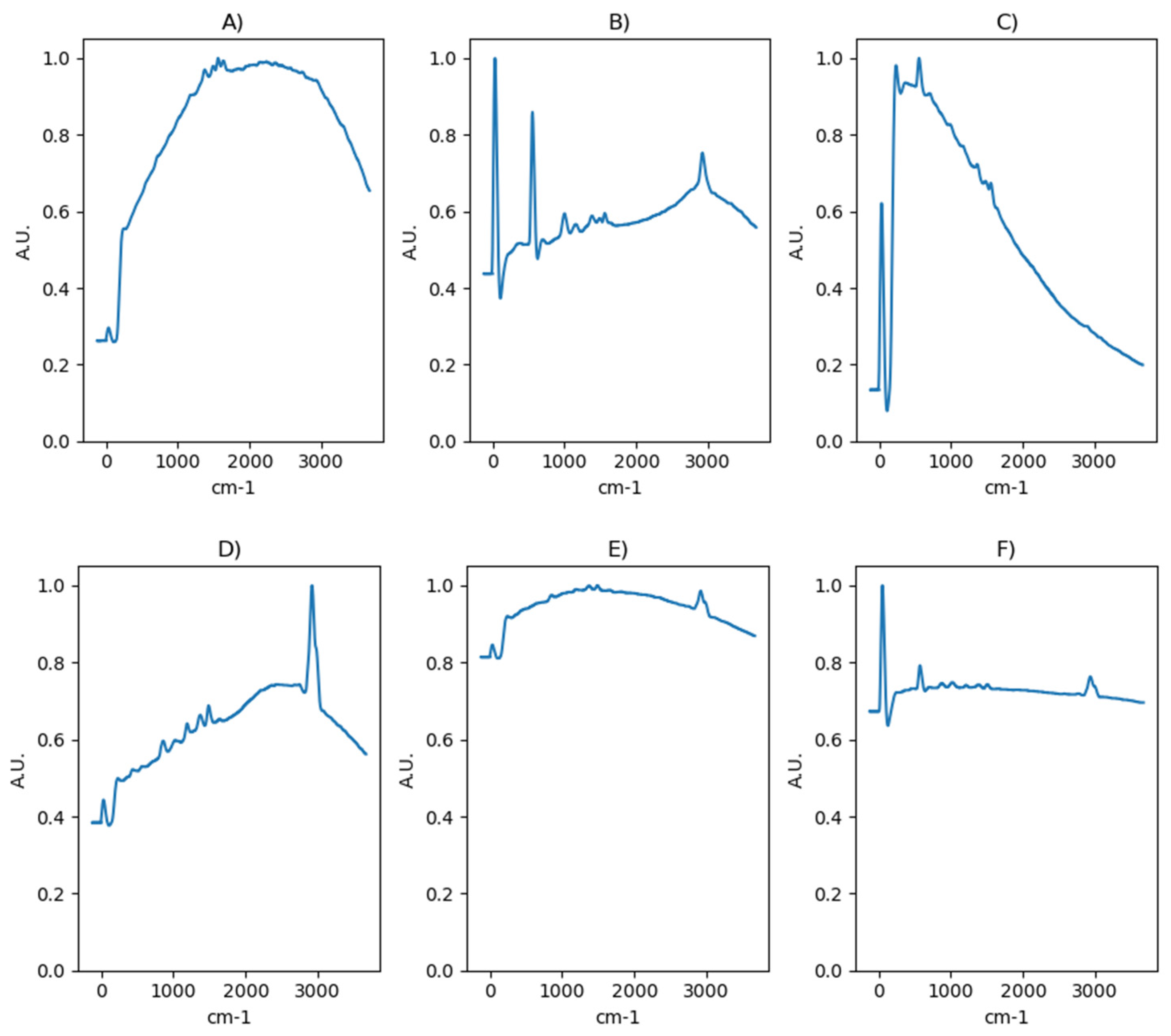
Only natural environmental samples were included, ensuring that the dataset reflects real-world conditions of microplastic contamination. As illustrated in Figure 1, panels A–C show Raman spectra corresponding to epoxy resin (ER) samples, while panels D–F represent polypropylene (PP) samples. The differences in baseline levels and overall noise intensity between spectra belonging to the same type of polymer are very noticeable. This intraclass variability can be attributed to the fluorescence background, the sample morphology, and even instrumental noise. They jointly affect the baseline and the relative intensities of the peaks. In addition, baseline variations and noise amplitude indicate a heterogeneous signal quality within each class. These variations reflect sample-dependent noise sources inherent to in situ marine sampling conditions.
All computational analyses were implemented in the Python (v3.10) programming environment. The development and execution of data preprocessing and machine learning models were performed using the libraries listed in Table 2, which provide robust and widely adopted frameworks for numerical computation, data handling, and deep learning tasks.
The computational procedures were carried out on a Dell Precision T3600 workstation equipped with an Intel® Xeon® processor, 32 GB of RAM, an NVIDIA GPU containing 1408 CUDA cores, and a 1 TB solid-state drive (SSD), ensuring efficient data processing and model training performance.

2.2. Preprocessing

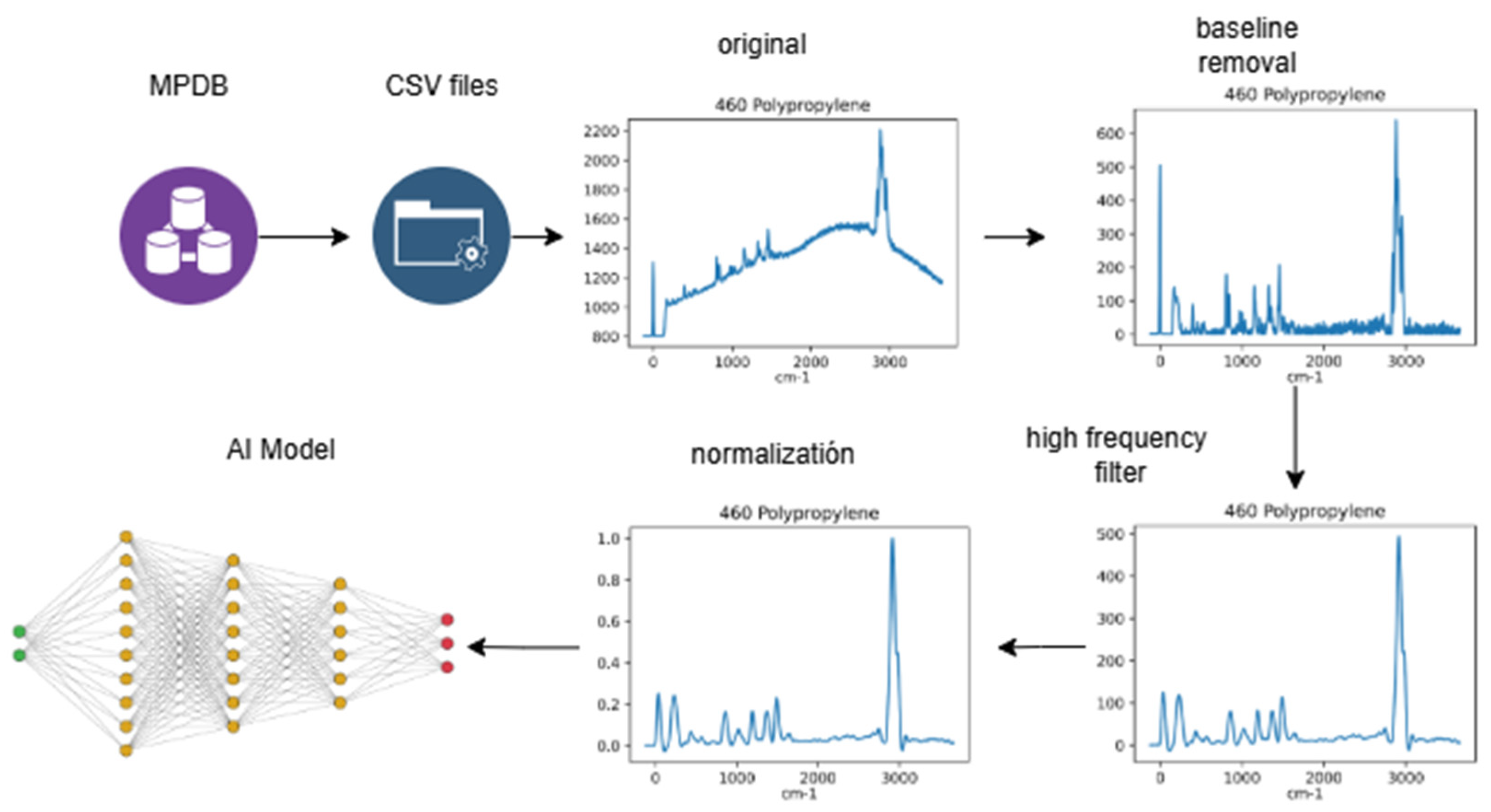
Two methodologies were used, conventional henceforth called as typical and peak-based representation henceforth called as canonical spectral transformation (CST). Typical preprocessing involves three fundamental stages: 1. Baseline removal, 2. High-frequency noise reduction, all spectra were smoothed using a third-order Butterworth low-pass filter with a normalized cutoff frequency of 0.05, effectively suppressing high-frequency noise, and 3. Normalization, as illustrated in Figure 2.
In addition to including high-frequency noise reduction and normalization procedures, CST focuses on the extraction of main features. It emphasizes the explicit representation of the coefficients of the Fourier series, which can be visualized with vertical bars for discrete data such as frequency—magnitude and phase—values. This can be considered a form of spectra, allowing standardization and simplification for more efficient analysis while preserving the integrity of spectral features. Additionally, the data were normalized in the CST using the Standard Scaler algorithm (z-score normalization) from Scikit-Learn’s Preprocessing module. Each spectra was adjusted to a mean value close to zero and a standard deviation of one. To preserve the integrity of subtle spectral features, standardized values were maintained with a precision of six decimals. This level of detail was chosen to ensure that minor but relevant Raman shifts and intensity variations were available for the AI models, avoiding the potential loss of information associated with lower-precision rounding.
All preprocessing steps associated with the Canonical Spectral Transformation were executed independently within each fold of the 10-fold cross-validation scheme, using exclusively the training data of each fold.
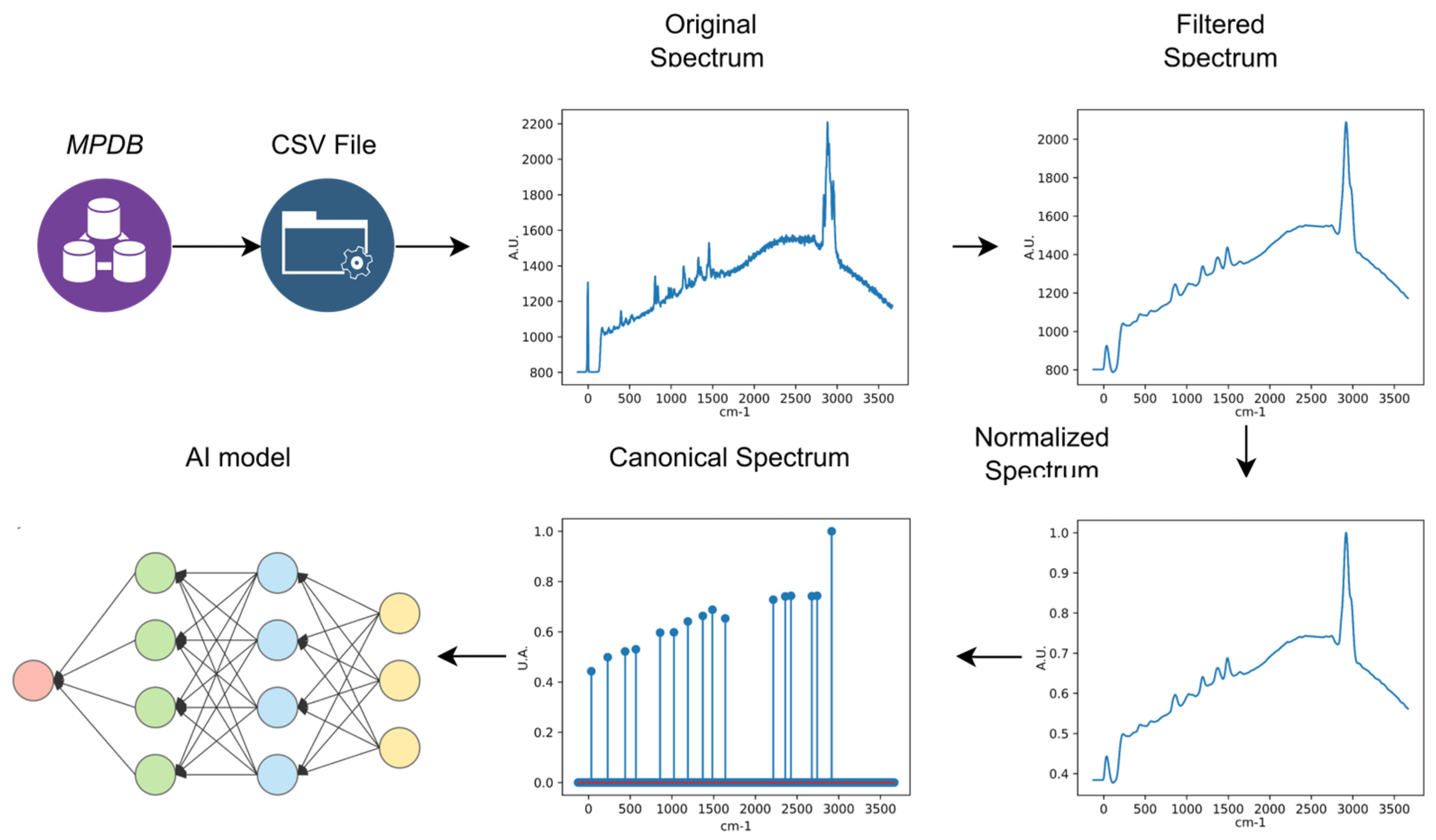
The proposed CST, illustrated in Figure 3, in addition to including the stages of typical preprocessing—high-frequency noise reduction and normalization procedures—incorporates a transformation stage that converts the spectra into a standardized canonical form, producing the canonical spectra. This latter is the source that feeds the AI model to be evaluated.

2.2.1. CST Algorithmic Implementation

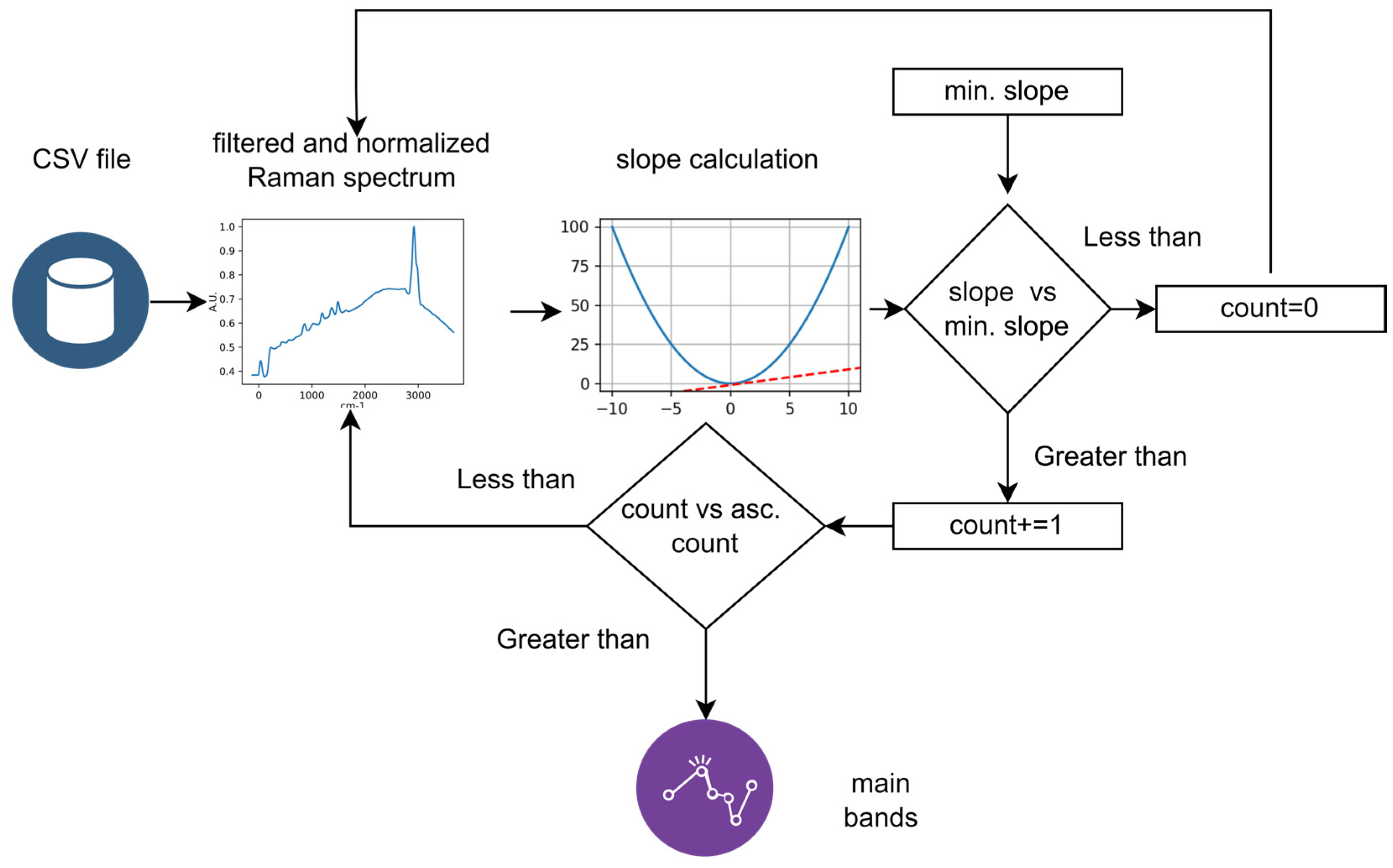
The core section of the CST is the detection of the characteristic vibrational bands of MPs. The principal band detection algorithm was developed based on a derivative-based slope analysis, the Slope calculation is based on Equation (1) where mi represents slope at point i, A represents the Raman intensity and v the Raman shift (cm−1). To distinguish genuine vibrational bands from stochastic noise, two critical hyperparameters were also used: slope (Slope threshold) and count (Persistence threshold). As illustrated in Figure 4, the algorithm evaluates the slope between consecutive spectral points and compares it with the predefined threshold. Consecutive points with slopes exceeding this value are accumulated until the ascending count criterion is satisfied, indicating a potential local maximum corresponding to a principal band. When the slope direction changes, the current coordinate is stored as the peak position, and the counter is reset. If the ascending sequence does not reach the required count, the algorithm continues scanning subsequent data points.
m i = A i + 1 A i ν i + 1 υ i

2.2.2. Creation of the Canonical Spectra Transformation

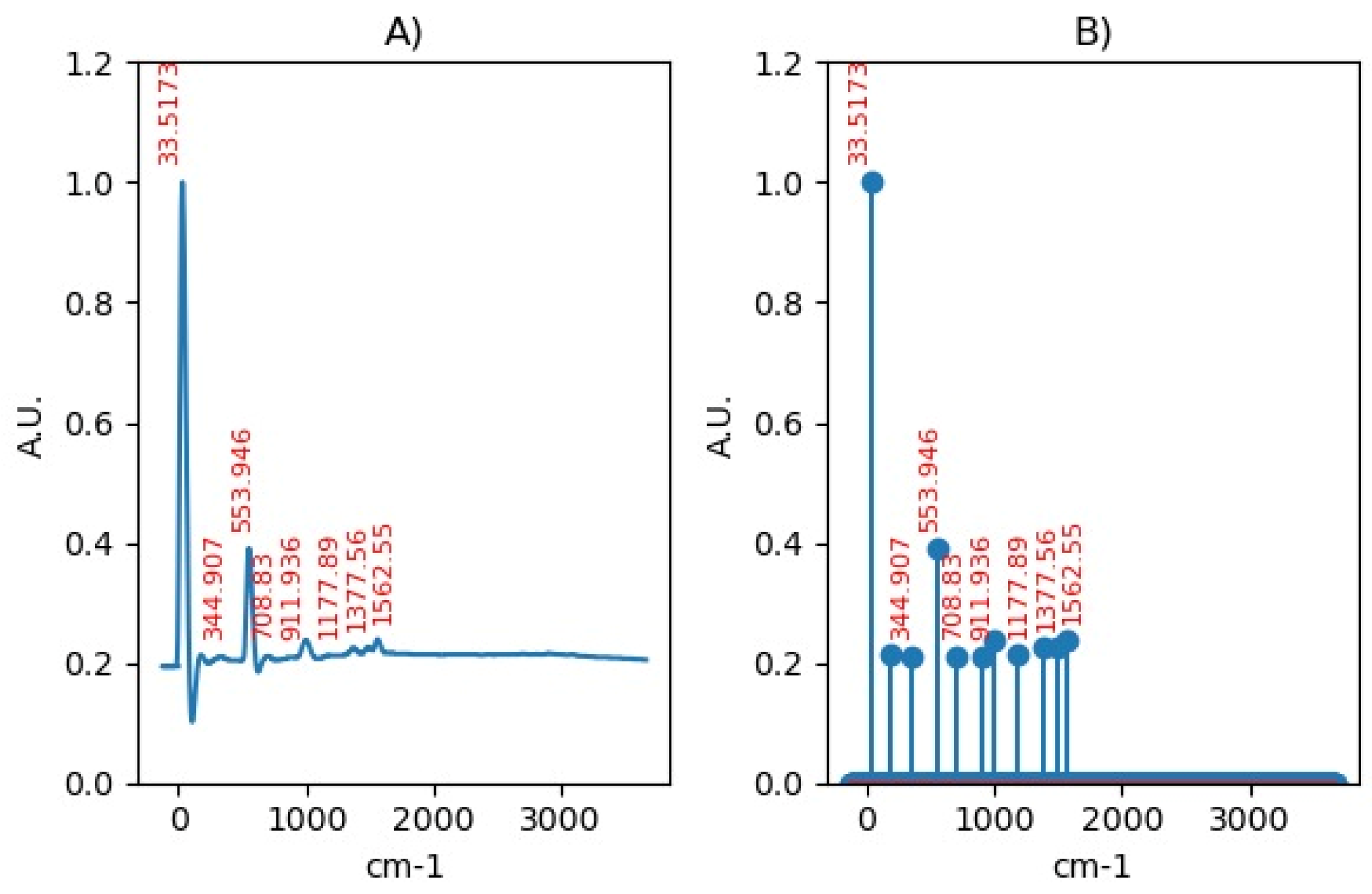
After the identification of the principal Raman bands, a Canonical Spectra (CST) was constructed. The original 1600-point spectra was replaced by a 1600-point vector, in which only the coordinates of the detected bands are retained with their corresponding magnitudes, all the remaining values are null. This representation reduced the data to approximately 10–20 non-zero entries, enabling efficient learning while maintaining essential spectral features. The full set of canonical spectra was subsequently provided to the AI models for classification. An illustrative example of this transformation is shown in Figure 5.

2.3. AI Models Used in Identification

Five AI models were employed to classify the Raman spectra of microplastic samples. Classical machine learning algorithms—including KNN, RF and MLP—were selected because they can achieve high classification accuracy even with relatively small datasets. In addition, the XGBoost algorithm was incorporated, which integrates ensembles of decision trees optimized through stochastic gradient descent using second-order Taylor and Newton–Raphson approximations. Finally, a CNN-1D was implemented as a deep learning approach capable of automatically extracting the most representative spectral features without manual preprocessing.

2.3.1. k-Nearest Neighbor

The KNN classifier relies on two principal tuning parameters: the number of nearest neighbors (k) and the metric defining inter-sample distance. Model generalization is highly sensitive to these parameters. A small k tends to increase variance and fit to noise, while a large k oversimplifies class boundaries. Although the Euclidean metric is standard, alternative measures—such as Manhattan or Minkowski—can improve performance when feature spaces are high-dimensional or exhibit unequal scaling across variables [28]. The configuration space evaluated for KNN optimization is summarized in Table 3.
The KNN model determines the class of a new instance by analyzing the k closest samples in feature space and assigning the label most prevalent among them. The influence of the neighborhood is estimated through the weight parameter, which can assign either equal relevance or distance-dependent relevance. The Minkowski distance is determined by p, resulting in the Manhattan metric for p = 1 and the Euclidean metric for p = 2. The metric parameter defines the distance used to measure similarity between samples and, therefore, determines the neighborhood configuration. In this case, the overall performance of the model was quantified using a relative performance index, which integrates classical evaluation measures such as accuracy, precision, and recall.

2.3.2. Random Forest

In the RF algorithm, to control the complexity of the model and the maximum depth allowed for each decision tree, the max_depth parameter is used. This way, it is possible to control how complex the model will be and the degree of interaction. The n_estimators number specifies the total number of decision trees generated and added to form the forest. The hyperparameter responsible for determining the number of features randomly considered to find the optimal split at each node is max_features, introducing stochasticity and promoting model generalization. On the other hand, the min_samples_leaf parameter defines the minimum number of samples required to form a leaf node, which represents a terminal node, so no further splits will be generated. The configuration for RF optimization is summarized in Table 4.

2.3.3. Multilayer Perceptron

In the MLP model, the hidden_layer_sizes parameter defines the network architecture, with each element of the tuple representing the number of neurons in the corresponding hidden layer. The length of the tuple defines the total number of hidden layers. The activation parameter specifies the nonlinear transformation applied to the weighted sum of inputs at each neuron, enabling the network to learn complex, non-linear relationships. Common activation functions include Sigmoid, Tanh, and Rectified Linear Unit (ReLU), each introducing distinct nonlinearity characteristics into the model.
The solver parameter defines the optimization algorithm used to update the network’s weights and biases by minimizing the loss function. It is important to prevent overfitting by penalizing large weights, which is achieved using the alpha parameter that represents the strength of the L2 regularization term, indicating weight decay. The learning rate hyperparameter controls the value of weight updates during training and affects both the speed of convergence and the stability of the optimization process. The configuration evaluated for MLP optimization is shown in Table 5.

2.3.4. Extreme Gradient Boosting

In the XGBoost model, the booster parameter sets the type of base learner used in the process. For each tree, a fraction of randomly selected training observations must be set, and the subsample hyperparameter is responsible for performing this task. This fraction acts as a regularization mechanism that reduces overfitting and promotes model generalization. The Eta parameter, also called the learning rate, sets the contribution of each tree during boosting iterations to adjust the step size of the weight updates. The colsample_bytree parameter regulates the fraction of features (columns) randomly sampled for each tree in the ensemble, providing an additional layer of regularization and diversity among base learners. The configuration space evaluated for XGBoost optimization is summarized in Table 6.

2.3.5. Convolutional Neural Network

The CNN architecture was originally introduced by Yann LeCun, who formulated the backpropagation algorithm for supervised training in the early LeNet model [29]. The architecture was further refined and demonstrated superior classification performance on the MNIST handwritten digit dataset [29]. Typical CNN architecture consists of three main components: (i) A convolutional block responsible for feature extraction, (ii) an intermediate block composed of dropout, max-pooling, and flattening layers for dimensionality reduction and regularization, and (iii) a fully connected block for final classification. In the convolutional stage, a moving receptive field scans the input sequence and applies convolution operations followed by bias addition and non-linear activation. This process produces feature maps that retain spatial or sequential dependencies in the data. A key property of convolutional layers is translation invariance, meaning that small input shifts result in proportionally shifted outputs without altering the extracted features [30]. While two-dimensional (2D) convolutional layers are commonly used in image analysis, one-dimensional (1D) CNNs are better suited for sequential data such as time series, text, audio, or spectral signals, making them particularly appropriate for Raman spectroscopy applications. The configuration space evaluated for CNN optimization is summarized in Table 7.
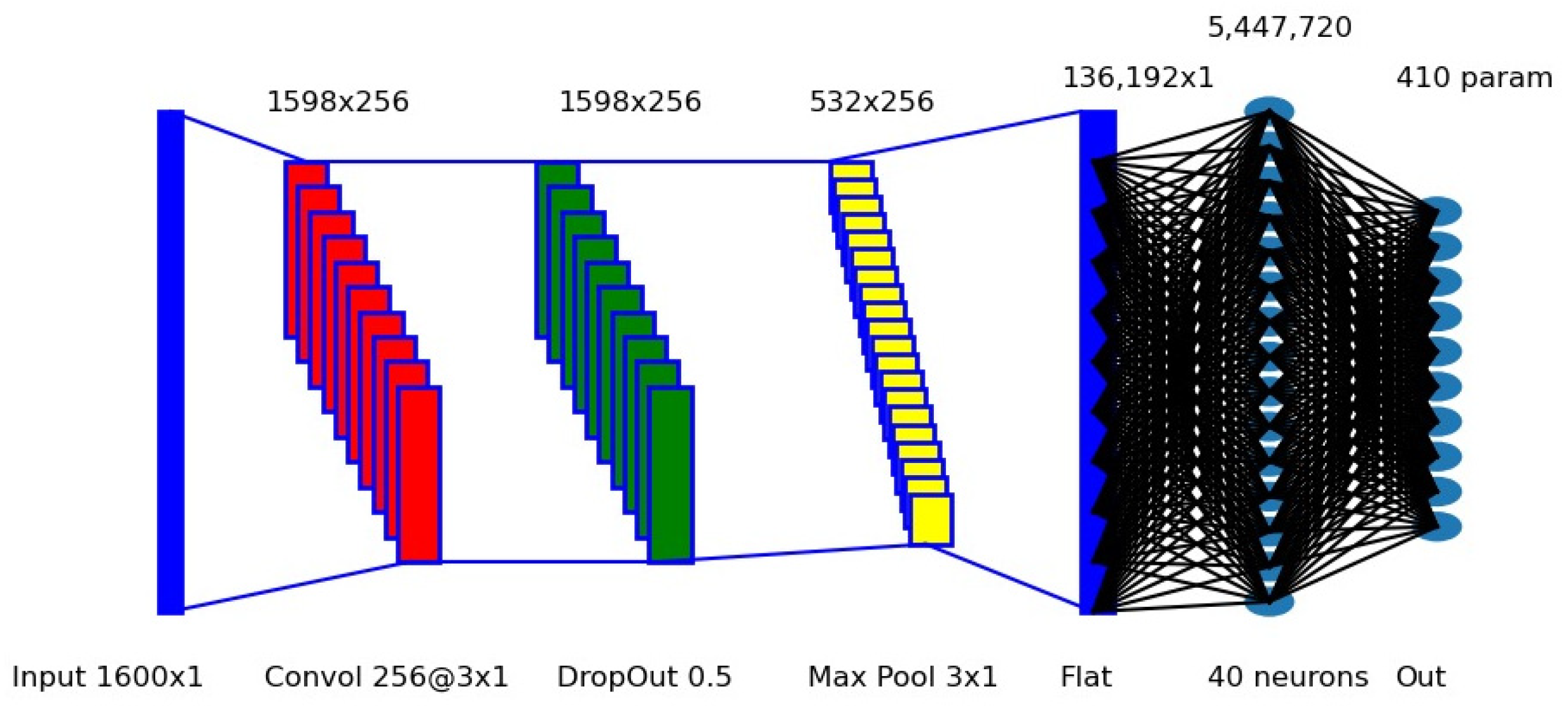
The CNN-1D architecture used in this study receives an input vector of 1600 points, corresponding to the intensity values of each Raman spectra. The model includes a convolutional layer with 256 filters of kernel size 3 × 1, followed by dropout and max-pooling layers (pool size = 3 × 1) for regularization and dimensionality reduction. The resulting feature maps are then flattened and passed to a fully connected dense layer comprising 40 neurons activated by the ReLU function. Finally, a softmax output layer produces the probability distribution across polymer classes, as illustrated in Figure 6.

3. Results

The classification performance of the five artificial intelligence models—RF, KNN, MLP, XGBoost and CNN—was evaluated using two distinct preprocessing strategies: the typical and the CST described in Figure 2 and Figure 3 (Section 2.1).
Each model was independently trained and validated on the balanced dataset of ten representative microplastic types (Table 1). All models were evaluated using stratified 10-fold cross-validation, where in each fold 90% of the data were used for training and 10% for testing. Performance metrics were averaged across folds to ensure robust evaluation.
Model stability and potential overfitting were assessed through cross-validation consistency rather than learning curves. Accuracy, precision, F1-score, and recall were computed for each fold, and their averaged values were used to evaluate robustness and unbiased evaluation across all preprocessing strategies. The close agreement between these metrics across folds indicates stable learning behavior and limited overfitting.

3.1. k-Nearest Neighbor

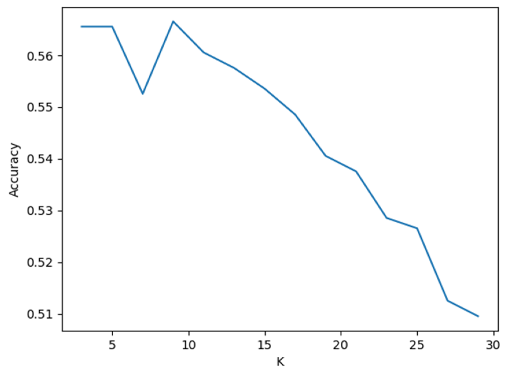
The optimization of the k parameter in the KNN model was first examined using typically preprocessed Raman spectra. The resulting accuracy curve (Figure 7) revealed that the best classification performance was achieved for k = 5 and k = 10, both providing stable convergence and consistent accuracy across validation folds.
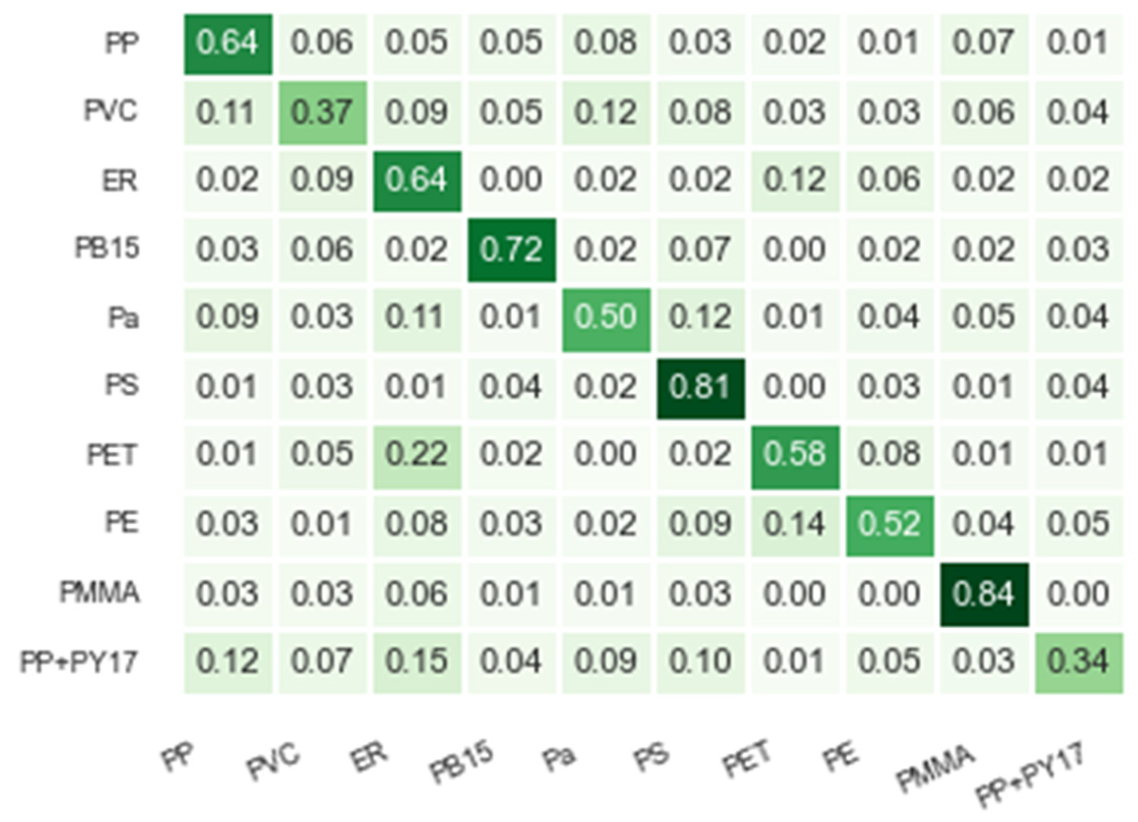
The confusion matrix of the KNN model with standard preprocessing (Figure 8) shows a clear diagonal predominance, although significant classification errors are observed in specific classes. Notably, PVC, PP+PY17, and Pa showed the lowest prediction rates. This decrease in performance for PVC and PP+PY17 can be attributed primarily to the similarity between their aliphatic chains. Conversely, PS and PMMA obtained the highest identification scores, likely due to their distinct and well-defined aromatic Raman bands.
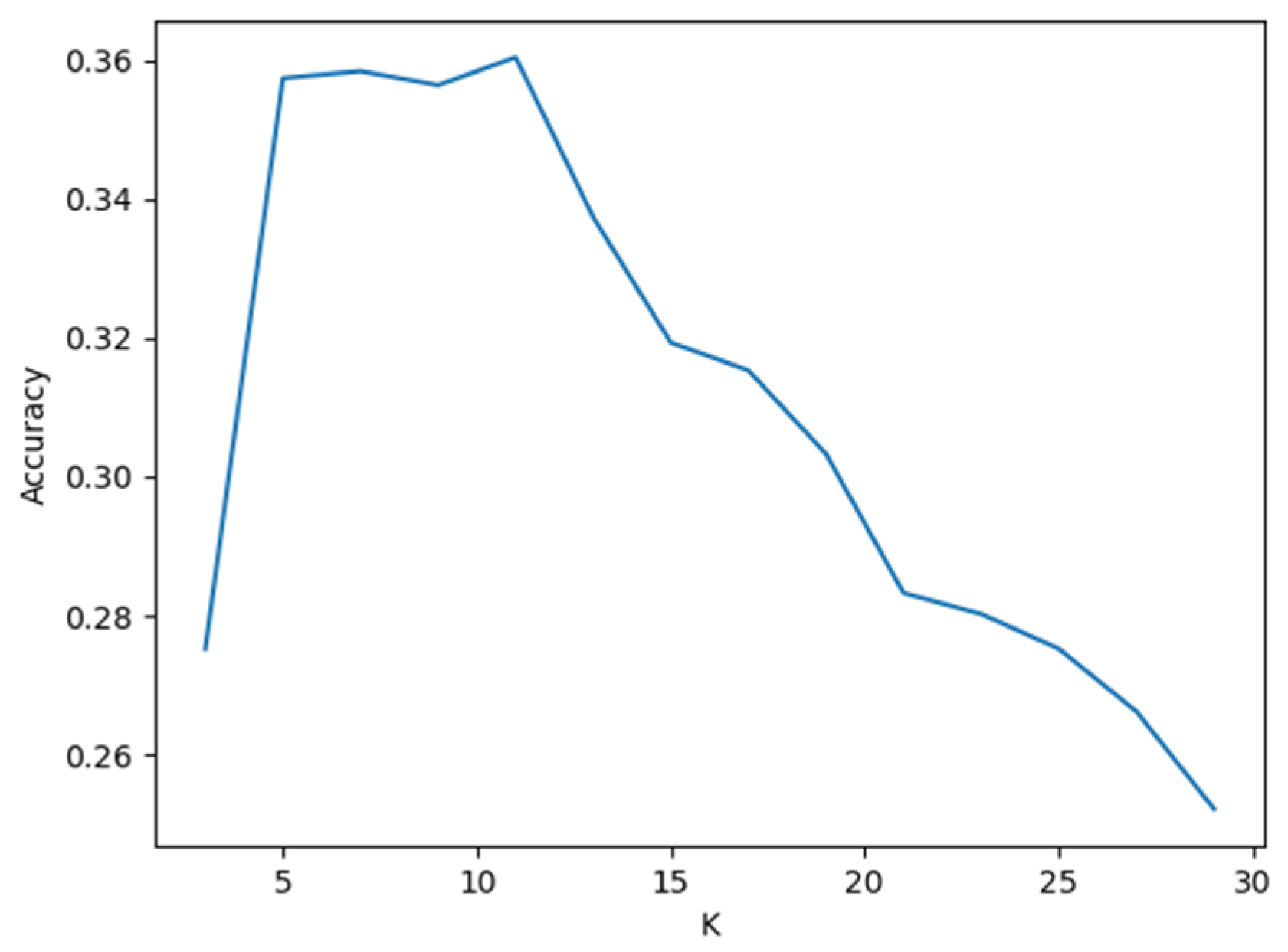
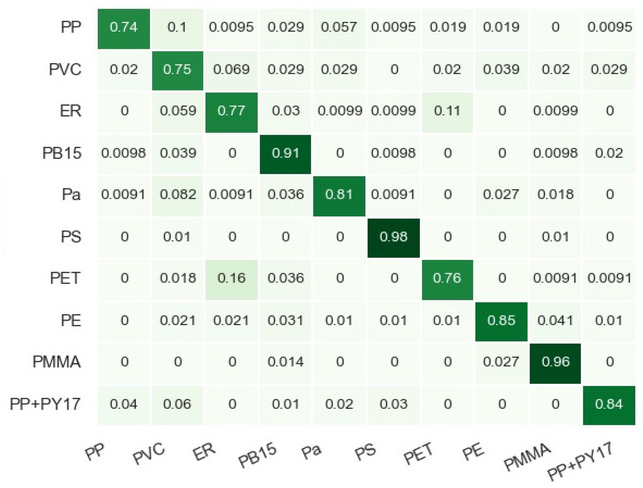
When CST was applied, the model demonstrated superior interclass separation. As shown in the neighbor parameter optimization (Figure 9, k = 5 and k = 12), CST effectively reduces intraclass variance while maximizing the distance between different polymer centroids. This is reflected in the confusion matrix (Figure 10), where classes such as PMMA and PS achieved near-optimal recognition. This improvement suggests that CST acts as a crucial step in the prediction of polymers.

3.2. Random Forest

The RF model under typical preprocessing (Figure 11) demonstrates its inherent ability to handle spectral nonlinearity thanks to its ensemble architecture. Greater classification success was observed for polymers with distinctive spectral signatures, such as PS and PB15, where the decision trees effectively split the feature space by focusing on the dominant Raman peaks.
In contrast, the integration of CST (Figure 12) further optimized the model’s discriminative capacity, specifically for classes that initially exhibited lower intensity or greater spectral overlap. By highlighting the feature set using CST, the RF model achieved greater accuracy in identifying Ps and PB15. Thus, while RF is robust, CST facilitates the identification of more stable split points for the decision trees, effectively reducing the misclassification of low-intensity signals and improving the model’s generalizability.

3.3. Extreme Gradient Boosting

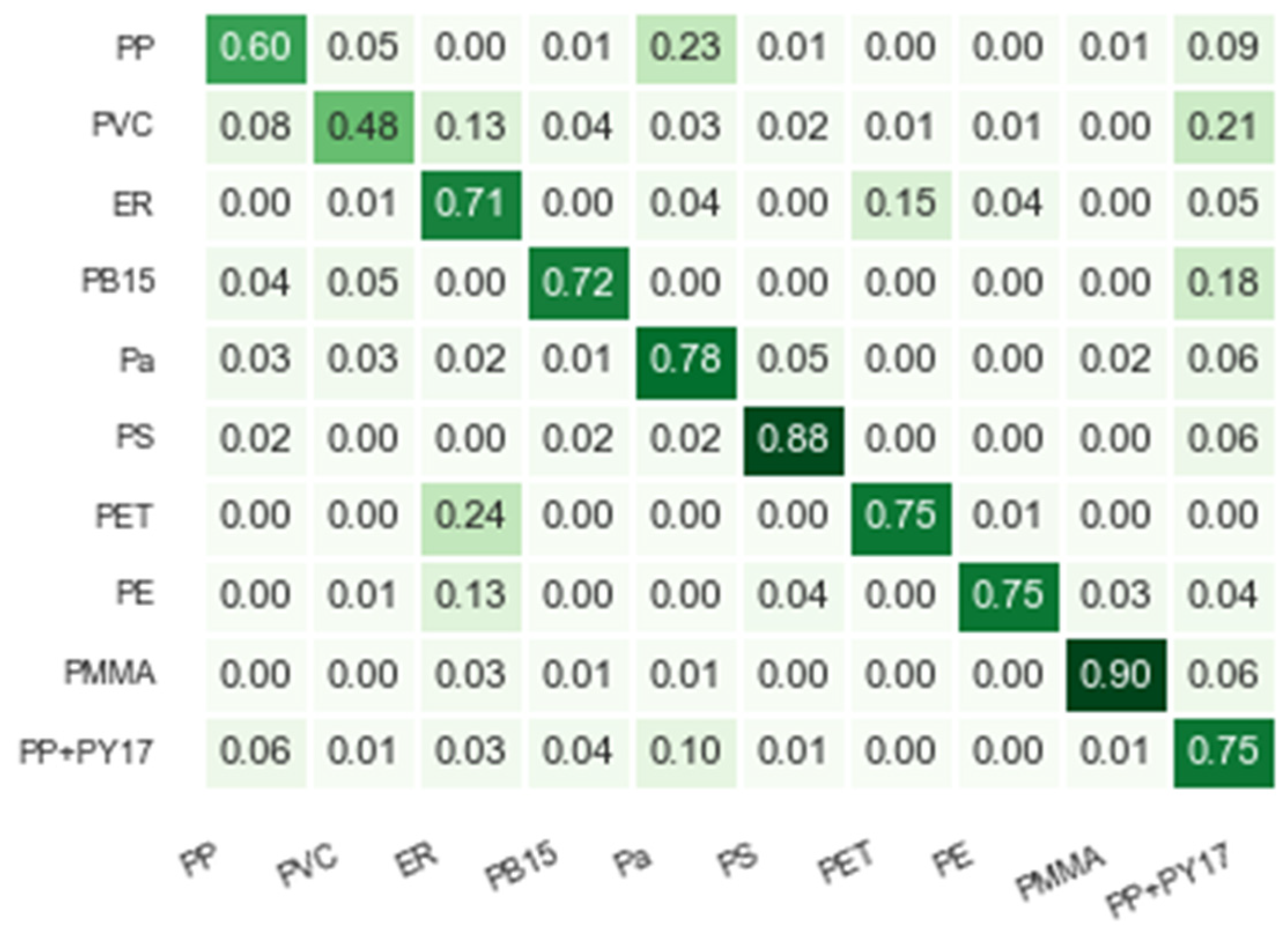
The performance of the XGBoost classifier, known for its efficiency in handling tabular data and nonlinear relationships, was initially evaluated using typical preprocessing (Figure 13). The model demonstrated robust feature selection capabilities, particularly for PS, where it effectively leveraged high-intensity vibrational modes. However, the misclassifications observed for PVC and ER suggest that, despite XGBoost’s regularized enhancement, spectral overlap and baseline similarities between these polymers still pose a significant challenge in handling unprocessed features.
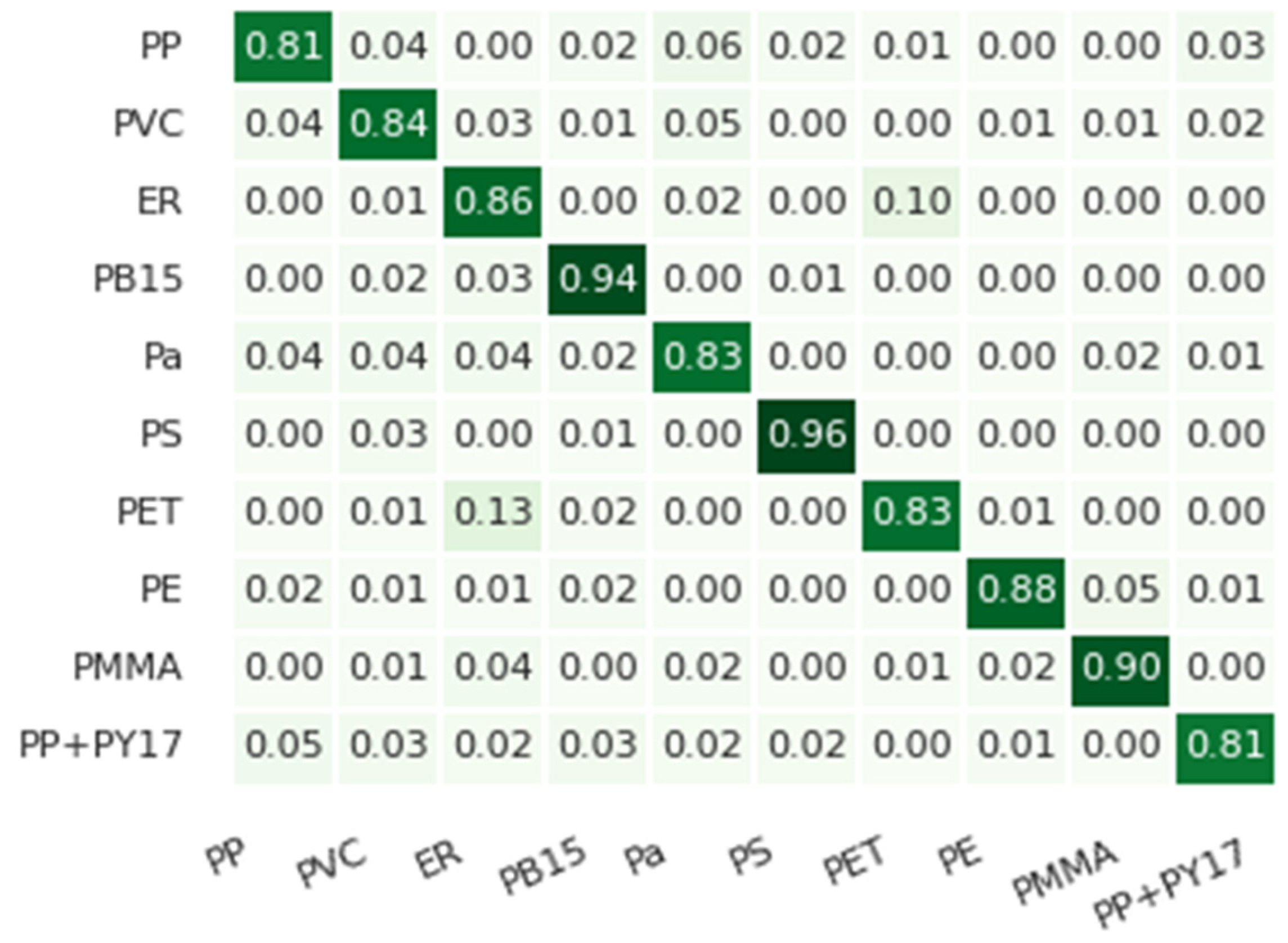
Implementing the CST approach (Figure 14) resulted in improved class separability. The model benefited from enhanced signal-to-noise ratios and the preservation of critical representative peaks. This is evident in the identification of PS, where CST reduced confounding with other acrylic polymers. The results indicate that CST acts as an important feature engineering step, allowing XGBoost to build more accurate decision trees by focusing on the most relevant spectral components and discarding redundant information.

3.4. Multilayer Perceptron

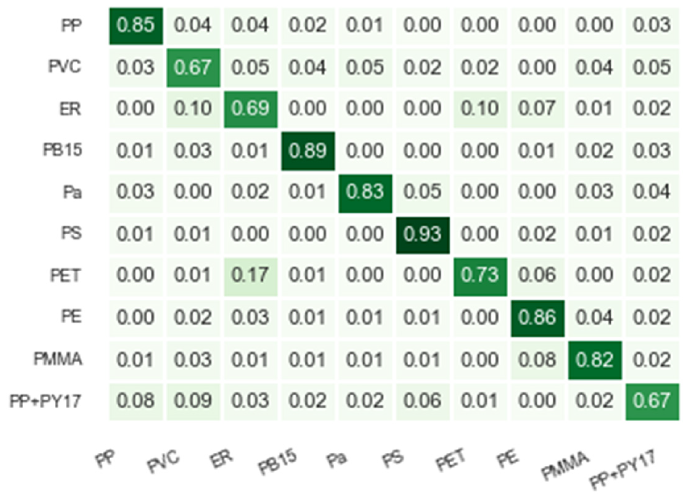
The MLP model was initially evaluated with standard preprocessing (Figure 15). While the model effectively identified the complex patterns of PMMA and PS, it exhibited significant difficulties with PVC and PP, where recovery rates fell below 60%. This performance gap highlights a common limitation of MLPs: the difficulty of converging on optimal weights when faced with high-dimensional Raman data that lacks clear linear separability or contains overlapping spectral data.
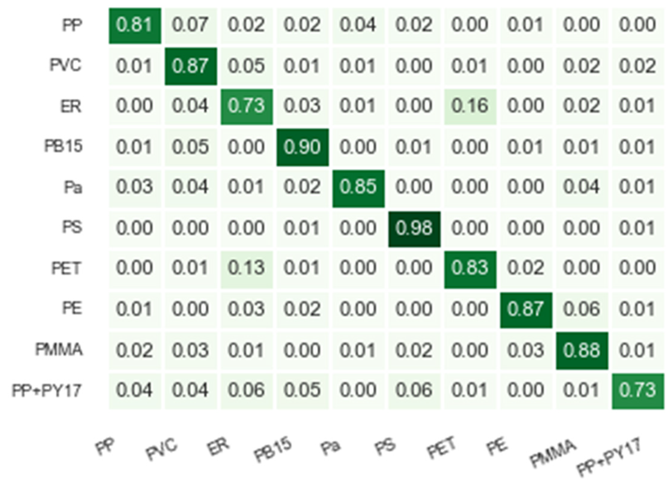
In contrast, the application of CST (Figure 16) promotes relevant optimization in the network learning process. By transforming the input features into a canonical space, intraclass variance was minimized, allowing the MLP to establish more defined decision boundaries. This is evidenced by the remarkable increase in prediction for PP+PY17, PS, and PMMA, with a reduction in class confusion exceeding 10%. These results demonstrate that CST acts as an essential conditioning step, facilitating superior generalization for neural network-based classifiers in microplastic identification.

3.5. Convolutional Neural Network

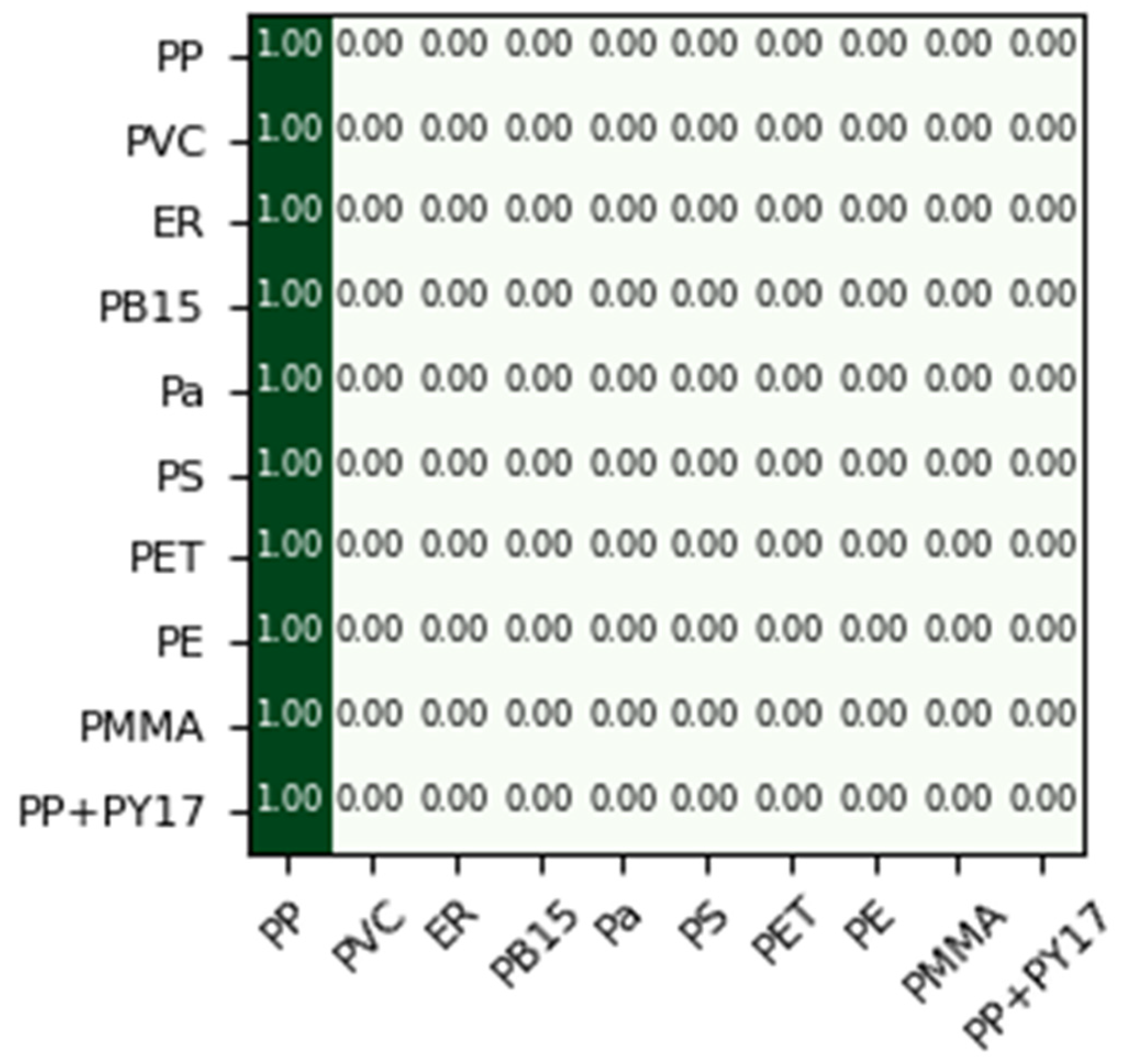
Using canonical preprocessing, the performance of the 1D-CNN model (Figure 17) showed a critical failure in achieving convergence, resulting in a classification accuracy close to random chance. This result suggests that the high-amplitude fluorescence and baseline instabilities inherent in raw Raman spectra act as unstructured noise, preventing the convolutional kernels from identifying stable hierarchical features. Despite the depth of the model (256 filters), stochastic gradient descent was unable to progress due to the high-entropy loss scenario presented by the unconditioned signals.
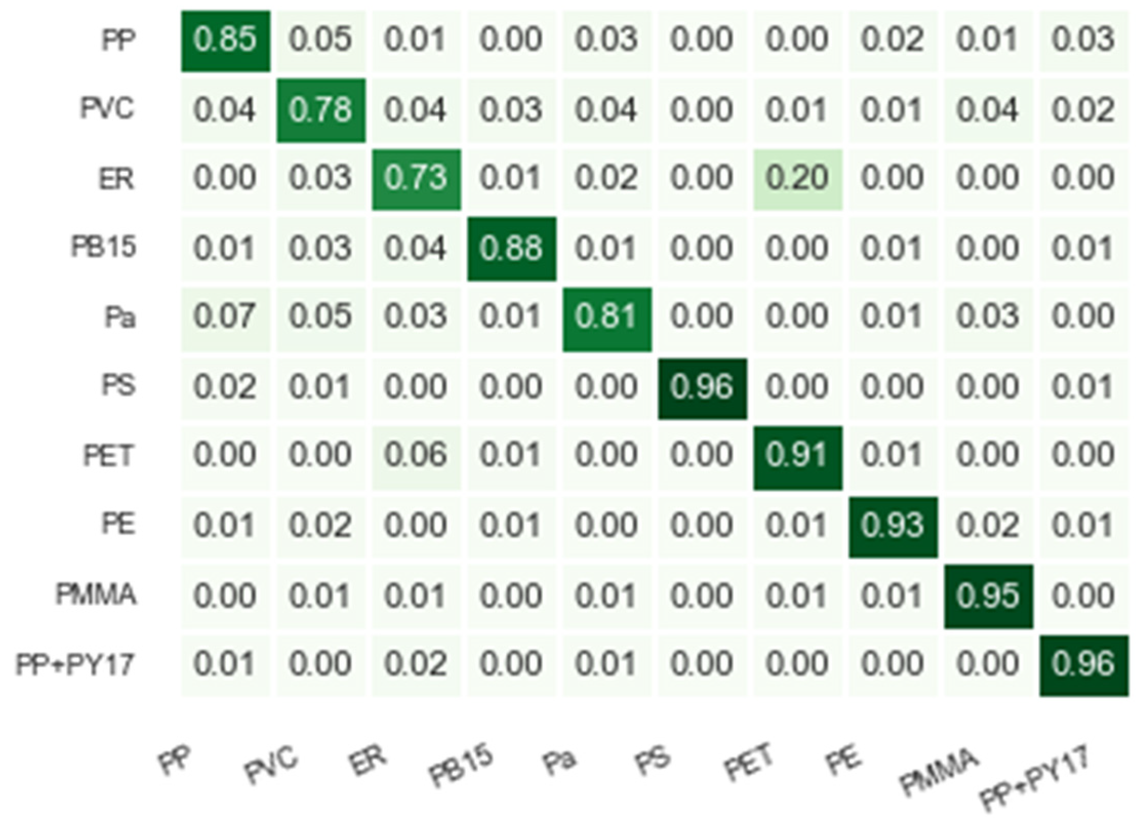
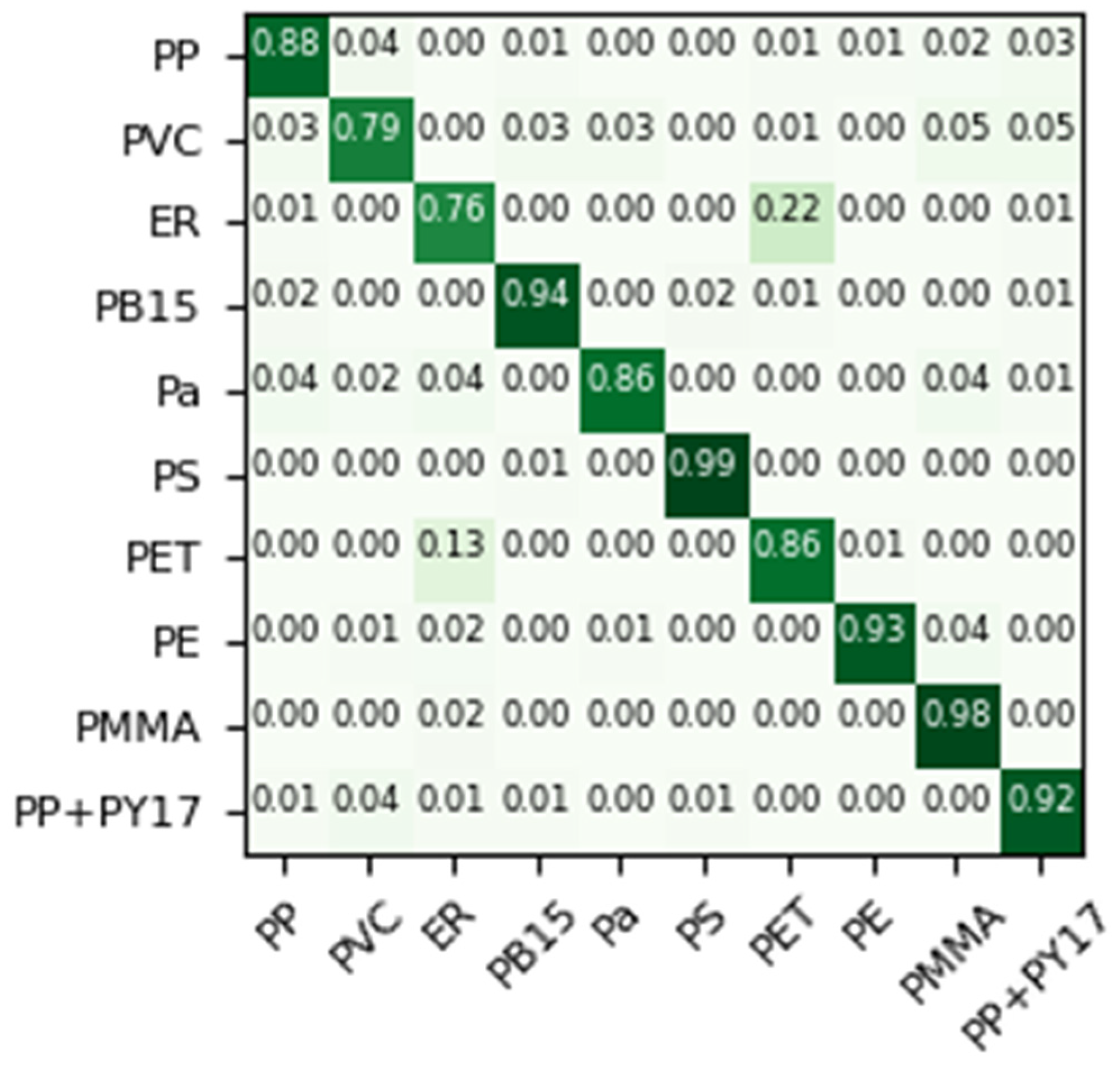
In contrast, the application of the CST approach (Figure 18) facilitated a rapid and robust convergence of the network. By standardizing the spectral topology, CST effectively highlighted the diagnostic vibrational bands, enabling the convolutional layers to extract highly discriminative patterns, indicating accurate classification for most categories and minimal overlap between classes. This is evidenced by the nearly perfect identification of PS and PMMA. The slight decrease in performance for ER is likely due to its broader spectral features, which are less distinctive compared to the sharp aromatic peaks of PS. Overall, the synergy between CNN and CST shows a clear diagonal dominance in the confusion matrix, which is essential for high-fidelity microplastic classification. In other words, CNN+CST allow signals that are difficult to process to be effectively transformed into a highly separable feature space.

3.6. Comparative Performance of AI Models

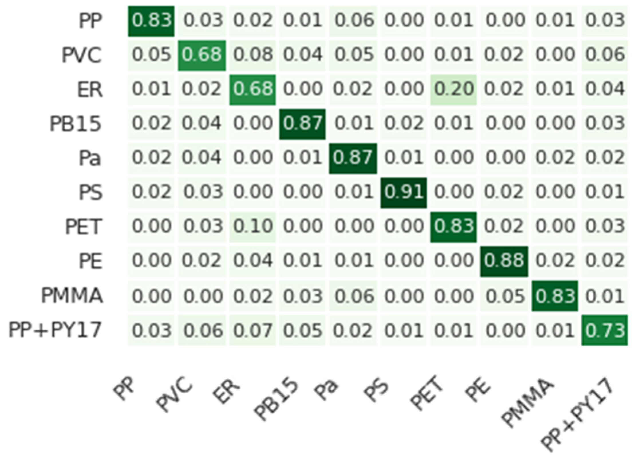
A comparative evaluation of the five AI models—KNN, RF, XGBoost, MLP, and CNN—was conducted, all of which were evaluated under typical preprocessing and CST. The main performance metrics were obtained: precision, recall, F1-score, and accuracy for both approaches. The results of this comparison are summarized in Table 8. It shows that all models, when using the CST, exhibit a consistent improvement.
Among the classical algorithms, CNN achieved the highest overall accuracy (0.90) under CST, outperforming MLP (0.88), XGBoost (0.84) and RF (0.83). It is important to notice that the CNN model had the best overall performance, obtaining 0.90 in all four metrics, thereby confirming its capacity to learn spectral patterns directly from CST normalized Raman data. In contrast, its performance on typically processed spectra remained negligible (accuracy = 0.10), underscoring the dependence of convolutional architectures on consistent and noise-reduced input representations.

3.7. Statistical Analysis

To evaluate the statistical significance of the performance improvements achieved by CST, a Wilcoxon test was conducted by Minitab Program v.22.1 (2024) ©. This non-parametric test was chosen to compare the paired performance of each model under Typical preprocessing versus CST for each model. An alternative hypothesis H1 was established: (ηCST − ηtyp) > 0, where ηCST represents the median accuracy of the CST approach and ηtyp corresponds to the median accuracy of the typical preprocessing. For a p-value below alpha = 0.05 (significance level) indicates that CST significantly outperforms typical preprocessing. As summarized in Table 9, all models yielded a p-value of 0.00296, well below the significance level of 0.05. This indicates that the null hypothesis is rejected, meaning that there is a significant difference between the medians of both sets. Furthermore, with H1 we conclude that the CST approach has a higher median than the typical median, clearly indicating that CST improves the prediction rate of each model.
To further evaluate which architecture provides the most robust classification under the CST approach, a pairwise comparison matrix was constructed (Table 10). The results indicate that the CNN model significantly outperforms all other evaluated architectures (KNN, MLP, XGBoost, and RF) with a consistent p-value of 0.003. This demonstrates that, while the CST approach improves each model, the hierarchical feature extraction capabilities of convolutional layers are particularly well-suited for the structured data produced by the canonical transformation. In contrast, comparisons between MLP, XGBoost, and RF showed p-values close to 0.998 in several cases, indicating that, although they are effective, there is no statistically significant difference in performance among these three when processing CST-Raman signals.

4. Discussion

The quantitative evaluation of the five artificial intelligence models revealed a strong dependence on the preprocessing strategy used. Although explicit feature importance metrics were not computed, the influence of key predictive factors can be inferred from the CST preprocessing framework. By transforming each spectra from approximately 1600 features to a limited set of dominant Raman bands, the models primarily relied on high-intensity vibrational modes associated with specific molecular bonds. This is a decisive factor in achieving successful MP classification.

4.1. Influence of Canonical Spectral Transformation

Considering that the samples with which the five artificial intelligence models were trained are natural, that is, taken directly from different seas [31], adding that organic contamination is evident and taking into account that the different Raman setups introduce inherent conditions, with all of the above, the true predictions of the five models evaluated under the CST improves from 20% to 100%. The performance increase between the typical and CST in the classification of the ten evaluated microplastics is evident. The CST method significantly enhanced the discriminative capability of the models by removing high-frequency noise and standardizing spectral baselines.
In Table 11, under the CST, the KNN model proved to be the best classifier for identifying PS with a score of true predictions of 0.98, while PVC went from true predictions of 0.37 to 0.75, improving its efficiency by 38%. In the case of the RF model, the results conclude that the best-classified microplastic was PS with a score of true predictions of 0.98, while PVC again showed an increase from 0.67 to 0.87, improving by 20%. For the XGBoost model, it showed true predictions of 0.96 for the classification of PS, the highest performance was for ER, which improved from 0.68 to 0.86, increasing its efficiency by 18%. Again, PS was best-classified using MLP with a score of true predictions of 0.97, while the highest true predictions performance was for PVC, going from 0.48 to 0.82, increasing its efficiency by 34%. Finally, CNN has definitively shown that the use of the typical approach was not able to classify any microplastic, while the CST demonstrated the best classification performance. That is, ER achieved an accuracy of 0.76 while PS achieved an accuracy of 0.99. In summary, it is evident that PS has been the best-classified microplastic in the five artificial intelligence models studied in this work, demonstrating the efficiency of the CST versus the typical approach.
The results indicate that CNN, MLP, and KNN models are capable of learning nonlinear relationships between the input variables and benefit more from the CST-based data representation, as it provides a physically meaningful encoding of vibrational peaks. On the other hand, instance-based algorithms, such as XGBoost, rely more on the spectral redundancy present in the raw Raman spectra and show less benefit from the transformed representation.

4.2. Spectral Overlap and Interference Analysis

The interference matrix Table 12 analysis as most misclassifications occurred between plastics sharing overlapping or closely spaced Raman bands. This indicates that prediction accuracy is strongly influenced by the presence, position, and intensity of characteristic vibrational modes rather than by secondary spectral information. The interference matrix was constructed summarizing the principal Raman bands of the polymers analyzed in this work [32,33]. The yellow cells indicate the most intense bands, while green cells denote secondary bands. The comparison between these bands and the false negatives from the confusion matrices revealed that classification errors predominantly occurred in polymers with overlapping vibrational modes, especially those sharing CH, C–C, or C–O–C bond contributions.
Spectral overlap between bands such as 1450–1460 cm−1 (CH2 bending) or 2900–2950 cm−1 (C–H stretching) was identified as the main cause of confusion between polymers such as PP–Pa, PVC–PP, and ER–PMMA. These overlaps correspond to bonds with similar vibrational energies, which generate near-identical Raman responses even when the polymeric backbone differs chemically.

4.3. Relationship Between Misclassification and Band Coincidence

The spectral interference analysis (Table 13) reveals that most false negatives arise in polymer pairs exhibiting Raman bands that are close or partially overlapping. Cases such as PP–Pa, PMMA–PE, and PP–PP+PY17 show clear vibrational proximity in the CH2 and aromatic stretching regions, which explains the model’s difficulty in separating these classes, even after CST. The highest false-negative values (e.g., PVC–PP and ER–PET) also correspond to polymers with strong band coincidences in the 800–1700 cm−1 and 2800–3000 cm−1 regions [33], indicating that the misclassifications originate from intrinsic chemical similarity rather than algorithmic limitations. Contradictorily, some pairs of polymers with overlapping characteristics, such as ER–PB15, do not generate false negatives, due to the use of CST, as long as the remaining spectral features or vibrational modes are sufficiently different to achieve correct classification. On the other hand, the low-frequency errors observed in pairs with minimal spectral overlap (for example, PB15–PS) suggest that the residual noise present in the MPDB dataset affects the classifier’s performance. In general, the analysis confirmed that most classification errors have a physical basis in the vibrational structure of the MPs, supporting the robustness of using CST and highlighting its ability to preserve chemically significant spectral information.
The above suggests that, although CST improves overall accuracy in all evaluated models, the intrinsic spectral overlap between chemically similar polymers remains a fundamental limitation for automatic classification based solely on Raman intensity data. Future work could mitigate this issue by integrating spectral fusion from multiple techniques (for example, combining Raman with FTIR or LIBS) or by incorporating different feature-level attention mechanisms to prioritize distinctive vibrational regions.

4.4. Effect of Noise and Sample Variability

Noise and baseline drift were identified as factors that limit the performance of the evaluated models. Although the CST substantially reduces the effects generated by high frequency and noise in the detection of low-frequency vibrational modes, specifically in PP, PE, and PMMA. This random interference explains small inconsistencies in the distributions of false positives (for example, PB15–PS and PET–ER), where the similarity in intensity causes more ambiguity than the frequency of the vibrational mode itself.
However, the overall results show that deep learning architectures combined with CST can achieve very high discrimination even under conditions of moderate noise, sample contamination, and equipment-induced noise, which validates CST as an effective tool for the identification of MPs from complex aquatic sources.
In summary, these results suggest that the most influential variables determining classification performance are the chemically significant Raman bands selected through canonical preprocessing, highlighting the physical interpretability of the proposed method as well as its higher accuracy. The proposed methodology outperforms traditional preprocessing in predictive accuracy and also provides a foundation for robust MP analysis using Raman spectra through AI models.
Although no fully independent external dataset was explicitly included, the MPDB represents a multi-laboratory and multi-instrument compilation of Raman spectra, implicitly incorporating cross-dataset and instrumental variability. This characteristic provides an initial level of robustness assessment for the proposed canonical spectral transformation within Raman spectroscopy. However, direct validation on external datasets and extension to other spectroscopic techniques remain important future research directions to further assess generalizability.
Several established feature extraction strategies have been applied to Raman spectroscopy data, including Principal Component Analysis (PCA), wavelet-based representations, autoencoder-derived embeddings, and vectors composed of intensities at predefined reference bands. These methods typically aim to transform or project spectral information into alternative representations that may optimize variance capture, multiscale decomposition, or compact encoding. In contrast, the proposed approach preserves the original spectral axis and dimensionality (1600 variables), generating a representation in which only the dominant vibrational bands are retained, while the remaining spectral positions are set to zero. This strategy emphasizes chemically significant Raman features without projecting the data into an abstract space.
Unlike PCA- and autoencoder-based methods, which generate transformed features that lack a direct physical correspondence to specific vibrational modes, CST maintains interpretability by explicitly associating nonzero values with characteristic Raman bands. Wavelet-based approaches and predefined peak intensity vectors, although effective under controlled conditions, often require prior expert knowledge and can be sensitive to peak shifts, fluorescence, and instrument variability, phenomena commonly observed in environmental Raman spectra, as is the case with the MPDB used in this research.
It is important to mention that this work offers an alternative that demonstrates that a sparse spectral representation, based on peaks of vibrational bands, can substantially improve classification performance in multiple machine learning models when applied to heterogeneous real-world marine samples. A systematic quantitative comparison with alternative feature extraction strategies will be addressed in future work.

5. Conclusions

The seawater samples used in this study were collected from the Baltic Sea and its surrounding areas, so the Raman spectra inherently contains noise, contamination, and instrumental variability. The purpose was to use natural samples so that they represented real conditions and could offer an efficient and accurate alternative for the identification of MPs.
A CST methodology was developed to extract the main features of Raman spectra for the identification of MPs in seawater samples. This method uses the original spectra and generates a new spectra using the CST. This preserves only the most important and representative vibrational features of the MPs while minimizing noise and redundancy. These results demonstrate that CST not only improves the extraction of spectral features from MPs for deep learning models but also provides an important foundation applicable to other spectroscopic modalities, such as Fourier Transform Infrared (FTIR) spectroscopy. This study demonstrates that, by extracting the frequency bands associated with molecular vibrational modes, the proposed method links data-driven approaches, offering a scalable pathway for the automated detection of MPs with high accuracy in aquatic environments. In other words, MPs can be identified in complex environments.
The identification of MPs using Raman spectroscopy can be significantly improved by combining AI models with CST preprocessing. While traditional models such as KNN, RF, and XGBoost offer reliable results, integrating CST with a 1D-CNN architecture represents a major breakthrough, achieving near-perfect classification accuracy.
Our results confirm a statistically significant performance leap (p = 0.00296$) across all evaluated models, with the 1D-CNN exhibiting the most dramatic evolution—transitioning from non-convergence to a near-perfect classification accuracy (median improvement of 0.867). The pairwise comparison matrix further underscores the superiority of the CST-CNN synergy, which provides a statistically distinct advantage (p = 0.003$) over traditional architectures. In conclusion, the integration of CST with deep learning models provides a robust, reproducible, and highly accurate methodology for the identification of MPs.

Author Contributions

Conceptualization, methodology, software, O.R.R.-V.; validation and formal analysis, M.C.M.-O.; investigation, O.R.R.-V. and M.C.M.-O.; resources, O.R.R.-V.; data curation, O.R.R.-V.; writing—original draft preparation, O.R.R.-V. and M.C.M.-O.; writing—review and editing, O.R.R.-V., M.C.M.-O., J.J.G.-S., A.M.-M., C.G.N.-D., R.N.-G., J.P.F.-D.l.R. and L.F.G.-O.; visualization, A.M.-M., C.G.N.-D., J.P.F.-D.l.R. and R.N.-G.; supervision, M.C.M.-O. and J.J.G.-S.; project administration, M.C.M.-O. and J.J.G.-S. All authors have read and agreed to the published version of the manuscript.

Funding

This work was also supported by the Consejo Nacional de Humanidades, Ciencias y Tecnologías (CONAHCyT) through the scholarship awarded to O.R Ruiz-Varela, whose contribution and dedication were fundamental to the completion of this study.

Data Availability Statement

The data used in this study were obtained from the Marine Plastic Database (MPDB), developed and maintained by the Leibniz Institute for Baltic Sea Research Warnemünde (IOW) as part of the BONUS Micropoll and MicroCatch projects. Access to the MPDB dataset was kindly provided by Dr. Cerkasova and her research team. The dataset is not publicly available due to data ownership and project restrictions but may be accessible upon reasonable request to the MPDB administrators at the IOW.

Acknowledgments

The authors express their sincere gratitude to Cerkasova and her research team for their support in granting access to the Marine Plastic Database (MPDB), which was essential for the development of this research.

Conflicts of Interest

The authors declare no conflicts of interest.

Abbreviations

The following abbreviations are used in this manuscript:
AIArtificial Intelligence
BONUSBaltic Organizations Network for Funding Science
CNNConvolutional Neural Network
CNN-1DOne-Dimensional Convolutional Neural Network
CSCanonical Spectra
EREpoxy Resin
ETLExtract, Transform, Load
FTIRFourier Transform Infrared Spectroscopy
GPUGraphics Processing Unit
IOWLeibniz Institute for Baltic Sea Research Warnemünde
KNNk-Nearest Neighbor
MLPMultilayer Perceptron
MPDBMarine Plastic Database
PaParafilm
PB15Phthalocyanine Blue 15
PEPolyethylene
PETPoly(ethylene terephthalate)
PMMAPoly(methyl methacrylate)
PPPolypropylene
PP+PY17Polypropylene with Pigment Yellow 17
PSPolystyrene
PTFEPolytetrafluoroethylene
PVCPoly(vinyl chloride)
RFRandom Forest
SGDStochastic Gradient Descent
XGBoostExtreme Gradient Boosting
z-scoreStandard score normalization (mean 0, SD 1)
CONAHCyTConsejo Nacional de Humanidades, Ciencias y Tecnologías (Mexico)
TPTrue Positive
TNTrue Negative
FPFalse Positive
FNFalse Negative

References

  1. ISO/TR 21960:2020; Plastics—Environmental Aspects—State of Knowledge and Methodologies. International Organization for Standardization: Geneva, Switzerland, 2020. Available online: https://standards.iteh.ai/catalog/standards/iso/fb95d3d6-569f-4fad-bf35-3718f99de839/iso-tr-21960-2020 (accessed on 27 March 2026).
  2. Andrady, A.L.; Neal, M.A. Applications and societal benefits of plastics. Philos. Trans. R. Soc. B Biol. Sci. 2009, 364, 1977–1984. [Google Scholar] [CrossRef]
  3. Geyer, R.; Jambeck, J.R.; Law, K.L. Production, Use, and Fate of All Plastics Ever Made. 2017. Available online: https://www.science.org/doi/10.1126/sciadv.1700782 (accessed on 27 March 2026).
  4. Hassan, I.; Sethupathi, S.; Bashir, M.J.K.; Munusamy, Y.; Chan, C.W. A systematic review of microplastics occurrence, characteristics, identification techniques and removal methods in ASEAN and its future prospects. J. Environ. Chem. Eng. 2024, 12, 112305. [Google Scholar] [CrossRef]
  5. Tsuchida, K.; Imoto, Y.; Saito, T.; Hara, J.; Kawabe, Y. A novel and simple method for measuring nano/microplastic concentrations in soil using UV-Vis spectroscopy with optimal wavelength selection. Ecotoxicol. Environ. Saf. 2024, 280, 116366. [Google Scholar] [CrossRef] [PubMed]
  6. Ragusa, A.; Notarstefano, V.; Svelato, A.; Belloni, A.; Gioacchini, G.; Blondeel, C.; Zucchelli, E.; De Luca, C.; D’avino, S.; Gulotta, A.; et al. Raman Microspectroscopy Detection and Characterisation of Microplastics in Human Breastmilk. Polymers 2022, 14, 2700. [Google Scholar] [CrossRef] [PubMed]
  7. Jones, J.I.; Vdovchenko, A.; Cooling, D.; Murphy, J.F.; Arnold, A.; Pretty, J.L.; Spencer, K.L.; Markus, A.A.; Vethaak, A.D.; Resmini, M. Systematic analysis of the relative abundance of polymers occurring as microplastics in freshwaters and estuaries. Int. J. Environ. Res. Public Health 2020, 17, 9304. [Google Scholar] [CrossRef] [PubMed]
  8. Kannan, K.; Vimalkumar, K. A Review of Human Exposure to Microplastics and Insights Into Microplastics as Obesogens. Front. Endocrinol. 2021, 12, 724989. [Google Scholar] [CrossRef]
  9. Jabeen, K.; Su, L.; Li, J.; Yang, D.; Tong, C.; Mu, J.; Shi, H. Microplastics and mesoplastics in fish. Environ. Pollut. 2017, 221, 141–149. [Google Scholar] [CrossRef]
  10. Lee, M.; Kim, H.; Ryu, H.-S.; Moon, J.; Khant, N.A.; Yu, C.; Yu, J.-H. Review on invasion of microplastic in our ecosystem and implications. Sci. Prog. 2022, 105, 368504221140766. [Google Scholar] [CrossRef]
  11. Chae, Y.; An, Y.J. Current research trends on plastic pollution and ecological impacts on the soil ecosystem: A review. Environ. Pollut. 2018, 240, 387–395. [Google Scholar] [CrossRef]
  12. Yang, X.; Man, Y.B.; Wong, M.H.; Owen, R.B.; Chow, K.L. Environmental health impacts of microplastics exposure on structural organization levels in the human body. Sci. Total Environ. 2022, 825, 154025. [Google Scholar] [CrossRef]
  13. Barceló, D.; Picó, Y.; Alfarhan, A.H. Microplastics: Detection in human samples, cell line studies, and health impacts. Environ. Toxicol. Pharmacol. 2023, 101, 104204. [Google Scholar] [CrossRef] [PubMed]
  14. Cressey, D. The plastic ocean. Nature 2016, 536, 263–265. [Google Scholar] [CrossRef]
  15. Rocha-Santos, T.; Duarte, A.C. A critical overview of the analytical approaches to the occurrence, the fate and the behavior of microplastics in the environment. TrAC Trends Anal. Chem. 2015, 65, 47–53. [Google Scholar] [CrossRef]
  16. Zhu, Y.; Li, Y.; Huang, J.; Zhang, Y.; Ho, Y.; Fang, J.K.; Lam, E.Y. Advanced Optical Imaging Technologies for Microplastics Identification: Progress and Challenges. Adv. Photonics Res. 2024, 5, 2400038. [Google Scholar] [CrossRef]
  17. Nava, V.; Frezzotti, M.L.; Leoni, B. Raman Spectroscopy for the Analysis of Microplastics in Aquatic Systems. Appl. Spectrosc. 2021, 75, 1341–1357. [Google Scholar] [CrossRef]
  18. Eberhardt, K.; Stiebing, C.; Matthaüs, C.; Schmitt, M.; Popp, J. Advantages and limitations of Raman spectroscopy for molecular diagnostics: An update. Expert Rev. Mol. Diagn. 2015, 15, 773–787. [Google Scholar] [CrossRef]
  19. Rossberg, N.; Gautam, R.; Komolibus, K.; O’Sullivan, B.; Visentin, A. Explainable AI-Based Feature Selection Approaches for Raman Spectroscopy. Diagnostics 2025, 15, 2063. [Google Scholar] [CrossRef]
  20. Fornasaro, S.; Alsamad, F.; Baia, M.; Batista de Carvalho, L.A.E.; Beleites, C.; Byrne, H.J.; Chiadò, A.; Chis, M.; Chisanga, M.; Daniel, A.; et al. Surface Enhanced Raman Spectroscopy for Quantitative Analysis: Results of a Large-Scale European Multi-Instrument Interlaboratory Study. Anal. Chem. 2020, 92, 4053–4064. [Google Scholar] [CrossRef]
  21. Lei, B.; Bissonnette, J.R.; Hogan, Ú.E.; Bec, A.E.; Feng, X.; Smith, R.D.L. Customizable Machine-Learning Models for Rapid Microplastic Identification Using Raman Microscopy. Anal. Chem. 2022, 94, 17011–17019. [Google Scholar] [CrossRef] [PubMed]
  22. Masaeli, M.; Fung, G.; Dy, J.G. From Transformation-Based Dimensionality Reduction to Feature Selection. In Proceedings of the 27th International Conference on Machine Learning, Haifa, Israel, 21–25 June 2010. [Google Scholar]
  23. Venkatesh, B.; Anuradha, J. A review of Feature Selection and its methods. Cybern. Inf. Technol. 2019, 19, 3–26. [Google Scholar] [CrossRef]
  24. Rytelewska, S.; Dąbrowska, A. The Raman Spectroscopy Approach to Different Freshwater Microplastics and Quantitative Characterization of Polyethylene Aged in the Environment. Microplastics 2022, 1, 263–281. [Google Scholar] [CrossRef]
  25. Jin, N.; Song, Y.; Ma, R.; Li, J.; Li, G.; Zhang, D. Characterization and identification of microplastics using Raman spectroscopy coupled with multivariate analysis. Anal. Chim. Acta 2022, 1197, 339519. [Google Scholar] [CrossRef]
  26. Zhang, W.; Feng, W.; Cai, Z.; Wang, H.; Yan, Q.; Wang, Q. A deep one-dimensional convolutional neural network for microplastics classification using Raman spectroscopy. Vib. Spectrosc. 2023, 124, 103487. [Google Scholar] [CrossRef]
  27. Čerkasova, N.; Enders, K.; Lenz, R.; Oberbeckmann, S.; Brandt, J.; Fischer, D.; Fischer, F.; Labrenz, M.; Schernewski, G. A Public Database for Microplastics in the Environment. Microplastics 2023, 2, 132–146. [Google Scholar] [CrossRef]
  28. Halder, R.K.; Uddin, M.N.; Uddin, M.A.; Aryal, S.; Khraisat, A. Enhancing K-nearest neighbor algorithm: A comprehensive review and performance analysis of modifications. J. Big Data 2024, 11, 113. [Google Scholar] [CrossRef]
  29. LeCun, Y.; Boser, B.; Denker, J.; Henderson, D.; Howard, R.; Hubbard, W.; Jackel, L. Handwritten digit recognition with a back-propagation network. In Proceedings of the 3rd International Conference on Neural Information Processing Systems, Denver, CO, USA, 27–30 November 1989. [Google Scholar]
  30. Xie, L.; Luo, S.; Liu, Y.; Ruan, X.; Gong, K.; Ge, Q.; Li, K.; Valev, V.K.; Liu, G.; Zhang, L. Automatic Identification of Individual Nanoplastics by Raman Spectroscopy Based on Machine Learning. Environ. Sci. Technol. 2023, 57, 18203–18214. [Google Scholar] [CrossRef] [PubMed]
  31. Böke, J.S.; Popp, J.; Krafft, C. Optical photothermal infrared spectroscopy with simultaneously acquired Raman spectroscopy for two-dimensional microplastic identification. Sci. Rep. 2022, 12, 18785. [Google Scholar] [CrossRef]
  32. Peñalver, R.; Zapata, F.; Arroyo-Manzanares, N.; López-García, I.; Viñas, P. Raman spectroscopic strategy for the discrimination of recycled polyethylene terephthalate in water bottles. J. Raman Spectrosc. 2023, 54, 107–112. [Google Scholar] [CrossRef]
  33. BONUS MICROPOLL: Multilevel Assessment of Microplastics and Associated Pollutants in the Baltic Sea. Available online: https://www.iow.de/project/192/micropoll.html (accessed on 17 July 2025).
Figure 1. Examples of Raman spectra of marine water samples contaminated with ER (AC) and PP (DF), belonging to the MPDB database.
Microplastics 05 00071 g001
Figure 2. The figure shows the steps involved in typical preprocessing. The files containing the original Raman spectra are extracted from the MPDB, then the baseline is removed, followed by the elimination of high-frequency noise, and finally normalization is performed before feeding the data into the AI model.
Microplastics 05 00071 g002
Figure 3. The figure shows the stages that make up the CST. The files containing the original Raman spectra are extracted from the MPDB, followed by the elimination of high-frequency noise, then the normalization stage is carried out, and finally the canonical spectra is generated before feeding the data into the AI model.
Microplastics 05 00071 g003
Figure 4. Outline of the derivative-based algorithm used for detecting principal Raman bands, illustrating the evaluation of local slopes, threshold comparison, and identification of peak coordinates. A peak is only recorded if the signal shows a sustained positive slope (slope > min slope) for a minimum number of points count. This ensures that high-frequency noise, which can produce high instantaneous slopes, lacks spatial persistence and is effectively filtered out without the need for smoothing that could distort the peak’s position.
Microplastics 05 00071 g004
Figure 5. Comparison of an original spectra (A) and a canonical spectra (B) for a sample of marine water contaminated with PB15, number 1441 in the MPDB Dataset.
Microplastics 05 00071 g005
Figure 6. Schematic representation of the CNN used for Raman-based microplastic classification, illustrating the convolution, dropout, pooling, flattening, and fully connected layers.
Microplastics 05 00071 g006
Figure 7. Estimation of optimal neighbor number (k) in the KNN model using typically preprocessed Raman spectra.
Microplastics 05 00071 g007
Figure 8. Confusion matrix for KNN classification using typical preprocessing.
Microplastics 05 00071 g008
Figure 9. Estimation of optimal neighbor number (k) in the KNN model using CST.
Microplastics 05 00071 g009
Figure 10. Confusion Matrix for KNN evaluating by CST using Raman spectra data.
Microplastics 05 00071 g010
Figure 11. Confusion matrix for Random Forest classification using typical preprocessing.
Microplastics 05 00071 g011
Figure 12. Confusion matrix for Random Forest classification by CST using Raman spectra data.
Microplastics 05 00071 g012
Figure 13. Confusion Matrix for XGBoost evaluating with typical sample preprocessing.
Microplastics 05 00071 g013
Figure 14. Confusion matrix for XGBoost classification by CST using Raman spectra data.
Microplastics 05 00071 g014
Figure 15. Confusion matrix for MLP by typical classification using Raman spectra data.
Microplastics 05 00071 g015
Figure 16. Confusion matrix for MLP classification by CST using Raman spectra data.
Microplastics 05 00071 g016
Figure 17. Confusion matrix for CNN by typical classification using Raman spectra data.
Microplastics 05 00071 g017
Figure 18. Confusion matrix for CNN by CST using Raman spectra data.
Microplastics 05 00071 g018
Table 1. Partial summary of polymer categories in the MPDB showing the number of Raman spectra available for each microplastic type.
Microplastic TypeAcronymNumber of Samples
Poly(ethylene terephthalate)PET21,769
Poly(tetrafluoroethylene)PTFE17,284
PolypropylenePP14,613
PolyethylenePE4972
PolystyrenePS4001
Poly(vinyl chloride)PVC3235
Phthalocyanine BluePB152120
ParafilmPa864
Poly(methyl methacrylate)PMMA808
Epoxy resin1ER655
Polypropylene + PY17basedPP+PY17561
Table 2. Python libraries were used for data processing and model development in this study.
LibraryApplication
keras v.2.12.0API deep learning
Pandas v.2.0.3Data management and csv
Matplotlib v.3.7.2Graphics generator
Numpy v.1.24.3Numerical computing
Sklearn v.1.3.0Data analysis
Tensorflow v.2.12.1Low level API Deep learning
Table 3. Summarizes the parameter space explored during KNN training for microplastic classification.
ParameterValues
neighbors (k)5, 7
weightsDistance
p1, 2
metricMinkowski, Mahalanobis, Seuclidean, Euclidean, Manhattan
Table 4. The ranges of hyperparameters evaluated during RF training for MPs identification using Raman spectral data are shown.
ParameterValues
max_depth3, 5, 7, 10
n_estimators100, 200, 300, 400, 500
max_features10, 20, 30, 40
min_samples_leaf1, 2, 4
Table 5. Parameter space used for training the MLP model for microplastic classification.
ParameterValues
hidden_layer_sizes(10,20,10), (15,20,20), (30,20,30)
activationTanh, ReLU
solverSGD, Adam
alpha0.0001, 0.05
learning rateconstant, adaptive
Table 6. Parameters used for training the XGBoost model for MPs classification.
ParameterValues
Boostergbtree, gblinear, dart
subsample0.2, 1.0
Eta0.1, 1.0
colsample bytree0.2, 1.0
Table 7. Parameter space used for training the CNN model for microplastic classification.
ParameterValues
Weight constraint1, 3, 5
Dropout rate0.1, 0.4, 0.9
Fully connected layers30, (30,30), 60
Table 8. Performance metrics obtained for the five AI models using typical and CST strategies.
ModelPre ProcessingPrecisionRecallF1-ScoreAccuracy
KNNTypical0.740.730.730.73
KNNCanonical0.830.830.830.83
RFTypical0.740.730.730.73
RFCanonical0.83 0.830.830.83
XGBoostTypical0.800.810.800.80
XGBoostCanonical0.850.850.850.84
MLPTypical0.780.770.770.77
MLPCanonical0.870.870.870.88
CNNTypical0.010.100.020.10
CNNCanonical0.900.900.900.90
Table 9. Statistical test by Wilcoxon using 10 folds and accuracy value.
ModelKNNMLPXGBoostRFCNN
p-value0.002960.002960.002960.002960.00296
Median Can-Typ > 00.0450.1740.04250.19750.86755
Table 10. Regarding the Wilcoxon statistical test to determine which classifier model performs best using CST approach, the same alternative hypothesis H1 is used again. The table shows the p-values for each comparison between models. It can be observed that the KNN classifier performed the worst, as the p-value for each comparison was less than the significance level of 0.05 (all p > 0.05). For the MLP classifier, its performance is better than the KNN (p = 0.003), XGBoost (p = 0.011), and Rf (p = 0.003) classifiers; however, it is not significantly better than the CNN classifier (p > 0.05). Regarding the CNN classifier, the p-value is less than the significance level of 0.05 in all cases, indicating that it is the model that performed best using the CST approach. Finally, we observed that the RF and XGBoost classifiers are mid-performance models that fall short of the performance of MLP and CNN.
ModelKNNMLPXGBoostRFCNN
KNN-0.9980.9980.9980.998
MLP0.003-0.0110.0030.998
XGBoost0.0030.992-0.0030.998
RF0.0030.9980.998-0.998
CNN0.0030.0030.0030.003-
Table 11. Summary of results. In blue, the greatest increase in the ranking of MPs according to the AI model is shown, while the best-ranked MP of each model is highlighted in bold.
MPKNNRFXGBoostMLPCNN
TypCanTypCanTypCanTypCanTypCan
PP0.640.740.850.810.830.810.600.911.000.88
PVC0.370.750.670.870.680.840.480.820.000.79
ER0.640.770.690.730.680.860.710.800.000.76
PB150.720.910.890.900.870.940.720.910.000.94
Pa0.500.810.830.850.870.830.780.870.000.86
PS0.810.980.930.980.910.960.880.970.000.99
PET0.580.760.730.830.830.830.750.880.000.86
PE0.840.850.860.870.880.880.750.960.000.93
PMMA0.340.960.820.880.830.900.900.950.000.98
PP+PY170.630.840.670.730.730.810.750.850.000.92
Maximum
True Prediction
38%20%18%34%99%
Table 12. Interference matrix of the analyzed polymers. Yellow cells represent the highest-intensity Raman bands; green cells indicate secondary intensities. Column headers specify the vibrational mode associated with each band.
MPC–CC–CCF3C–FC–O–CRING
Breath
CHC–CCH2CH2RING StretchRING StretchESTECH2CH2
PS 10011031 1602 29003050
PE 1062113012961417 2850
PET 630 856 1308 16151726
PP 832967 115013241454 28002950
PVC361636694 13301430 1590 29162940
PB15 680747 11421340 1529
ER 826 11161240 1585 29203071
Pa 814 1455 17302954
PMMA 829986 1451 172529452994
PP+PY 1443 1629 2916
Table 13. The interference matrix shows the Raman frequency bands associated with each pair of MPs analyzed [33]. The cells highlighted in yellow indicate the bands with the highest intensity, while the cells highlighted in green denote the bands with the second highest intensity. These bands reflect the vibrational modes that are most likely to contribute to spectral overlap and, consequently, to false negative classifications in the different models.
Plastic 1Plastic 2Freq (cm−1)Freq (cm−1)
PPPa814, 8321454, 1455
PB15PSxx
ERPET856, 826x
PMMAPE1417, 14512850, 2945
ERPMMA826, 8292945, 2920
PPPP+PY1443, 14542800, 2916
PVCPP1324, 13302950, 2940
PaPVC2916, 29541430, 1455
PETER826, 856585, 1615
ERPB151142, 11161240, 1340
Disclaimer/Publisher’s Note: The statements, opinions and data contained in all publications are solely those of the individual author(s) and contributor(s) and not of MDPI and/or the editor(s). MDPI and/or the editor(s) disclaim responsibility for any injury to people or property resulting from any ideas, methods, instructions or products referred to in the content.