Author Contributions
Conceptualization, methodology, software, O.R.R.-V.; validation and formal analysis, M.C.M.-O.; investigation, O.R.R.-V. and M.C.M.-O.; resources, O.R.R.-V.; data curation, O.R.R.-V.; writing—original draft preparation, O.R.R.-V. and M.C.M.-O.; writing—review and editing, O.R.R.-V., M.C.M.-O., J.J.G.-S., A.M.-M., C.G.N.-D., R.N.-G., J.P.F.-D.l.R. and L.F.G.-O.; visualization, A.M.-M., C.G.N.-D., J.P.F.-D.l.R. and R.N.-G.; supervision, M.C.M.-O. and J.J.G.-S.; project administration, M.C.M.-O. and J.J.G.-S. All authors have read and agreed to the published version of the manuscript.
Figure 1.
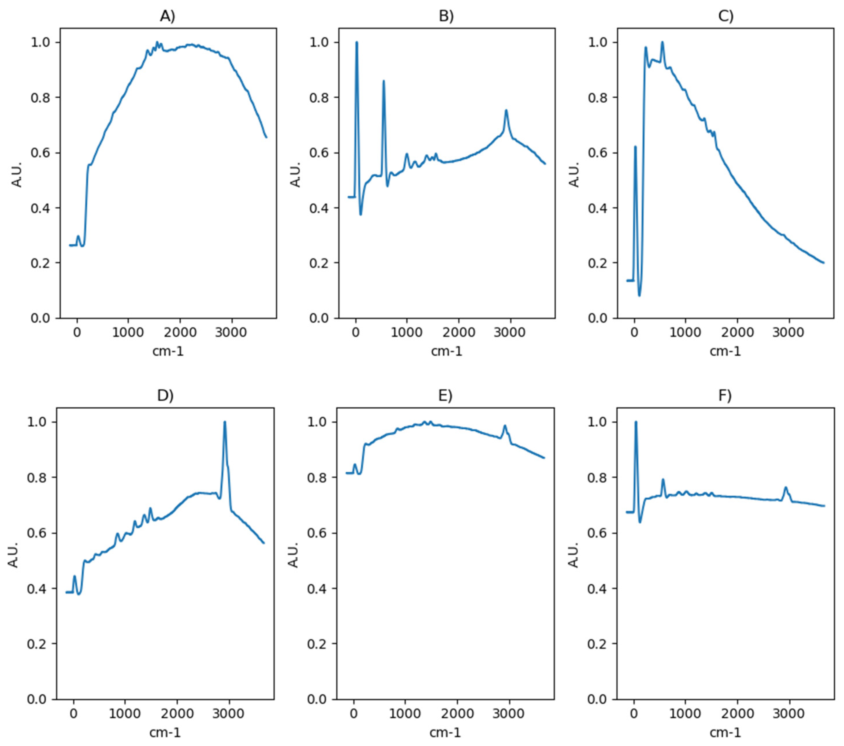
Examples of Raman spectra of marine water samples contaminated with ER (A–C) and PP (D–F), belonging to the MPDB database.
Figure 1.
Examples of Raman spectra of marine water samples contaminated with ER (A–C) and PP (D–F), belonging to the MPDB database.
Figure 2.
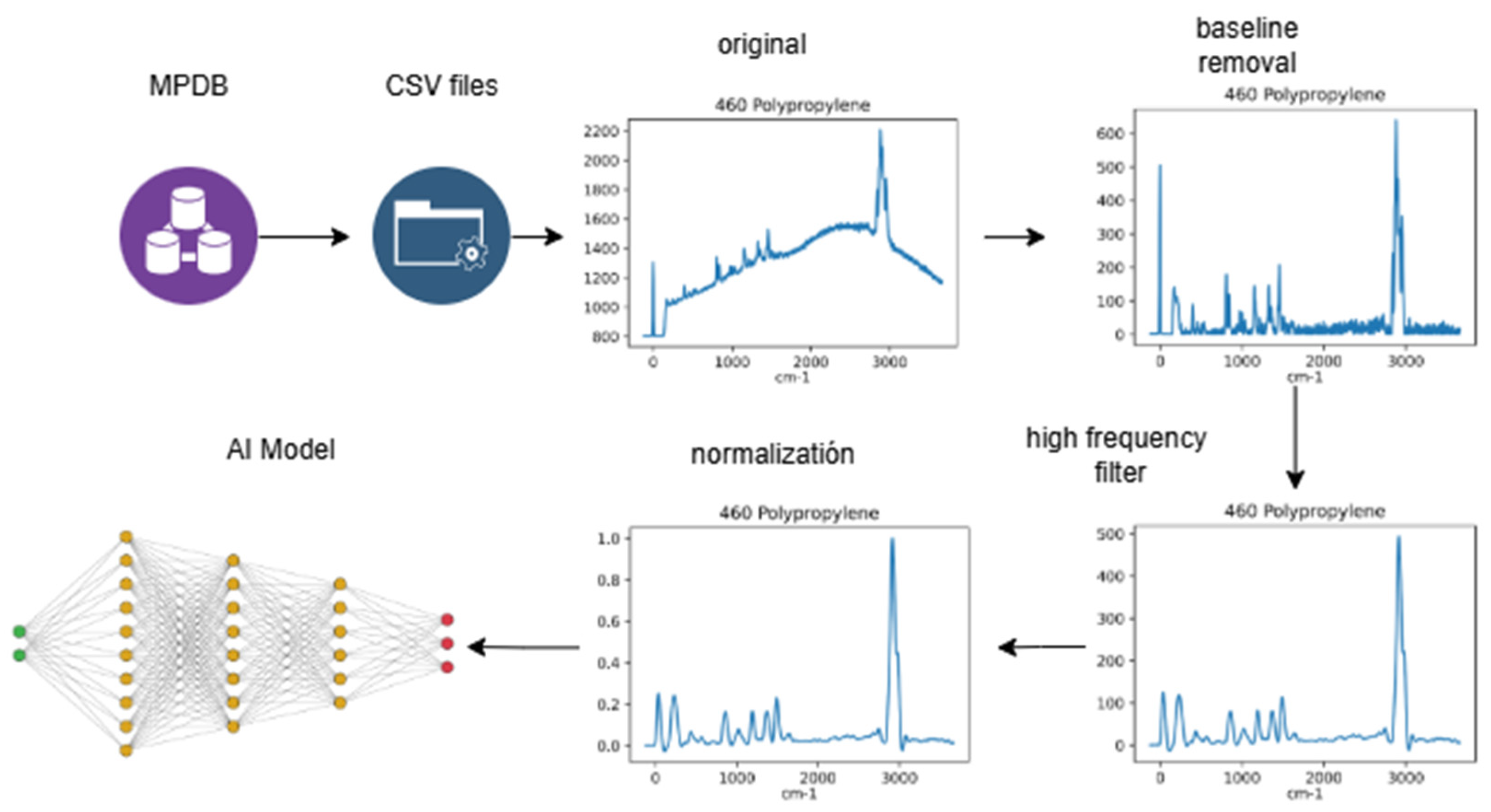
The figure shows the steps involved in typical preprocessing. The files containing the original Raman spectra are extracted from the MPDB, then the baseline is removed, followed by the elimination of high-frequency noise, and finally normalization is performed before feeding the data into the AI model.
Figure 2.
The figure shows the steps involved in typical preprocessing. The files containing the original Raman spectra are extracted from the MPDB, then the baseline is removed, followed by the elimination of high-frequency noise, and finally normalization is performed before feeding the data into the AI model.
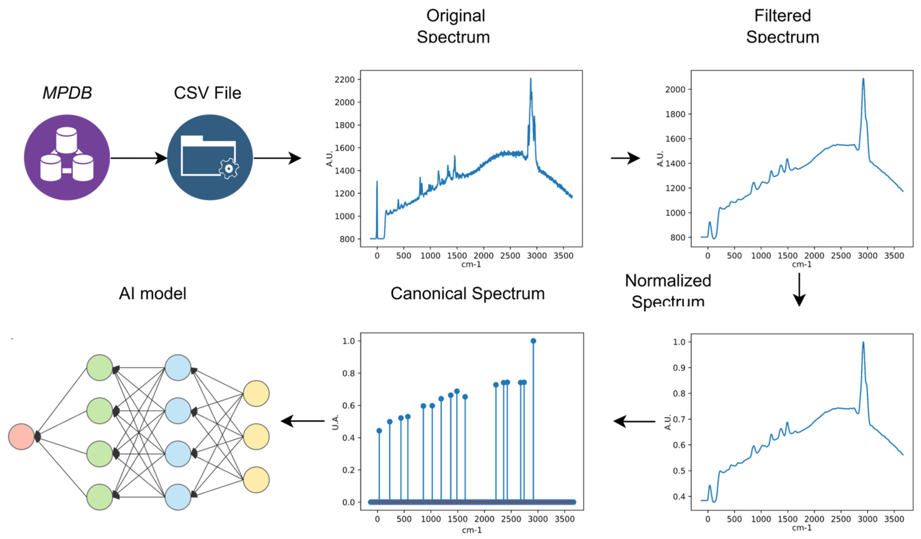
Figure 3.
The figure shows the stages that make up the CST. The files containing the original Raman spectra are extracted from the MPDB, followed by the elimination of high-frequency noise, then the normalization stage is carried out, and finally the canonical spectra is generated before feeding the data into the AI model.
Figure 3.
The figure shows the stages that make up the CST. The files containing the original Raman spectra are extracted from the MPDB, followed by the elimination of high-frequency noise, then the normalization stage is carried out, and finally the canonical spectra is generated before feeding the data into the AI model.
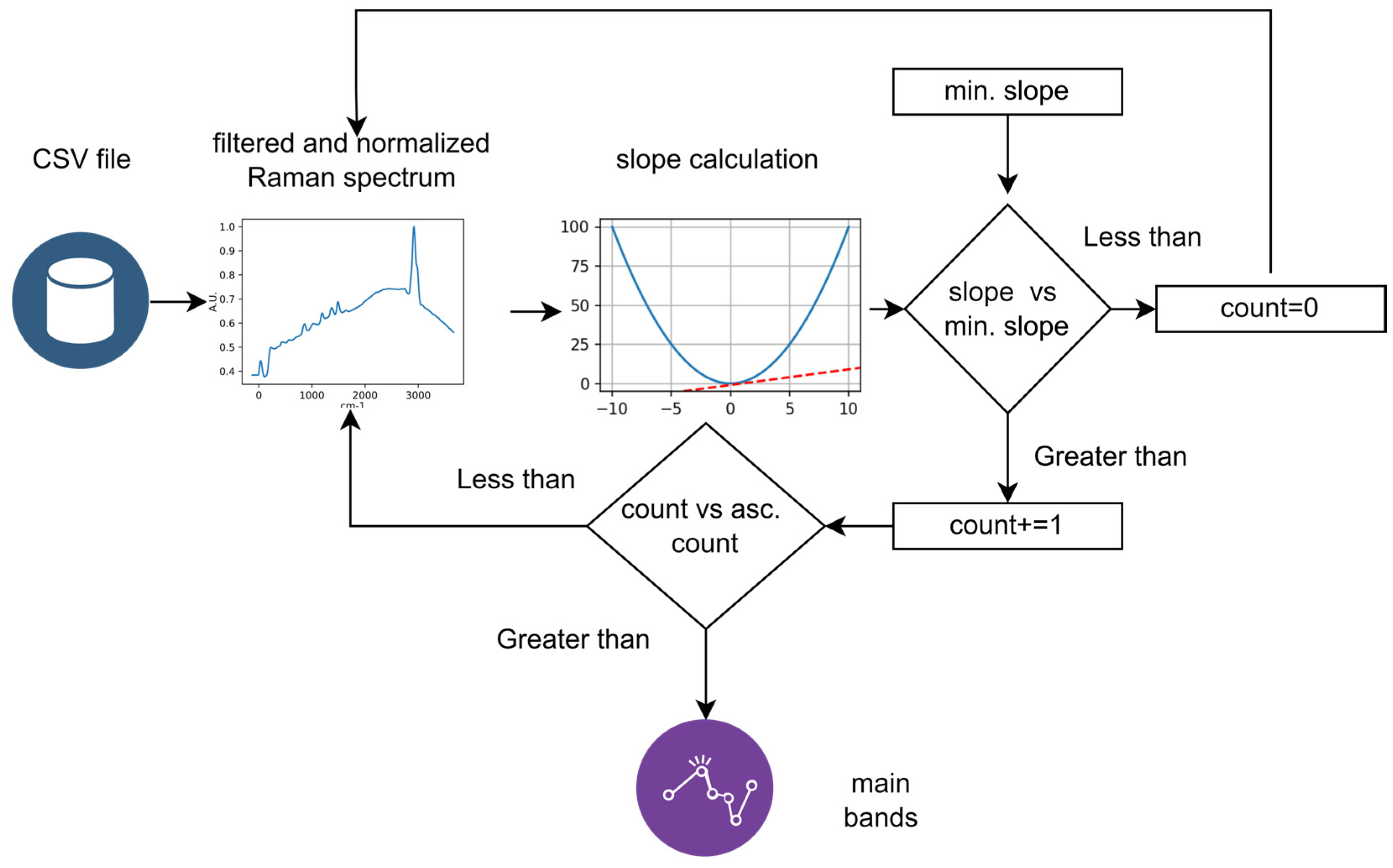
Figure 4.
Outline of the derivative-based algorithm used for detecting principal Raman bands, illustrating the evaluation of local slopes, threshold comparison, and identification of peak coordinates. A peak is only recorded if the signal shows a sustained positive slope (slope > min slope) for a minimum number of points count. This ensures that high-frequency noise, which can produce high instantaneous slopes, lacks spatial persistence and is effectively filtered out without the need for smoothing that could distort the peak’s position.
Figure 4.
Outline of the derivative-based algorithm used for detecting principal Raman bands, illustrating the evaluation of local slopes, threshold comparison, and identification of peak coordinates. A peak is only recorded if the signal shows a sustained positive slope (slope > min slope) for a minimum number of points count. This ensures that high-frequency noise, which can produce high instantaneous slopes, lacks spatial persistence and is effectively filtered out without the need for smoothing that could distort the peak’s position.
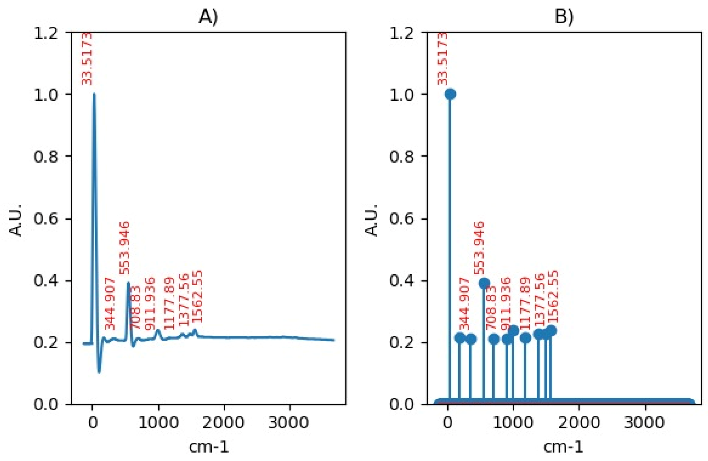
Figure 5.
Comparison of an original spectra (A) and a canonical spectra (B) for a sample of marine water contaminated with PB15, number 1441 in the MPDB Dataset.
Figure 5.
Comparison of an original spectra (A) and a canonical spectra (B) for a sample of marine water contaminated with PB15, number 1441 in the MPDB Dataset.
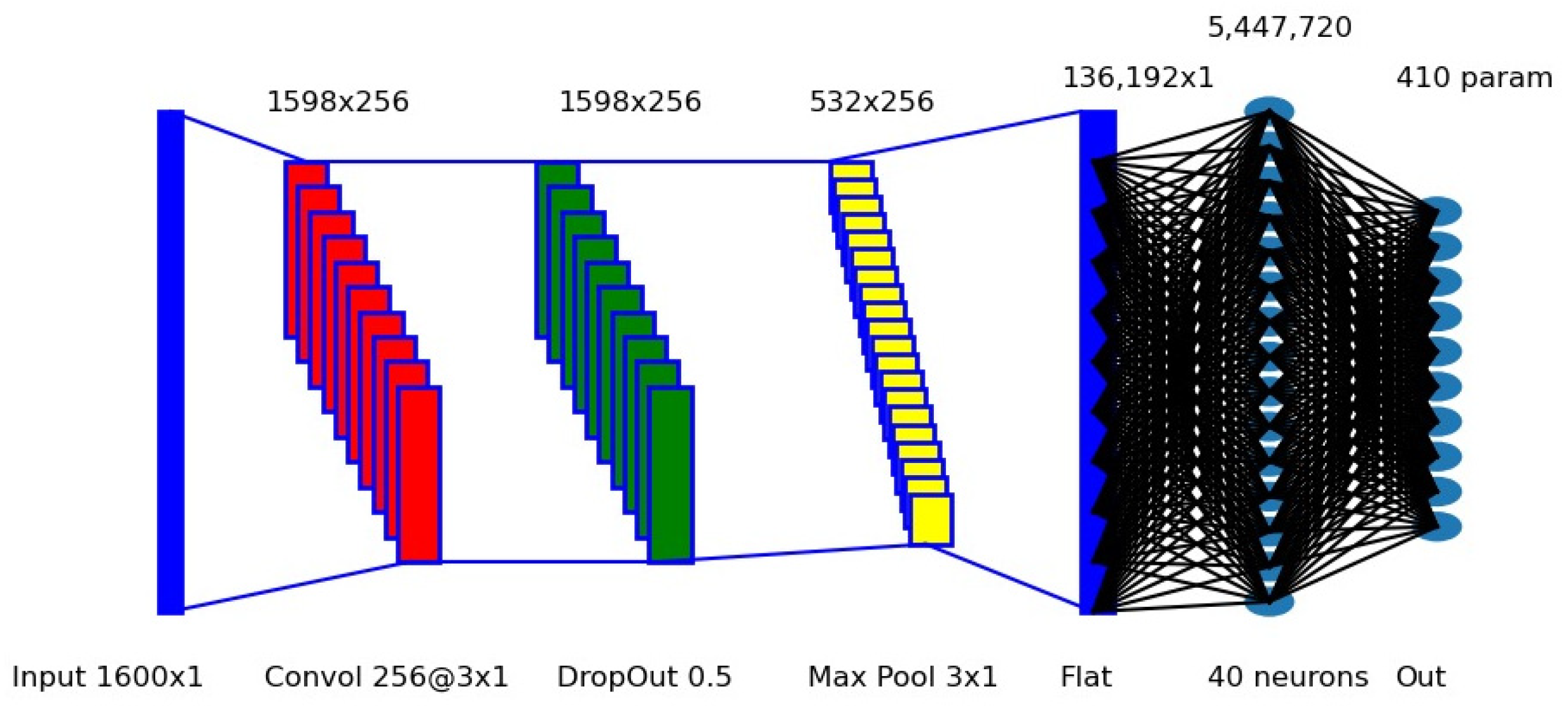
Figure 6.
Schematic representation of the CNN used for Raman-based microplastic classification, illustrating the convolution, dropout, pooling, flattening, and fully connected layers.
Figure 6.
Schematic representation of the CNN used for Raman-based microplastic classification, illustrating the convolution, dropout, pooling, flattening, and fully connected layers.
Figure 7.
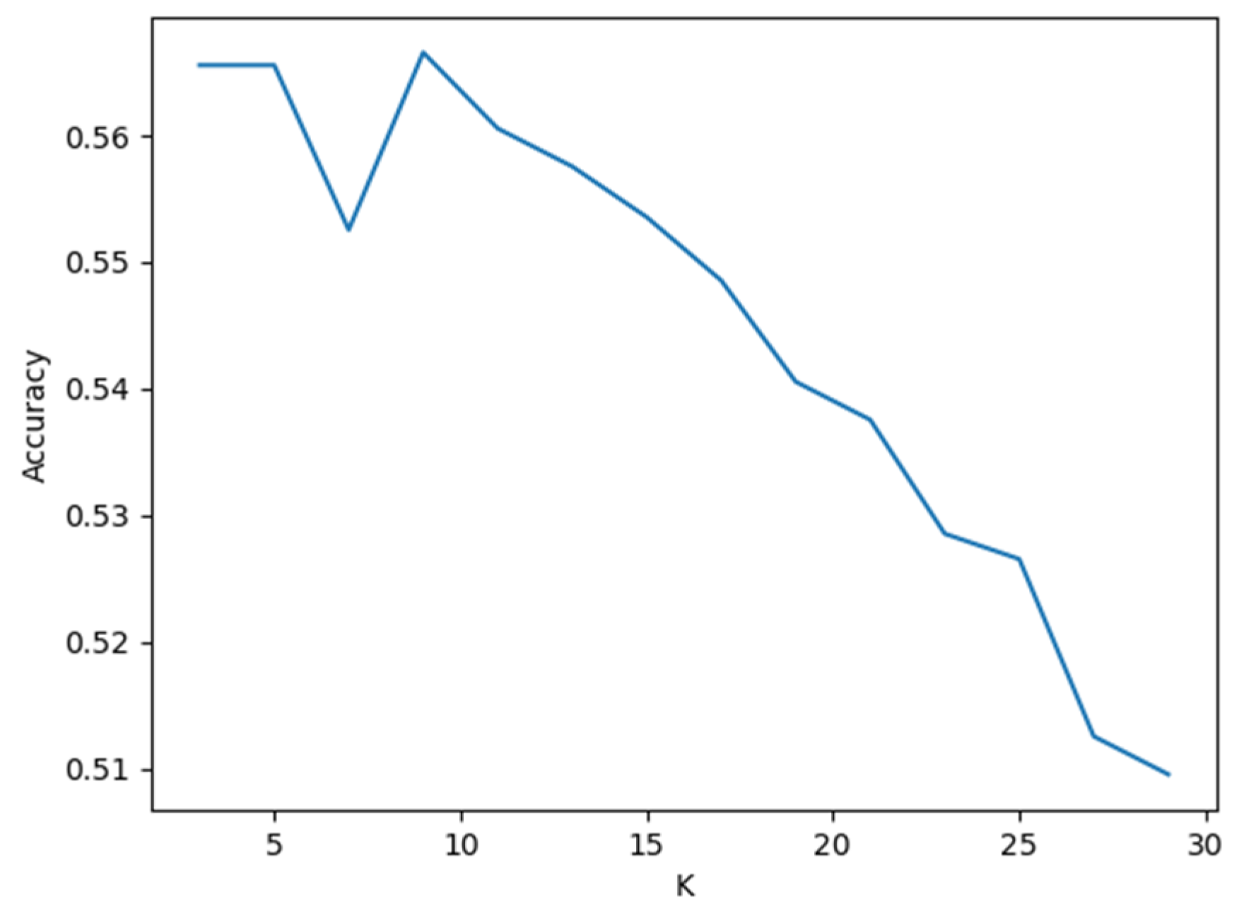
Estimation of optimal neighbor number (k) in the KNN model using typically preprocessed Raman spectra.
Figure 7.
Estimation of optimal neighbor number (k) in the KNN model using typically preprocessed Raman spectra.
Figure 8.
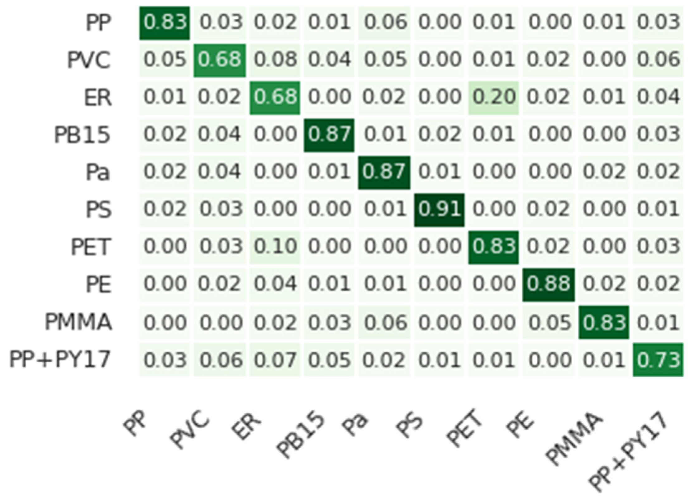
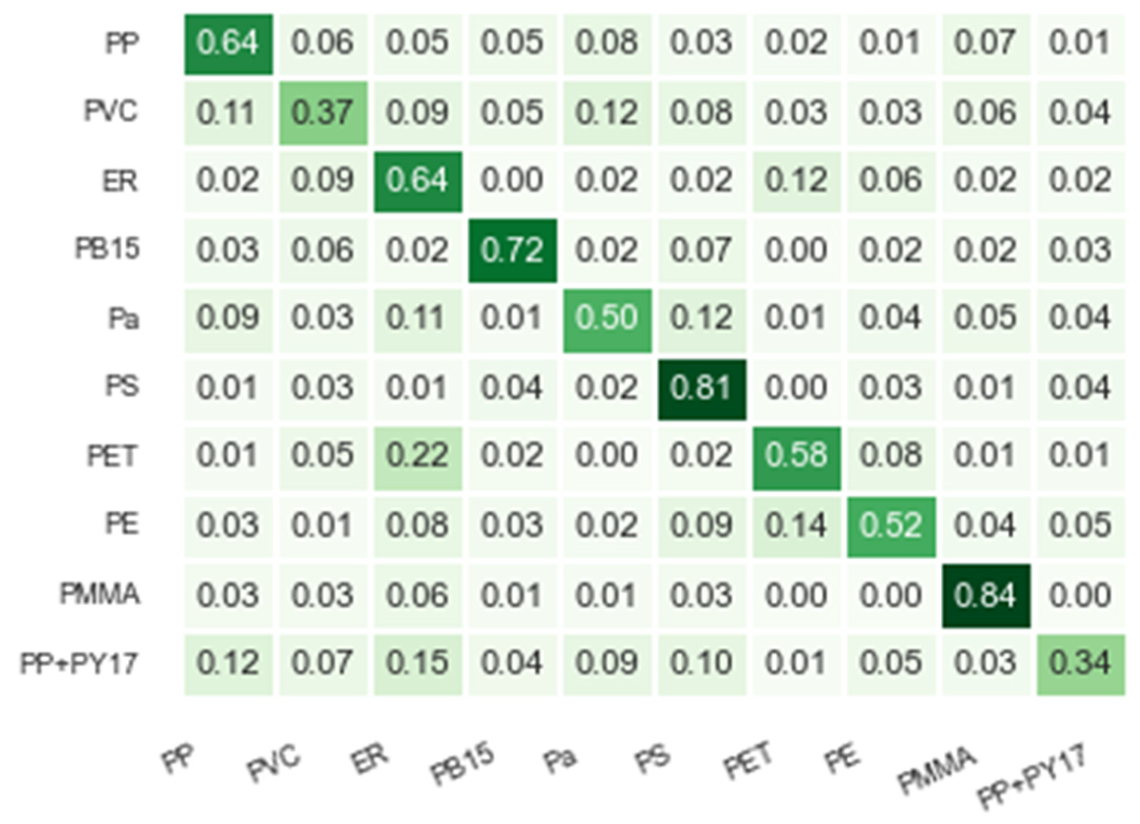
Confusion matrix for KNN classification using typical preprocessing.
Figure 8.
Confusion matrix for KNN classification using typical preprocessing.
Figure 9.
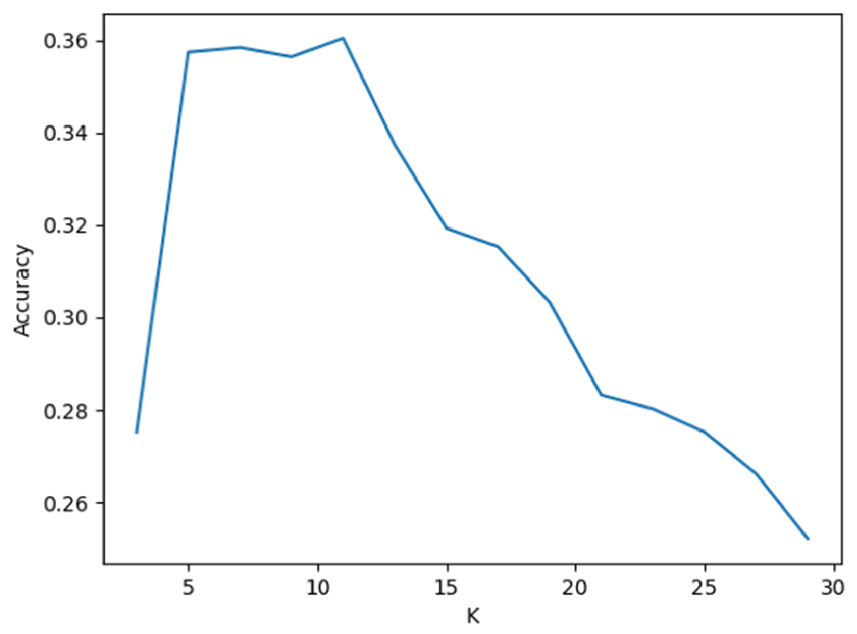
Estimation of optimal neighbor number (k) in the KNN model using CST.
Figure 9.
Estimation of optimal neighbor number (k) in the KNN model using CST.
Figure 10.
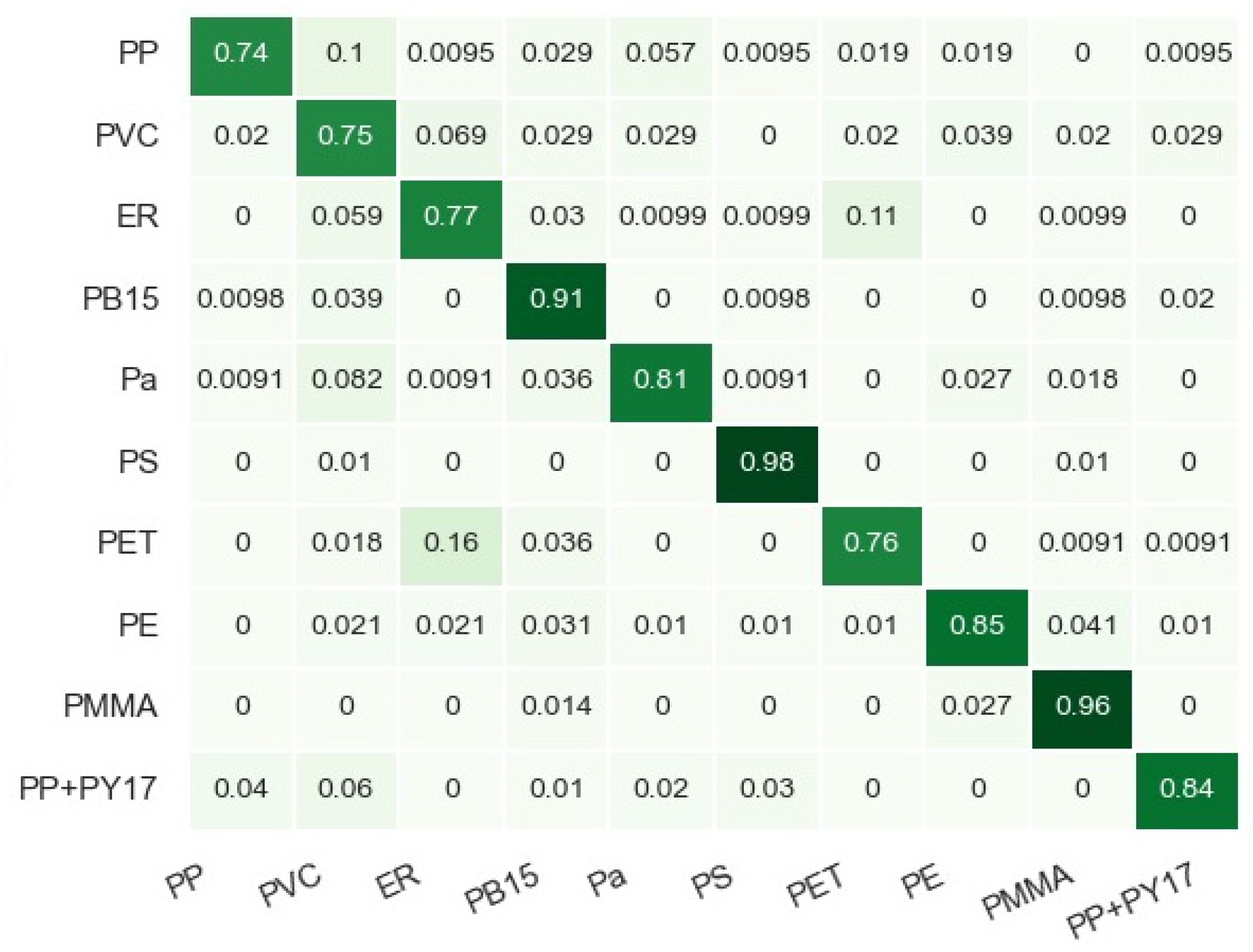
Confusion Matrix for KNN evaluating by CST using Raman spectra data.
Figure 10.
Confusion Matrix for KNN evaluating by CST using Raman spectra data.
Figure 11.
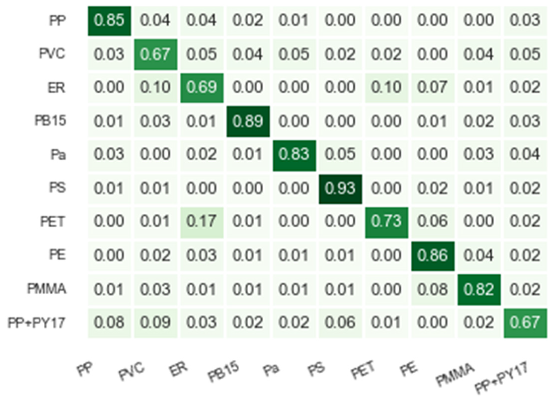
Confusion matrix for Random Forest classification using typical preprocessing.
Figure 11.
Confusion matrix for Random Forest classification using typical preprocessing.
Figure 12.
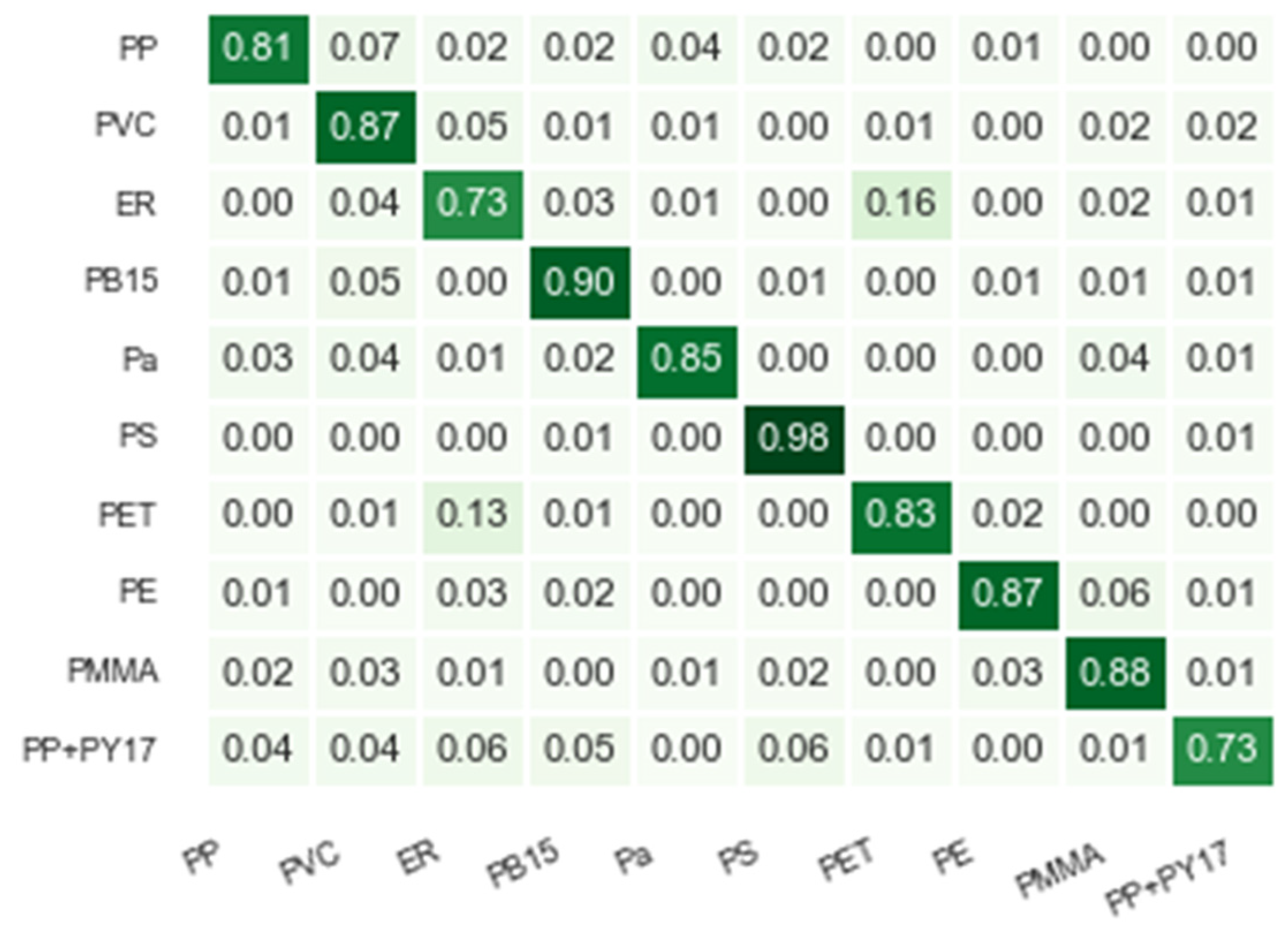
Confusion matrix for Random Forest classification by CST using Raman spectra data.
Figure 12.
Confusion matrix for Random Forest classification by CST using Raman spectra data.
Figure 13.
Confusion Matrix for XGBoost evaluating with typical sample preprocessing.
Figure 13.
Confusion Matrix for XGBoost evaluating with typical sample preprocessing.
Figure 14.
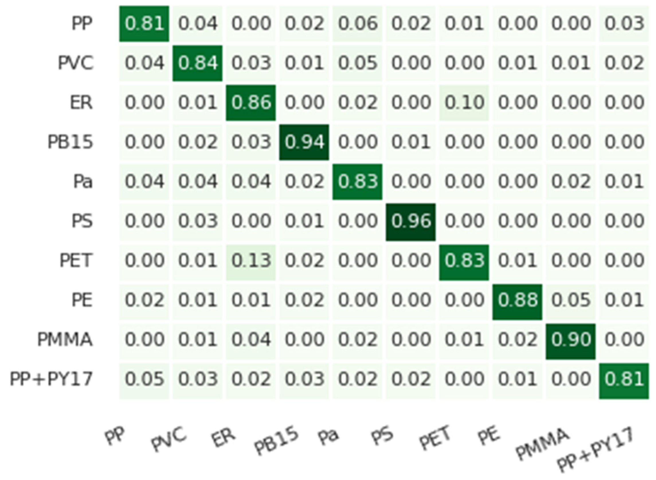
Confusion matrix for XGBoost classification by CST using Raman spectra data.
Figure 14.
Confusion matrix for XGBoost classification by CST using Raman spectra data.
Figure 15.
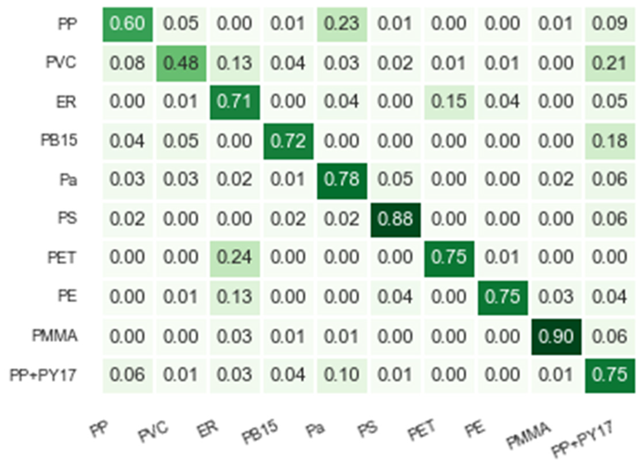
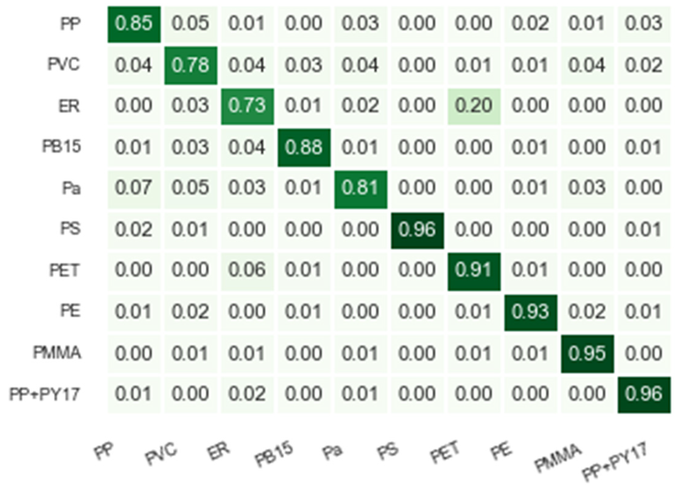
Confusion matrix for MLP by typical classification using Raman spectra data.
Figure 15.
Confusion matrix for MLP by typical classification using Raman spectra data.
Figure 16.
Confusion matrix for MLP classification by CST using Raman spectra data.
Figure 16.
Confusion matrix for MLP classification by CST using Raman spectra data.
Figure 17.
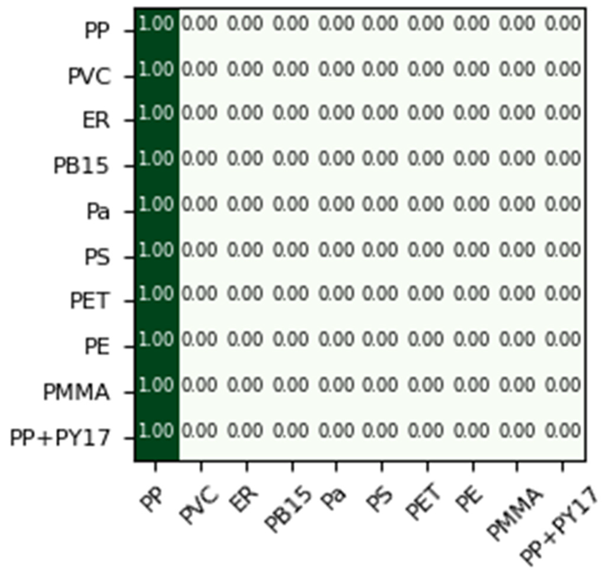
Confusion matrix for CNN by typical classification using Raman spectra data.
Figure 17.
Confusion matrix for CNN by typical classification using Raman spectra data.
Figure 18.
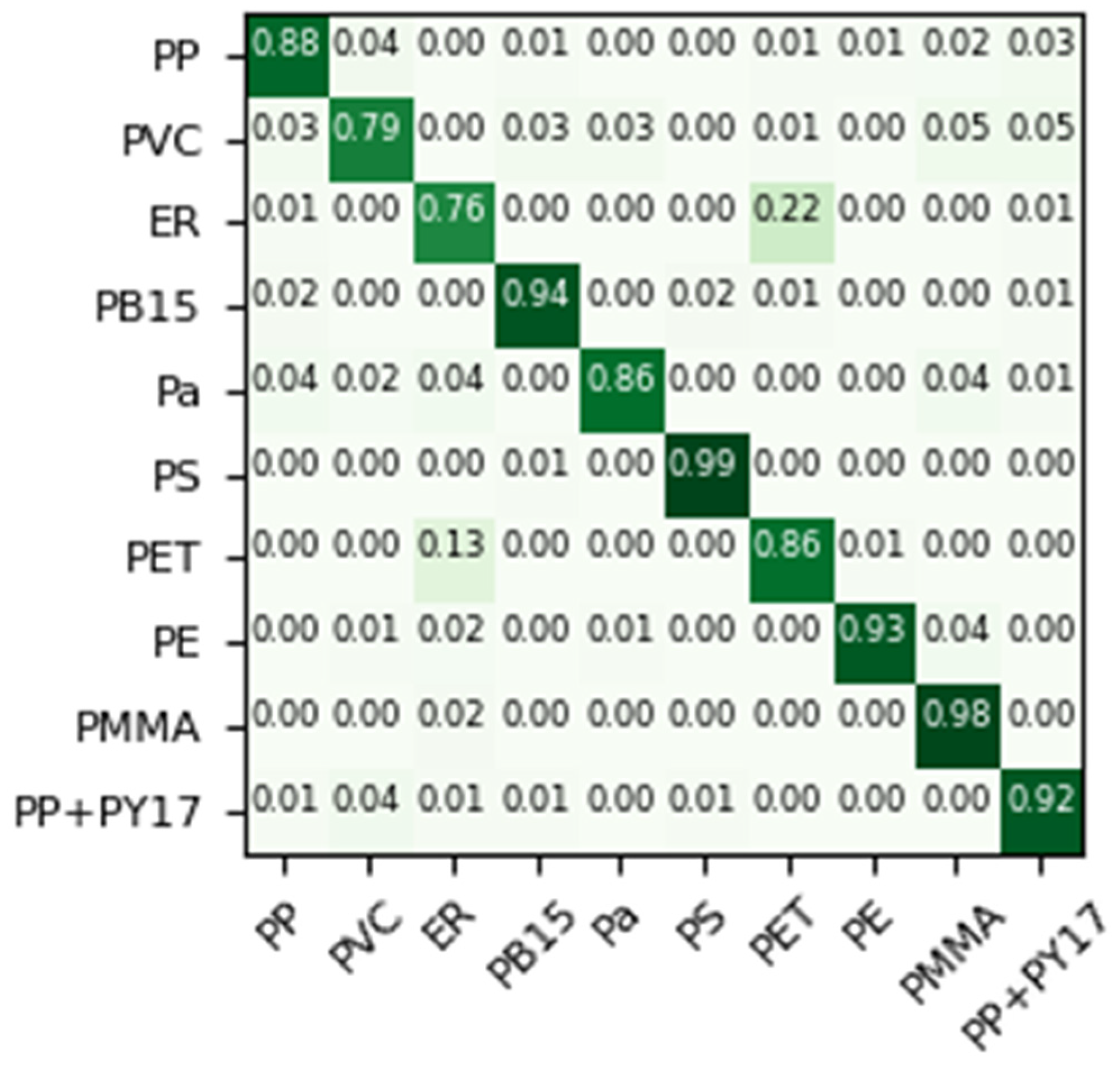
Confusion matrix for CNN by CST using Raman spectra data.
Figure 18.
Confusion matrix for CNN by CST using Raman spectra data.
Table 1.
Partial summary of polymer categories in the MPDB showing the number of Raman spectra available for each microplastic type.
Table 1.
Partial summary of polymer categories in the MPDB showing the number of Raman spectra available for each microplastic type.
| Microplastic Type | Acronym | Number of Samples |
|---|
| Poly(ethylene terephthalate) | PET | 21,769 |
| Poly(tetrafluoroethylene) | PTFE | 17,284 |
| Polypropylene | PP | 14,613 |
| Polyethylene | PE | 4972 |
| Polystyrene | PS | 4001 |
| Poly(vinyl chloride) | PVC | 3235 |
| Phthalocyanine Blue | PB15 | 2120 |
| Parafilm | Pa | 864 |
| Poly(methyl methacrylate) | PMMA | 808 |
| Epoxy resin1 | ER | 655 |
| Polypropylene + PY17based | PP+PY17 | 561 |
Table 2.
Python libraries were used for data processing and model development in this study.
Table 2.
Python libraries were used for data processing and model development in this study.
| Library | Application |
|---|
| keras v.2.12.0 | API deep learning |
| Pandas v.2.0.3 | Data management and csv |
| Matplotlib v.3.7.2 | Graphics generator |
| Numpy v.1.24.3 | Numerical computing |
| Sklearn v.1.3.0 | Data analysis |
| Tensorflow v.2.12.1 | Low level API Deep learning |
Table 3.
Summarizes the parameter space explored during KNN training for microplastic classification.
Table 3.
Summarizes the parameter space explored during KNN training for microplastic classification.
| Parameter | Values |
|---|
| neighbors (k) | 5, 7 |
| weights | Distance |
| p | 1, 2 |
| metric | Minkowski, Mahalanobis, Seuclidean, Euclidean, Manhattan |
Table 4.
The ranges of hyperparameters evaluated during RF training for MPs identification using Raman spectral data are shown.
Table 4.
The ranges of hyperparameters evaluated during RF training for MPs identification using Raman spectral data are shown.
| Parameter | Values |
|---|
| max_depth | 3, 5, 7, 10 |
| n_estimators | 100, 200, 300, 400, 500 |
| max_features | 10, 20, 30, 40 |
| min_samples_leaf | 1, 2, 4 |
Table 5.
Parameter space used for training the MLP model for microplastic classification.
Table 5.
Parameter space used for training the MLP model for microplastic classification.
| Parameter | Values |
|---|
| hidden_layer_sizes | (10,20,10), (15,20,20), (30,20,30) |
| activation | Tanh, ReLU |
| solver | SGD, Adam |
| alpha | 0.0001, 0.05 |
| learning rate | constant, adaptive |
Table 6.
Parameters used for training the XGBoost model for MPs classification.
Table 6.
Parameters used for training the XGBoost model for MPs classification.
| Parameter | Values |
|---|
| Booster | gbtree, gblinear, dart |
| subsample | 0.2, 1.0 |
| Eta | 0.1, 1.0 |
| colsample bytree | 0.2, 1.0 |
Table 7.
Parameter space used for training the CNN model for microplastic classification.
Table 7.
Parameter space used for training the CNN model for microplastic classification.
| Parameter | Values |
|---|
| Weight constraint | 1, 3, 5 |
| Dropout rate | 0.1, 0.4, 0.9 |
| Fully connected layers | 30, (30,30), 60 |
Table 8.
Performance metrics obtained for the five AI models using typical and CST strategies.
Table 8.
Performance metrics obtained for the five AI models using typical and CST strategies.
| Model | Pre Processing | Precision | Recall | F1-Score | Accuracy |
|---|
| KNN | Typical | 0.74 | 0.73 | 0.73 | 0.73 |
| KNN | Canonical | 0.83 | 0.83 | 0.83 | 0.83 |
| RF | Typical | 0.74 | 0.73 | 0.73 | 0.73 |
| RF | Canonical | 0.83 | 0.83 | 0.83 | 0.83 |
| XGBoost | Typical | 0.80 | 0.81 | 0.80 | 0.80 |
| XGBoost | Canonical | 0.85 | 0.85 | 0.85 | 0.84 |
| MLP | Typical | 0.78 | 0.77 | 0.77 | 0.77 |
| MLP | Canonical | 0.87 | 0.87 | 0.87 | 0.88 |
| CNN | Typical | 0.01 | 0.10 | 0.02 | 0.10 |
| CNN | Canonical | 0.90 | 0.90 | 0.90 | 0.90 |
Table 9.
Statistical test by Wilcoxon using 10 folds and accuracy value.
Table 9.
Statistical test by Wilcoxon using 10 folds and accuracy value.
| Model | KNN | MLP | XGBoost | RF | CNN |
|---|
| p-value | 0.00296 | 0.00296 | 0.00296 | 0.00296 | 0.00296 |
| Median Can-Typ > 0 | 0.045 | 0.174 | 0.0425 | 0.1975 | 0.86755 |
Table 10.
Regarding the Wilcoxon statistical test to determine which classifier model performs best using CST approach, the same alternative hypothesis H1 is used again. The table shows the p-values for each comparison between models. It can be observed that the KNN classifier performed the worst, as the p-value for each comparison was less than the significance level of 0.05 (all p > 0.05). For the MLP classifier, its performance is better than the KNN (p = 0.003), XGBoost (p = 0.011), and Rf (p = 0.003) classifiers; however, it is not significantly better than the CNN classifier (p > 0.05). Regarding the CNN classifier, the p-value is less than the significance level of 0.05 in all cases, indicating that it is the model that performed best using the CST approach. Finally, we observed that the RF and XGBoost classifiers are mid-performance models that fall short of the performance of MLP and CNN.
Table 10.
Regarding the Wilcoxon statistical test to determine which classifier model performs best using CST approach, the same alternative hypothesis H1 is used again. The table shows the p-values for each comparison between models. It can be observed that the KNN classifier performed the worst, as the p-value for each comparison was less than the significance level of 0.05 (all p > 0.05). For the MLP classifier, its performance is better than the KNN (p = 0.003), XGBoost (p = 0.011), and Rf (p = 0.003) classifiers; however, it is not significantly better than the CNN classifier (p > 0.05). Regarding the CNN classifier, the p-value is less than the significance level of 0.05 in all cases, indicating that it is the model that performed best using the CST approach. Finally, we observed that the RF and XGBoost classifiers are mid-performance models that fall short of the performance of MLP and CNN.
| Model | KNN | MLP | XGBoost | RF | CNN |
|---|
| KNN | - | 0.998 | 0.998 | 0.998 | 0.998 |
| MLP | 0.003 | - | 0.011 | 0.003 | 0.998 |
| XGBoost | 0.003 | 0.992 | - | 0.003 | 0.998 |
| RF | 0.003 | 0.998 | 0.998 | - | 0.998 |
| CNN | 0.003 | 0.003 | 0.003 | 0.003 | - |
Table 11.
Summary of results. In blue, the greatest increase in the ranking of MPs according to the AI model is shown, while the best-ranked MP of each model is highlighted in bold.
Table 11.
Summary of results. In blue, the greatest increase in the ranking of MPs according to the AI model is shown, while the best-ranked MP of each model is highlighted in bold.
| MP | KNN | RF | XGBoost | MLP | CNN |
|---|
| Typ | Can | Typ | Can | Typ | Can | Typ | Can | Typ | Can |
|---|
| PP | 0.64 | 0.74 | 0.85 | 0.81 | 0.83 | 0.81 | 0.60 | 0.91 | 1.00 | 0.88 |
| PVC | 0.37 | 0.75 | 0.67 | 0.87 | 0.68 | 0.84 | 0.48 | 0.82 | 0.00 | 0.79 |
| ER | 0.64 | 0.77 | 0.69 | 0.73 | 0.68 | 0.86 | 0.71 | 0.80 | 0.00 | 0.76 |
| PB15 | 0.72 | 0.91 | 0.89 | 0.90 | 0.87 | 0.94 | 0.72 | 0.91 | 0.00 | 0.94 |
| Pa | 0.50 | 0.81 | 0.83 | 0.85 | 0.87 | 0.83 | 0.78 | 0.87 | 0.00 | 0.86 |
| PS | 0.81 | 0.98 | 0.93 | 0.98 | 0.91 | 0.96 | 0.88 | 0.97 | 0.00 | 0.99 |
| PET | 0.58 | 0.76 | 0.73 | 0.83 | 0.83 | 0.83 | 0.75 | 0.88 | 0.00 | 0.86 |
| PE | 0.84 | 0.85 | 0.86 | 0.87 | 0.88 | 0.88 | 0.75 | 0.96 | 0.00 | 0.93 |
| PMMA | 0.34 | 0.96 | 0.82 | 0.88 | 0.83 | 0.90 | 0.90 | 0.95 | 0.00 | 0.98 |
| PP+PY17 | 0.63 | 0.84 | 0.67 | 0.73 | 0.73 | 0.81 | 0.75 | 0.85 | 0.00 | 0.92 |
Maximum
True Prediction | 38% | 20% | 18% | 34% | 99% |
Table 12.
Interference matrix of the analyzed polymers. Yellow cells represent the highest-intensity Raman bands; green cells indicate secondary intensities. Column headers specify the vibrational mode associated with each band.
Table 12.
Interference matrix of the analyzed polymers. Yellow cells represent the highest-intensity Raman bands; green cells indicate secondary intensities. Column headers specify the vibrational mode associated with each band.
| MP | C–C | C–C | CF3 | C–F | C–O–C | RING
Breath | CH | C–C | CH2 | CH2 | RING Stretch | RING Stretch | ESTE | CH2 | CH2 |
|---|
| PS | | | | | | 1001 | 1031 | | | | | 1602 | | 2900 | 3050 |
| PE | | | | | | | 1062 | 1130 | 1296 | 1417 | | | | 2850 | |
| PET | | 630 | | | 856 | | | | 1308 | | | 1615 | 1726 | | |
| PP | | | | | 832 | 967 | | 1150 | 1324 | 1454 | | | | 2800 | 2950 |
| PVC | 361 | 636 | 694 | | | | | | 1330 | 1430 | | 1590 | | 2916 | 2940 |
| PB15 | | | 680 | 747 | | | | 1142 | 1340 | | 1529 | | | | |
| ER | | | | | 826 | | | 1116 | 1240 | | | 1585 | | 2920 | 3071 |
| Pa | | | | | 814 | | | | | 1455 | | | 1730 | 2954 | |
| PMMA | | | | | 829 | 986 | | | | 1451 | | | 1725 | 2945 | 2994 |
| PP+PY | | | | | | | | | | 1443 | | 1629 | | 2916 | |
Table 13.
The interference matrix shows the Raman frequency bands associated with each pair of MPs analyzed [
33]. The cells highlighted in yellow indicate the bands with the highest intensity, while the cells highlighted in green denote the bands with the second highest intensity. These bands reflect the vibrational modes that are most likely to contribute to spectral overlap and, consequently, to false negative classifications in the different models.
Table 13.
The interference matrix shows the Raman frequency bands associated with each pair of MPs analyzed [
33]. The cells highlighted in yellow indicate the bands with the highest intensity, while the cells highlighted in green denote the bands with the second highest intensity. These bands reflect the vibrational modes that are most likely to contribute to spectral overlap and, consequently, to false negative classifications in the different models.
| Plastic 1 | Plastic 2 | Freq (cm−1) | Freq (cm−1) |
|---|
| PP | Pa | 814, 832 | 1454, 1455 |
| PB15 | PS | x | x |
| ER | PET | 856, 826 | x |
| PMMA | PE | 1417, 1451 | 2850, 2945 |
| ER | PMMA | 826, 829 | 2945, 2920 |
| PP | PP+PY | 1443, 1454 | 2800, 2916 |
| PVC | PP | 1324, 1330 | 2950, 2940 |
| Pa | PVC | 2916, 2954 | 1430, 1455 |
| PET | ER | 826, 856 | 585, 1615 |
| ER | PB15 | 1142, 1116 | 1240, 1340 |




 ,
,