Control-Enhanced Hamiltonian Optimization for Quantum Parameter Estimation in Many-Body Systems

Abstract

Quantum metrology uses the principles of quantum mechanics to improve the accuracy of parameter estimation so that it can surpass the classical limit. However, noise and the challenge of preparing multipartite entangled states hinder practical applications. In this work, we use the Lipkin-Meshkov-Glick model as the experimental platform and the quantum parameter estimation package QuanEstimation as a tool to improve the quantum parameter estimation in many-body systems by using Hamiltonian control optimization. We apply auto-GRAPE, PSO, and DE algorithm to optimize the time-dependent control field. Our results show that the optimal control strategy can significantly enhance the quantum Fisher information and reduce the quantum Cramér-Rao bound even under environmental noise. These findings provide a way to achieve the parameter estimation limit in a noisy environment and promote the development of practical quantum metrology applications.

1. Introduction

Quantum metrology, which uses fundamental quantum principles to achieve precision beyond classical limits, has attracted substantial research interest in recent years [1,2,3,4,5,6,7,8,9,10,11,12]. By exploiting nonclassical resources such as entanglement and spin squeezing, this emerging field demonstrates unprecedented accuracy in parameter estimation tasks, particularly in scenarios involving quantum-enhanced measurement protocols [13,14,15] and multi-particle entangled states [16,17]. The theoretical framework builds upon Heisenberg uncertainty principle and quantum superposition effects, enabling measurement sensitivities approaching the fundamental bounds dictated by quantum mechanics [18,19,20,21,22].

The quantum Cramér-Rao bound (QCRB) [22,23,24] sets the fundamental precision limit, indicating that the uncertainty in estimating parameters $\overrightarrow{\theta }$ contained in a quantum state $\rho (\overrightarrow{\theta })$ is inversely proportional to the square root of the quantum Fisher information matrix (QFIM), expressed as ${\Delta }^2\overrightarrow{\theta }\ge 1/\mathcal{F}$ [1,25,26,27,28,29]. Collective interactions in many-body systems lead to increased sensitivity, especially near quantum critical points, where the QFIM scales superlinearly due to divergent susceptibility [30,31,32,33]. The Lipkin-Meshkov-Glick (LMG) model, involving N spins with infinite-range interactions, is an exemplary system for studying quantum-enhanced sensing driven by criticality [34,35,36]. Nonetheless, significant challenges persist in translating these theoretical benefits into practical applications.

The preparation and maintenance of multipartite entangled states [37,38], a prerequisite for surpassing standard quantum limits, face technical bottlenecks in realistic noisy environments. Moreover, sensitivity enhancement near critical points often comes at the cost of reduced dynamic stability and increased susceptibility to parameter fluctuations [39,40,41,42,43]. Hamiltonian optimization emerges as a promising pathway to address these limitations [8,9,10,44,45,46,47,48], where optimized interaction design enables both rapid entanglement generation and inherent noise resilience.

Recent advancements have shown that by employing controlled LMG-type Hamiltonians along with time-reversal procedures, it is possible to reduce phase decoherence while retaining metrological benefits [49]. Additionally, non-Hermitian systems featuring parity-time symmetry offer novel pathways for enhancing sensing through engineering exceptional points, although challenges persist in achieving precise control of Hamiltonians at the quantum level [50,51,52]. These progressions underscore the delicate equilibrium necessary between Hamiltonian intricacy, utilization of quantum resources, and suppression of environmental noise, representing a frontier that necessitates interdisciplinary approaches merging quantum control theory, open system dynamics, and critical phenomenon analysis.

In this work, we suggest utilizing quantum control optimization techniques, specifically gradient ascent pulse engineering (GRAPE) [8,9,53,54] that leverage automatic differentiation (AD) and differential evolution (DE) [53], in conjunction with machine learning-enhanced particle swarm optimization (PSO) algorithms [44], to create control strategies that go beyond the usual precision limits in quantum parameter estimation. These methods allow for the automated generation of optimal control sequences that push the boundaries of metrological precision in various quantum dynamical systems, while also accommodating real-world experimental limitations. Hence, this framework establishes a comprehensive method for devising controlled quantum metrological approaches. Through computational simulations, we illustrate that the optimized control strategies achieve parameter estimation precision that exceeds the fundamental limits imposed by the coherence time of the system, a significant departure from traditional approaches where precision boundaries are universally restricted by coherence duration.

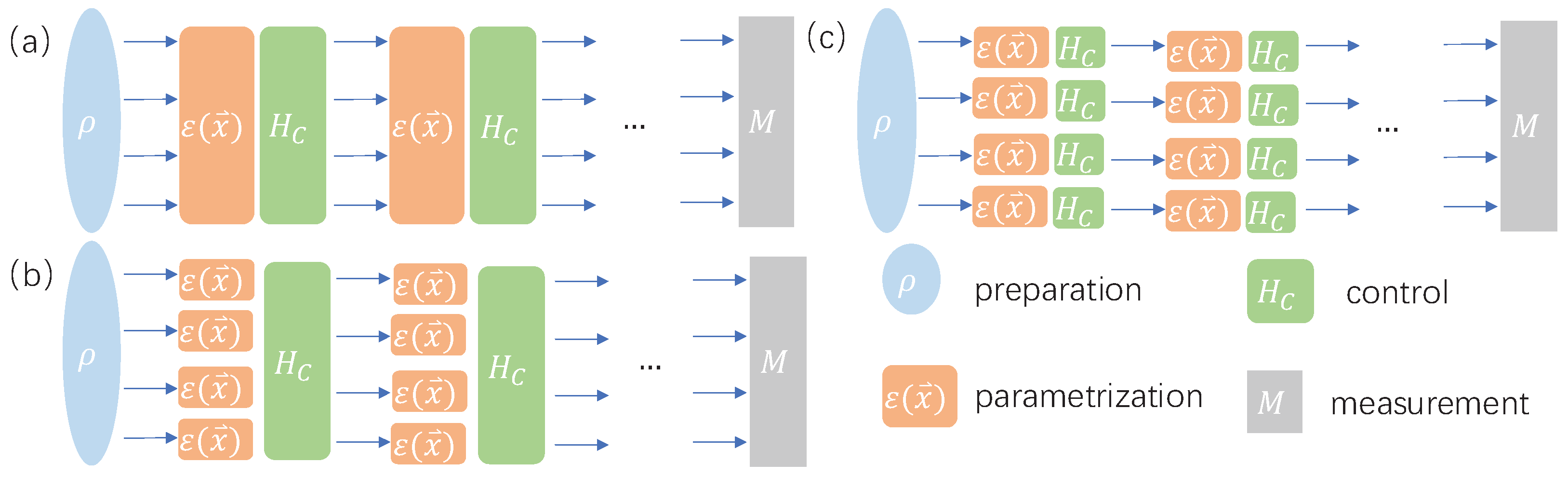
This study addresses the gap by merging the essential characteristics of the many-body quantum model with numerical optimization using Hamiltonian optimal control techniques from the QuanEstimation package [53,55]. This integration allows for a methodical investigation of control tactics for parameter estimation. Hamiltonian control optimization, as shown in Figure 1, which involves creating time-dependent fields to direct quantum dynamics [8], has proven to be a valuable approach in maximizing $\mathcal{F}$.

The structure of this document is organized as follows. Section 2 introduces essential theoretical concepts in quantum parameter estimation, such as the QFIM and the QCRB. And the LMG model and its dynamic evolution process are presented. Our proposed control Hamiltonian optimization scheme is detailed in Section 3. Section 4 showcases numerical simulation results that illustrate the quantum advantage in parameter sensitivity and resilience to noise using the QuanEstimation package. Finally, Section 5 summarizes the main findings and discusses the implications for quantum metrology applications.

2. Background

2.1. Quantum Parameter Estimation

In the case of a general quantum state $\rho \left(\overrightarrow{x}\right)$ that encodes parameters $\overrightarrow{x}=\{x_1,x_2,\dots \}$ through unitary dynamics $U\left(\overrightarrow{x}\right)=e^{-iH\left(\overrightarrow{x}\right)t}$ or the noise dynamics ${\mathsf{\partial }}_t\rho =-i[H\left(\overrightarrow{x}\right),\rho \left(\overrightarrow{x}\right)]+\mathcal{L}\left(t\right)$, where $\mathcal{L}\left(t\right)$ are the superoperators, the elements of the QFIM are determined by the symmetric logarithmic derivative (SLD) as follows:

$${\mathcal{F}}_{ij}={\displaystyle \frac{1}{2}}\mathrm{Tr}\left[\rho \{L_i,L_j\}\right],$$

(1)

where the SLD operators $L_i$ satisfy the implicit equation ${\mathsf{\partial }}_i\rho ={\displaystyle \frac{1}{2}}(\rho L_i+L_i\rho )$. The diagonal elements ${\mathcal{F}}_{ii}$ provide the single-parameter quantum Fisher information (QFI).

In the scenario of pure states $\rho =|\psi \rangle \langle \psi |$, this framework simplifies to $L_i=2\left(\right|{\mathsf{\partial }}_i\psi \rangle \langle \psi |+|\psi \rangle \langle {\mathsf{\partial }}_i\psi \left|\right)$, facilitating the explicit computation of QFIM via state overlaps. For mixed states, the spectral decomposition $\rho ={\sum }_k{\lambda }_k|k\rangle \langle k|$ offers an alternate representation, where

$${\mathcal{F}}_{ij}=\sum _{k,l}{\displaystyle \frac{{({\lambda }_k-{\lambda }_l)}^2}{{\lambda }_k+{\lambda }_l}}\mathrm{Re}[\langle k|{\mathsf{\partial }}_i\rho |l\rangle \langle l|{\mathsf{\partial }}_j\rho |k\rangle ].$$

(2)

The QFIM plays a crucial role in quantum multiparameter estimation theory by setting the ultimate precision limit using the QCRB. The QCRB sets a lower boundary on the covariance matrix of any unbiased estimator, dictated by the QFIM. The QCRB is expressed as:

$$Cov[\widehat{\overrightarrow{x}}]\ge {\displaystyle \frac{1}{n}}\mathcal{F}{\left(\overrightarrow{x}\right)}^{-1}\ge {\displaystyle \frac{1}{n}}{I}_{\mathcal{M}}{\left(\overrightarrow{x}\right)}^{-1},$$

(3)

where $Cov[\widehat{\overrightarrow{x}}]$ represents the covariance matrix of the estimator, $\mathcal{F}\left(\overrightarrow{x}\right)$ signifies the QFIM, and $I_{\mathcal{M}}\left(\overrightarrow{x}\right)$ represents the classical Fisher information matrix. The classical Fisher information matrix is defined as:

$${\left[I_{\mathcal{M}}\right]}_{ij}=\sum _{k=1}^n{\displaystyle \frac{1}{p_k\left(\mathit{\theta }\right)}}{\displaystyle \frac{\mathsf{\partial }{p}_k\left(y\right|\overrightarrow{x})}{\mathsf{\partial }{x}_i}}{\displaystyle \frac{\mathsf{\partial }{p}_k\left(y\right|\overrightarrow{x})}{\mathsf{\partial }{x}_j}},$$

(4)

where $\mathrm{Cov}\left(\overrightarrow{x}\right)$ represents the covariance matrix of estimated parameters $\overrightarrow{x}$, and $\mathcal{F}$ denotes the QFIM, and n is the number of experiments. $p_k\left(y\right|\overrightarrow{x})$ denotes the probability of observing the k-th outcome of a measurement y, and $\mathcal{M}$ represents the measurement operators $\mathcal{M}=\left\{{\mathrm{\Pi }}_y\right\}$. This QFIM aids in determining the optimal measurement strategy and the fundamental precision limits in quantum metrology.

In quantum parameter estimation, the Holevo Cramér-Rao bound (HCRB) serves as a valuable asymptotic bound, typically tighter than the QCRB [56]. The HCRB is formulated as

$$\mathrm{Tr}(W\mathrm{cov}(\widehat{\overrightarrow{x}},\{{\mathrm{\Pi }}_y\}))\ge \underset{\overrightarrow{X},V}{min}\mathrm{Tr}\left(WV\right),$$

(5)

where W denotes the weight matrix, and V is a matrix satisfying $V\ge Z\left(\overrightarrow{X}\right)$. Here, $Z\left(\overrightarrow{X}\right)$ is a Hermitian matrix whose $ab$-th entry is defined as ${[Z(\overrightarrow{X})]}_{ab}=\mathrm{Tr}(-i[X_a,X_b]\rho )$. In this expression, $X_a$ and $X_b$ are elements of the set $\{X_1,X_2,\dots ,X_n\}$, with $\rho$ representing the density matrix of the quantum state.

Further, besides the HCRB, the Nagaoka-Hayashi bound (NHB) [57] provides another tighter bound. The NHB is given by

$$\mathrm{Tr}(W\mathrm{cov}(\widehat{\overrightarrow{x}},\{{\mathrm{\Pi }}_y\}))\ge \underset{\overrightarrow{X},\mathcal{Q}}{min}\mathrm{Tr}\left((W\otimes \rho )\mathcal{Q}\right),$$

(6)

where $\mathcal{Q}$ is a symmetric block matrix with each block being Hermitian, and it satisfies $\mathcal{Q}\ge {\overrightarrow{X}}^{\mathrm{T}}\overrightarrow{X}$. Here, $\overrightarrow{X}$ is defined as $\overrightarrow{X}=[X_0,X_1,\dots ]$ with $X_a={\sum }_y({\widehat{x}}_a-x_a){\mathrm{\Pi }}_y$.

The QCRB, HCRB, and NHB provide fundamental limits on the precision of quantum parameter estimation. However, in practical applications, achieving these limits remains challenging due to factors such as noise in many-body systems, which can degrade estimation precision. In this work, we focus on enhancing quantum parameter estimation in the LMG model, a paradigmatic multi-body quantum system exhibiting collective spin dynamics and quantum phase transitions [30]. By implementing optimal quantum control protocols, we demonstrate how to mitigate the impact of noise on parameter estimation. Through gradient optimization of time-dependent control Hamiltonians and quantum trajectory simulations, we show that quantum control can suppress noise-induced precision deterioration. In this study, we quantify the precision of single-parameter estimation using the QFI and assess multiparameter estimation precision via the QCRB, HCRB, and NHB.

2.2. Markovian Quantum System

This study examines the behavior of an open quantum system using the Lindblad master equation, a versatile framework for describing Markovian quantum evolution in the presence of weak system-environment interactions. The evolution of the system’s density matrix $\rho \left(t\right)$ is described by the equation:

$${\displaystyle \frac{d\rho \left(t\right)}{dt}}=-{\displaystyle \frac{i}{\hslash }}[H,\rho ]+\sum _k{\gamma }_k\left(L_k\rho L_k^{†}-{\displaystyle \frac{1}{2}}\{L_k^{†}{L}_k,\rho \}\right),$$

(7)

Here, H represents the system’s Hamiltonian, $L_k$ are Lindblad operators capturing interactions with the environment, ${\gamma }_k\ge 0$ are dissipation rates, and ℏ is the reduced Planck constant. The first term induces unitary evolution through the commutator $[H,\rho ]=H\rho -\rho H$, while the second term accounts for non-unitary dynamics due to environmental influences.

The Lindblad formalism guarantees completely positive and trace-preserving (CPTP) of the quantum map, ensuring physically meaningful evolution. This master equation relies on the Born-Markov approximation, neglecting environmental memory effects, and is fundamental for modeling quantum optical systems, decoherence phenomena, and quantum control strategies. By selecting specific $L_k$ and ${\gamma }_k$ values, the equation can be tailored to various physical scenarios, such as spontaneous emission ($L_k={\sigma }^{-}$, ${\gamma }_k$ as decay rates) or dephasing noise ($L_k={\sigma }_z$, ${\gamma }_k$ as dephasing rates).

We will now explore the precision limitations of quantum parameter estimation in the LMG model for both single and multiple parameters. The LMG Hamiltonian describes a system of N spin-$1/2$ particles as follows:

$$H_{\mathrm{LMG}}=-{\displaystyle \frac{\lambda }{N}}\left(J_x^2+g{J}_y^2\right)-h{J}_z,$$

(8)

Here, N represents the total number of spins, $J_{\alpha }={\displaystyle \frac{1}{2}}{\sum }_{i=1}^N{\sigma }_i^{\alpha }$ ($\alpha =x,y,z$) denotes the collective spin operator, where ${\sigma }_i^{\alpha }$ are the Pauli matrices for the i-th spin. The parameter h denotes the strength of the external magnetic field along the z-axis, $\lambda$ scales the spin-spin interaction strength, and g is the anisotropy parameter that differentiates the interaction along the y-axis from that along the x-axis.

Our research centers on assessing the QFI and Cramér-Rao bounds concerning the estimation of the anisotropy parameter g in a single-parameter scenario and the simultaneous estimation of both g and h in a multiparameter scenario. These parameters play a crucial role in determining the ground-state properties, symmetry-breaking phases, and entanglement structure of the LMG system. Therefore, accurately determining them is vital for applications in quantum metrology. The interplay between the anisotropic interaction (g) and external field (h) leads to diverse dynamics dependent on the parameters, prompting a thorough analysis of estimation accuracy across different interaction regimes.

In this study, we investigate the behavior of a probe state that is optimized for situations without noise and in the presence of collective decoherence noise. The system’s evolution over time is determined by the quantum master equation:

$${\displaystyle \frac{d\rho \left(t\right)}{dt}}=-i\left[H_{\mathrm{LMG}},\rho \right]+\gamma (J_z\rho J_z-{\displaystyle \frac{1}{2}}\{\rho ,J_z^2\}),$$

(9)

Here, $H_{\mathrm{LMG}}$ denotes the LMG Hamiltonian, $\gamma \ge 0$ is the rate of collective decoherence, and $J_z={\displaystyle \frac{1}{2}}{\sum }_{i=1}^N{\sigma }_i^z$ represents the collective spin operator along the z-axis. The first term leads to unitary evolution driven by the LMG Hamiltonian, while the second term accounts for collective dephasing noise acting on $J_z$. The system is initialized in a coherent spin state given by:

$$|\theta ={\displaystyle \frac{\pi }{2}},\varphi ={\displaystyle \frac{\pi }{2}}\rangle =exp\left(-{\displaystyle \frac{\theta }{2}}{e}^{-i\varphi }{J}_{+}+{\displaystyle \frac{\theta }{2}}{e}^{i\varphi }{J}_{-}\right)|J,J\rangle ,$$

(10)

Here, $J_{\pm }=J_x\pm i{J}_y$ are the raising and lowering operators derived from the collective spin components $J_x$ and $J_y$, $|J,J\rangle$ represents the maximal eigenstate of $J_z$, and $\theta =\pi /2$, $\varphi =\pi /2$ define the state’s orientation on the collective spin Bloch sphere. This specific initial state is chosen for its symmetrical properties and sensitivity to anisotropic interactions within the LMG Hamiltonian, facilitating effective parameter estimation under both ideal and noisy conditions.

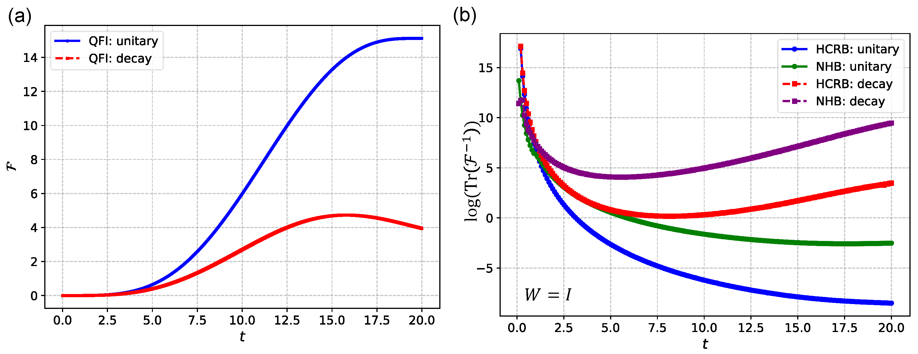
In Figure 2, we investigate the impact of noise on parameter estimation in many-body quantum systems without control. For single-parameter estimation, as clearly shown in Figure 2a, the QFI in the presence of environmental noise is significantly lower than that in the noiseless case. As for multiparameter estimation, as shown in Figure 2b, we explore the precision limits of multiparameter estimation without control. These limits are evaluated by the HCRB and NHB [53]. As shown in Figure 2, we can see that the environmental noise affects the precision of the parameter estimation. However, for multiparameters, precision of parameter estimation is not only affected by the environment, but also by the incompatibility between parameters.

In this work, we use quantum optimal control to mitigate the effect of noise on estimation accuracy and to alleviate the incompatibility problem in multiparameter estimation. Below, we introduce the quantum optimal control techniques used in our study, including the GRAPE, PSO, and DE.

3. Control-Enhanced Hamiltonian Optimization

In this work, we examine a controlled quantum system that is governed by a time-dependent Hamiltonian expressed as follows:

$$H\left(t\right)=H_0\left(\overrightarrow{x}\right)+\sum _{k=1}^p{V}_k\left(t\right)H_k,$$

(11)

Here, $H_0\left(\overrightarrow{x}\right)$ denotes the parameterized free evolution Hamiltonian where $\overrightarrow{x}$ represents the unknown parameter to be estimated. The term ${\sum }_{k=1}^p{V}_k\left(t\right)H_k$ characterizes the time-modulated control fields. In this context, the Hermitian operators $H_k$ ($k=1,2,\dots ,p$) encode the control channels, $V_k\left(t\right)$ stand for the tunable amplitudes of the corresponding external control fields, and t indicates time. The primary goal of optimal quantum control is to enhance the QFI $\mathcal{F}$ and QCRB $\mathrm{Tr}\left({\mathcal{F}}^{-1}\right)$. The quantum Fisher information quantifies the ultimate precision limit for estimating x and $\overrightarrow{x}$ by strategically designing the total Hamiltonian $H\left(t\right)=H_{\mathrm{LMG}}+H_{\mathrm{ctrl}}\left(t\right)$.

Within this framework, $H_{\mathrm{LMG}}$ represents the LMG Hamiltonian governing intrinsic spin interactions, while $H_{\mathrm{ctrl}}\left(t\right)={\sum }_k{V}_k\left(t\right)H_k$ denotes the adaptable control term. Through optimization of the temporal profiles $\left\{V_k\left(t\right)\right\}$, the objective is to mitigate decoherence effects, improve parameter sensitivity, and attain superior quantum-enhanced metrological performance beyond the limitations of uncontrolled system dynamics. This study focuses on optimizing the control Hamiltonian $H_{\mathrm{ctrl}}\left(t\right)$ using the QuanEstimation package [53], which incorporates three sophisticated algorithms: auto-GRAPE, PSO, and DE. These algorithms aim to enhance $\mathcal{F}$ by customizing $H_{\mathrm{ctrl}}\left(t\right)$ to counteract decoherence and enhance parameter sensitivity in the LMG system. The optimization objective is to minimize the weighted inverse of the QFIM for multiparameter estimation, defined as $\mathrm{Tr}\left(W·{\mathcal{F}}^{-1}\right)$, where W denotes the weighting matrix. For single parameter estimation, the aim is to maximize the QFI $\mathcal{F}$.

3.1. Control Optimization via Auto-GRAPE Algorithm

In the GRAPE algorithm [8], the control field is partitioned into M time slices, each lasting $\Delta t$. The control parameters $\left\{V_k^{\left(m\right)}\right\}$ indicate the strength of the k-th control field at the m-th slice and are updated iteratively through gradient ascent.

$$V_k^{\left(m\right)}\to V_k^{\left(m\right)}+\eta {\displaystyle \frac{\mathsf{\partial }\mathcal{F}}{\mathsf{\partial }{V}_k^{\left(m\right)}}},$$

(12)

Here, $\eta$ represents the learning rate and $\mathcal{F}$ stands for the QFI. An auto-GRAPE optimal control protocol is employed to maximize the QFI $\mathcal{F}$ for parameter estimation within experimentally constrained control resources. The control Hamiltonian $H_{\mathrm{ctrl}}\left(t\right)$ is parameterized by dividing the time domain $t\in [0,T]$ into M equally spaced intervals of length $\Delta t=T/M$, whereby the amplitude of each control field remains constant within each interval. This results in a piecewise constant control sequence $\left\{V_k^{\left(m\right)}\right\}$ ($k=x,y,z$; $m=1,2,\dots ,M$), where $V_k^{\left(m\right)}$ represents the strength of the k-th control channel during the m-th time step. The total control Hamiltonian is given by:

$$H_{\mathrm{ctrl}}\left(t\right)=\sum _{k=x,y,z}\sum _{m=1}^M{V}_k^{\left(m\right)}{J}_k,$$

(13)

Here, $J_{\alpha }={\displaystyle \frac{1}{2}}{\sum }_{i=1}^N{\sigma }_i^{\alpha }$ ($\alpha =x,y,z$) denote the collective spin operators. The gradient $\mathsf{\partial }\mathcal{F}/\mathsf{\partial }{V}_k^{\left(m\right)}$ is computed by applying the chain rule to the quantum master equation, considering the sensitivity of the density matrix $\rho \left(t\right)$ to variations in $V_k^{\left(m\right)}$. To ensure practical implementation, the control fields are confined to collective spin interactions $J_x,J_y,J_z$, achievable through global magnetic fields or laser-induced transitions in spin ensembles. Numerical simulations confirm that optimized pulse sequences $\left\{V_k^{\left(m\right)}\right\}$ enhance $\mathcal{F}$ by mitigating decoherence-related information loss and amplifying parameter-dependent coherence within the LMG system.

The proposed auto-GRAPE framework combines adaptive gradient ascent pulse engineering with quantum metrology dynamics, enabling automated enhancement of parameter estimation through optimization of control fields [53].

AD is a novel computational method utilized in machine learning to accurately compute derivatives of objective functions. By breaking down the objective function calculation into basic operations and employing the chain rule, AD not only delivers precise derivative outcomes but also maintains computational efficiency comparable to that of the objective function itself. Consequently, the ability to evaluate the gradient of the objective function holds significant importance.

This algorithm, a gradient-based optimization technique for quantum control problems, commences by initializing control amplitudes $V_k\left(t\right)$ for all time steps t and control parameters k, where k represents the control parameter index. Throughout each episode from 1 to M, the algorithm is provided with an initial quantum state ${\rho }_0$.

For each time step t ranging from 1 to T, the quantum state progresses based on the control equation:

$${\rho }_t=e^{\Delta t{\mathcal{L}}_t}{\rho }_{t-1},$$

(14)

Here, $\Delta t$ represents the size of the time step, ${\mathcal{L}}_t$ is the Liouvillian superoperator governing the quantum system’s dynamics at time t, ${\rho }_t$ signifies the quantum state at time step t. The derivatives of the quantum state concerning the parameters $\overrightarrow{x}$ are determined as:

$${\mathsf{\partial }}_{\overrightarrow{x}}{\rho }_t=-i\Delta t{\left[{\mathsf{\partial }}_{\overrightarrow{x}}{H}_{\mathrm{LMG}}\left(\overrightarrow{x}\right)\right]}^{\times }{\rho }_t+e^{\Delta t{\mathcal{L}}_t}{\mathsf{\partial }}_{\overrightarrow{x}}{\rho }_{t-1}.$$

(15)

Here, $\overrightarrow{x}$ represents the parameter vector, and $H_{\mathrm{LMG}}\left(\overrightarrow{x}\right)$ denotes the system Hamiltonian depending on parameters $\overrightarrow{x}$. The symbol ${[·]}^{\times }$ indicates the action of a superoperator on a density matrix. Upon evolving the state over all time steps, the algorithm computes the SLD and the objective function $\mathcal{F}$. The gradient of the objective function concerning the control amplitudes is then calculated using AD: ${\displaystyle \frac{\delta \mathcal{F}}{\delta V_k\left(t\right)}}$ for all t and k. For each time step t and each control parameter k, the control amplitudes are adjusted based on the gradient information:

$$V_{k+1}\left(t\right)=V_k\left(t\right)+\eta {\displaystyle \frac{\delta \mathcal{F}}{\delta V_k\left(t\right)}},$$

(16)

where $\eta$ represents the learning rate. This iterative process continues for multiple episodes until convergence, with the final optimized controls $\left\{V_k\left(t\right)\right\}$ and the corresponding objective function value $\mathcal{F}$ being stored at the conclusion. This algorithm effectively merges quantum state evolution with AD to enhance control parameters, ensuring accurate and efficient navigation of the quantum control landscape.

3.2. Control Optimization via PSO Algorithm

This research presents a quantum control optimization framework that employs PSO to enhance the accuracy of parameter estimation in open quantum systems [53]. The optimization process commences by configuring the control parameters ${\left\{V_k\right\}}_1^i$ for each particle i within the swarm $[1,P]$. Moreover, the velocity is set to ${\left\{\delta V_k\right\}}_1^i=0$ for each particle i in the swarm $[1,P]$. Each particle i in the swarm $[1,P]$ is given an initial personal best objective function value of $f\left({\left\{V_k\right\}}_{0,pb}^i\right)=0$. The objective function value f corresponds to either QFI ($\mathcal{F}$) or QCRB ($\mathrm{Tr}\left(W{\mathcal{F}}^{-1}\right)$).

For every iteration m ranging from 1 to M, and for each particle i from 1 to P, the algorithm obtains the current control ${\left\{V_k\right\}}_m^i$. Subsequently, it advances the quantum state using the current control ${\left\{V_k\right\}}_m^i$ and computes the objective function $f({\left\{V_k\right\}}_m^i)$ at the specified time T. Following this, it contrasts the current value of the objective function $f({\left\{V_k\right\}}_m^i)$ with the best personal value from the previous episode $f({\left\{V_k\right\}}_{m-1,pb}^i)$. The updated personal best is determined as:

$${\left\{V_k\right\}}_{m,pb}^i=arg\left(max\left\{f\left({\left\{V_k\right\}}_{m-1,pb}^i\right),f\left({\left\{V_k\right\}}_m^i\right)\right\}\right).$$

(17)

Once all personal bests have been updated for all particles, the algorithm compares all personal bests $f\left({\left\{V_k\right\}}_{m,pb}^i\right)$ for $i\in [1,P]$ and designates the global best as:

$${\left\{V_k\right\}}_{m,gb}=arg\left(\underset{i\in [1,P]}{max}f\left({\left\{V_k\right\}}_{m,pb}^i\right)\right),$$

(18)

where ${\left\{V_k\right\}}_{m,pb}^i$ stands for the personal best control parameters for the i-th particle at iteration m, and ${\left\{V_k\right\}}_{m,gb}$ represents the global best control parameters at iteration m. For each particle i from 1 to P, the velocity is adjusted using:

$${\left\{\delta V_k\right\}}_m^i=c_0{\left\{\delta V_k\right\}}_{m-1}^i+\mathrm{rand}\left(\right)·c_1({\left\{V_k\right\}}_{m,pb}^i-{\left\{V_k\right\}}_m^i)+\mathrm{rand}\left(\right)·c_2({\left\{V_k\right\}}_{m,gb}-{\left\{V_k\right\}}_m^i),$$

(19)

where the inertia weight coefficient is denoted by $c_0$, the cognitive (personal best) coefficient by $c_1$, and the social (global best) coefficient by $c_2$. The function $\mathrm{rand}(0,1)$ generates a random number between 0 and 1. Subsequently, the control parameters are updated as:

$${\left\{V_k\right\}}_{m+1}^i={\left\{V_k\right\}}_m^i+{\left\{\delta V_k\right\}}_m^i.$$

(20)

Upon completion of all iterations, the optimal global control ${\left\{V_k\right\}}_{M,gb}$ and the corresponding value of the objective function f are stored.

The algorithm updates the velocity and position of each particle iteratively based on its personal best experience and the global best experience of the entire swarm. The inertia weight $c_0$ helps balance exploration and exploitation, while the cognitive coefficient $c_1$ and social coefficient $c_2$ determine the impact of personal and global bests on the velocity update. The introduction of random numbers adds stochasticity, aiding the algorithm to avoid local optima. The state evolution step includes propagating the quantum state using the current control parameters and assessing the objective function at the target time T. This method effectively explores the control parameter space, aiming to discover optimal controls that enhance the desired quantum metric, and proves especially beneficial for intricate quantum control landscapes where gradient-based methods may face challenges.

3.3. Control Optimization via DE Algorithm

The approach utilizes a DE algorithm for optimizing quantum control problems [53]. Initially, it initializes the control parameters ${\left\{V_k\right\}}^i$ for each particle i in the swarm ($i\in [1,P]$). Subsequently, it propagates the quantum state under the current control ${\left\{V_k\right\}}^i$ and evaluates the objective function $f\left({\left\{V_k\right\}}^i\right)$ at time T for all $i\in [1,P]$. The objective function f represents either the QFI ($\mathcal{F}$) or the QCRB, $\mathrm{Tr}\left(W{\mathcal{F}}^{-1}\right)$.

For each generation from 1 to M, and for each particle $i\in [1,P]$, the algorithm:

1. Randomly selects three distinct indices $p_1,p_2,p_3$ from $[1,P]$, all different from i.

2. Generates the trial vector $\left\{G_k\right\}$ through mutation:

$$\left\{G_k\right\}={\left\{V_k\right\}}^{p_1}+c\left({\left\{V_k\right\}}^{p_2}-{\left\{V_k\right\}}^{p_3}\right),$$

(21)

where c is the mutation scaling factor controlling the differential weight.

3. Performs crossover between ${\left\{V_k\right\}}^i$ and $\left\{G_k\right\}$ to generate offspring controls.

• The intermediate vector $\left\{G_k\right\}$ is then used to update the swarm for the next generation.

For each $k\in [1,K]$, the algorithm generates a random integer $a\in [1,N_c]$, where $N_c$ denotes the total number of control parameters. For each $j\in [1,N_c]$, it generates a random number $r\in [0,1]$ and assigns:

$${\left[Q_k\right]}_j=\left\{\begin{array}{cc}{\left[G_k\right]}_j,\hfill & \mathrm{if}r\le c_r\mathrm{or}j=a,\hfill \\ {[V_k]}_j,\hfill & \mathrm{if}r>c_r\mathrm{and}j\ne a,\hfill \end{array}\right.$$

(22)

where $c_r$ is the crossover probability determining the likelihood of parameter transfer from the mutant vector, and $\left\{Q_k\right\}$ is the trial control generated after crossover.

After generating $\left\{Q_k\right\}$, the algorithm propagates the quantum state under the new control and evaluates $f\left(\left\{Q_k\right\}\right)$ at time T. If $f\left(\left\{Q_k\right\}\right)>f\left({\left\{V_k\right\}}^i\right)$, the particle updates its control to $\left\{Q_k\right\}$. After completing all generations, the algorithm identifies the global best control ${\left\{V_k\right\}}^{*}$ by selecting the particle with the maximum objective value f.

This DE-based algorithm optimizes control parameters in quantum systems. It maintains a population of candidate control sets and iteratively refines the solutions through mutation, crossover, and selection.

(1) Mutation introduces diversity via differential perturbations between existing solutions.

(2) Crossover mixes parameters from the original and mutant vectors to generate a trial vector.

(3) Selection retains superior solutions for the next generation based on fitness comparisons.

The algorithm efficiently explores the parameter space to identify controls that maximize the target quantum metric (e.g., Quantum Fisher Information or QCRB). Its stochastic nature enables robust exploration of complex control landscapes, avoiding local optima that often trap gradient-based methods.

Our theoretical framework has direct relevance to several cutting-edge experimental platforms in quantum metrology. Recent advances in trapped-ion systems [58,59], superconducting quantum circuits [60,61], and ultracold atomic ensembles [62] have demonstrated precise Hamiltonian engineering and control capabilities that could readily implement the optimized protocols presented in this work. For instance, the auto-GRAPE algorithm’s control sequences could be directly applied to trapped-ion quantum simulators where time-dependent magnetic field gradients and laser intensities can be precisely modulated to realize the optimized control Hamiltonians.

4. Algorithm Comparison

The auto-GRAPE algorithm leverages analytical gradients of the QFIM with respect to control parameters, enabling efficient navigation of the optimization landscape. Its theoretical advantage stems from the exploitation of first-order derivative information, guaranteeing rapid convergence to local optima for smooth objective functions. The integration of the Adam optimizer further enhances its performance through adaptive learning rates and momentum-based acceleration.

DE, in contrast, employs a population-based approach that operates without gradient information. This evolutionary algorithm explores the parameter space through mutation, crossover, and selection operations, providing robust global optimization capabilities particularly valuable for non-convex landscapes. Its independence from gradient calculations makes it especially suitable for complex quantum systems where analytical derivatives may be challenging to obtain or computationally expensive.

PSO utilizes collective intelligence principles, where candidate solutions (“particles”) navigate the search space by balancing individual best-known positions with global best-known positions. This algorithm theoretically offers an optimal balance between exploration (global search) and exploitation (local refinement), though its performance is sensitive to parameter tuning including inertia weights and cognitive/social coefficients.

We evaluate these algorithms on two paradigmatic many-body quantum systems: the two-spin Ising model and the collective spin system described by the LMG Hamiltonian. The optimization objective in both cases is the minimization of the QCRB, $\mathrm{Tr}({\mathcal{F}}^{(}-1))$, which quantifies the QCRB for multiparameter estimation.

4.1. Single Parameter Estimation

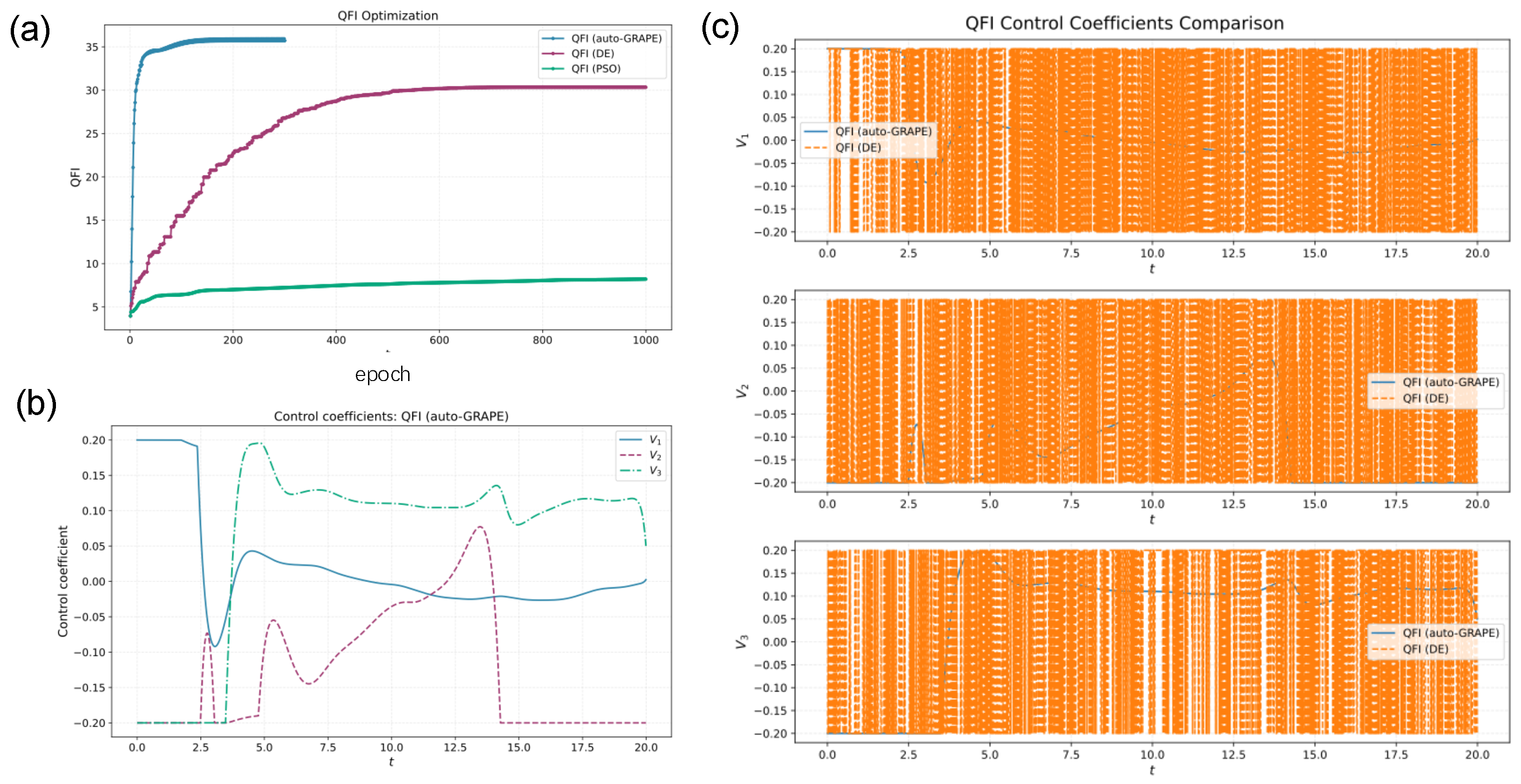
The performance of three distinct optimization algorithms for single-parameter estimation is comprehensively evaluated in our numerical simulations. Figure 3a presents the QFI evolution with respect to training epochs for auto-GRAPE, DE, and PSO. The quantitative results are summarized in

Table 1. Performance comparison of optimization algorithms for single-parameter estimation. The QFI values, enhancement factors, relative improvements, convergence iterations, and key parameters are summarized under identical system conditions ($N=2$, $\gamma =2\pi /100$). Control amplitudes were constrained to $[-0.2,0.2]$.

Algorithm	Uncontrolled QFI	Optimized QFI	Relative Improvement (%)	Iterations to Convergence
auto-GRAPE	3.954	35.72	9.04	299
DE	3.954	30.350	7.68	999
PSO	3.954	8.21	2.08	1999

, revealing substantial differences in algorithmic efficiency and enhancement capability.

Auto-GRAPE demonstrates exceptional performance with rapid convergence, achieving $\mathcal{F}\approx 35.72$ within merely 299 epochs and maintaining stability thereafter. This represents a 9.04-fold enhancement over the uncontrolled system ($\mathcal{F}\approx 3.95$). DE exhibits strong performance with $\mathcal{F}\approx 30.35$ ($7.68$-fold enhancement) but requires the full 999 iterations to converge. PSO shows the slowest convergence rate and lowest final QFI value ($\mathcal{F}\approx 8.21$), yielding only marginal improvement over the uncontrolled case.

To gain deeper insights into the dynamic behavior of the auto-GRAPE algorithm during the optimization process, we analyzed the evolution of its control coefficients over iterations. As shown in Figure 3b, throughout the optimization process, the control coefficients of the auto-GRAPE algorithm exhibit significant variations, reflecting the adaptive adjustments made by the algorithm to achieve the optimal solution. Initially, there are rapid fluctuations in the control coefficients, which gradually stabilize. This indicates that the algorithm has identified a region close to the optimal solution and begins fine-tuning to further enhance performance metrics.

To further validate the advantages of the auto-GRAPE algorithm over other optimization algorithms, we compared the evolution of its control coefficients with those of the Differential Evolution (DE) algorithm, as illustrated in Figure 3c. The results clearly demonstrate that the auto-GRAPE algorithm exhibits superior convergence speed and final stability. Specifically, the auto-GRAPE algorithm not only reaches stable control coefficient values more quickly but also maintains lower variability throughout the optimization process. This highlights the high efficiency and reliability of the auto-GRAPE algorithm in handling complex optimization problems.

Table 1, performance comparison of optimization algorithms for single-parameter estimation. These findings establish auto-GRAPE as the optimal choice for single-parameter quantum estimation tasks when analytical gradients are accessible, offering superior performance with significantly reduced computational overhead. For experimental implementations where gradient calculation may be challenging, DE provides a viable alternative with robust global optimization capabilities, albeit at the cost of increased computational resources.

The superior performance of auto-GRAPE stems from its gradient-based optimization framework that efficiently navigates the control landscape through analytical derivatives of the QFI with respect to control parameters. Its integration with the Adam optimizer further enhances convergence through adaptive learning rates and momentum-based acceleration. DE’s evolutionary approach provides robust global optimization capabilities without requiring gradient information, making it particularly valuable for complex quantum systems where analytical derivatives may be challenging to obtain. PSO’s suboptimal performance in this context likely results from its search strategy being less compatible with the specific topological features of the quantum control landscape for parameter estimation.

4.2. MultiParameter Estimation

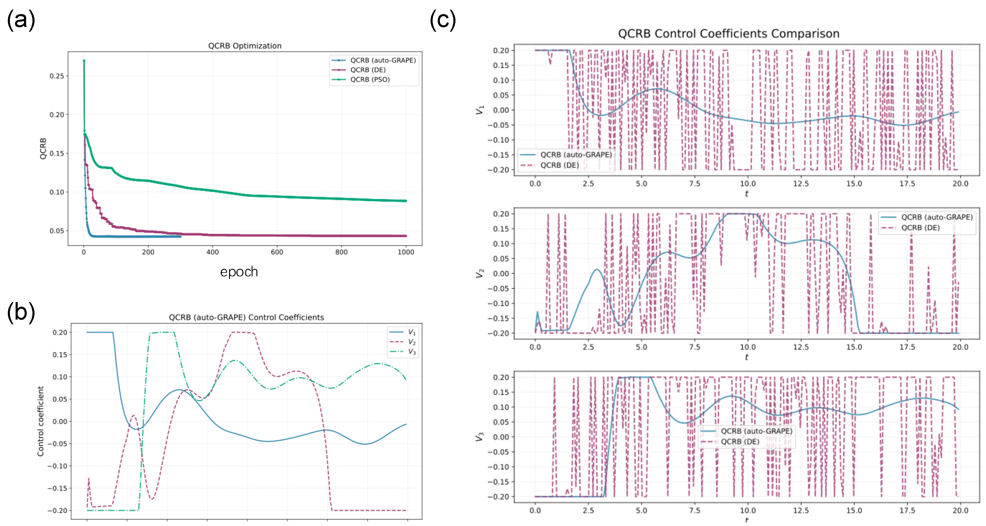
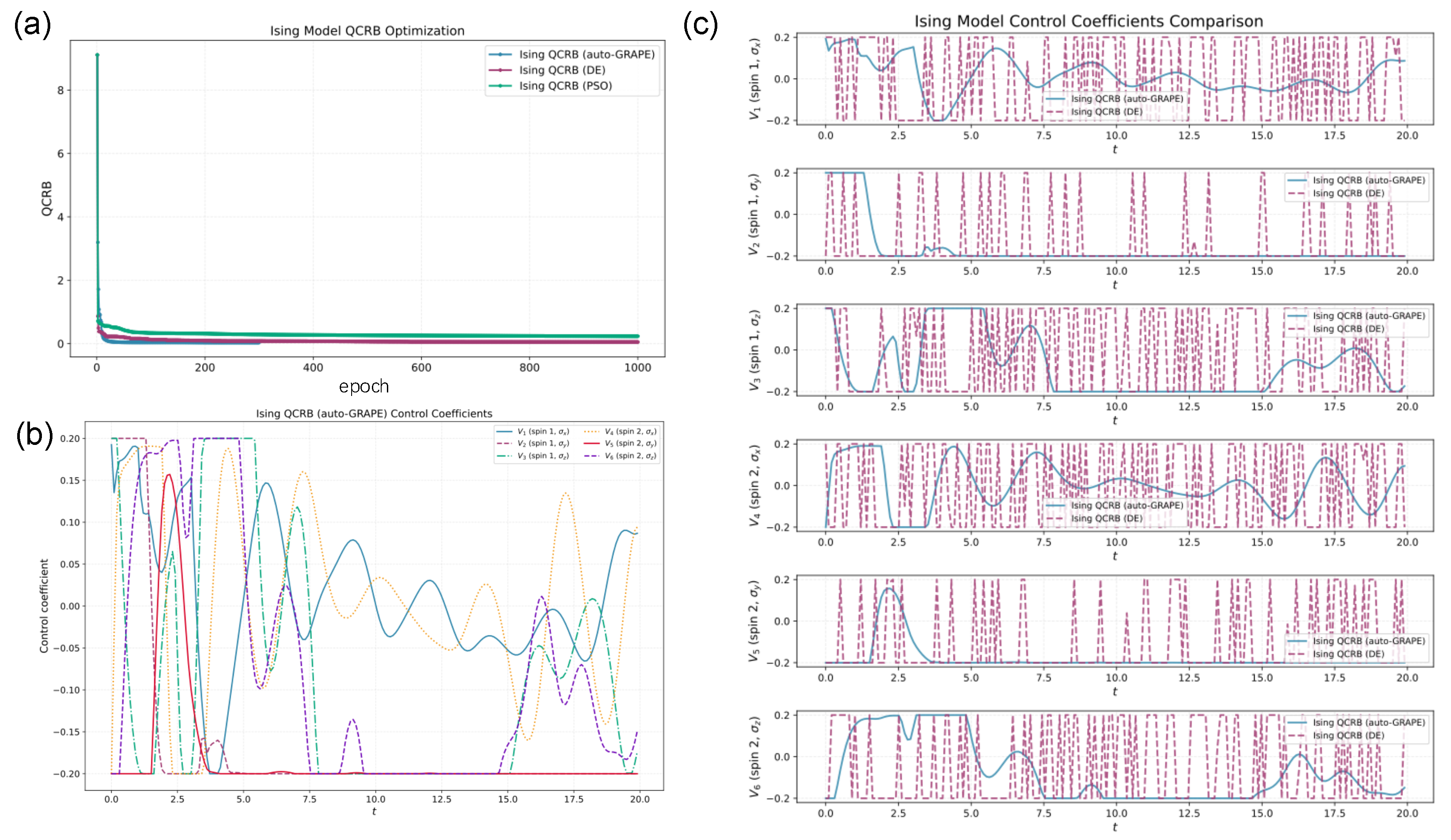
In multiparameter estimation for the simultaneous determination, the QFIM ${\mathcal{F}}_{ij}$ unveils trade-offs in precision. Control optimization diminishes the condition number of ${\mathcal{F}}_{ij}$, thus reducing the incompatibility between parameters. In the pursuit of enhanced quantum parameter estimation, we investigate three distinct optimization algorithms for engineering time-dependent control Hamiltonians: the gradient-based auto-GRAPE algorithm, the evolutionary DE algorithm, and the PSO algorithm, as shown in Figure 4 and Figure 5, which assesses the precision limits in multiparameter quantum metrology through the QCRB, quantified by the trace of the inverse QFIM, $\mathrm{Tr}\left({\mathcal{F}}^{-1}\right)$.

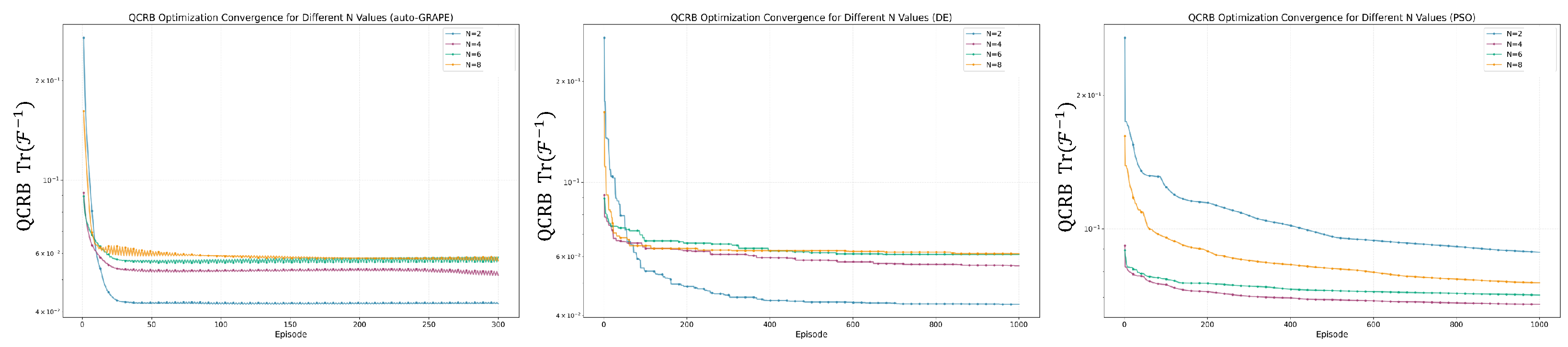
For the collective spin system governed by the LMG Hamiltonian $H_0=-\lambda (J_x^2+g{J}_y^2)/N-h{J}_z$ with $\lambda =1.0,g=0.5$, and $h=0.1$, in Figure 4 the uncontrolled system exhibits a QCRB of 0.269757. Under identical dephasing conditions, the optimization outcomes are: auto-GRAPE: Reaches a QCRB of 0.042288 after 299 iterations, representing a 6.37-fold improvement. The convergence behavior demonstrates the algorithm’s efficiency even in systems with limited optimization potential. DE: Achieves a QCRB of 0.043242 after 999 iterations, a 6.23-fold enhancement. Remarkably, DE’s performance is within 2.2% of auto-GRAPE’s result, demonstrating exceptional efficacy for this particular model despite its gradient-free nature. PSO: Converges to a QCRB of 0.088451 after 1000 iterations, providing only a $3.05$-fold improvement. The significant performance gap (higher than auto-GRAPE) suggests algorithmic incompatibility with the LMG model’s optimization landscape. Further, we show the impact of different Nunder the three algorithms in Figure 6, and it can be seen that the GRAPE algorithm shows better optimization efficiency.

For the two-spin Ising model with Hamiltonian $H_0=J({\sigma }_x\otimes {\sigma }_x)-h({\sigma }_z\otimes I+I\otimes {\sigma }_z)$, in Figure 5, where $J=1.0$ and $h=0.1$ represent the coupling strength and transverse field respectively, the uncontrolled system exhibits a QCRB of 9.111005. Under dissipative dynamics with dephasing rate $\gamma =2\pi /100$, the optimization algorithms achieve the following results: auto-GRAPE: Achieves a QCRB of 0.034635 after 299 iterations, representing a $263.2$-fold improvement over the uncontrolled case. The algorithm demonstrates rapid convergence within the first 100 iterations, with diminishing returns thereafter. DE: Converges to a QCRB of 0.052817 after 999 iterations, providing a $172.5$-fold enhancement. PSO: Yields a QCRB of 0.233315 after 1000 iterations, a $39.1$-fold improvement.

This

Table 2. Performance comparison of optimization algorithms on Ising and LMG models. The QCRB, with lower values indicating superior parameter estimation precision. Improvement ratio is calculated relative to the uncontrolled system (Ising: 9.111005, LMG: 0.269757).

Model & Metric	Uncontrolled	Auto-GRAPE	DE	PSO
Ising Model
QCRB	9.111005	0.034635	0.052817	0.233315
Improvement ratio	1×	263.2×	172.5×	39.1×
Iterations to convergence	-	299	999	1000
LMG Model
QCRB	0.269757	0.042288	0.043242	0.088451
Improvement ratio	1×	6.37×	6.23×	3.05×
Iterations to convergence	-	299	999	1000

quantitatively demonstrates the superior performance of gradient-based optimization (auto-GRAPE) for quantum parameter estimation tasks in many-body systems when analytical gradients are available. The exceptional performance of DE on the LMG model highlights its value as a gradient-free alternative for complex quantum systems where derivative calculations may be impractical. The significant performance gap observed with PSO suggests algorithm-specific incompatibility with the quantum control landscapes of these particular many-body models. These findings provide crucial guidance for selecting appropriate optimization strategies based on system characteristics, available computational resources, and gradient accessibility in experimental quantum metrology implementations.

These results collectively demonstrate that Hamiltonian optimization control significantly enhances parameter estimation precision in many-body quantum systems while simultaneously suppressing noise-induced errors. The gradient-driven auto-GRAPE algorithm achieves the lowest QCRB across systems, aligning with theoretical expectations for multiparameter estimation in open quantum systems. However, the strong performance of DE in the LMG model highlights the importance of algorithm selection based on specific physical system characteristics and available computational resources.

5. Conclusions

In this work, we explore the theory of optimizing Hamiltonian control in many-body quantum systems to enhance the precision of quantum parameter estimation. This approach addresses key challenges in achieving quantum-enhanced parameter estimation in many-body systems. We explore the LMG model, Ising model, the paradigmatic system with spin interactions, as a testbed for optimizing time-dependent control fields through the GRAPE, PSO, and DE algorithms. Our numerical experiments show that Hamiltonian optimization control significantly improves the precision of parameter estimation, suppresses noise-induced errors, and alleviates incompatibility issues in multiparameter estimation. The gradient-based auto-GRAPE algorithm, in particular, achieves the best performance. These findings advance the practical implementation of quantum-enhanced metrology and offer a path toward Heisenberg-limited sensing in noisy environments.

References

1. Liu, J.; Yuan, H.D.; Lu, X.-M.; Wang, X.G. Quantum Fisher information matrix and multiparameter estimation. J. Phys. A Math. Theor. 2020, 53, 023001. [Google Scholar] [CrossRef]
2. Braunstein, S.L. Quantum limits on precision measurements of phase. Phys. Rev. Lett. 1992, 69, 3598–3601. [Google Scholar] [CrossRef]
3. Vittorio, G.; Seth, L.; Lorenzo, M. Quantum-Enhanced Measurements: Beating the Standard Quantum Limit. Science 2004, 306, 1330–1336. [Google Scholar] [CrossRef]
4. Tao, H.; Su, Y.G.; Zhang, X.Y.; Liu, J.; Wang, X.G. Lee-Yang zeros and quantum Fisher information matrix in a nonlinear system. Phys. Rev. E 2023, 108, 024104. [Google Scholar] [CrossRef]
5. Tao, H.; Shao, L.; Zhang, Z.C.; Zhang, X.Y.; Zhang, R.; Chen, J.; Lu, W.J. Quantum Fisher Information and Lee-Yang Zeros with Quantum Coherence of the Isotropic XY Model and the Energy Scale. Ann. Phys 2022, 534, 2200291. [Google Scholar] [CrossRef]
6. Joo, J.; Munro, W.J.; Spiller, T.P. Quantum Metrology with Entangled Coherent States. Phys. Rev. Lett. 2011, 107, 083601. [Google Scholar] [CrossRef]
7. Qin, J.-F.; Xu, Y.; Liu, J. Optimal finite-dimensional probe states for quantum phase estimation. Phys. Rev. A 2006, 112, 052428. [Google Scholar] [CrossRef]
8. Liu, J.; Yuan, H. Quantum parameter estimation with optimal control. Phys. Rev. A 2017, 96, 012117. [Google Scholar] [CrossRef]
9. Liu, J.; Yuan, H.D. Control-enhanced multiparameter quantum estimation. Phys. Rev. A 2017, 96, 042114. [Google Scholar] [CrossRef]
10. Yuan, H.D.; Fung, C.F. Optimal Feedback Scheme and Universal Time Scaling for Hamiltonian Parameter Estimation. Phys. Rev. Lett. 2015, 15, 110401. [Google Scholar] [CrossRef]
11. Baumgratz, T.; d Datta, A. Quantum Enhanced Estimation of a Multidimensional Field. Phys. Rev. Lett. 2016, 116, 030801. [Google Scholar] [CrossRef]
12. Liu, J.; Jing, X.X.; Wang, X.G. Phase-matching condition for enhancement of phase sensitivity in quantum metrology. Phys. Rev. A 2013, 88, 042316. [Google Scholar] [CrossRef]
13. Braun, D.; Adesso, G.; Benatti, F.; Floreanini, R.; Marzolino, U.; Mitchell, M.W.; Pirandola, S. Quantum-enhanced measurements without entanglement. Rev. Mod. Phys. 2018, 90, 035006. [Google Scholar] [CrossRef]
14. Ilias, T.; Yang, D.; Huelga, S.F.; Plenio, M.B. Criticality-Enhanced Quantum Sensing via Continuous Measurement. PRX Quantum 2022, 3, 010354. [Google Scholar] [CrossRef]
15. Linnemann, D.; Strobel, H.; Muessel, W.; Schulz, J.; Lewis-Swan, R.J.; Kheruntsyan, K.V.; Oberthaler, M.K. Quantum-Enhanced Sensing Based on Time Reversal of Nonlinear Dynamics. Phys. Rev. Lett. 2016, 117, 013001. [Google Scholar] [CrossRef]
16. Pál, K.F.; Tóth, G.; Bene, E.; Vértesi, T. Bound entangled singlet-like states for quantum metrology. Phys. Rev. Res. 2021, 3, 023101. [Google Scholar] [CrossRef]
17. Liu, J.; Lu, X.M.; Sun, Z.; Wang, X.G. Quantum multiparameter metrology with generalized entangled coherent state. J. Phys. A Math. Theor. 2016, 49, 115302. [Google Scholar] [CrossRef]
18. Helstrom, C.W. Quantum Detection and Estimation Theory; Academic: New York, NY, USA, 1976. [Google Scholar]
19. Holevo, A.S. Probabilistic and Statistical Aspects of Quantum Theory; North-Holland: Amsterdam, The Netherlands, 1982. [Google Scholar]
20. Ito, S.; Dechant, A. Stochastic Time Evolution, Information Geometry, and the Cram’er-Rao Bound. Phys. Rev. X 2020, 10, 021056. [Google Scholar] [CrossRef]
21. Braunstein, S.L.; Caves, C.M.; Milburn, G.J. Generalized Uncertainty Relations: Theory, Examples, and Lorentz Invariance. Ann. Phys. 1996, 247, 135–173. [Google Scholar] [CrossRef]
22. Giovannetti, V.; Lloyd, S.; Maccone, L. Quantum Metrology. Phys. Rev. Lett. 2006, 96, 010401. [Google Scholar] [CrossRef]
23. Alipour, S.; Mehboudi, M.; Rezakhani, A.T. Quantum Metrology in Open Systems: Dissipative Cram’er-Rao Bound. Phys. Rev. Lett. 2014, 112, 120405. [Google Scholar] [CrossRef]
24. Braunstein, S.L.; Caves, C.M. Statistical Distance and the Geometry of Quantum States. Phys. Rev. Lett. 1994, 72, 3439–3443. [Google Scholar] [CrossRef]
25. Zwierz, M.; Pérez-Delgado, C.A.; Kok, P. General Optimality of the Heisenberg Limit for Quantum Metrology. Phys. Rev. Lett. 2010, 105, 180402. [Google Scholar] [CrossRef]
26. Sidhu, J.S.; Kok, P. Geometric Perspective on Quantum Parameter Estimation. AVS Quantum Sci. 2020, 2, 014701. [Google Scholar] [CrossRef]
27. Wang, W.; Wu, Y.; Ma, Y.; Cai, W.; Hu, L.; Mu, X.; Xu, Y.; Chen, Z.-J.; Wang, H.; Song, Y.P.; et al. Heisenberg-Limited Single-Mode Quantum Metrology in a Superconducting Circuit. Nature Commun. 2019, 10, 4382. [Google Scholar] [CrossRef]
28. Tao, H.; Huang, R.; Tan, X.Q. Quantum Parameter Estimation With Graph States In SU(N) Dynamics. Adv. Quantum Technol. 2024, 7, 2300254. [Google Scholar] [CrossRef]
29. Liu, J.; Jing, X.-X.; Zhong, W.; Wang, X.G. Quantum Fisher Information for Density Matrices with Arbitrary Ranks. Commun. Theor. Phys. 2014, 61, 45. [Google Scholar] [CrossRef]
30. Lipkin, H.J.; Meshkov, N.; Glick, A.J. Validity of Many-Body Approximation Methods for a Solvable Model: (I). Exact Solutions and Perturbation Theory. Nuclear Phys. 1965, 62, 188–198. [Google Scholar] [CrossRef]
31. Choi, J.; Zhou, H.; Knowles, H.S.; Landig, R.; Choi, S.; Lukin, M.D. Robust Dynamic Hamiltonian Engineering of Many-Body Spin Systems. Phys. Rev. X 2020, 10, 031002. [Google Scholar] [CrossRef]
32. Beau, M.; del Campo, A. Nonlinear Quantum Metrology of Many-Body Open Systems. Phys. Rev. Lett. 2017, 119, 010403. [Google Scholar] [CrossRef]
33. Niezgoda, A.; Chwede’nczuk, J. Many-Body Nonlocality as a Resource for Quantum-Enhanced Metrology. Phys. Rev. Lett. 2021, 126, 210506. [Google Scholar] [CrossRef]
34. Cui, H.T. Multiparticle Entanglement in the Lipkin-Meshkov-Glick Model. Phys. Rev. A 2008, 77, 052105. [Google Scholar] [CrossRef]
35. Solinas, P.; Ribeiro, P.; Mosseri, R. Dynamical Properties Across a Quantum Phase Transition in the Lipkin-Meshkov-Glick Model. Phys. Rev. A 2008, 78, 052329. [Google Scholar] [CrossRef]
36. Salvatori, G.; Mandarino, A.; Paris, M.G.A. Quantum Metrology in Lipkin-Meshkov-Glick Critical Systems. Phys. Rev. A 2014, 90, 022111. [Google Scholar] [CrossRef]
37. Xu, K.; Zhang, Y.-R.; Sun, Z.-H.; Li, H.; Song, P.; Xiang, Z.; Huang, K.; Li, H.; Shi, Y.-H.; Chen, C.-T.; et al. Metrological Characterization of Non-Gaussian Entangled States of Superconducting Qubits. Phys. Rev. Lett. 2022, 128, 150501. [Google Scholar] [CrossRef] [PubMed]
38. Pezzè, L.; Smerzi, A.; Oberthaler, M.K.; Schmied, R.; Treutlein, P. Quantum Metrology with Nonclassical States of Atomic Ensembles. Rev. Mod. Phys. 2018, 90, 035005. [Google Scholar] [CrossRef]
39. Hotter, C.; Ritsch, H.; Gietka, K. Combining Critical and Quantum Metrology. Phys. Rev. Lett. 2024, 132, 060801. [Google Scholar] [CrossRef]
40. Frérrot, I.; Roscilde, T. Quantum Critical Metrology. Phys. Rev. Lett. 2018, 121, 020402. [Google Scholar] [CrossRef]
41. Ding, D.-S.; Liu, Z.-K.; Shi, B.-S.; Guo, G.-C.; Mølmer, K.; Adams, C.S. Enhanced Metrology at the Critical Point of a Many-Body Rydberg Atomic System. Nat. Phys. 2022, 18, 1447–1452. [Google Scholar] [CrossRef]
42. Liu, R.; Chen, Y.; Jiang, M.; Yang, X.; Wu, Z.; Li, Y.; Yuan, H.; Peng, X.; Du, J. Experimental Critical Quantum Metrology with the Heisenberg Scaling. npj Quantum Inf. 2021, 7, 170. [Google Scholar] [CrossRef]
43. Mihailescu, G.; Bayat, A.; Campbell, S.; Mitchell, A.K. Multiparameter Critical Quantum Metrology with Impurity Probes. Quantum Sci. Technol. 2024, 9, 035033. [Google Scholar] [CrossRef]
44. Liu, J.; Zhang, M.; Chen, H.; Wang, L.; Yuan, H. Optimal Scheme for Quantum Metrology. Adv. Quantum Technol. 2022, 5, 2100080. [Google Scholar] [CrossRef]
45. Pang, S.; Jordan, A.N. Optimal Adaptive Control for Quantum Metrology with Time-Dependent Hamiltonians. Nat. Commun. 2017, 8, 14695. [Google Scholar] [CrossRef]
46. Xu, H.; Li, J.; Liu, L.; Wang, Y.; Yuan, H.; Wang, X. Generalizable Control for Quantum Parameter Estimation through Reinforcement Learning. npj Quantum Inf. 2019, 5, 82. [Google Scholar] [CrossRef]
47. Zhou, S. Limits of Noisy Quantum Metrology with Restricted Quantum Controls. Phys. Rev. Lett. 2024, 133, 170801. [Google Scholar] [CrossRef]
48. Yang, J.; Pang, S.; Chen, Z.; Jordan, A.N.; del Campo, A. Variational Principle for Optimal Quantum Controls in Quantum Metrology. Phys. Rev. Lett. 2022, 128, 160505. [Google Scholar] [CrossRef]
49. Li, Z.; Colombo, S.; Shu, C.; Velez, G.; Pilatowsky-Cameo, S.; Schmied, R.; Choi, S.; Lukin, M.; Pedrozo-Peñafiel, E.; Vuletić, V. Improving Metrology with Quantum Scrambling. Science 2023, 380, 1381–1384. [Google Scholar] [CrossRef]
50. Yu, X.; Zhao, X.; Li, L.; Hu, X.-M.; Duan, X.; Yuan, H.; Zhang, C. Toward Heisenberg Scaling in Non-Hermitian Metrology at the Quantum Regime. Sci. Adv. 2024, 10, eadk7616. [Google Scholar] [CrossRef] [PubMed]
51. Lu, W.; Peng, Z.-H.; Tao, H. Information Geometry and Parameter Sensitivity of Non-Hermitian Hamiltonians. Phys. Lett. A 2024, 525, 129919. [Google Scholar] [CrossRef]
52. Li, J.; Liu, H.; Wang, Z.; Yi, X.X. Enhanced Parameter Estimation by Measurement of Non-Hermitian Operators. AAPPS Bull. 2023, 33, 22. [Google Scholar] [CrossRef]
53. Zhang, M.; Yu, H.-M.; Yuan, H.; Wang, X.; Demkowicz-Dobrza’nski, R.; Liu, J. QuanEstimation: An Open-Source Toolkit for Quantum Parameter Estimation. Phys. Rev. Res. 2022, 4, 043057. [Google Scholar] [CrossRef]
54. Khaneja, N.; Reiss, T.; Kehlet, C.; Schulte-Herbrüggen, T.; Glaser, S.J. Optimal Control of Coupled Spin Dynamics: Design of NMR Pulse Sequences by Gradient Ascent Algorithms. J. Magn. Reson. 2005, 172, 296–305. [Google Scholar] [CrossRef]
55. Yu H.-M, M.; Liu, J. Quanestimation.jl: An open-source Julia framework for quantum parameter estimation. Fundam. Res. 2025. [Google Scholar] [CrossRef]
56. Demkowicz-Dobrzański, R.; Górecki, W.; Guţă, M. multiparameter estimation beyond quantum Fisher information. J. Phys. A Math. Theor. 2020, 53, 363001. [Google Scholar] [CrossRef]
57. Conlon, L.O.; Suzuki, J.; Lam, P.K.; Assad, S.M. Efficient computation of the Nagaoka–Hayashi bound for multiparameter estimation with separable measurements. NPJ Quantum Inf. 2021, 7, 110. [Google Scholar] [CrossRef]
58. Huang, Y.X.; Wu, W.; Mei, Q.Y.; Lin, Y.H. Experimental proposal on scalable radio-frequency magnetometer with trapped ions. Phys. Rev. Appl. 2025, 24, L061002. [Google Scholar] [CrossRef]
59. Valahu, C.H.; Stafford, M.P.; Huang, Z.; Matsos, V.G.; Millican, M.J.; Chalermpusitarak, T.; Menicucci, N.C.; Combes, J.; Baragiola, B.Q.; Tan, T.R. Quantum-enhanced multiparameter sensing in a single mode. Sci. Adv. 2025, 11, eadw9757. [Google Scholar] [CrossRef] [PubMed]
60. Deng, X.; Li, S.; Chen, Z.-J.; Ni, Z.; Cai, Y.; Mai, J.; Zhang, L.; Zheng, P.; Yu, H.; Zou, C.-L.; et al. Quantum-enhanced metrology with large Fock states. Nat. Phys. 2024, 20, 1874–1880. [Google Scholar] [CrossRef]
61. Wang, W.; Chen, Z.-J.; Liu, X.; Cai, W.; Ma, Y.; Mu, X.; Pan, X.; Hua, Z.; Hu, L.; Xu, Y.; et al. Quantum-enhanced radiometry via approximate quantum error correction. Nat. Commun. 2022, 13, 3214. [Google Scholar] [CrossRef]
62. Mao, T.-W.; Liu, Q.; Li, X.-W.; Cao, J.-H.; Chen, F.; Xu, W.-X.; Tey, M.K.; Huang, Y.-X.; You, L. Quantum-enhanced sensing by echoing spin-nematic squeezing in atomic Bose–Einstein condensate. Nat. Phys. 2023, 19, 1585–1590. [Google Scholar] [CrossRef]
Figure 1. Quantum Parameter Estimation Optimization Control Scheme. (a) sequential scheme, (b) parallel scheme, (c) controlled parallel scheme.
Metrology 06 00017 g001
Figure 2. (a) The evolution of normalized QFI by time t. The blue line represents the value of the QFI for unitary evolution without controls. The red line represents the value of the QFI for noise decay with decay rate γ = π / 50 . The true value of g is assumed to be 1. (b) Log Plots of the QCRB evolution over time for multiparameter estimation for LMG model with no control. The blue dotted line indicates HCRB under the unitary evolution and the green dotted line indicates NHB under the unitary evolution, and W = I is identity matrix. Red and purple lines indicate HCRB and NHB under decaying conditions with decay rate γ = π / 5 , respectively.
Metrology 06 00017 g002
Figure 3. Illustration of the QFI for single-parameter estimation with LMG model. (a) the QFI is plotted with control algorithms (auto-GRAPE, PSO, DE). (b) the control fields are plotted over time t for auto-GRAPE algorithm. The control fields V 1 , V 2 , V 3 with the control field I x , J y , J z , respectively. (c) Comparison of the trends of the control field ( J x , J y , J Z ) of the (auto-GRAPE, DE) algorithms.
Metrology 06 00017 g003
Figure 4. Illustrating of the QCRB for multiparameter estimation with LMG model. (a) QCRB Tr ( F 1 ) is plotted with control algorithms (auto-GRAPE, PSO, and DE algorithms). (b) the control fields δ g are plotted over time t for auto-GRAPE algorithm. The control fields V 1 , V 2 , V 3 with the control field I x , J y , J z , respectively. (c) Compare the trend of the control field ( J x , J y , J Z ) of the (auto-GRAPE, DE) algorithm.
Metrology 06 00017 g004
Figure 5. Illustrating the QCRB for multiparameter estimation with Ising model. (a) QCRB Tr ( F 1 ) is plotted with control algorithms (auto-GRAPE algorithm, PSO algorithm, DE algorithm). (b) the control fields δ g are plotted over time t for auto-GRAPE algorithm. The control fields V 1 , V 2 , V 3 with the control field σ x 1 , σ y 1 , σ z 1 , σ x 2 , σ y 2 , σ z 2 , respectively. (c) Compare the trend of the control field ( σ x 1 , σ y 1 , σ z 1 , σ x 2 , σ y 2 , σ z 2 ) of the (auto-GRAPE, DE) algorithm.
Metrology 06 00017 g005
Figure 6. Illustrating the QCRB for multiparameter estimation with N-spin LMG model for different N. (ac) QCRB Tr ( F 1 ) is plotted with control algorithms auto-GRAPE algorithm, PSO algorithm, DE algorithm).
Metrology 06 00017 g006