Simulation Uncertainty for a Virtual Ultrasonic Flow Meter

Abstract

Ultrasonic clamp-on meters have become an established technology for non-invasive flow measurements. Under disturbed flow conditions, their measurement values must be adjusted with corresponding fluid mechanical calibration factors. Due to the variety of flow disturbances and installation positions, the experimental determination of these factors often needs to be complemented by computational fluid dynamics (CFD) simulations. From a metrological perspective, substituting experiments with simulation results raises the question of how confidence in a so-called virtual measurement can be ensured. While there are well-established methods to estimate errors in CFD predictions in general, strategies to meet metrological requirements for CFD-based virtual meters have yet to be developed. In this paper, a framework for assessing the overall uncertainty of a virtual flow meter is proposed. In analogy to the evaluation of measurement uncertainty, the approach is based on the utilization of an expanded simulation uncertainty representing the entirety of the computational domain. The study was conducted using the example of an ultrasonic clamp-on meter downstream of a double bend out-of-plane. Nevertheless, the proposed method applies to other flow disturbances and different types of virtual meters. The comparison between laboratory experiments and simulation results with different turbulence modeling approaches demonstrates a clear superiority of hybrid RANS-LES models over the industry standard RANS. With an expanded simulation uncertainty of 1.44 × 10⁻², the virtual measurement obtained with a hybrid model allows for a continuous determination of calibration factors applicable to the relevant mounting positions of a real meter at a satisfactory level of confidence.

1. Introduction

Ultrasonic clamp-on meters have become an established technology for non-invasive flow measurements in industrial applications. As a portable device, they can be used at multiple measurement positions without interrupting the ongoing processes and are suitable for a wide range of fluids, temperatures, and conduit sizes. On the downside, the comparatively simple measuring principle can result in large measurement deviations under non-ideal (disturbed) flow conditions caused by bend configurations, valves, reductions, pumps, and other components installed upstream. For this reason, the measurement value has to be adjusted by means of fluid mechanical calibration factors, hereinafter referred to as $K_d$. In that regard, $K_d$ acts as a constant of proportionality between the mean velocity in the pipe and the averaged velocity over the ultrasonic path as determined by the meter. Its magnitude can vary significantly (≈$\pm 15\%$) depending on the shape of the velocity distribution (flow conditions) in the pipe. Similar to other flow properties, specific values of $K_d$ are usually stored in the meter’s processing unit.

Prior to implementation, $K_d$ can be determined experimentally on flow meter test rigs. However, for each single configuration, i.e., for each flow disturbance, downstream position, and angle of installation, a separate measurement is needed. Since this makes a fully experimental approach unfeasible, measurements on test rigs are often complemented by simulation results. When a real measurement process is replaced by a simulation, this can be referred to as a virtual measurement or virtual meter. Modeling a virtual flow meter can be achieved by means of computational fluid dynamics (CFD). In contrast to an individual experiment, the virtual measurement realized in a single CFD simulation generates approximations of $K_d$ for all possible angular orientations and downstream positions. Substituting laboratory experiments with virtual measurements allows the examination of a great number of disturbances, but it also raises the issue of how confidence in simulation results can be ensured.

In metrology, confidence in measurement results is established through a quantified statement of the associated measurement uncertainty. For the most part, it is reported in the form of an expanded uncertainty to provide a suitable confidence interval. The current standard for the calculation of uncertainties is the guide to the expression of uncertainty in measurement (GUM) [1] and its supplements [2,3]. By contrast, metrological standards for virtual measurements do not yet exist. In an attempt to summarize some important requirements for virtual meters, Eichstädt et al. [4] introduced the concept of a digital metrological twin. As stated in Poroskun et al. [5], this term was explicitly introduced to clarify its affiliation with metrology, whereas the definition of the term digital twin may differ significantly for other applications, see, e.g., [6,7,8]. Two essential requirements of the digital metrological twin applicable to a virtual flow meter are that uncertainties are calculated according to valid standards and that it is validated by traceable measurements.

Due to its diverse application range, there are several approaches for quantifying errors and uncertainties in CFD simulations. According to Le Maître and Knio [9], simulation errors can be categorized into data, numerical, and modeling errors. Data errors arise from incorrect specifications of the boundary conditions, fluid properties, or geometrical dimensions. Corresponding uncertainties can be quantified using multiple simulations with different input parameters, see, e.g., [10,11,12]. Yet in a laboratory environment, they are expected to be small compared to other error types. Numerical errors correspond to the difference between an analytical solution and its approximations resulting from the discretization of the underlying equations. This includes, e.g., the mesh resolution, time step size, or discretization schemes. The elimination of numerical errors or quantification of corresponding uncertainties is typically addressed within the process of verification. Modeling errors are related to the formulation of the mathematical equations approximating the exact physics. In CFD simulations, these errors are usually connected to a simplified representation of turbulent flow phenomena. Their magnitudes can vary significantly depending on the chosen turbulence model. Since modeling errors are generally difficult to assess, they are normally determined through a comparison with experimental data during the process of validation. Verification and validation are well-known and recognized procedures to assure quality in CFD predictions, see, e.g., [13,14]. While they are usually allocated to numerical or modeling errors only and, thus, carried out successively, studies such as [15,16] have shown that the sources of errors cannot always be separated. In any case, an uncertainty assessment for a virtual meter in conformity with metrological standards requires not only the evaluation of different uncertainty contributions but also a strategy as to how they can be combined and utilized.

In this paper, we propose a framework for assessing the overall simulation uncertainty of a CFD-based virtual flow meter. In analogy to the evaluation of measurement uncertainty according to the GUM [1], the approach builds upon the utilization of an expanded simulation uncertainty that provides a confidence interval of 95.45%. Quantifying the uncertainty is realized through a validation experiment. The study was conducted using the example of calibration factors for an ultrasonic clamp-on meter installed downstream of a double bend out-of-plane. Since all installation positions are equally relevant in practical applications, the simulation uncertainty is intended to represent the entirety of the computational domain. In the remainder of the paper, the experimental determination of $K_d$ and quantification of the associated measurement uncertainty are covered in Section 2, while the simulation-based approximation of $K_d$ is addressed in Section 3. Apart from a description and verification of the simulation setup, the latter includes a visualization of the flow patterns and a comparison with the experimental results. The derivation of the expanded simulation uncertainty is presented in Section 4.

2. Experimental Determination of Calibration Factors

This section covers the experimental part of the investigations and includes a description of the test facility as well as the installation of the ultrasonic flow meters downstream of a double bend out-of-plane. Following an explanation of the measuring principle, the methodological approach leading to the experimental determination of the fluid mechanical calibration factors $K_d$ is described. A model equation for the combined measurement uncertainty is derived. Furthermore, the expanded measurement uncertainty is calculated in accordance with the GUM [1].

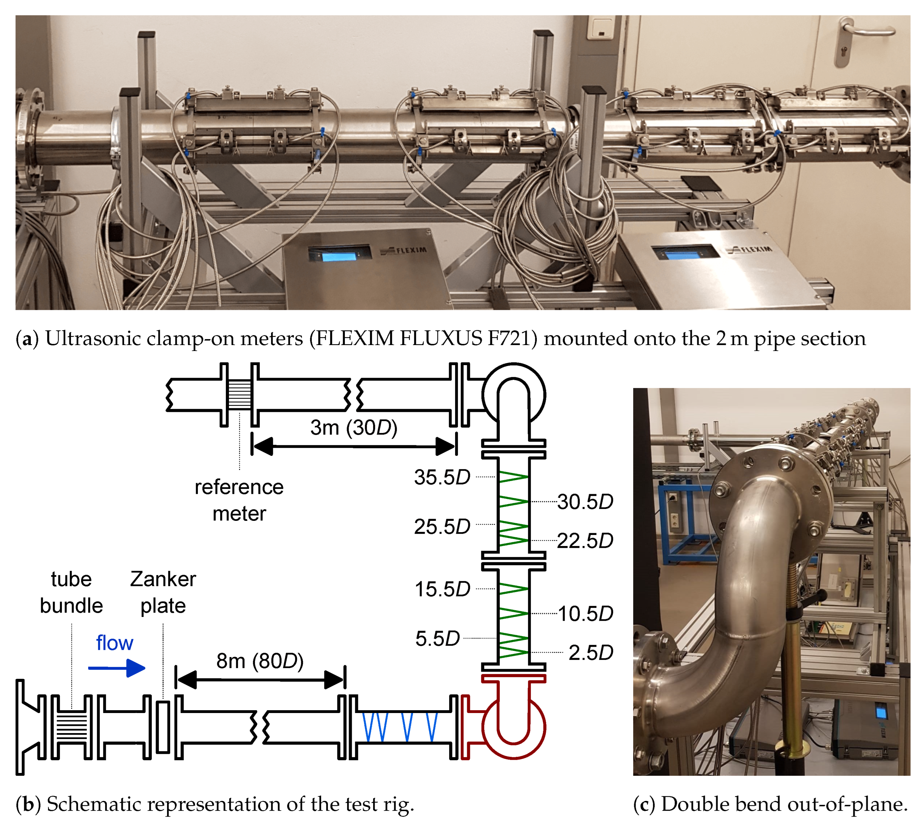
2.1. Measurement Setup

Clamp-on measurements were performed at the long-term ultrasonic and laser measurement facility (LULA) at the national metrology institute of Germany (PTB). A schematic representation of the test rig, the double bend out-of-plane, and the installation of the ultrasonic meters are depicted in Figure 1.

2.1.1. Flow Conditions

Measurements were taken at a water temperature of 30 °C (kinematic viscosity $\nu =0.8\times {10}^{-6} {\mathrm{m}}^2{\mathrm{s}}^{-1}$) and a flow rate of $\dot{V}=11.32 {\mathrm{m}}^3{\mathrm{h}}^{-1}$. This corresponds to a volumetric velocity of $v_{vol}=\dot{V}/A=0.4 \mathrm{m}{\mathrm{s}}^{-1}$ (where A is the pipe cross-section) and a friction velocity of $u_{\tau }=2.06\times {10}^{-2} \mathrm{m}{\mathrm{s}}^{-1}$, a Reynolds number of $Re=v_{vol}·D/\nu =5\times {10}^4$, and a friction Reynolds number of $R{e}_{\tau }=u_{\tau }·D/\nu =1288$.

2.1.2. Test Rig

In the configuration illustrated in Figure 1b, LULA provides measurement sections for the investigation of fully developed flow conditions and disturbed flow conditions downstream of a double bend out-of-plane. The flow rate control was realized by means of an electromagnetic reference meter (KROHNE WATERFLUX 3070) that was calibrated at the gravimetric heat meter calibration facility at the PTB. Its combined relative uncertainty and degrees of freedom (${\mathrm{dof}}_i$) at a Reynolds number of 5 × 10⁴ are given by $u_r({\dot{V}}_{ref})=7.74\times {10}^{-4}$ and ${\mathrm{dof}}_i=83$ (Straka [17]). All pipes and bends were constructed in the nominal diameter DN 100 with an internal diameter (D) of $100.0$ $\mathrm{m}$$\mathrm{m}$ ($\pm 50 \mathsf{\mu }\mathrm{m}$) and a wall roughness $R_a\approx 5 \mathsf{\mu }\mathrm{m}$, which corresponded to a dimensionless roughness parameter $k{s}^{+}\approx 0.7$. It can therefore be considered as hydraulically smooth; compare to e.g., Gersten [18]. To minimize the flange offset, they were connected by centering rings with a sliding fit tolerance of 40 $\mathsf{\mu }$$\mathrm{m}$. The double bend depicted in Figure 1c consisted of two identical welded elbow fittings with a curvature radius ($R_c$) of $142.5$ $\mathrm{m}$$\mathrm{m}$ ($R_c/D=1.425$). The measurement section downstream had a length of 4 $\mathrm{m}$, which corresponded to $40D$. To ensure fully developed flow conditions, the measurement section upstream of the double bend was preceded by a flow conditioning unit, which combined a pipe reducer (159 mm to 100 mm) with a tube bundle straightener and a Zanker plate according to ISO 5167-1 [19], see Straka et al. [20]. For investigations of fully developed flow conditions, the free inlet length added up to 8 $\mathrm{m}$ ($80D$), see Figure 1b. Similarly, the double bend was preceded by a straight inlet section of 10 $\mathrm{m}$ ($100D$).

2.1.3. Clamp-On Meters

Throughout the measurement campaign, a total of eight clamp-on meters (FLEXIM FLUXUS F721) were permanently mounted onto a 2 $\mathrm{m}$ pipe section, see Figure 1a. The meters were positioned at four locations along the pipe axis (z) and two angular orientations ($\phi$) at 18° and 108°. For the determination of the calibration factors, this unit was installed both in the first and second half of the measurement section downstream of the double bend, resulting in $N_z=8$ downstream locations with normalized distances ($z/D$) of 2.5, 5.5, 10.5, 15.5, 22.5, 25.5, 30.5 and 35.5. In each half, the pipe was rotated around the pipe axis by 45°, resulting in additional angular orientations of 63° and 153°. With $N_{\phi }=4$, the total number of measurement positions was given by $N_z·N_{\phi }=32$.

2.2. Ultrasonic Flow Rate Measurements

As illustrated in Figure 2a, the ultrasonic clamp-on meter measured a transit time difference ($\Delta t$) between the upstream and downstream signals transmitted and received by a pair of transducers A and B. Using the delay time $t_0$, the transit time at zero flow $t_{tr}$ and the path-geometry factor $K_g$, a path velocity proportional to $\Delta t$ was determined by

$$v_{path}=K_g·\frac{\Delta t}{2(t_{tr}-t_0)}.$$

(1)

As a constant of proportionality, $K_g$ has the unit of velocity. In general, volume flow rates ($\dot{V}$) are determined as $\dot{V}=A·v_{vol}$. Applied to the ultrasonic flow rate measurement using $v_{path}$, $\dot{V}$ is calculated as

$$\dot{V}=A·\underset{K_p}{\underbrace{K_u·K_d}}·v_{path}.$$

(2)

In the equation, $K_p$ represents the combined fluid mechanical calibration factor that accounts for the fact that $v_{path}$ does not comply with the volumetric velocity $v_{vol}$. For the implementation within the meter, it is useful to split $K_p$ into $K_u$ and $K_d$, representing the correction for a fully developed (undisturbed) turbulent flow and a particular flow disturbance, respectively. Values for $K_u$ can be determined experimentally or estimated using a theoretical velocity profile, e.g., the semi-analytical approach from Gersten and Herwig [21]. For the ultrasonic clamp-on meter in the reflection mode, the theoretical range of $K_u$ is from 0.75 for the laminar flows to 1 for the infinitely large Reynolds numbers in a perfectly smooth pipe. In practical applications, $K_u$ typically ranges between 0.88 and 0.98 in the turbulent regime. $K_d$, on the other hand, can typically range between 0.8 and 1.2, mainly depending on the particular flow disturbance, its downstream distance, and angular orientation towards the meter.

For the current setup, the expanded relative uncertainty of the clamp-on meters with respect to the determination of $\dot{V}$ under fully developed flow conditions is roughly estimated as $U_r(\dot{V})\approx 1\%(k=2)$; see Appendix A.1.

Figure 2. (a) Schematic illustration of an ultrasonic flow meter in the reflection mode using the transit time difference method. Source: Straka et al. [22] (CC BY 4.0). (b) Implementation of the measuring principle in the velocity field provided by the CFD simulation.

Figure 2. (a) Schematic illustration of an ultrasonic flow meter in the reflection mode using the transit time difference method. Source: Straka et al. [22] (CC BY 4.0). (b) Implementation of the measuring principle in the velocity field provided by the CFD simulation.

2.3. Derivation of the Calibration Factors

When $K_d$ is determined experimentally, this approximation is hereinafter referred to as $K_{d.E}$. Device independent values of $K_{d.E}$ were obtained by comparing the results from two separate experiments. At first, the clamp-on flow meters were exposed to fully developed flow conditions, see Figure 1b. In the second experiment, the flow meters were installed downstream of the double bend. In each measurement, the combined calibration factor $K_p$ was determined by comparing the flow rate provided by the ultrasonic flow meter ($\dot{V}$) and the reference meter of the test rig (${\dot{V}}_{ref}$) according to

$$K_p=\frac{{\dot{V}}_{ref}}{\dot{V}}.$$

(3)

From the first measurement series, $K_u$ can directly be determined from Equation (3) because, under fully developed conditions, $K_d$ equals one and, thus, $K_p=K_u$. From the second measurement series, $K_{d.E}$ can then be extracted by first calculating $K_p$ according to Equation (3) under disturbed flow conditions and then dividing it by $K_u$ according to

$$K_{d.E}=\frac{K_p}{K_u}.$$

(4)

At every measurement position, $K_p$ is calculated as the arithmetic means of three consecutive measurements, each taken within a time interval of 20 $\min$. Note that most of the input quantities for $\dot{V}$ included in Equation (2) remain constant during the measurement campaign. As a result, they can be neglected in the uncertainty analysis for $K_{d.E}$. As opposed to an individual uncertainty evaluation for $K_p$ or $K_u$, the impact of $u_r(\dot{V})$ is thus significantly reduced, see Appendix A.2.

2.4. Measurement Uncertainty

The uncertainty associated with the experimental determination of the calibration factors $K_{d.E}$ is calculated in accordance with the GUM [1]. In Section 4, it will be used for the validation of the virtual measurements and evaluation of the simulation uncertainty.

2.4.1. Combined Uncertainty $u_c\left(K_{d.E}\right)$

In its primary form, the model equation for the combined relative measurement uncertainty $u_{c,r}\left(K_{d.E}\right)$ derived from Equation (4) is given by

$$u_{c,r}^2\left(K_{d.E}\right)=u_r^2\left(K_u\right)+u_r^2\left(K_p\right).$$

(5)

For the uncertainty evaluation, the terms on the right side of Equation (5) must be divided into manageable components. A detailed description of the individual uncertainty contributions is included in Appendix A.2. For the validation of the simulation results in Section 4, the combined (absolute) measurement uncertainty $u_c\left(K_{d.E}\right)=u_{c,r}\left(K_{d.E}\right)·K_{d.E}$ is used. Throughout the measurement positions, $u_c\left(K_{d.E}\right)$ ranges from 1.50 × 10⁻³ to 3.33 × 10⁻³. These variations are largely due to the strongly location-dependent uncertainty components associated with the angular and downstream alignment as well as the reproducibility of the individual sensors, see Appendix A.2.

2.4.2. Expanded Uncertainty $U\left(K_{d.E}\right)$

As usual, in metrology, uncertainties are multiplied by a coverage factor $k\approx 2$ to obtain a confidence interval of 95.45%. This results in the expanded measurement uncertainty given by $U\left(K_{d.E}\right)=k·u_c\left(K_{d.E}\right)$ and requires the specification of the effective degrees of freedom (${\mathrm{dof}}_{eff}$). As recommended in the GUM [1], ${\mathrm{dof}}_{eff}$ is calculated by using the Welch–-Satterthwaite equation, given by

$${\mathrm{dof}}_{eff}=u_c^2·{\left[\sum _{i=1}^N\frac{u_i^4}{{\mathrm{dof}}_i}\right]}^{-1},$$

(6)

where $u_i$ and ${\mathrm{dof}}_i$ represent the individual uncertainty components of $u_c\left(K_{d.E}\right)$ and their associated degrees of freedom. Using ${\mathrm{dof}}_{eff}$ and the required confidence interval of 95.45%, k can be obtained from the inverse function of the Student’s t-distribution. A representative calculation example for $z/D=35.5$ and $\phi =18°$ is presented in Appendix A.2,

Table A1. Measurement uncertainty evaluation for $K_{d.E}=1.027$ at $z/D=35.5$ and $\phi =18°$.

Part	Description	Symbol	Relative Standard Uncertainty ${\mathit{u}}_{\mathit{i}}$	Relative Variance ${\mathit{u}}_{\mathit{i}}^2$	Proportion of Variance in [%]	Degrees of Freedom ${\mathbf{dof}}_{\mathit{i}}$
$u_r\left(K_u\right)$	Reproducibility	$u_r\left(K_{u,rep}\right)$	1.03 × 10−3	1.06 × 10−6	22.45	∞
	Reference flow rate	$u_r({\dot{V}}_{ref})$	7.74 × 10−4	5.99 × 10−7	12.67	82
	Repeatability	$u_r\left(\overline{K_u}\right)$	4.78 × 10−4	2.28 × 10−7	4.83	2
	Temperature effects	$u_r\left(K_{u,T}\right)$	1.70 × 10−4	2.89 × 10−8	0.61	29
$u_r\left(K_p\right)$	Reproducibility	$u_r\left(K_{u,rep}\right)$	1.03 × 10−3	1.06 × 10−6	22.45	∞
	Reference flow rate	$u_r({\dot{V}}_{ref})$	7.74 × 10−4	5.99 × 10−7	12.67	82
	Angular alignment	$u_r\left(K_{p,\phi }\right)$	7.22 × 10−4	5.21 × 10−7	11.03	9999
	Repeatability	$u_r\left(\overline{K_p}\right)$	7.13 × 10−4	5.08 × 10−7	10.76	2
	Downstream distance	$u_r\left(K_{p,z}\right)$	3.01 × 10−4	9.06 × 10−8	1.92	9999
	Temperature effects	$u_r\left(K_{u,T}\right)$	1.70 × 10−4	2.89 × 10−8	0.61	29
	Combined relative variance $u_{c,r}^2\left(K_{d.E}\right)$			4.73 × 10−6	100.00
	Combined relative standard uncertainty $u_{c,r}\left(K_{d.E}\right)$			2.17 × 10−3
	Effective degrees of freedom ${\mathrm{dof}}_{eff}$			136
	Coverage factor k for the confidence level of 95.45%			2.02
	Expanded relative uncertainty $U_r\left(K_{d.E}\right)$			4.39 × 10−3

. Throughout the measurement positions, $U\left(K_{d.E}\right)$ ranges from 3.05 × 10⁻³ to 6.66 × 10⁻³ ($k\approx 2$). All values are depicted in Figure 3b.

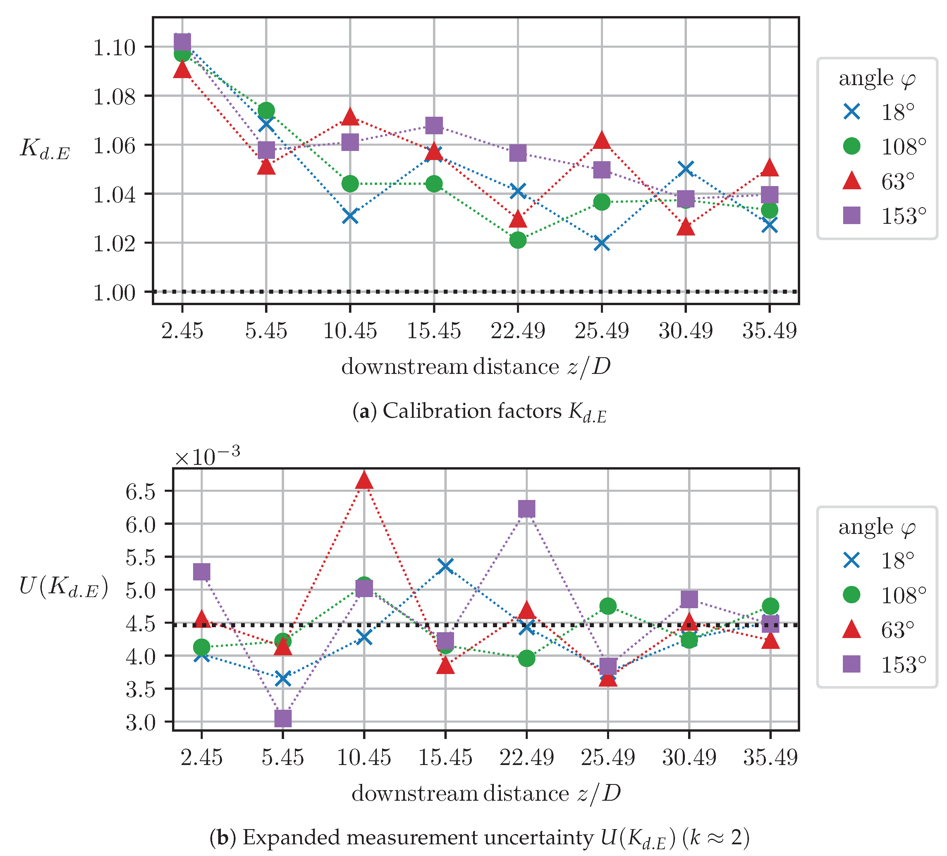
2.5. Experimental Results

The experimental results of $K_{d.E}$ at the 32 measurement positions are depicted in Figure 3a. It can be noticed that the magnitude of $K_{d.E}$ tends to decrease with growing distance to the double bend out-of-plane, although the value corresponding to fully developed flow conditions ($K_{d.E}=1$) is clearly not reached at $z/D=35.5$. Furthermore, a strong angular dependency can be detected. Thus, an interpolation between the measurement positions does not appear to be meaningful.

3. Simulation-Based Determination of Calibration Factors

The current section deals with the realization of the virtual ultrasonic clamp-on measurements. This includes a description of the simulation setup and the implementation of the measuring principle that allows a simulation-based determination of $K_d$. In analogy to the experimental terminology, the approximation of $K_d$ obtained by means of a virtual meter is referred to as $K_{d.S}$. Since the selection of the turbulence model represents the largest source of modeling errors, a variety of different turbulence models are investigated. Using today’s state-of-the-art Reynolds-averaged Navier-Stokes (RANS) models often results in poor predictions of complex flows, while scale-resolving approaches, such as large eddy simulations (LES), remain unfeasible for industrial applications. In between, hybrid RANS-LES models represent a means of combining comparatively low modeling errors and reasonable computing times. Simulation results are presented for the Spalart–Allmaras RANS and hybrid SBES-SST models. Apart from an examination of $K_{d.S}$ throughout the computational domain, an analysis of both axial and secondary velocity profiles is presented. Three different numerical uncertainties and the uncertainty due to the time averaging intervals are evaluated within a series of verification studies. Finally, the measurement and simulation results, $K_{d.S}$ and $K_{d.E}$, are compared.

3.1. Simulation Setup

Simulations were performed with the commercial software package ANSYS Fluent 2020 R1 using the pressure-based solver. Meshes for the double bend geometry and adjacent pipe sections were created with ANSYS ICEM CFD 2020 R1.

3.1.1. Turbulence Modeling

Steady-state simulations were performed with a variety of different RANS models. These included the standard k-$ϵ$ (Launder and Spalding [23]), realizable k-$ϵ$ (Shih et al. [24]), standard k-$\omega$ (Wilcox [25]), and SST k-$\omega$ (Menter [26]) models from the group of two-equation eddy-viscosity models and the one-equation Spalart–Allmaras model (Spalart and Allmaras [27]). Furthermore, three different Reynolds stress models were tested. Convergence could be achieved with the linear pressure–strain (Launder and Shima [28]) and Stress-$\omega$ (Wilcox [25]) models, whereas the quadratic pressure–strain model (Speziale et al. [29]) failed in this regard. Transient simulations with hybrid RANS-LES models were carried out with the stress-blended eddy simulation (SBES) model (Menter [30]) and the detached eddy simulation (DES) model (Spalart et al. [31]). Each was set up with both the realizable k-$ϵ$ and the SST k-$\omega$ RANS models. Low-Reynolds corrections were enabled for the k-$\omega$-based models. Apart from that, all RANS models were used in accordance with their default settings and constants in ANSYS Fluent 2020 R1. For SBES, the location-dependent blending function specified in Straka et al. [32] with a modified constant of $a=100$ as well as the Smagorinsky–Lilly sub-grid model (Smagorinsky [33]) with $C_S=0.025$ was used.

3.1.2. Solver Settings

Transient simulations were run with a time step size of $7.5$ $\mathrm{m}$$\mathrm{s}$. Following an initial adaptation period of 8000 time steps (60 s), the instantaneous velocity fields were averaged over 16,000 time steps (120 s). Further solution methods are listed in

Table 1. Applied solution methods and residuals in ANSYS Fluent 2020 R1.

	Hybrid RANS-LES	RANS
Pressure-Velocity Coupling	SIMPLE	Coupled
Discretization schemes
Temporal	Bounded Second-order Impl.	—
Spatial
Diffusion	Central differencing	Central differencing
Momentum	Central differencing	Second-order upwind
Pressure	Second-order	Second-order
Gradient	Green-Gauss cell-based	Least-Squares cell-based
Turbulent quantities	First-order upwind	Second-order upwind
Scaled residuals
Continuity, velocities	1 × 10−5	1 × 10−15
Turbulent quantities	1 × 10−4	1 × 10−15

.

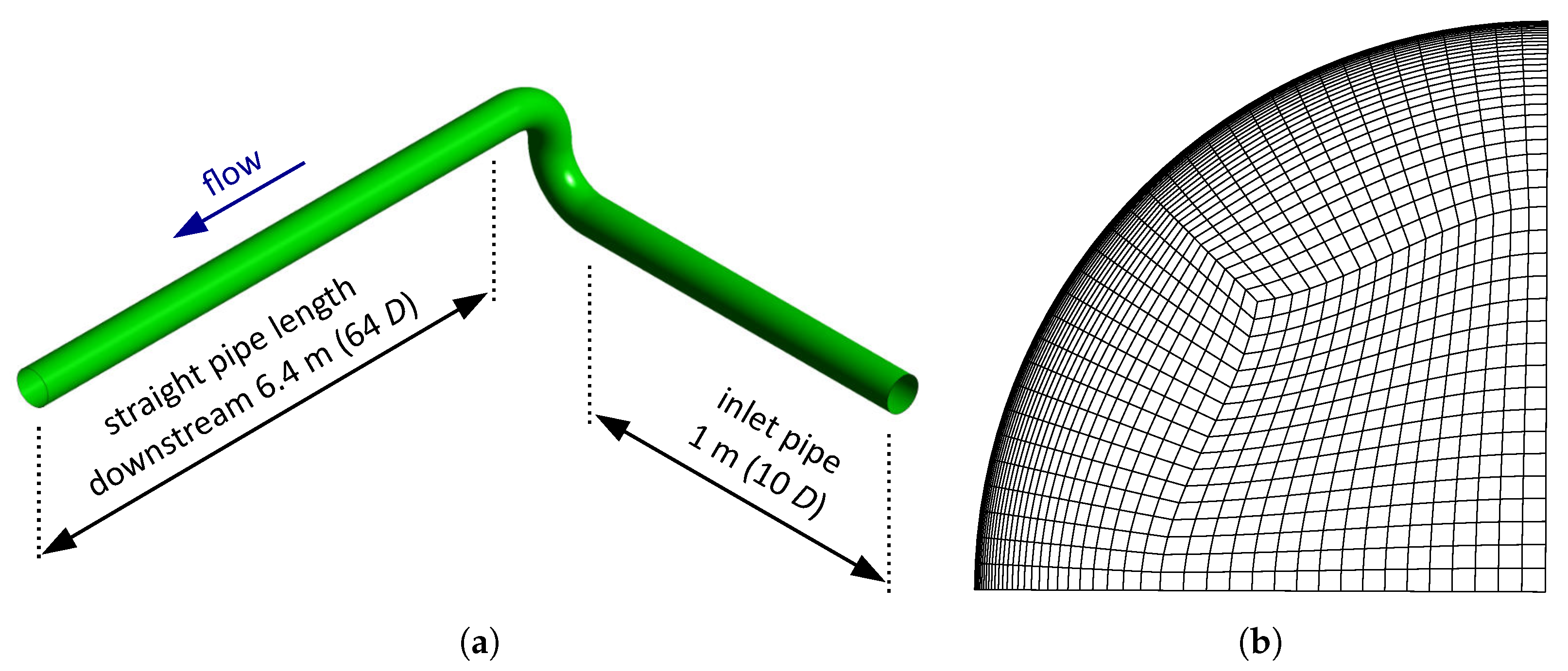
3.1.3. Geometry and Meshing

As illustrated in Figure 4a, the computational domain consists of a straight pipe section of $1.0$ $\mathrm{m}$ ($10D$), a double bend, and a subsequent pipe section of $6.4$ $\mathrm{m}$ ($64D$). The hexahedral mesh has an O-grid structure depicted in Figure 4b, which is swept along the pipe axis. Two mesh versions were used for the hybrid RANS-LES and RANS simulations. With 136 and 45 cells in the circumferential and radial direction, a non-dimensional wall distance of $y^{+}\approx 1.0$, and 43 cells per diameter in the streamwise direction, the mesh versions for the hybrid simulations have ≈1.64 × 10⁷ cells. For RANS, the streamwise grid resolution in the straight pipe sections decreased towards the inlet and outlet from 43 to 17 cells per diameter using an exponential growth rate, resulting in a reduced mesh size of ≈9.50 × 10⁶ cells.

3.1.4. Boundary Conditions

For all simulations, a fully developed velocity distribution and turbulence quantities from a precursor RANS simulation with either the SST-k-$\omega$ or standard k-$ϵ$ model were utilized at the inlet boundary. In the transient simulations, the vortex method (Mathey et al. [34]) with 250 vortex points was applied to create velocity fluctuations. Furthermore, a no-slip condition and the zero diffusion flux outflow condition were used at the pipe wall and outlet boundaries, respectively.

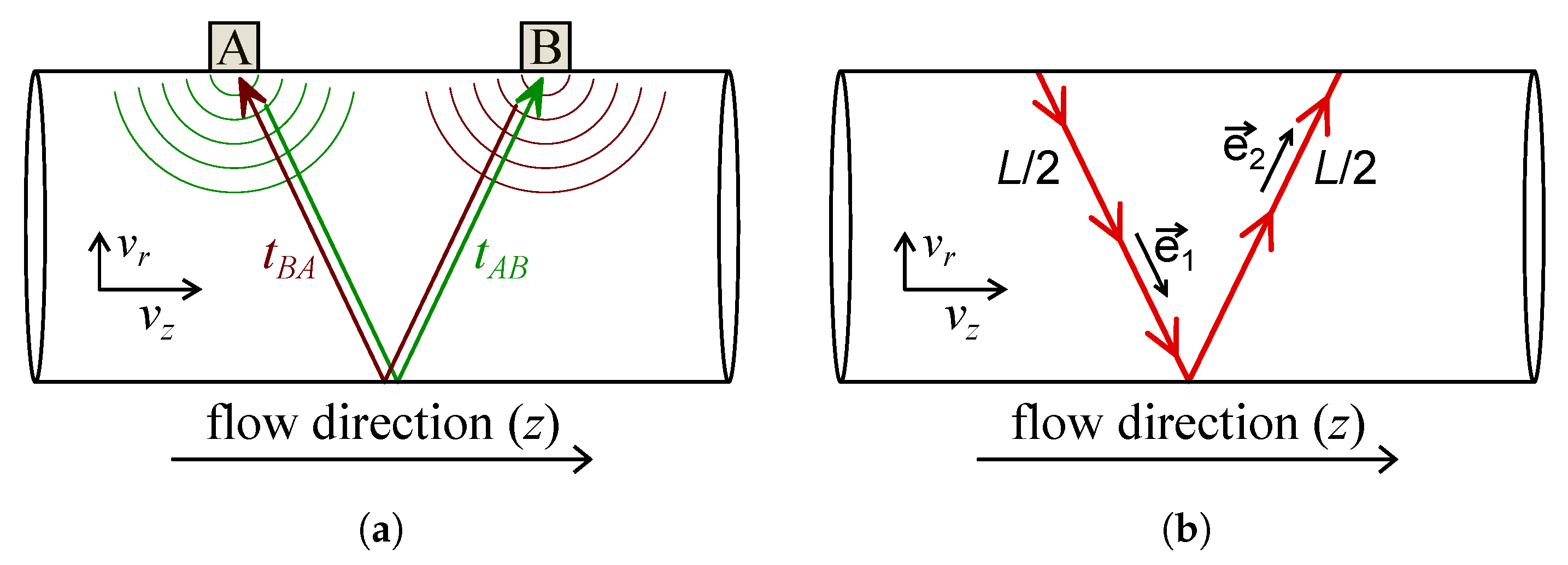
3.2. Implementation of the Measuring Principle

Similar to the experimental determination of $K_{d.E}$, $K_{d.S}$ was derived by means of the path velocity $v_{path}$. Yet, in contrast to the transit time measurement of the clamp-on meters, $v_{path}$ was calculated from the simulation results as the average velocity along the ultrasonic path geometry in the velocity field $\overrightarrow{v}$, according to

$$v_{path}=\frac{1}{L{e}_z}\left({\int }_0^{L/2}\overrightarrow{v}·\overrightarrow{e_1}\mathrm{d}l+{\int }_0^{L/2}\overrightarrow{v}·\overrightarrow{e_2}\mathrm{d}l\right),$$

(7)

where L is the length of the V-shaped ultrasonic path and $\overrightarrow{e_1},\overrightarrow{e_2}$ are the unit vectors of the two path sections, see Figure 2b. $K_{d.S}$ can be calculated by comparing the path velocities of an undisturbed reference profile and the disturbed velocity profiles according to

$$K_{d.S}=\frac{v_{path.u}}{v_{path.d}}.$$

(8)

Evaluating the fully developed profile obtained from a separate simulation of a straight pipe using the SBES-SST model yields $v_{path.u}=1.082·v_{vol}$. Since this value varied only slightly for the different turbulence models, it was used for all simulations.

3.3. Simulation Results

Results are presented for the Spalart–Allmaras and SBES-SST turbulence models. Since the simulations provide the flow field in the whole 3D domain, $K_{d.S}$ was accessible at any angular orientation and downstream distance. Flow profiles were examined to explain the specific characteristics in the measurement and simulation results.

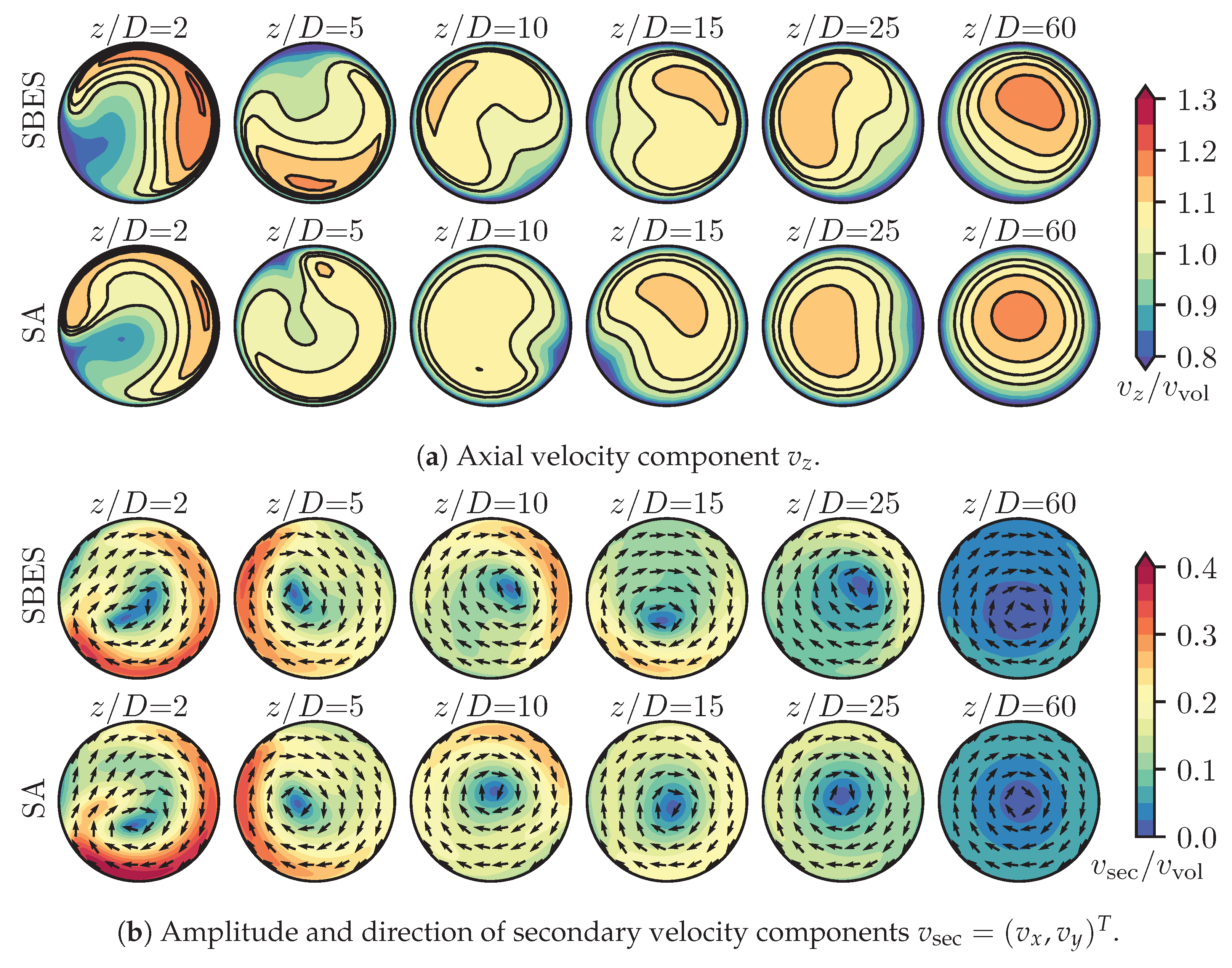
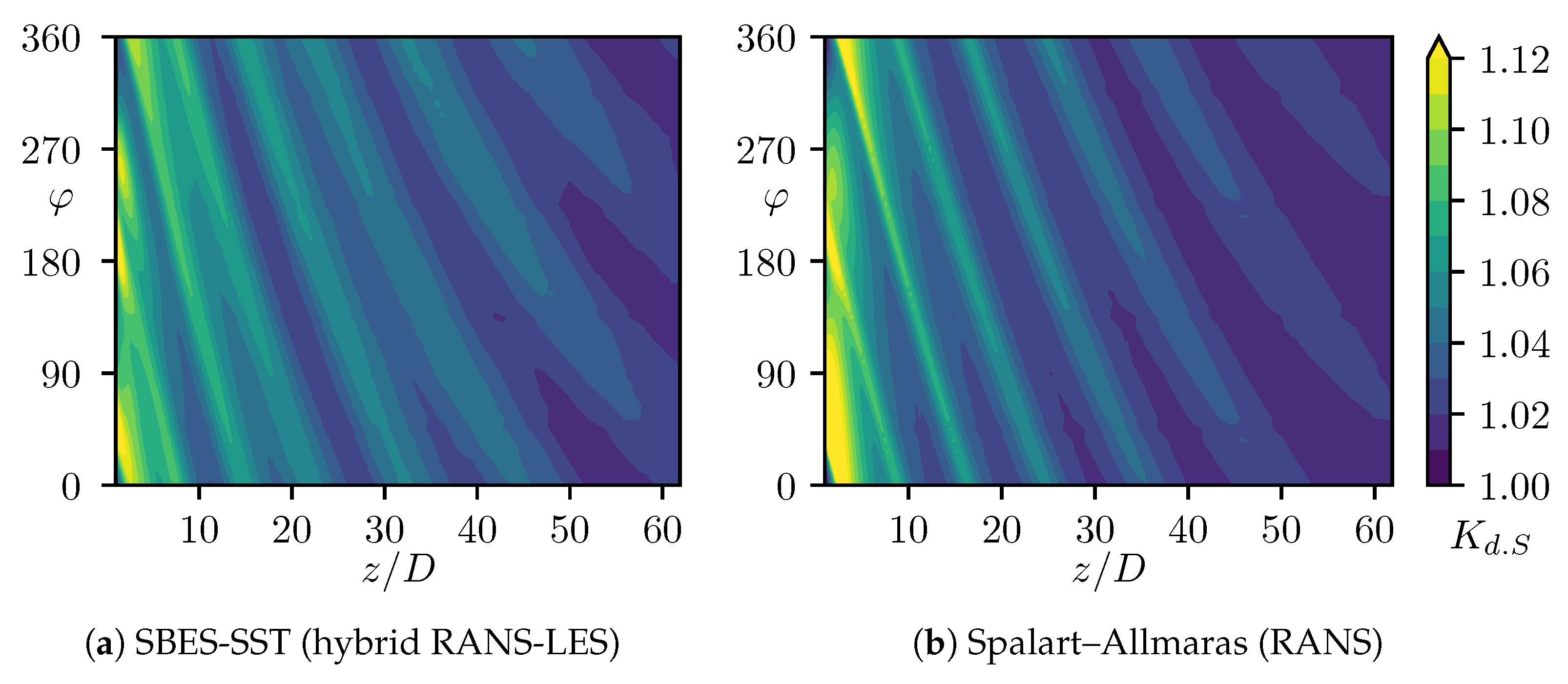
3.3.1. Spatial Distribution

Figure 5 shows that $K_{d.S}$ propagates throughout the domain in a wave-like manner. Its frequencies and amplitudes continuously diminished with increasing distance to the double bend. Yet at the maximum distance of $64D$, the flow disturbance was not fully subsided. Furthermore, the wavefronts did not run parallel to the vertical axis. This explains the angular dependency of the measurement data observed in Figure 3. While the qualitative development of $K_{d.S}$ was predicted similarly by both models, the specific arrangement of the wave crests, as well as their phases and magnitudes, were different.

3.3.2. Velocity Profiles

A velocity profile is defined as the velocity distribution over the pipe cross-section at a particular downstream position. Fully developed pipe flows are characterized by a symmetrical distribution of the time-averaged axial profile and the absence of secondary components. Velocity profiles downstream of the double bend, as predicted by the SBES-SST and Spalart–Allmaras model, are depicted in Figure 6. Throughout the domain, the axial profiles show a radial displacement of the core velocity region towards the pipe wall. In general, asymmetry can be connected to the angle-dependent fluctuations observed for $K_d$, as the average velocity along the individual ultrasonic paths ($v_{path}$) varies accordingly. In comparison to fully developed conditions, the axial profiles have overall flatter shapes. As a result, $v_{path}$ takes on comparatively smaller values and $K_d$ is thus consistently larger than 1. In addition to the deformation, the axial velocity profiles describe a helical movement around the pipe axis in the clockwise direction. This correlates with the single vortex structure (swirl) present in the secondary flow, see Figure 6b. The rotation is the reason for the wave-like patterns of $K_{d.S}$ in Figure 5, i.e., a rotation of 360° corresponds to the length between two adjacent wave crests.

Comparing the two turbulence models, it is noticeable that the shapes of the axial profiles, especially in the near-field range up $z/D=5$, are qualitatively different. At $z/D=60$, the progression towards the fully developed state is much further advanced in the case of the RANS model. This is consistent with the comparatively lower values of $K_{d.S}$ in the far-field range observed in Figure 5. As for the secondary velocity profiles in Figure 6b, the swirling velocity is slightly higher in the case of the SBES-SST model. As a result, there is a noticeable phase shift between the axial profiles in Figure 6a.

3.4. Calculation Verification

Numerical uncertainties and the uncertainties due to the time-averaging interval were evaluated as part of a calculation verification. All contributions were combined in the calculation uncertainty $u_{cal}\left(K_{d.S}\right)$, which will be used for the comparison between $K_{d.E}$ and $K_{d.S}$ in Section 3.5.

3.4.1. Numerical Uncertainties

Three independent studies covering the overall spatial discretization ($u_{disc}$), wall-normal grid resolution at the wall ($u_{wall}$), and iterative convergence within time steps ($u_{iter}$) were conducted. In the case of the transient simulations, $u_{disc}$ also included temporal discretization. As for RANS, $u_{iter}$ was neglected, given that scaled residuals of 1 × 10⁻¹⁵ were used. In each study, simulations with three different refinement levels were evaluated. Their parameters are listed in

Table 2. Variable parameters in the verification studies regarding the numerical uncertainties.

Uncertainty		Variable Parameter (s)	Refinement Level
Error Source	Symbol		1	2	3
spatial & temporal discretization	$u_{disc}$	cells on circumference	120	136	160
		streamwise cells/diameter	35	43	50
		cells in radial direction	41	45	51
		time step size [ms]	10	8	7
spatial discretization wall-normal direction	$u_{wall}$	wall-normal distance $y^{+}$	1.0	0.5	0.2
iterative convergence within time steps	$u_{iter}$	scaled momentum residual	${10}^{-5}$	${10}^{-6}$	${10}^{-7}$

.

The Richardson extrapolation is a common method used to calculate and correct numerical errors, see, e.g., Roache [16]. This approach requires an asymptotic convergence for a parameter, such as the grid size when the level of refinement is increased. In case of oscillatory convergence, Richardson extrapolation fails, and errors cannot be derived or corrected. As an alternative, Stern et al. [14] suggest stating numerical uncertainties as one-half of the difference between the highest and lowest values of the acquired target variable. Given that $K_{d.S,max}$ and $K_{d.S,min}$ represent the maximum and minimum within a verification study, the local numerical uncertainty component is thus calculated as

$$u_{num,local}=\frac{1}{2}·\left(K_{d.S,max}-K_{d.S,min}\right).$$

(9)

A representation for the entire domain is obtained by calculating the arithmetic mean over $\phi \in [0,2\pi )$ and $z/D\in [2,20]$ in steps of $\pi /60$ and 1, respectively. In all studies for both models, the different solutions show an oscillatory convergence. Thus, $u_{disc}$, $u_{wall}$, and $u_{iter}$ are estimated in accordance with Equation (9). Results are listed in

Table 3. Calculation uncertainties associated with the simulation-based determination of $K_d$.

Uncertainty		Turbulence Model
Related to	Symbol	SBES-SST (Hybrid)	Spalart–Allmaras (RANS)
Time-averaging	$u_{time}$	1.32 × 10−3	–
Grid & time step size	$u_{disc}$	1.65 × 10−3	2.73 × 10−3
Wall-normal distance	$u_{wall}$	1.52 × 10−3	1.14 × 10−3
Iterative convergence	$u_{iter}$	1.13 × 10−3	–
Calculation	$u_{cal}\left(K_{d.S}\right)$	2.84 × 10−3	2.96 × 10−3
	$U_{cal}\left(K_{d.S}\right)$	5.68 × 10−3	5.91 × 10−3

.

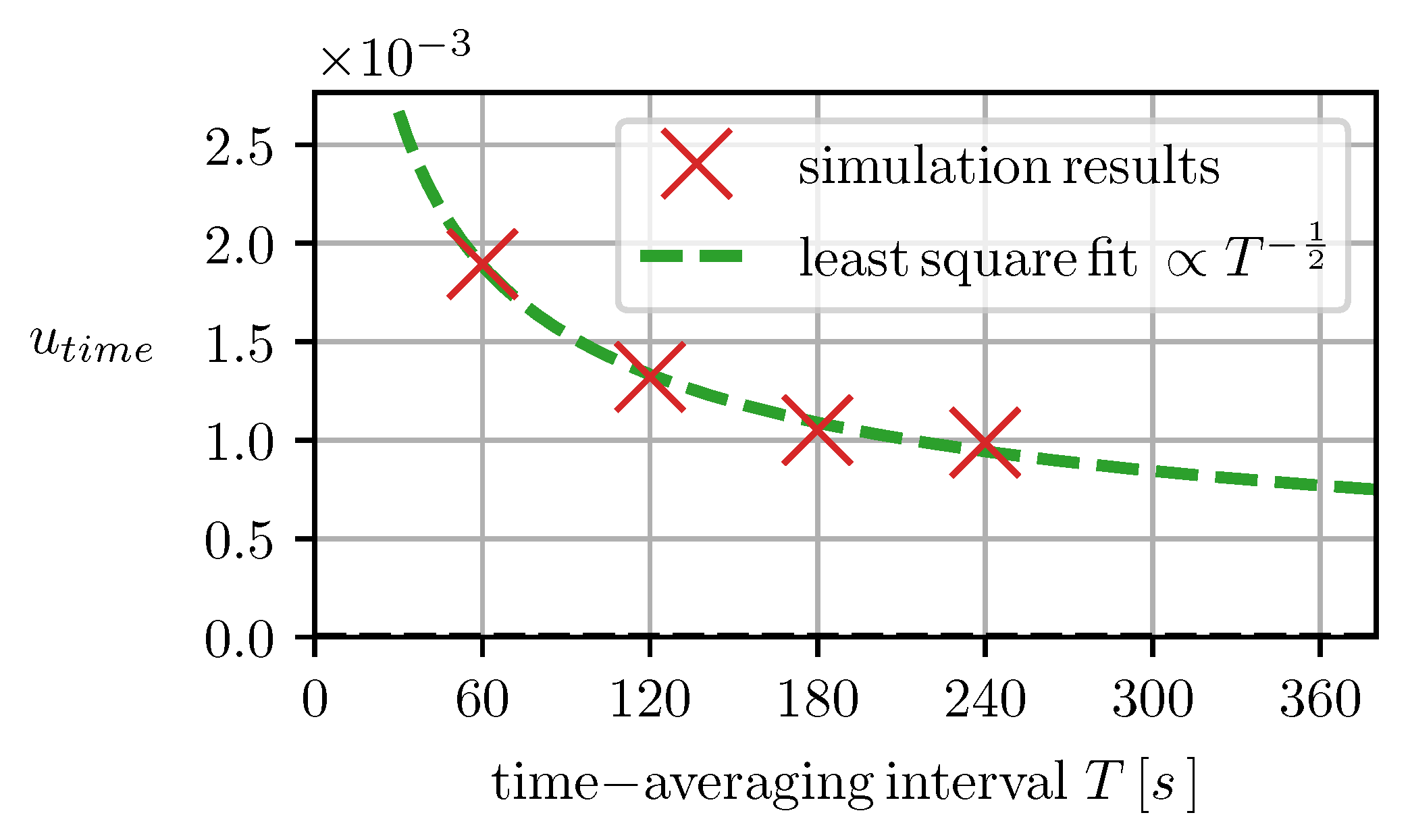
3.4.2. Time-Averaging Uncertainty

Temporal fluctuations in turbulent flows are typically not represented by fluid mechanical calibration factors, meaning that $K_d$ is designed to be independent of time. Nonetheless, the influence of low-frequency turbulent fluctuations is generally not negligible for practical simulation times. The determination of $K_{d.S}$ as an average over a finite time interval T in a transient simulation therefore involves a source of uncertainty, herein referred to as $u_{time}$. Its presence in the simulation setup is connected to the physically correct yet arbitrary state of the initial conditions in the domain and the velocity fluctuations at the inlet boundary at $t=0$. While $u_{time}$ decreases with an increasing simulation time, it should always be considered in transient simulations.

Local values of $u_{time}$ are estimated using the empirical standard deviation $s\left(K_{d.S}\right)$ from a total of 10 individual simulation runs with different starting solutions. This approach is similar to a repeatability test in an experimental uncertainty analysis. Analogous to the numerical uncertainties, a representation for the entire domain is obtained by calculating the arithmetic mean. For T = 120 s, as utilized in the setup for the SBES-SST model, $u_{time}$ is determined as 1.32 × 10⁻³. Other values corresponding to 60 s, 180 s and 240 s are depicted in Figure 7. It is found that the time-dependent development of the uncertainty contribution can be approximated with $u_{time}=a/\sqrt{T·1/\mathrm{s}}$, where $a=1.46\times {10}^{-2}$ was determined by a least-squares fit.

3.4.3. Calculation Uncertainty

It is assumed that the simulation parameters addressed in the verification studies were independent. Thus, the components can be combined in the calculation uncertainty

$$u_{cal}^2\left(K_{d.S}\right)=u_{disc}^2+u_{wall}^2+u_{iter}^2+u_{time}^2.$$

(10)

In the case of the steady-state simulations, only $u_{disc}$ and $u_{wall}$ were included in $u_{cal}\left(K_{d.S}\right)$. Since a confidence interval of 95.45% was targeted, the expanded calculation uncertainty $U_{cal}\left(K_{d.S}\right)=k·u_{cal}\left(K_{d.S}\right)$ with $k=2$ was introduced. Values of $u_{cal}\left(K_{d.S}\right)$ and $U_{cal}\left(K_{d.S}\right)$ calculated for the SBES-SST and Spalart–Allmaras turbulence models are included in Table 3 and Figure 8. It was found that $u_{disc}$ determined for the RANS model exceeded that of the hybrid model by a factor of $\approx 1.7$, whereas for $u_{wall}$, it was the other way around. In combination with the additional components evaluated for the SBES-SST simulation, $u_{cal}\left(K_{d.S}\right)$ was nearly identical for both models. For a more detailed analysis regarding the impacts of different mesh sizes, time step sizes, and other parameters on the simulation results of double bends, see Straka [17]. Regarding the progression of $u_{time}$ in Figure 7, increasing T from 120 $\mathrm{s}$ to 180 $\mathrm{s}$ reduces the uncertainty by ≈20%. This decreases $u_{cal}\left(K_{d.S}\right)$ in the SBES-SST simulation by only ≈2.5% and, thus, does not justify the additional computing time.

In comparison to the fluctuation range of $K_{d.S}$ in Figure 5, $U_{cal}\left(K_{d.S}\right)$ was smaller by a factor of ≈20. This can be regarded as an indication of a sufficiently high quality of the simulation setup. Nonetheless, the inability to eliminate numerical errors means that the validation experiment following the verification studies not only evaluates modeling errors in particular, but the errors arising from the simulation as a whole.

Figure 8. Comparison between $K_{d.E}\pm U\left(K_{d.E}\right)$ and $K_{d.S}$, including the expanded calculation uncertainty $U_{cal}\left(K_{d.S}\right)$ determined for the hybrid SBES-SST and Spalart–Allmaras (SA) RANS model. In contrast to $U\left(K_{d.S}\right)$, $U_{cal}\left(K_{d.S}\right)$ does not cover the modeling uncertainty (compare Figure 9). $U\left(K_{d.E}\right)$ and $U_{cal}\left(K_{d.S}\right)$ are represented by error bars and bands, respectively.

Figure 8. Comparison between $K_{d.E}\pm U\left(K_{d.E}\right)$ and $K_{d.S}$, including the expanded calculation uncertainty $U_{cal}\left(K_{d.S}\right)$ determined for the hybrid SBES-SST and Spalart–Allmaras (SA) RANS model. In contrast to $U\left(K_{d.S}\right)$, $U_{cal}\left(K_{d.S}\right)$ does not cover the modeling uncertainty (compare Figure 9). $U\left(K_{d.E}\right)$ and $U_{cal}\left(K_{d.S}\right)$ are represented by error bars and bands, respectively.

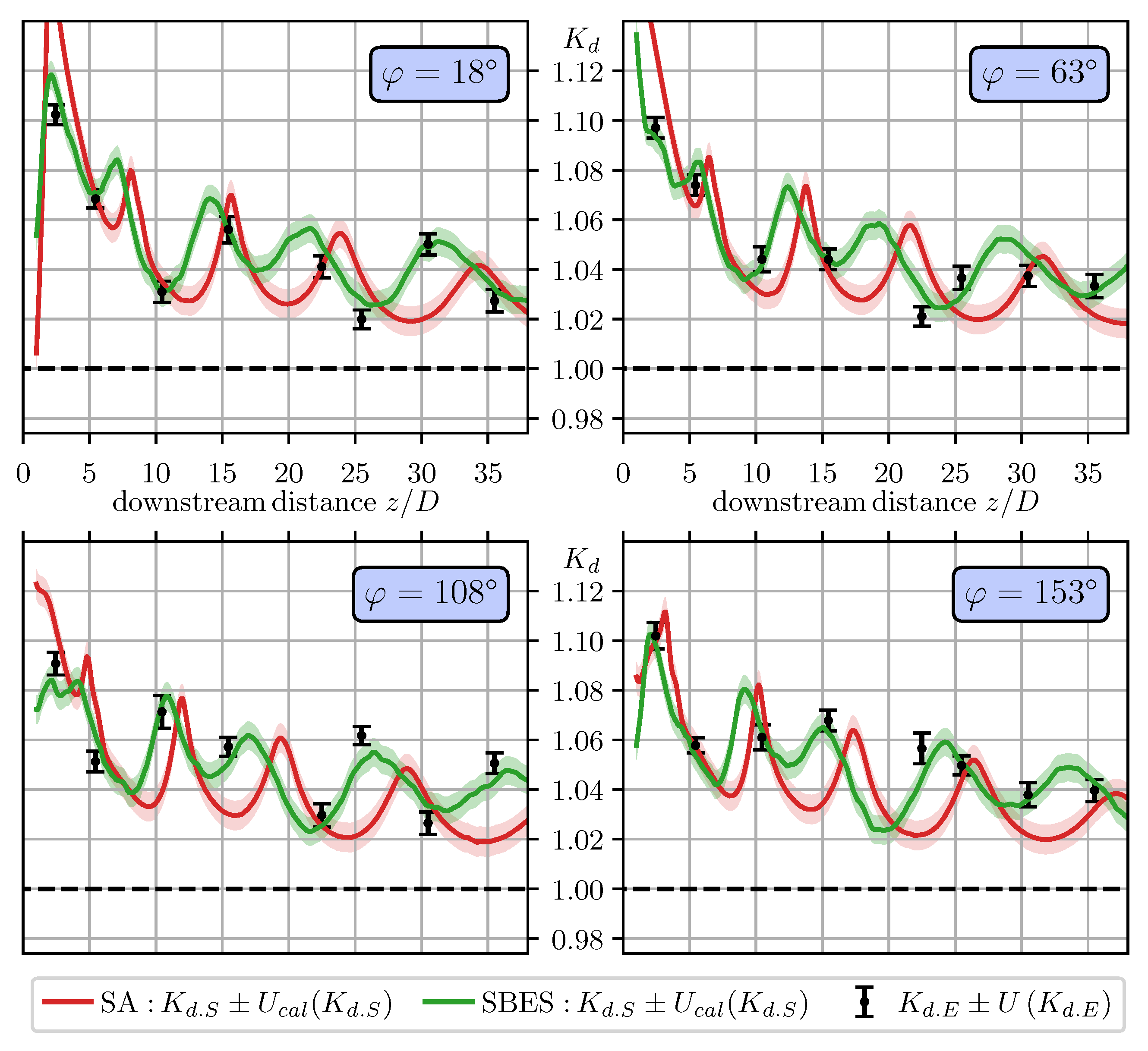
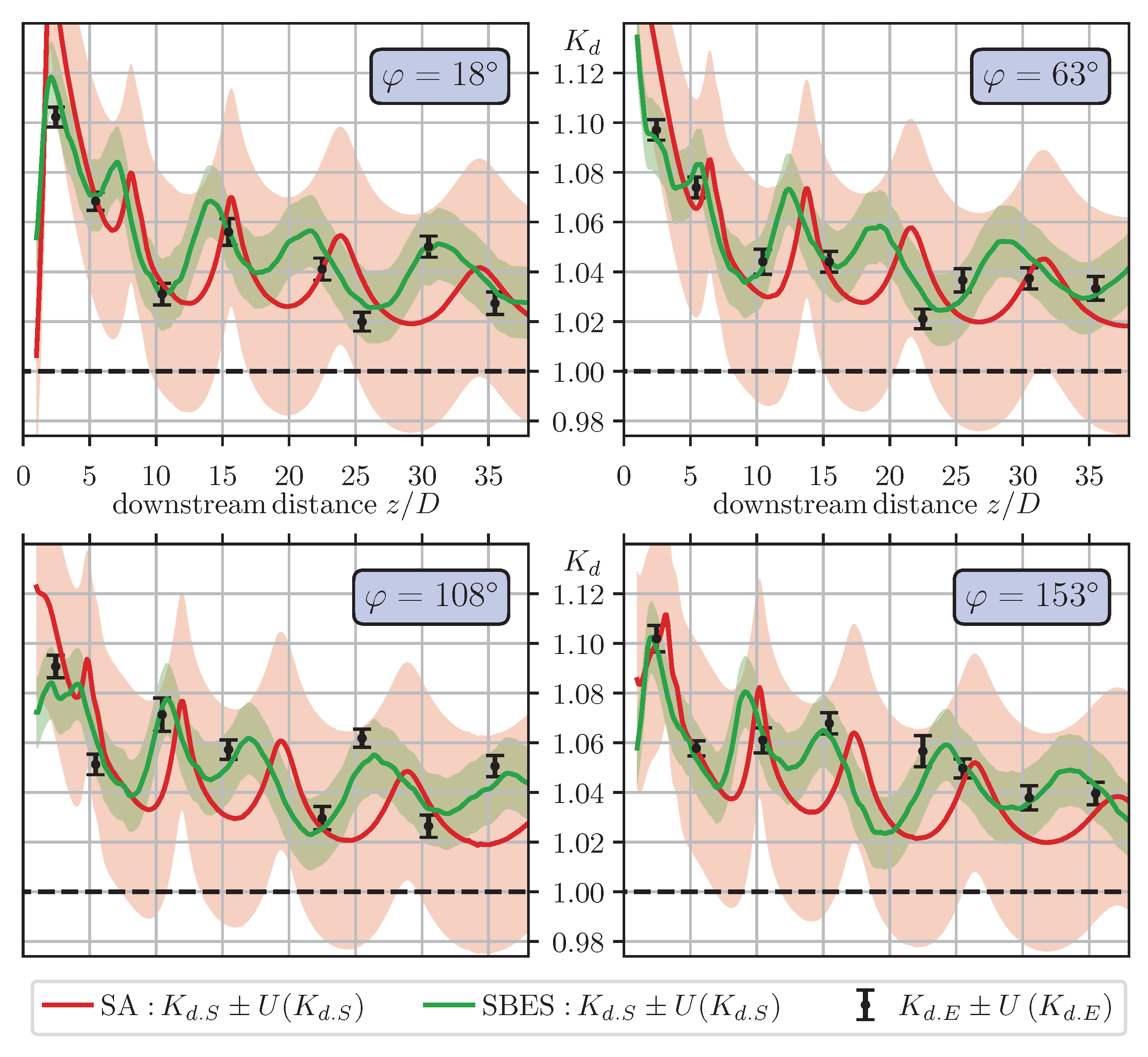
3.5. Comparison with Experimental Data

A comparison between $K_{d.E}$ and $K_{d.S}$ over the downstream distance is presented in Figure 8. As observed in Figure 5, there is a significant phase shift between $K_{d.S}$ as predicted by the two turbulence models, visible at all angular orientations. In general, the predictions obtained from the simulation with the SBES-SST model are in better agreement with the measurement data. Nonetheless, $K_{d.E}\pm U\left(K_{d.E}\right)$, in part, lie on the edges or even fall outside the specified uncertainty band of $K_{d.S}$, even though $U_{cal}\left(K_{d.S}\right)$ describes a confidence interval of 95.45%. This implies that the predominant components in the overall uncertainty budget (especially in the RANS simulation) must stem from modeling errors, most evidently simplifications of the turbulence model.

4. Simulation Uncertainty

This section contains the novel approach to assess the expanded simulation uncertainty $U\left(K_{d.S}\right)$ in analogy to the evaluation of measurement uncertainty according to the GUM [1]. Since the result of a virtual measurement includes an approximation of $K_d$ in the entire computational domain, $U\left(K_{d.S}\right)$ is supposed to be valid for all angular orientations and downstream positions. Its derivation is based on the magnitude and distribution of simulation errors $\delta \left(K_{d.S}\right)$ that can be calculated at the measurement positions. Given that the numerical errors could not be corrected during verification in Section 3, $\delta \left(K_{d.S}\right)$ contains all sources of errors arising from the simulation as a whole. Conditions for a correction of systematic errors and spatial patterns in the error distribution are examined. The individual concepts are illustrated for the SBES-SST model, while the results obtained for the other turbulence models are discussed in Section 4.4.

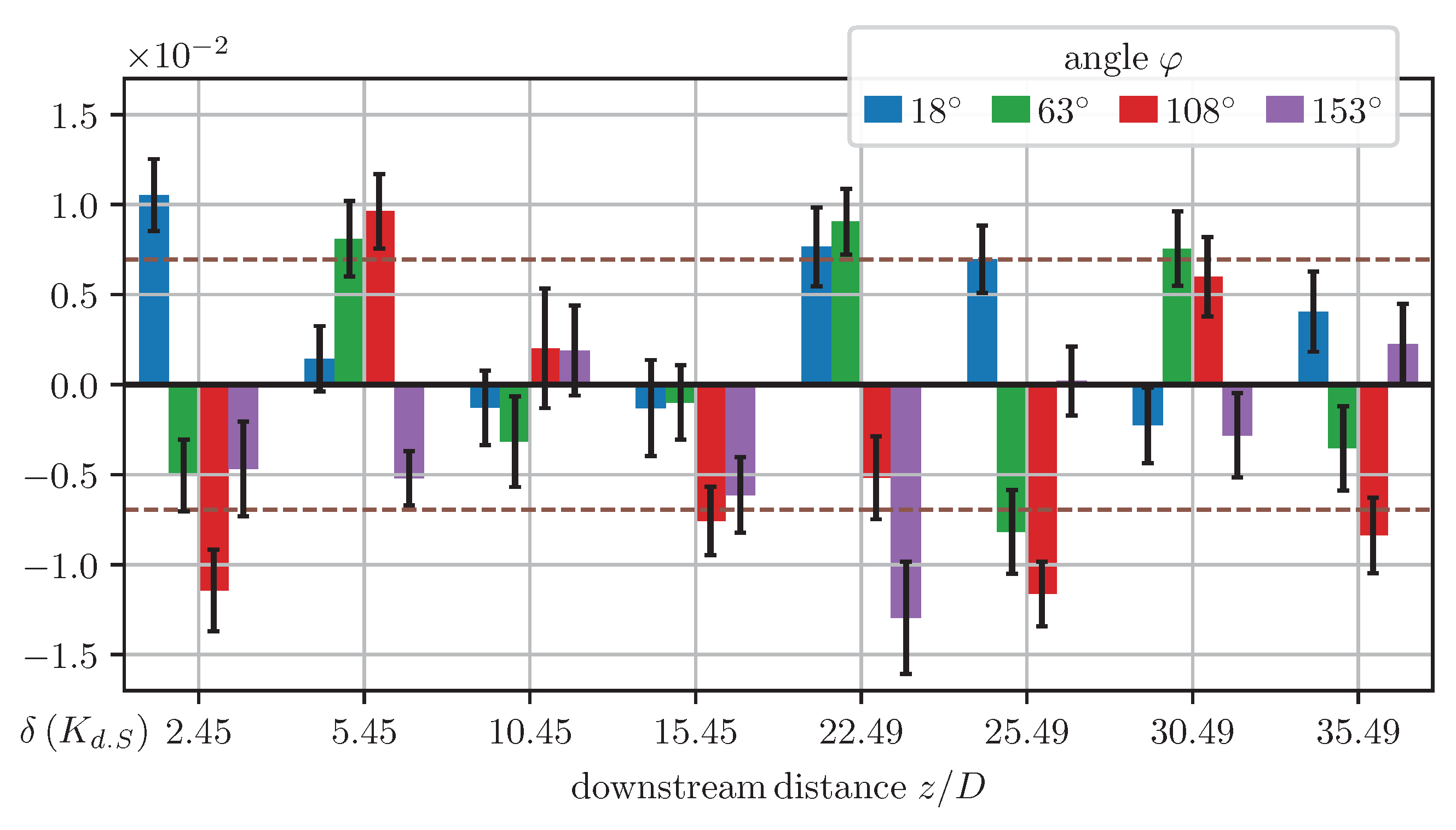
4.1. Simulation Error

A simulation error associated with a particular variable of interest is defined as the difference between the simulation result at a specific location in the computational domain and the true value. This relation also applies to measurement errors. Thus, the errors in the simulation $\delta \left(K_{d.S}\right)$ and experimental data $\delta \left(K_{d.E}\right)$, with regard to the determination of the calibration factor $K_d$, are given by

$$\begin{array}{cc}\hfill \delta \left(K_{d.S}\right)& =K_{d.S}-K_d,\hfill \end{array}$$

(11a)

$$\begin{array}{cc}\hfill \delta \left(K_{d.E}\right)& =K_{d.E}-K_d.\hfill \end{array}$$

(11b)

Equation (11a,b) cannot be solved individually, as the true value of $K_d$ is unknown. Yet by inserting Equation (11a) into (11b), $\delta \left(K_{d.S}\right)$ can be written as

$$\delta \left(K_{d.S}\right)=K_{d.S}-K_{d.E}+\delta \left(K_{d.E}\right).$$

(12)

In this form, $\delta \left(K_{d.S}\right)$ can be determined at the measurement positions with the restriction that $\delta \left(K_{d.E}\right)$ must be estimated. All values of $\delta \left(K_{d.S}\right)$ calculated from the results obtained with the SBES-SST model are depicted in Figure 10. In the figure, the errors in the experimental data $\delta \left(K_{d.E}\right)$ are represented by the combined measurement uncertainty $u_c\left(K_{d.E}\right)$. Excluding the experimental errors, the individual values of $\delta \left(K_{d.S}\right)$ ranged between −1.30 × 10⁻² and 1.05 × 10⁻².

4.2. Correction of Systematic Errors

Adapting the simulation results by eliminating systematic errors can be useful for reducing the overall simulation uncertainty. The most basic method is to remove the systematic share by subtracting the arithmetic mean of the simulation errors, such that

$$K_{d.S,corr}=K_{d.S}-\overline{\delta }\left(K_{d.S}\right)$$

(13)

represents a corrected version of $K_{d.S}$. This adjustment is only adequate if $\overline{\delta }\left(K_{d.S}\right)$ is significant. We suggest establishing significance under the condition that the absolute mean is greater than its standard error, i.e.,

$$\left|\overline{\delta }\left(K_{d.S}\right)\right|>s\left(\delta \left(K_{d.S}\right)\right)/\sqrt{N},$$

(14)

where s is the empirical standard deviation and $N=32$ is the number of measurement positions and, thus, the individual values of $\delta \left(K_{d.S}\right)$. In case of the simulation results obtained with the SBES-SST model, $\overline{\delta }=-7.63\times {10}^{-4}$ and $s=6.91\times {10}^{-3}$. Thus, $\left|\overline{\delta }\right|$ is smaller than its standard error $s/\sqrt{32}=1.22\times {10}^{-3}$. Consequently, a correction according to Equation (13) is not pursued. As for the other turbulence models investigated in this study, the condition set out in Equation (14) is fulfilled in the case of the SBES-realizable-k-$ϵ$, Spalart–Allmaras, and linear pressure–strain model (see

Table 4. Simulation uncertainty results of all turbulence models.

Turbulence Model	$\overline{\mathit{\delta }}\left({\mathit{K}}_{\mathit{d}.\mathit{S}}\right)$ Significant?	$\mathit{u}\left({\mathit{K}}_{\mathit{d}.\mathit{S}}\right)$	Coverage Factor k	$\mathit{U}\left({\mathit{K}}_{\mathit{d}.\mathit{S}}\right)$
SBES-SST [30]	no	6.96 × 10−3	2.07	1.44 × 10−2
SBES-realizable k-$ϵ$ [30]	yes	1.29 × 10−2	2.08	2.67 × 10−2
DES-realizable k-$ϵ$ [31]	no	1.42 × 10−2	2.08	2.96 × 10−2
DES-SST [31]	no	1.63 × 10−2	2.08	3.39 × 10−2
Spalart-Allmaras [27]	yes	2.10 × 10−2	2.08	4.38 × 10−2
SST k-$\omega$ [26]	no	2.35 × 10−2	2.08	4.89 × 10−2
Standard k-$\omega$ [25]	no	2.73 × 10−2	2.08	5.69 × 10−2
Linear pressure–strain [28]	yes	2.78 × 10−2	2.08	5.80 × 10−2
Standard k-$ϵ$ [23]	no	3.06 × 10−2	2.08	6.38 × 10−2
Realizable k-$ϵ$ [24]	no	3.14 × 10−2	2.08	6.55 × 10−2
Stress-$\omega$ [25]	no	3.82 × 10−2	2.08	7.95 × 10−2

).

4.3. Uncertainty Quantification

Following the specification of the simulation errors, the objective is to provide an expanded uncertainty $U\left(K_{d.S}\right)$ associated with the prediction of $K_{d.S}$ at arbitrary locations downstream of the double bend, such that the interval $\pm U\left(K_{d.S}\right)$ contains $\delta \left(K_{d.S}\right)$ with a probability of 95.45%. Since evaluating $U\left(K_{d.S}\right)$ is based on the magnitude and spatial arrangement of the simulation errors, the spatial autocorrelation was examined at first.

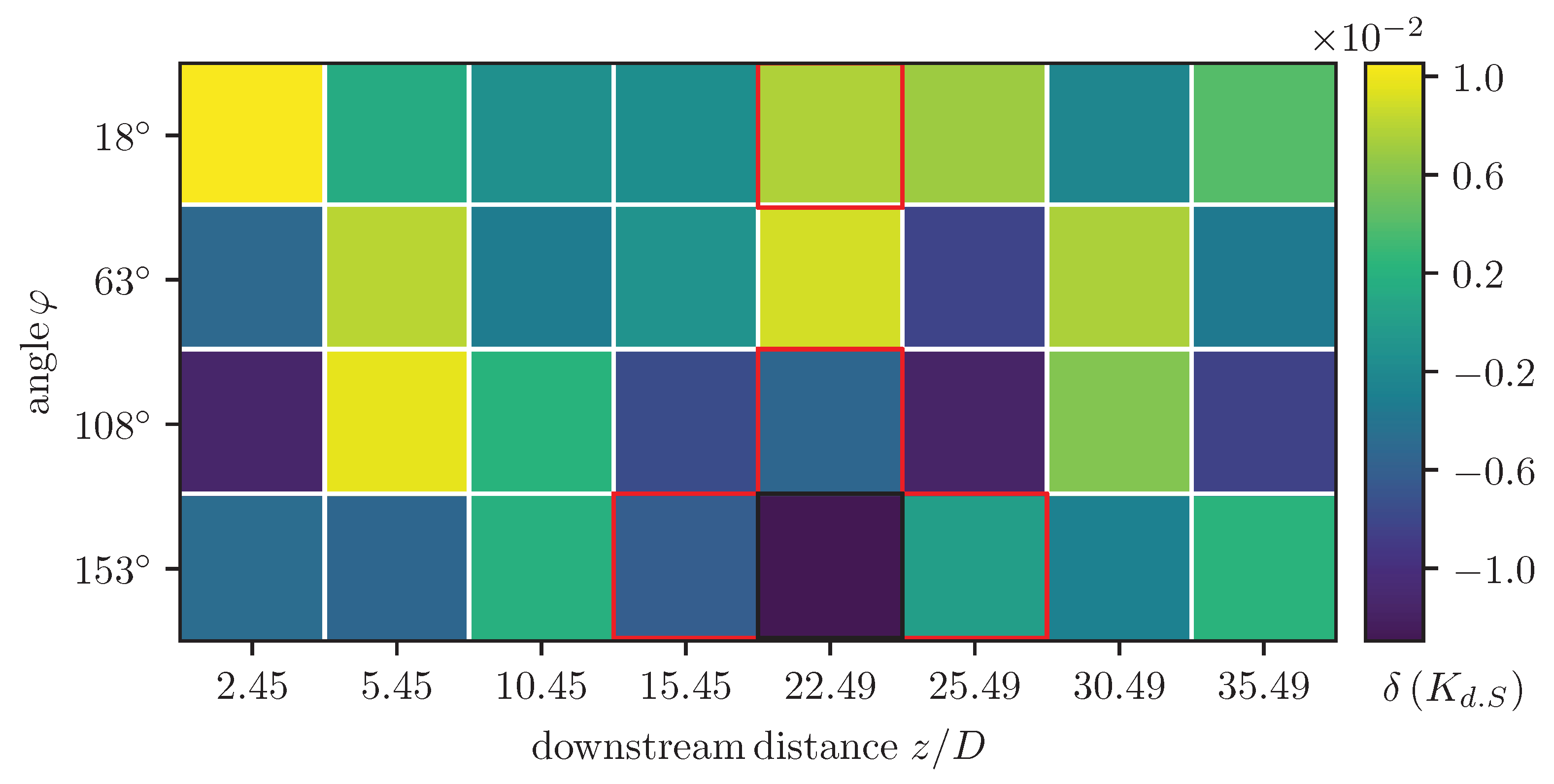
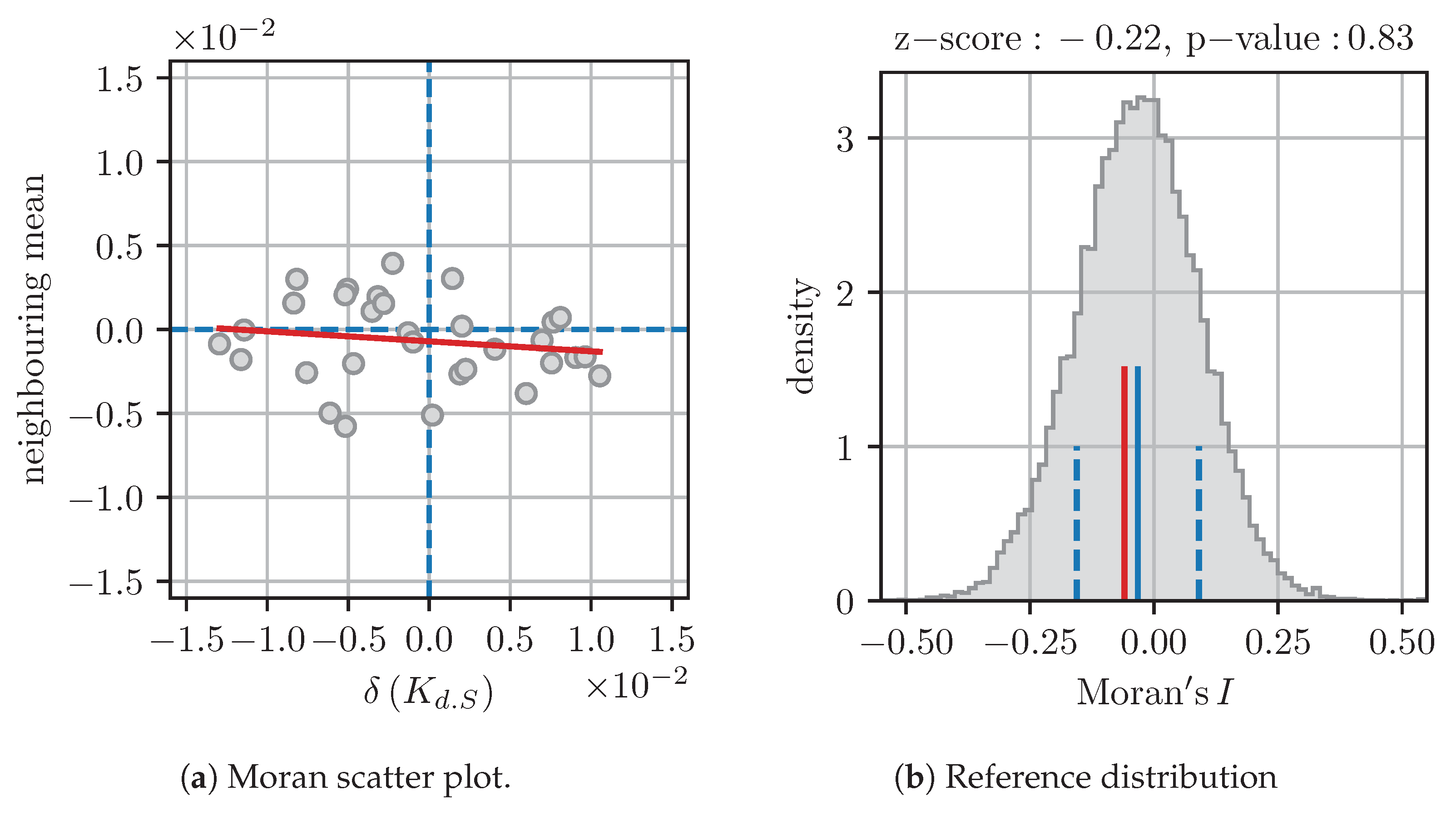
4.3.1. Spatial Autocorrelation

Clear positive correlations between $\delta \left(K_{d.S}\right)$ and the downstream distance or angular orientation towards the double bend can be used to attribute corresponding dependencies to the uncertainty. The spatial arrangement of the simulation errors in Figure 10, however, does not seem to follow any discernible pattern within the measurement range. For this reason, we assume that the simulation errors determined for the SBES-SST results can be considered as white noise, meaning that their magnitudes and signs are spatially independent. This hypothesis is confirmed through an evaluation of spatial autocorrelation using Moran’s I [35], see Appendix B. Due to the absence of patterns in the spatial distribution, the values of $\delta \left(K_{d.S}\right)$ at the measurement positions cannot be used to interpolate or extrapolate errors throughout the computational domain. Consequently, the simulation uncertainty is specified to be independent of the downstream distance and angular orientation towards the double bend.

4.3.2. Standard Uncertainty

Standard uncertainty is defined as the estimated standard deviation, which in this case is equivalent to the sample standard deviation s. If the systematic share of the simulation errors is eliminated according to Equation (13), the relative standard uncertainty representing the corrected simulation results is therefore given by

$$u\left(K_{d.S,corr}\right)=s\left(\delta \left(K_{d.S,corr}\right)\right).$$

(15)

If, on the other hand, $\overline{\delta }\left(K_{d.S}\right)$ is not significant under the condition given in Equation (13), an equivalent standard uncertainty associated with $K_{d.S}$ can be calculated according to

$$u^2\left(K_{d.S}\right)={\overline{\delta }}^2\left(K_{d.S}\right)+s^2\left(\delta \left(K_{d.S}\right)\right).$$

(16)

Equations (15) and (16) can be solved by means of a Monte Carlo simulation, where $\delta \left(K_{d.E}\right)$ is randomly sampled from a normal distribution with an expected value of $\mu =0$ and a standard deviation that corresponds to the combined measurement uncertainty $u_c\left(K_{d.E}\right)$. As for the (uncorrected) simulation results obtained with the SBES-SST model, solving Equation (16) using a Monte Carlo simulation and a total of 2 × 10⁵ trails yields $u\left(K_{d.S}\right)=6.96\times {10}^{-3}$. In case of the other turbulence models, the standard simulation uncertainty takes values up to 3.82 × 10⁻², exceeding SBES-SST by a factor of ≈$5.5$ (see Table 4). Compared to the hybrid models, the uncertainties calculated for the RANS models are consistently higher.

Since $u\left(K_{d.S}\right)$ represents a combination of many different numerical and modeling errors, it can be assumed to be approximately normally distributed. If a quantity is normally distributed with the expected value $\mathsf{\mu }$ and standard deviation $\sigma$, the interval $[\mu -\sigma ,\mu +\sigma ]$ contains ≈68.3% of the distribution. In case of the SBES-SST results, $\pm u\left(K_{d.S}\right)$ encompasses 21 out of 32 values of $\delta \left(K_{d.S}\right)$, which corresponds to ≈65.6%.

4.3.3. Expanded Simulation Uncertainty

Stating the expanded uncertainty that provides the desired level of confidence of 95.45% requires the specification of a corresponding coverage factor k. Thus, k, being the most practical option, is estimated by applying the methodology described in the GUM [1], which is based on the usage of t-distributions and degrees of freedom (${\mathrm{dof}}_{eff}$).

It is found that the solution to Equation (16) obtained by means of a Monte Carlo simulation can be approximated with an accuracy of ≈$\pm 1.5\%$ by applying the propagation of uncertainty according to

$$u^2\left(K_{d.S}\right)\approx {\tilde{u}}^2\left(K_{d.S}\right)+{\overline{u}}_c^2\left(K_{d.E}\right).$$

(17)

In the equation, ${\overline{u}}_c\left(K_{d.E}\right)$ is the arithmetic mean of $u_c\left(K_{d.E}\right)$ at the $N=32$ measurement positions. Furthermore, $\tilde{u}\left(K_{d.S}\right)$ is the solution to Equation (16) under the assumption that all experimental errors are zero. This approximation can also be applied to $u\left(K_{d.S,corr}\right)$. Considering $u\left(K_{d.S}\right)$ as a combined uncertainty allows the determination of ${\mathrm{dof}}_{eff}$ using the individual degrees of freedom (${\mathrm{dof}}_i$) and the Welch—Satterthwaite equation (Equation (6)). Regarding $\tilde{u}\left(K_{d.S}\right)$, ${\mathrm{dof}}_i$ can be connected to the number of measurements and thus, is determined as ${\mathrm{dof}}_i=N-1=31$. As for ${\overline{u}}_c\left(K_{d.E}\right)$, ${\mathrm{dof}}_i$ is determined as the arithmetic mean of ${\mathrm{dof}}_{eff}$ at the 32 measurement positions, which gives ${\mathrm{dof}}_i=613$. In case of the simulation results obtained with the SBES-SST model, Equation (6) yields ${\mathrm{dof}}_{eff}=38$. The corresponding coverage factor for a confidence interval of 95.45% using the inverse function of the Student’s t-distribution is calculated as $k=2.07$. Finally, the expanded simulation uncertainty can be stated as $U\left(K_{d.S}\right)=k·u\left(K_{d.S}\right)$ = 1.44 × 10⁻². Table 4 lists the coverage factors and expanded uncertainties obtained with the other turbulence models.

4.4. Comparison of Results for Different Turbulence Models

Table 4 includes the simulation uncertainties obtained with all turbulence models investigated in this study. Furthermore, an updated visualization of the comparison between $K_{d.E}$ and $K_{d.S}$ using $U\left(K_{d.S}\right)$ instead of $U_{cal}\left(K_{d.S}\right)$ is presented in Figure 9.

In general, better results were gained with the hybrid RANS-LES turbulence models, as the uncertainties calculated for the RANS models were consistently higher. Among the hybrids, the SBES-SST model exhibited the lowest simulation uncertainty of $U\left(K_{d.S}\right)=1.44\times {10}^{-2}$. As for RANS, the lowest uncertainty was obtained with the one-equation Spalart–Allmaras model in the amount of $U\left(K_{d.S}\right)=4.38\times {10}^{-2}$, surpassing the two-equation RANS and seven-equation Reynolds stress models. Figure 9 reveals that starting at a downstream distance of ≈$10D$, the uncertainty of the RANS model was nearly as large as the measurement error caused by the disturbance. Thus, while using the RANS model for the near-field range may be beneficial, its predictions in the far-field range are not meaningful. In contrast, the uncertainty band of the SBES-SST model still allows for a clear distinction between adjacent installation positions. It can be concluded that the higher uncertainties in case of RANS are connected to the phase shift between the axial velocity profiles illustrated in Figure 6a.

In the transient and steady-state simulations, $U\left(K_{d.S}\right)$ exceeded $U_{cal}\left(K_{d.S}\right)$ by a factor of ≈4.0 and 7.4, respectively. Similarly, if $U\left(K_{d.S}\right)$ is considered as a combined uncertainty, the associated proportion of variance of $U_{cal}$ amounts to only 12.7% in case of SBES-SST and 2.0% in the case of the Spalart–Allmaras model. This clearly suggests that the modeling errors are the dominating contributions to the overall uncertainty.

5. Discussion

In this paper, a framework for assessing the simulation uncertainty $U\left(K_{d.S}\right)$ of a virtual meter realized by means of CFD was proposed. It was conducted on the example of determining fluid mechanical calibration factors for an ultrasonic clamp-on flow meter installed downstream of a double bend out-of-plane. In conformity with the expression of measurement uncertainty according to the GUM [1], $U\left(K_{d.S}\right)$ was set as an expanded uncertainty providing a confidence interval of 95.45%. Given that the outcome of the virtual flow measurement is not an individual value but an array of equally important values, $U\left(K_{d.S}\right)$ was designed to be valid for the approximation of $K_d$ at arbitrary installation positions downstream of the disturbance. In accordance with its intended use, the virtual measurement therefore allowed for a continuous determination of calibration factors applicable to the relevant mounting positions of the real meter.

$U\left(K_{d.S}\right)$ was derived on the basis of simulation errors, which were in turn quantified as functions of the experimentally determined calibration factors $K_{d.E}$, including their corresponding uncertainties $U\left(K_{d.E}\right)$. Since, as a result, $U\left(K_{d.S}\right)$ cannot be smaller than $U\left(K_{d.E}\right)$, the considerable effort put into the determination of $K_{d.E}$ and the quantification of $U\left(K_{d.E}\right)$ can be justified. Similarly, the virtual meter complies with the requirements established for the digital metrological twin as defined by Eichstädt et al. [4], in that $K_{d.S}$ is validated by traceable measurements and $U\left(K_{d.E}\right)$ calculated according to valid standards. The large number of measurements covering the interesting range of installation positions for the meter is of course time- and cost-intensive and could thus be regarded as a disadvantage of the methodology. However, due to the simplifications and assumptions that are still required for modeling turbulent flows within a feasible time frame, it might be the only suitable way to ensure confidence in a CFD-based virtual meter that fulfills metrological standards.

In contrast to the standard verification and validation approach, where the numerical and modeling uncertainties attributed to a CFD simulation are processed one after the other, $U\left(K_{d.S}\right)$ describes the uncertainty of the virtual measurement as a whole. On the one hand, evaluating the entire simulation setup in the validation was simply due to the fact that during verification, a correction of the numerical errors by means of the Richardson extrapolation failed. On the other hand, this supports studies (such as Hosder et al. [15]) suggesting that numerical and modeling errors cannot always be separated due to potential interactions between simulation parameters. This applies in particular to transient simulations, where, e.g., a refinement of the mesh results in a resolution of smaller eddy scales and a reduction of the modeled turbulent viscosity. In that regard, achieving grid independence is only possible if the requirements for a direct numerical simulation are fulfilled. Nonetheless, verification studies as conducted in this paper represent a means to detect crucial parameters and minimize sources of errors in the simulation setup. As an alternative to the Richardson extrapolation, numerical errors were incorporated in the expanded calculation uncertainty $U_{cal}\left(K_{d.S}\right)$ and compared to $U\left(K_{d.S}\right)$. It was concluded that the modeling errors must be the dominating contributions to the overall uncertainty, especially in the RANS simulation.

Different modeling approaches and commonly used turbulence models were used for the simulation setup of the virtual flow meter. Based on $U\left(K_{d.S}\right)$, the comparison demonstrated clear superiority of the hybrid RANS-LES turbulence models over the industry standard RANS. Among the hybrids, the best results were achieved with the SBES-SST model. In practical applications, however, the accuracy of a model has to be balanced against the available computing powers. While $U\left(K_{d.S}\right)$ calculated for the Spalart–Allmaras RANS model exceeded SBES-SST by a factor of ≈3, the computation time required for the transient simulation of the double bend was roughly 100 times higher. This can become impractical, especially if parameter studies with a great number of geometrical variations or Reynolds numbers are involved. On the other hand, it was demonstrated that a virtual measurement carried out with a RANS model is meaningless if its associated uncertainty is in the order of the meter error it is intended to compensate. Despite its comparatively high computing times, a clear recommendation can therefore be made for the use of hybrid RANS-LES turbulence models. As for RANS, the deficiency was related to an inferior prediction regarding the phase position of the axial velocity profiles. Since this is a flow phenomenon typically attributed to double bend out-of-plane configurations, the trade-off between accuracy and computational costs has to be re-evaluated for different flow disturbances.

While the simulation uncertainty calculated in this study may be an appropriate estimation for similar geometries, it is at this point limited to the double bend out-of-plane with a curvature radius of $R_c/D=1.425$. To accomplish a transferability to other double bend configurations, we suggest further validation studies in the relevant range of curvature radii and distances between the bends. In that case, a small number of measurement positions may be sufficient, provided a similar simulation setup is used. The approach for quantifying simulation uncertainties as presented here can further be extended to different flow disturbances or other CFD-based virtual flow meter designs. If this incorporates additional dominant flow phenomena, such as flow separation, we recommend a sufficiently large number of experimental data for the validation and a comparison between different turbulence models. Apart from flow applications, the proposed method could further be applied to other fields in metrology, where the evaluation of the overall uncertainty describing a virtual measurement is linked to a validation experiment.

References

1. Joint Committee for Guides in Metrology. Evaluation of Measurement Data—Guide to the Expression of Uncertainty in Measurement; International Bureau of Weights and Measures (BIPM): Sèvres, France, 2008. [Google Scholar]
2. Joint Committee for Guides in Metrology. Evaluation of Measurement Data—Supplement 1 to the “Guide to the Expression of Uncertainty in Measurement”—Propagation of Distributions Using a Monte Carlo Method; International Bureau of Weights and Measures (BIPM): Sèvres, France, 2008. [Google Scholar]
3. Joint Committee for Guides in Metrology. Evaluation of Measurement Data—Supplement 2 to the “Guide to the Expression of Uncertainty in Measurement”—Extension to Any Number of Output Quantities; International Bureau of Weights and Measures (BIPM): Sèvres, France, 2011. [Google Scholar]
4. Eichstädt, S.; Elster, C.; Härtig, F.; Heißelmann, D.; Kniel, K.; Wübbeler, G. VirtMet—Applications and Overview; International Workshop on Metrology for Virtual Measuring Instruments and Digital Twins, Physikalisch-Technische Bundesanstalt (PTB): Berlin, Germany, 2021. [Google Scholar]
5. Poroskun, I.; Rothleitner, C.; Heißelmann, D. Structure of digital metrological twins as software for uncertainty estimation. J. Sens. Sens. Syst. 2022, 11, 75–82. [Google Scholar] [CrossRef]
6. Grieves, M.; Vickers, J. Digital Twin: Mitigating Unpredictable, Undesirable Emergent Behavior in Complex Systems. In Transdisciplinary Perspectives on Complex Systems: New Findings and Approaches; Kahlen, F.J., Flumerfelt, S., Alves, A., Eds.; Springer International Publishing: Cham, Switzerland, 2017; pp. 85–113. [Google Scholar] [CrossRef]
7. Fuller, A.; Fan, Z.; Day, C.; Barlow, C. Digital Twin: Enabling Technologies, Challenges and Open Research. IEEE Access 2020, 8, 108952–108971. [Google Scholar] [CrossRef]
8. Wright, L.; Davidson, S. How to tell the difference between a model and a digital twin. Adv. Model. Simul. Eng. Sci. 2020, 7, 13. [Google Scholar] [CrossRef]
9. Le Maître, O.P.; Knio, O.M. Spectral Methods for Uncertainty Quantification; Springer: Dordrecht, The Netherlands, 2010. [Google Scholar]
10. Schmelter, S.; Fiebach, A.; Model, R.; Bär, M. Numerical prediction of the influence of uncertain inflow conditions in pipes by polynomial chaos. Int. J. Comput. Fluid Dyn. 2015, 29, 411–422. [Google Scholar] [CrossRef]
11. Schmelter, S.; Fiebach, A.; Weissenbrunner, A. Polynomial chaos for uncertainty quantification in flow simulations for metrological applications. TM Tech. Mess. 2016, 83, 71–76. [Google Scholar] [CrossRef]
12. Weissenbrunner, A.; Fiebach, A.; Schmelter, S.; Bär, M.; Thamsen, P.; Lederer, T. Simulation-based determination of systematic errors of flow meters due to uncertain inflow conditions. Flow Meas. Instrum. 2016, 52, 25–39. [Google Scholar] [CrossRef] [Green Version]
13. American Institute of Aeronautics and Astronautics (Ed.) AIAA Guide for the Verification and Validation of Computational Fluid Dynamics Simulations; American Institute of Aeronautics and Astronautics: Reston, VA, USA, 1998. [Google Scholar] [CrossRef]
14. Stern, F.; Wilson, R.; Coleman, H.; Paterson, E. Comprehensive Approach to Verification and Validation of CFD Simulations—Part 1: Methodology and Procedures. J. Fluids Eng. 2001, 123, 792. [Google Scholar] [CrossRef]
15. Hosder, S.; Grossman, B.; Watson, L.; Mason, W. Observations on CFD Simulation Uncertainties. In Proceedings of the 9th AIAA/ISSMO Symposium on Multidisciplinary Analysis and Optimization, Atlanta, GA, USA, 4–6 September 2002. [Google Scholar] [CrossRef]
16. Roache, P.J. Quantification of uncertainty in computational fluid dynamics. Annu. Rev. Fluid Mech. 1997, 29, 123–160. [Google Scholar] [CrossRef] [Green Version]
17. Straka, M. Vergleich Realer und Synthetisch Generierter Strömungszustände in Rohrleitungen Mittels Numerischer und Laseroptischer Verfahren. Ph.D. Thesis, Technische Universität Berlin, Berlin, Germany, 2021. [Google Scholar] [CrossRef]
18. Gersten, K. Fully Developed Turbulent Pipe Flow. In Fluid Mechanics of Flow Metering; Merzkirch, W., Ed.; Springer: Berlin, Germany, 2005; pp. 1–22. [Google Scholar]
19. ISO 5167-1:2003; Measurement of Fluid Flow by Means of Pressure Differential Devices Inserted in Circular Cross-Section Conduits Running Full—Part 1: General Principles and Requirements. International Organization for Standardization (ISO): Geneva, Switzerland.
20. Straka, M.; Eichler, T.; Koglin, C.; Rose, J. Similarity of the asymmetric swirl generator and a double bend in the near-field range. Flow Meas. Instrum. 2019, 70, 101647. [Google Scholar] [CrossRef]
21. Gersten, K.; Herwig, H. Strömungsmechanik. Grundlagen der Impuls-, Wärme- und Stoffübertragung aus Asymptotischer Sicht, 1st ed.; Springer: Braunschweig/Wiesbaden, Germany, 1992. [Google Scholar] [CrossRef]
22. Straka, M.; Koglin, C.; Eichler, T. Segmental orifice plates and the emulation of the 90°- bend. TM Tech. Mess. 2019, 87, 18–31. [Google Scholar] [CrossRef] [Green Version]
23. Launder, B.; Spalding, D. The numerical computation of turbulent flows. Comput. Methods Appl. Mech. Eng. 1974, 3, 269–289. [Google Scholar] [CrossRef]
24. Shih, T.H.; Liou, W.W.; Shabbir, A.; Yang, Z.; Zhu, J. A new k-ϵ eddy viscosity model for high reynolds number turbulent flows. Comput. Fluids 1995, 24, 227–238. [Google Scholar] [CrossRef]
25. Wilcox, D.C. Turbulence Modeling for CFD, 2nd ed.; DCW Industries, Inc.: La Canada, CA, USA, 1998. [Google Scholar]
26. Menter, F.R. Two-Equation Eddy-Viscosity Turbulence Models for Engineering Applications. AIAA J. 1994, 32, 1598–1605. [Google Scholar] [CrossRef] [Green Version]
27. Spalart, P.; Allmaras, S. A One-Equation Turbulence Model for Aerodynamic Flows. AIAA 1992, 439. [Google Scholar] [CrossRef]
28. Launder, B.; Shima, N. Second-moment closure for the near-wall sublayer—Development and application. AIAA J. 1989, 27, 1319–1325. [Google Scholar] [CrossRef]
29. Speziale, C.; Sarkar, S.; Gatski, T. Modelling the pressure-strain correlation of turbulence—An invariant dynamical systems approach. J. Fluid Mech. 1991, 227, 245–272. [Google Scholar] [CrossRef]
30. Menter, F. Stress-blended eddy simulation (SBES)—A new paradigm in hybrid RANS-LES modeling. In Progress in Hybrid RANS-LES Modelling; Springer: Cham, Switzerland, 2018; Volume 137, pp. 27–37. [Google Scholar] [CrossRef]
31. Spalart, P.; Jou, W.H.; Strelets, M.; Allmaras, S. Comments on the Feasibility of LES for Wings, and on a Hybrid RANS/LES Approach. In Proceedings of the Advances in DNS/LES, 1st AFOSR International Conference on DNS/LES, Ruston, LA, USA, 4–8 August 1997. [Google Scholar]
32. Straka, M.; Fiebach, A.; Koglin, C.; Eichler, T. Hybrid simulation of a segmental orifice plate. Flow Meas. Instrum. 2018, 60, 124–133. [Google Scholar] [CrossRef]
33. Smagorinsky, J. General Circulation Experiments with the Primitive Equations. Mon. Weather Rev. 1963, 91, 99–164. [Google Scholar] [CrossRef]
34. Mathey, F.; Cokljat, D.; Bertoglio, J.P.; Sergent, E. Specifications of LES inlet boundary condition using vortex method. In Proceedings of the 4th International Symposium on Turbulence, Heat and Mass Transfer, Antalya, Turkey, 12–17 October 2003. [Google Scholar]
35. Moran, P.A.P. Notes on Continuous Stochastic Phenomena. Biometrika 1950, 37, 17–23. [Google Scholar] [CrossRef] [PubMed]
36. ISO 12242; Measurement of Fluid Flow in Closed Conduits—Ultrasonic Transit-Time Meters for Liquid. International Organization for Standardization (ISO): Geneva, Switzerland, 2012.
37. Akima, H. A new method of interpolation and smooth curve fitting based on local procedures. J. ACM 1970, 17, 589–602. [Google Scholar] [CrossRef]
Figure 1. Measurement setup at the long-term ultrasonic and laser measurement facility (LULA). In (b), the blue and green V-shaped markers represent the positions of the ultrasonic meters installed upstream and downstream of the double bend, respectively.
Metrology 02 00021 g001
Figure 3. Ultrasonic clamp-on measurement results downstream of the double bend out-of-plane.
Metrology 02 00021 g003
Figure 4. (a) Double bend out-of-plane (curvature radius R c / D = 1.425 ) and adjacent pipe geometry. The length of the downstream distance is not shown to scale. (b) One-quarter of the multi-block-structured O-grid in the pipe cross-section.
Metrology 02 00021 g004
Figure 5. Calibration factor K d . S calculated from the simulation results acc. Equation (8) as a function of the angular orientation ( φ ) and downstream distance ( z / D ).
Metrology 02 00021 g005
Figure 6. Velocity profiles downstream of the double bend out-of-plane.
Metrology 02 00021 g006
Figure 7. Uncertainty contribution due to the finite length of the time-averaging interval.
Metrology 02 00021 g007
Figure 9. Comparison between K d . E ± U ( K d . E ) and K d . S , including the expanded simulation uncertainty U ( K d . S ) determined for the hybrid SBES-SST and Spalart–Allmaras (SA) RANS model. U ( K d . E ) and U ( K d . S ) are represented by error bars and bands, respectively.
Metrology 02 00021 g009
Figure 10. Simulation error δ ( K d . S ) of the SBES-SST model acc. Equation (12). Experimental errors δ ( K d . E ) are represented by the combined measurement uncertainty u c ( K d . E ) with black error bars. The brown dashed lines indicate the standard simulation uncertainty u ( K d . S ) acc. Equation (16).
Metrology 02 00021 g010