Integrated Optimization of Routing, Scheduling, Charging, and Platooning for a Mixed Fleet of Electric and Conventional Trucks

Abstract

The integration of truck platooning and electrification presents a promising avenue for improving operational efficiency and environmental sustainability in freight transportation. Realizing the energy and cost saving as well as emission reduction benefits requires a holistic design of truck routing, scheduling, and platooning strategies that account for practical operational constraints. This study investigates the integrated planning problem of routing, scheduling, and platooning for a mixed fleet of conventional trucks (CTs) and electric trucks (ETs), referred to as mixed fleet truck platooning (MFTP) problem. The MFTP incorporates charging scheduling and key operational factors, such as platooning leader–follower positioning under the battery constraints of ETs, charging station availability and capacity, and the positional configuration of trucks within a platoon. The objective is to minimize the total operation cost of the MFTP system, including charging cost, fuel cost, travel labor cost, charging labor cost, and platoon formation labor cost, while ensuring timely arrivals across multiple origin–destination (OD) pairs. The proposed MFTP is formulated as a novel mixed-integer linear program (MILP). Extensive numerical experiments on the simplified Illinois interstate highway network are conducted to examine the effectiveness and efficiency of the proposed model. Numerical results show that incorporating platooning reduces the total operational cost by 7.6% relative to the non-platooning scenario. The findings also shed some light on planning mixed fleets of CTs and ETs with platooning, offering valuable managerial insights for decision-makers.

1. Introduction

Freight transportation plays a vital role in moving goods and supporting the US economy. Every day, 55.2 million tons of freight are moved by the national freight transportation [1], which is projected to increase by 1.4% annually in the next three decades [2]. Trucking carries the largest portion in both tonnage and value of the freight [3], with a grow pace faster than the other freight transportation modes [4]. The attractiveness of trucking is attributed to its speed, flexibility, and the overall capacity to move goods around the country, from dense urban areas and remote regions [5].

The vital role that trucking plays in the U.S. freight transportation system also means that trucking has a significant negative impact on the environment. As of 2021, the fossil fuel use by trucks resulted in 1060 million metric tons (MMT) of CO₂-equivalent greenhouse gas (GHG) emissions [6]. In fact, truck-induced CO₂ emissions are estimated to hold 60.6% of the total CO₂ emissions generated by freight transportation activities [6]. The CO₂ emissions from medium- and heavy-duty trucks are particularly important, contributing 23% to the total transportation-related CO₂ emissions, although these trucks account for only 4% in the US vehicle fleet [7]. This gives rise to a significant need to innovate and implement new technologies in the trucking sector to reduce its CO₂ emissions.

The integration of truck platooning with electrification offers a promising alternative to conventional truck (CT) operation, which uses diesel, to address the growing demand for sustainable and efficient freight transportation. This alternative, which combines wirelessly connected trucks traveling in close proximity to reduce aerodynamic drag with electric power trains, is expected to significantly reduce truck energy use and GHG emissions [8,9,10,11,12]. In fact, by leveraging the electric energy source, vehicle-to-vehicle communication capabilities, and advanced driver-assistance technologies, electric truck (ET) platooning is positioning itself as a promising solution for the future of freight logistics [13,14,15].

Despite this promise, successful deployment of ET platooning still faces some important challenges. As the first challenge, ETs are constrained by limited battery capacities and require frequent recharging at charging stations compared to CTs. This requirement adds to the complexity of routing, scheduling, and coordination for forming platoons. On the other hand, by traveling in platoons, the reduced energy use can help reduce the frequency of charging. By allowing for flexible charging schedules, it may also be possible to form better platoons (e.g., platoons for longer distances). As the second challenge, truck electrification is still at a very limited scale in the US and most places in the rest of the world. Almost no trucking companies operate fully ET fleets. So far, ETs have been gradually introduced and integrated into the existing CT fleets. This means that for platooning operations, a platoon can consist of a mix of ETs and CTs.

In this paper, we propose an optimization approach to tackle the problem of mixed fleet truck platooning (MFTP), which accommodates and coordinates the operations of a mixed fleet of ETs and CTs with consideration of their platooning possibilities. A comprehensive optimization model for planning MFTP is developed, which intends to address a multitude of operational issues of a mixed ET-CT fleet encompassing routing, scheduling, platooning, and charging. The model determines where and when to form platoons, where and when to charge, and how much to charge each time while accounting for operational and infrastructure constraints such as battery limits, charging infrastructure availability, truck time windows, platoon sizes, and differential energy savings for the leader and followers in a platoon. The model will inform tactical and operational planning that is expected to be a day or several hours before the actual operations. The focus on tactical and operational planning aligns with the existing literature, which underscores the significant advantages of pre-planned platooning over opportunistic platooning or on-line platooning planning [16,17].

2. Literature Review

2.1. Conventional Truck Platooning

A considerable amount of recent research has focused on the planning and coordination of CT platoons. Larsen et al. (2019) [18] conduct a study on the optimal dispatching of truck platoons to and from a virtual hub near the German Elb Tunnel. Sun et al. (2019) [19] examine how to optimally form truck platoons to enhance platooning benefits and introduce a mechanism for equitable benefit redistribution. Sun et al. (2021) [20] propose a mechanism for forming a single platoon among trucks with similar origins and destinations but differing willingness to pay for the follower role. Similarly, Sun et al. (2021) [21] develop a decentralized multi-agent system where trucks form platoons through peer-to-peer coordination. Johansson et al. (2021) [22] present a cross-fleet platoon coordination system integrating multiple hubs for real-time coordination, proposing a Pareto-improving strategy to ensure no fleet is disadvantaged compared to single-fleet operations. Chen et al. (2021) [23] introduce a model addressing the scheduling of container transshipment between two seaport terminals, addressing the additional computational challenges introduced by platoon coordination. Abdolmaleki et al. (2021) [24] develop a model for itinerary planning of truck platoons, which contains departure time, routing, and partner selection, utilizing a time-expanded network.

Recently, Bouchery et al. (2022) [25] formalize the cooperative platooning game, emphasizing system-wide optimization for a single destination. Chen et al. (2023) [26] examine cost allocation in cooperative platooning, emphasizing efficiency and stability. Barua et al. (2023) [27] propose a platform-based platooning system to maximize participation in two-truck platooning while ensuring stability. Xu et al. (2022) [28] incorporate mandatory driver breaks into the study of a truck platooning problem to more accurately reflect real-world conditions. Luo et al. (2022) [29] propose a repeated route-then-schedule heuristic method to deal with the complexity of truck platoon scheduling. Zhao et al. (2024) [30] examine a truck platooning system where truck routes and schedules are optimized together from the viewpoint of a central platform. They enhance an existing decomposition-based heuristic developed by Luo et al. (2022) [29], which iteratively addresses routing and scheduling problems, by incorporating a cost modification step after each scheduling iteration.

Liatsos et al. (2024) [31] introduce and formulate the capacitated hybrid truck platooning network design problem. Hu et al. (2024) [32] investigate the combined optimization of platoon formation, scheduling, and routing for autonomous trucks, considering constraints such as platoon size and the nonlinear fuel savings from air-drag reduction. Wang et al. (2025) [33] analyze the cost-effectiveness of truck platooning for freight companies, proposing direct and indirect delivery models. Hao et al. (2025) [34] enhance conventional models by integrating the capacitated vehicle routing problem with time windows (CVRPTW) into a road-network framework. Recent studies have investigated various aspects of conventional truck platooning specifically within the context of drayage operations [35,36,37,38,39].

2.2. Electric Truck Platooning

Electric truck platooning has received more limited attention in the literature. Scholl et al. (2023) [40] integrate charging decisions into the scheduling and platooning optimization of ETs, aiming to minimize overall energy costs. To enhance truck platoon formation for long-haul transportation, an adaptive large-scale metaheuristic search framework is developed. Alam et al. (2023) [9] explore the co-optimization of charging scheduling and platooning for long-haul electric freight vehicles. A mixed-integer linear program is formulated to minimize the total operating costs by coordinating the charging and platooning strategies of ETs. Yan et al. (2025) [41] optimize truck routes and schedules to minimize total operational costs for completing freight transportation tasks while accounting for ETs’ limited driving range and charging needs. A mixed-integer linear program is developed to determine truck and driver itineraries while incorporating key characteristics of electric truck platooning.

While existing studies provide promising initial efforts toward electric truck platooning, several important aspects remain insufficiently addressed. Some recent works integrate routing decisions with charging considerations. However, the joint integration of platooning strategies with routing, scheduling, and charging decisions under realistic operational constraints remains limited. In particular, Yan et al. (2025) [41] do not account for practical factors such as limited charging station capacity and realistic transportation network structures. Moreover, important operational characteristics of platooning—such as heterogeneous fuel-saving rates depending on a truck’s position within the platoon, the availability of parking space for platoon formation, and mixed fleets of trucks—are rarely considered simultaneously in existing models. These elements are essential for the practical design and deployment of electric truck platooning systems and are explicitly addressed in this study.

Table 1. Summary of the recent electric truck platooning studies.

Constraint/Feature	[9]	[40]	[41]	Our Study
Battery constraints	✓	✓	✓	✓
Battery charging function	Linear	Linear/Nonlinear	Linear	Linear
Partial charging	✓	✓	✓	✓
Charging station capacity	✓	-	-	✓
Time window	✓	✓	✓	✓
Platoon formation	✓	✓	✓	✓
Routing	-	-	✓	✓
Network	-	-	Hypothetical network	Illinois highway network
Mixed fleet	-	-	-	✓

summarizes the studies that are most relevant to the present work.

2.3. Our Contributions

The main contributions of the present study are threefold:

• First, we introduce the MFTP problem, which integrates scheduling and routing decisions for a mixed fleet of CTs and ETs with platooning possibilities. The MFTP problem simultaneously determines when, where, and for how long CTs and ETs wait to form platoons, as well as when, where, and how much ETs charge at available charging stations. The problem considers multiple ODs, truck time windows, and multiple-time platooning per truck route. Additionally, the problem recognizes the different energy saving percentages for leader and follower positions in a platoon, and optimally assigns ETs and CTs to different positions while forming platoons.
• Second, a mixed-integer linear program (MILP) is formulated to characterize the MFTP problem. The MILP explicitly captures the truck operational decisions related to route selection, platoon formation and dissolution, as well as charging station choice and duration while respecting truck time window constraints. The MILP explicitly traces each truck’s role taken in a platoon, the corresponding energy consumption, and the travel schedule. By doing so, the complex interactions among truck routing, energy management, and collaborative driving behaviors are comprehensively represented.
• Third, extensive numerical experiments are conducted to evaluate the MFTP performance. We apply the MILP to a simplified Illinois interstate highway network. Many interesting results are obtained. Among them, we find that allowing for platooning but limiting the platoon size to two trucks can significantly reduce cost compared to traveling alone. However, allowing for longer platoons yields minimal additional savings. Moreover, a higher share of ETs further contributes to substantial cost reduction. These findings lend valuable managerial insights to guide real-world MFTP operations.

3. Problem Definition

We formulate the MFTP problem on a bidirectional highway network $G=(\mathcal{N},\mathcal{A})$, where $\mathcal{N}$ represents the set of nodes and $\mathcal{A}$ denotes the set of links. The set of nodes $\mathcal{N}$ includes a set of charging station nodes $\mathcal{S}$, a set of parking nodes $\mathcal{R}$, and a set of simple intersection nodes $\mathcal{N}\setminus \{\mathcal{S}\cup \mathcal{R}\}$. Each link $(i,j)\in \mathcal{A}$, for all $i,j\in \mathcal{N}$, corresponds to a highway segment. Additionally, let $\mathcal{T}$ denote the set of all trucks, consisting of CTs, denoted by $\mathcal{D}$, and ETs, denoted by $\mathcal{C}$, such that the union of $\mathcal{C}$ and $\mathcal{D}$ yields $\mathcal{T}$, and the two subsets are disjoint. The composition of the fleet is determined by a predefined proportion $\sigma \in [0,1]$, representing the fraction of ETs in the fleet. Specifically, a proportion $\sigma$ of the trucks in $\mathcal{T}$ are assigned to $\mathcal{C}$, while the remaining trucks belong to $\mathcal{D}$. Moreover, each link $(i,j)\in \mathcal{A}$, for all $i,j\in \mathcal{N}$, is characterized by a travel time ${\nu }_{ij}$, fuel consumption $w_{ij}$ for CTs, and electricity consumption $e_{ij}$ for ETs. All ETs are assumed to have the same battery capacity B. Each truck $u\in \mathcal{T}$ is assigned a single delivery task, defined by an origin node $o_u\in \mathcal{N}$, a destination node $d_u\in \mathcal{N}$, and a service time window. The time window is specified by the earliest departure time ${\sigma }_v$ from the origin and the latest arrival time ${\kappa }_v$ at the destination. Specifically, it determines where, when, and for how long CTs and ETs should wait to form platoons, the routes that platoons should follow, and where and when the platoons should disband. Additionally, it identifies where, when, for how long, and how much ETs should charge at available stations.

We consider that each truck submits its origin, destination, and time window to a central platform for operation planning. The time of submission can be the day before, or at the beginning of the operation day. The platform solves the MFTP problem to minimize the total cost and returns the optimal truck platooning strategy. Specifically, it determines where, when, and for how long CTs and ETs should wait to form platoons, the routes that platoons will follow, and where and when the platoons will end, as well as where, when, and for how long ETs should charge at available stations. In this setting, charging and waiting times at nodes can be coordinated to facilitate more advantageous platooning opportunities, provided that the energy requirements are satisfied before the next required recharge. In doing so, trucks can deviate from their shortest paths to exploit platooning opportunities to reduce energy costs.

To formulate the MFTP problem, two sets of assumptions are made. The first set pertains to platoon formation considerations. For technical and safety considerations, we assume that the formation and dissolution of platoons occur at specific network nodes. Specifically, CTs are permitted to wait for platoon formation or dissolution exclusively at parking nodes, whereas ETs may do so at both parking and charging nodes. We consider flexible platoon compositions in our study. That is, a platoon can consist of only CTs, only ETs, or a mix of both CTs and ETs, depending on routing compatibility and operational constraints. In addition, the number of trucks in a platoon should not exceed a predefined maximum platoon size P, which may arise from safety concerns. From the modeling perspective, a single truck traveling independently is also considered as a platoon, with a size of one with no fuel saving. In a platoon, the energy saving percentage for the leading truck is ${\eta }_l$. For the following truck(s), it is assumed that they have a different energy-saving percentage ${\eta }_f$. However, within each platoon role, ETs and CTs achieve the same percentage of fuel savings, but not the same amount of fuel savings. Specifically, an ET in the leader position obtains the same percentage reduction in energy consumption as a CT in the same role, assuming they traverse a link of equal length. This distinction arises because CTs and ETs have different baseline fuel or energy consumption rates—with CTs typically consuming more. Therefore, even under identical conditions (i.e., same platoon size, role, and distance), the absolute amount of fuel saved differs between ETs and CTs. The same logic applies to trucks in the follower position.

The second set of assumptions pertains to charging operations related to ETs. Each ET has a limited battery capacity. To complete their trips in a day, an ET may need to charge one or multiple times en route. We assume that an ET starts with a full charge at the beginning of a day. When recharging, an ET can be charged to a level less than full. The level is determined by the optimization model. We note that the battery charging time is approximately linear with the charging amount, up to 80% of capacity, after which it follows a concave pattern. Beyond 80%, further charging will take significantly more time. In view of this, we assume the maximum charging level to be 80%. By doing so, the amount of charging is considered linear with the charging time. Each charging station has a finite number of chargers.

4. Model Formulation

We develop an MILP to address the integrated routing, scheduling, charging, and platooning problem for the MFTP. The model incorporates a comprehensive set of decision variables, including binary, integer, and continuous variables. Key binary variables include $x_{ij}^u$, which indicates whether truck u traverses link $(i,j)$; $y_{ij}^{uv}$, which indicates whether truck u follows truck v in a platoon on link $(i,j)$; $f_{ij}^u$ and $l_{ij}^u$, which represent follower and leader roles within a platoon; and time-indexed variables ${\gamma }_{it}^u$, ${\rho }_{it}^u$, and ${\zeta }_{it}^u$ that capture truck arrivals, charging, and simultaneous activities at specific nodes and time intervals. The model also employs integer variables (e.g., ${\alpha }_{ij}^u,{\beta }_{ij}^u$ for tracking platoon positions) and continuous variables (e.g., ${\overline{t}}_i^u,{\underline{t}}_i^u,{\overline{b}}_i^u,{\underline{b}}_i^u,c_i^u,{\omega }_i^u$) for modeling temporal dynamics, battery charge levels, charging durations, and waiting times. All notations are provided in

Table 2. Notations.

Sets and indices
$G(\mathcal{N},\mathcal{A})$	Graph with node set $\mathcal{N}$ and link set $\mathcal{A}$
$\mathcal{N}$	Set of nodes
$\mathcal{A}$	Set of links
$\mathcal{T}$	Set of trucks
$\mathcal{C}$	Set of ETs; $\mathcal{C}\subset \mathcal{T}$
$\mathcal{D}$	Set of CTs; $\mathcal{D}\subset \mathcal{T}$
$\mathcal{S}$	Set of charging stations, $\mathcal{S}\subseteq \mathcal{N}$
$\mathcal{R}$	Set of parking areas, $\mathcal{R}\subseteq \mathcal{N}$
$\tau$	Set of time intervals
$i,j$	Index of nodes
$u,v$	Index of trucks
Known parameters
${\delta }_i$	1 if node i is a charging station, otherwise zero
${\mu }_i$	1 if node i is a parking area, otherwise zero
${\sigma }_u$	Earliest departure time of truck u
${\kappa }_u$	Latest arrival time of truck u
${\nu }_{ij}$	Truck travel time on link $(i,j)$
$w_{ij}$	Fuel consumption of driving alone on link $(i,j)$ (gallon)
$e_{ij}$	Energy consumption of driving alone on link $(i,j)$ (kWh)
${\eta }^f$	Energy-saving rate for a follower truck
${\eta }^l$	Energy-saving rate for a leader truck
$o_u$	Origin node of truck u
$d_u$	Destination node of truck u
${\overline{b}}_{o_u}^u$	Initial battery charge of truck u at origin node (range 0–1)
$\sigma$	Proportion of ETs
$p_c$	Price of charging truck u ($/kWh)
g	Charging rate (kW)
$p_d$	Driver salary ($/hr)
$p_f$	Fuel price ($/gallon)
$C_i$	Capacity of charging station i
P	Maximum platoon size
B	Battery capacity (kWh)
M	A sufficiently big number
Binary variables
$x_{ij}^u$	$\left\{\begin{array}{cc}1\hfill & \mathrm{if}\mathrm{truck}u\mathrm{traverses}\mathrm{link}(i,j),\hfill \\ 0\hfill & \mathrm{otherwise}.\hfill \end{array}\right.$
$y_{ij}^{uv}$	$\left\{\begin{array}{cc}1\hfill & \mathrm{if}\mathrm{truck}u\mathrm{follows}\mathrm{truck}v\mathrm{on}\mathrm{link}(i,j),\mathrm{departing}\mathrm{node}i\mathrm{simultaneously},\hfill \\ 0\hfill & \mathrm{otherwise}(\mathrm{includes}\mathrm{the}\mathrm{case}u=v\mathrm{if}u\mathrm{is}\mathrm{leader}).\hfill \end{array}\right.$
$f_{ij}^u$	$\left\{\begin{array}{cc}1\hfill & \mathrm{if}\mathrm{truck}u\mathrm{is}\mathrm{a}\mathrm{follower}\mathrm{on}\mathrm{link}(i,j),\hfill \\ 0\hfill & \mathrm{otherwise}.\hfill \end{array}\right.$
$l_{ij}^u$	$\left\{\begin{array}{cc}1\hfill & \mathrm{if}\mathrm{truck}u\mathrm{is}\mathrm{a}\mathrm{platoon}\mathrm{leader}\mathrm{on}\mathrm{link}(i,j),\hfill \\ 0\hfill & \mathrm{otherwise}.\hfill \end{array}\right.$
${\gamma }_{it}^u$	$\left\{\begin{array}{cc}1\hfill & \mathrm{if}\mathrm{truck}u\mathrm{arrives}\mathrm{at}\mathrm{node}i\mathrm{at}\mathrm{time}\mathrm{interval}\mathrm{t}\in \tau ,\hfill \\ 0\hfill & \mathrm{otherwise}.\hfill \end{array}\right.$
${\rho }_{it}^u$	$\left\{\begin{array}{cc}1\hfill & \mathrm{if}\mathrm{truck}u\mathrm{charges}\mathrm{at}\mathrm{node}i\mathrm{at}\mathrm{time}\mathrm{interval}\mathrm{t}\in \tau \hfill \\ 0\hfill & \mathrm{otherwise}.\hfill \end{array}\right.$
${\zeta }_{it}^u$	$\left\{\begin{array}{cc}1\hfill & \mathrm{if}\mathrm{truck}u\mathrm{both}\mathrm{arrives}\mathrm{and}\mathrm{charges}\mathrm{at}\mathrm{node}i\mathrm{at}\mathrm{time}\mathrm{interval}\mathrm{t}\in \tau \hfill \\ 0\hfill & \mathrm{otherwise}.\hfill \end{array}\right.$
Integer variables
${\alpha }_{ij}^u$	Number of trucks ahead of truck u in a platoon when traversing link $(i,j)$
${\beta }_{ij}^u$	Number of trucks following truck u in a platoon when traversing link $(i,j)$
Continuous variables
${\overline{t}}_i^u$	Departure time of truck u from node i
${\underline{t}}_i^u$	Arrival time of truck u at node i
${\omega }_i^u$	Waiting time of truck u for platooning at node i
$c_i^u$	Charging time of truck u at node i
${\overline{b}}_i^u$	Battery charge level of truck u upon departure at node i, (kWh)
${\underline{b}}_i^u$	Battery charge level of truck u upon arrival at node i, (kWh)

.

With the above notations, the detailed MILP formulation is presented as (1a)–(1i) below:

$$\begin{array}{c}\min {\displaystyle \sum _{u\in \mathcal{C}}}{\displaystyle \sum _{i\in \mathcal{N}}}{p}_c({\overline{b}}_i^u-{\underline{b}}_i^u)+{\displaystyle \sum _{u\in \mathcal{D}}}{\displaystyle \sum _{(i,j)\in \mathcal{A}}}{p}_f{w}_{ij}(x_{ij}^u-{\eta }^f{f}_{ij}^u-{\eta }^l{l}_{ij}^u)+\hfill \\ {\displaystyle \sum _{u\in \mathcal{T}}}{\displaystyle \sum _{(i,j)\in \mathcal{A}}}{p}_d{\nu }_{ij}{x}_{ij}^u+{\displaystyle \sum _{u\in \mathcal{C}}}{\displaystyle \sum _{i\in \mathcal{N}}}{p}_d{c}_i^u+{\displaystyle \sum _{u\in \mathcal{T}}}{\displaystyle \sum _{i\in \mathcal{R}\cup \mathcal{S}}}{p}_d{\omega }_i^u\hfill \end{array}$$

(1a)

$$\begin{array}{c}{\displaystyle \sum _{\left\{j\right|(i,j)\in \mathcal{A}\}}}{x}_{ij}^u-{\displaystyle \sum _{\left\{j\right|(j,i)\in \mathcal{A}\}}}{x}_{ji}^u=\left\{\begin{array}{cc}1,\hfill & \mathrm{if}i=o_u,\hfill \\ -1,\hfill & \mathrm{if}i=d_u,\forall i\in \mathcal{N},u\in \mathcal{T}\hfill \\ 0,\hfill & \mathrm{otherwise}\hfill \end{array}\right.\hfill \end{array}$$

(1b)

$$\begin{array}{c}\left(2\mathrm{a}\right)-\left(2\mathrm{t}\right)\hfill \end{array}$$

(1c)

$$\begin{array}{c}\left(3\mathrm{a}\right)-\left(3\mathrm{i}\right)\hfill \end{array}$$

(1d)

$$\begin{array}{c}{x}_{ij}^u,y_{ij}^{uv},f_{ij}^u,l_{ij}^u\in \{0,1\}\forall (i,j)\in \mathcal{A},u,v\in \mathcal{T}\hfill \end{array}$$

(1e)

$$\begin{array}{c}{\zeta }_{it}^u,{\gamma }_{it}^u,{\rho }_{it}^u\in \{0,1\}\forall i\in \mathcal{N},u\in \mathcal{T},t\in \tau \hfill \end{array}$$

(1f)

$$\begin{array}{c}{\alpha }_{ij}^u,{\beta }_{ij}^u\in {\mathbb{Z}}_{+}\forall (i,j)\in \mathcal{A},u\in \mathcal{T}\hfill \end{array}$$

(1g)

$$\begin{array}{c}{\overline{t}}_i^u\ge 0,{\underline{t}}_i^u\ge 0,{\omega }_i^u\ge 0\forall i\in \mathcal{N},u\in \mathcal{T}\hfill \end{array}$$

(1h)

$$\begin{array}{c}{c}_i^u\ge 0,{\overline{b}}_i^u\ge 0,{\underline{b}}_i^u\ge 0\forall i\in \mathcal{N},u\in \mathcal{C}\hfill \end{array}$$

(1i)

The objective function (1a) consists of five distinct terms: charging cost, fuel cost, travel labor cost, charging labor cost, and platoon formation labor cost. The first term quantifies the total charging cost associated with ETs, while the second term aggregates the fuel consumption cost of CTs. The third term captures the the driver labor costs for traversing network links. The fourth term incorporates the driver labor costs incurred during the charging process, and the fifth term accounts for the driver labor costs incurred while waiting to form a platoon.

Constraint (1b) enforces the flow conservation principle for each truck. Constraints (1c) and (1d) specify platooning- and charging-related requirements respectively, which are expanded in Section 4.1 and Section 4.2. Constraints (1e)–(1i) enforce the binary, integrality, and continuity requirements of the corresponding decision variables. It is worth mentioning that an additional term can be included in the objective function to capture the parking cost for trucks. Although our research indicates that most parking spots are provided by the US Department of Transportation at no cost, the costs associated with private parking spots may be incorporated into the model using the term ${\sum }_{u\in \mathcal{T}}{\sum }_{i\in \mathcal{N}}{\mu }_i{p}_p^i{\omega }_i^u$, which represents the total parking cost, where $p_p^i$ denotes the parking price at parking node i in dollars per hours.

4.1. Platoon Formation Constraints

$$\begin{array}{cc}{y}_{ij}^{uv}+y_{ij}^{vu}\le 1\hfill & \hfill \forall (i,j)\in \mathcal{A},u\ne v\in \mathcal{T}\end{array}$$

(2a)

$$\begin{array}{cc}2y_{ij}^{uv}\le x_{ij}^u+x_{ij}^v\hfill & \hfill \forall (i,j)\in \mathcal{A},u\ne v\in \mathcal{T}\end{array}$$

(2b)

$$\begin{array}{cc}{\displaystyle {\displaystyle \sum _{v\in \mathcal{T},v\ne u}}}{y}_{ij}^{uv}+1\le P\hfill & \hfill \forall (i,j)\in \mathcal{A},u\in \mathcal{T}\end{array}$$

(2c)

$$\begin{array}{cc}{\overline{t}}_i^u={{\displaystyle \underline{t}}}_i^u\hfill & \hfill \forall u\in \mathcal{T},i\in \mathcal{N}\setminus \mathcal{R}\cup \mathcal{S}\end{array}$$

(2d)

$$\begin{array}{cc}{\overline{t}}_i^u={{\displaystyle \underline{t}}}_i^u+{\mu }_i{\omega }_i^u\hfill & \hfill \forall u\in \mathcal{D},i\in \mathcal{R}\end{array}$$

(2e)

$$\begin{array}{cc}{\overline{t}}_i^u={{\displaystyle \underline{t}}}_i^u+{\delta }_i(c_i^u+{\omega }_i^u)\hfill & \hfill \forall u\in \mathcal{C},i\in \mathcal{S}\end{array}$$

(2f)

$$\begin{array}{cc}-M_1\left(1-y_{ij}^{uv}\right)\le {\overline{t}}_i^u-{\overline{t}}_i^v\le M_1\left(1-y_{ij}^{uv}\right)\hfill & \hfill \forall (i,j)\in \mathcal{A},u\ne v\in \mathcal{T}\end{array}$$

(2g)

$$\begin{array}{cc}{\nu }_{ij}-M_1\left(1-x_{ij}^u\right)\le {{\displaystyle \underline{t}}}_i^u-{\overline{t}}_i^v\le {\nu }_{ij}+M_1\left(1-x_{ij}^u\right)\hfill & \hfill \forall i,j\in \mathcal{N},(i,j)\in \mathcal{A},v\in \mathcal{T}\end{array}$$

(2h)

$$\begin{array}{cc}{\overline{t}}_{o_u}^u\ge {\sigma }_u\hfill & \hfill \forall u\in \mathcal{T},o_u\in \mathcal{N}\end{array}$$

(2i)

$$\begin{array}{cc}{{\displaystyle \underline{t}}}_{d_u}^u\le {\kappa }_u\hfill & \hfill \forall u\in \mathcal{T},d_u\in \mathcal{N}\end{array}$$

(2j)

$$\begin{array}{cc}{\displaystyle \sum _{k\in \mathcal{T}}}{y}_{ij}^{uk}-{\displaystyle \sum _{k\in \mathcal{T}}}{y}_{ij}^{vk}\ge 1-M_2\left(1-y_{ij}^{uv}\right)\hfill & \hfill \forall (i,j)\in \mathcal{A},u\ne v\in \mathcal{T}\end{array}$$

(2k)

$$\begin{array}{cc}{f}_{ij}^u\le x_{ij}^u\hfill & \hfill \forall (i,j)\in \mathcal{A},u\in \mathcal{T}\end{array}$$

(2l)

$$\begin{array}{cc}{\alpha }_{ij}^u={\displaystyle \sum _{\begin{array}{c}v\in \mathcal{T}\\ v\ne u\end{array}}}{y}_{ij}^{uv}\hfill & \hfill \forall (i,j)\in \mathcal{A},u\in \mathcal{T}\end{array}$$

(2m)

$$\begin{array}{cc}{f}_{ij}^u\le {\alpha }_{ij}^u\hfill & \hfill \forall (i,j)\in \mathcal{A},u\in \mathcal{T}\end{array}$$

(2n)

$$\begin{array}{cc}{M}_3{f}_{ij}^u\ge {\alpha }_{ij}^u\hfill & \hfill \forall (i,j)\in \mathcal{A},u\in \mathcal{T}\end{array}$$

(2o)

$$\begin{array}{cc}{\beta }_{ij}^u={\displaystyle \sum _{\begin{array}{c}v\in \mathcal{N}\\ v\ne u\end{array}}}{y}_{ij}^{vu}\hfill & \hfill \forall (i,j)\in \mathcal{A},u\in \mathcal{T}\end{array}$$

(2p)

$$\begin{array}{cc}{l}_{ij}^u\le x_{ij}^u\hfill & \hfill \forall (i,j)\in \mathcal{A},u\in \mathcal{T}\end{array}$$

(2q)

$$\begin{array}{cc}{l}_{ij}^u\le {\beta }_{ij}^u\hfill & \hfill \forall (i,j)\in \mathcal{A},u\in \mathcal{T}\end{array}$$

(2r)

$$\begin{array}{cc}{l}_{ij}^u\le 1-{\alpha }_{ij}^u/M_3\hfill & \hfill \forall (i,j)\in \mathcal{A},u\in \mathcal{T}\end{array}$$

(2s)

$$\begin{array}{cc}{l}_{ij}^u\ge {\beta }_{ij}^u/M_3-{\alpha }_{ij}^u\hfill & \hfill \forall (i,j)\in \mathcal{A},u\in \mathcal{T}\end{array}$$

(2t)

To ensure spatial and temporal coordination and synchronization among platooned trucks, we impose the following constraints. Constraint (2a) specifies that either truck u follows behind truck v or vice versa. Constraint (2b) enforces the flow requirement for trucks u and v when they are in the same platoon on a link. Constraint (2c) imposes a limit on the maximum platoon length. Constraints (2d) to (2f) denote the departure time of truck u at node i, depending on the type of nodes. Constraint (2d) dictates that if node i is a simple intersection node, the departure time is equal to the arrival time, since trucks cannot wait for platooning or charging at such nodes. Constraint (2e) defines that if node i is a parking node, it can only be used for waiting for platooning. In contrast, if node i is a charging station, the departure time must equal the arrival time plus both the charging duration and the waiting time for platooning, as can be seen in Constraint (2f). This reflects the fact that trucks at charging stations can simultaneously wait for platooning and recharge.

Constraint (2g) ensures that trucks u and v must depart from the same node at the same time if they form a platoon at that node. Constraint (2h) tracks the travel time of trucks on link $(i,j)$. Constraints (2i) and (2j) impose truck departure and arrival times to satisfy the time window. Constraint (2k) requires that the number of trucks ahead of truck u is greater than that ahead of truck v if truck u follows behind truck v in the same platoon. Constraint (2l) establishes that if truck u does not traverse link $(i,j)$, it cannot serve as a follower vehicle on that link. Constraint (2m) quantifies the number of trucks that are ahead of truck u. Constraints (2n) and (2o) enforce that truck u must be a following truck within a platoon on link $(i,j)$ whenever at least one truck is traveling ahead of it on that link. Constraint (2p) quantifies the number of trucks that follow truck u. Constraint (2q) says that if truck u does not traverse link $(i,j)$, it cannot serve as a leading vehicle on that link.

Constraints (2r)–(2t) determine the conditions under which a truck can be designated as the leading vehicle in a platoon. The identification of a platoon leader requires careful consideration of the truck’s relative position within the platoon. Specifically, a truck u can only be a leader if it is at the front of a platoon that consists of more than one truck. Constraint (2r) ensures that if at least one truck is following truck u on link $(i,j)$ (i.e., ${\beta }_{ij}^u\ge 1$), then $l_{ij}^u$ (the indicator variable for being a leader) can potentially be 1. However, this condition alone is not sufficient, since u could also be following another truck (i.e., there could be at least one truck ahead of u). Therefore, further checks are needed. To address this, Constraint (2s) specifies that if there is at least one truck ahead of u on $(i,j)$ (i.e., ${\alpha }_{ij}^u\ge 1$), then u cannot be the leader, and thus $l_{ij}^u=0$. This prevents a truck from being simultaneously a leader and a follower within the same platoon. Additionally, for the case where a truck is traversing a link alone (i.e., ${\alpha }_{ij}^u=0$ and ${\beta }_{ij}^u=0$), Constraint (2r) allows $l_{ij}^u\ge 0$. In this scenario, however, the truck is not considered a platoon leader and does not receive the leader’s fuel saving benefit. In summary, only a truck at the front of a platoon (with at least one follower and no truck ahead) can be assigned $l_{ij}^u=1$ and enjoy the associated energy savings, as strictly enforced by constraints (2r)–(2t).

4.2. Charging Operation Constraints

$$\begin{array}{cc}{\overline{b}}_{o_u}^u=B\hfill & \hfill \forall o_u\in \mathcal{N},u\in \mathcal{C}\end{array}$$

(3a)

$$\begin{array}{cc}{\overline{b}}_i^u\le 0.8B\hfill & \hfill \forall i\in \mathcal{N}/\left\{o_u\right\},u\in \mathcal{C}\end{array}$$

(3b)

$$\begin{array}{cc}{\underline{b}}_i^u\ge 0.2B\hfill & \hfill \forall i\in \mathcal{N},u\in \mathcal{C}\end{array}$$

(3c)

$$\begin{array}{cc}{\underline{b}}_j^u\le {\overline{b}}_i^u-e_{ij}(x_{ij}^u-{\eta }^f{f}_{ij}^u-{\eta }^l{l}_{ij}^u)+M_4(1-x_{ij}^u)\hfill & \hfill \forall (i,j)\in \mathcal{A},u\in \mathcal{C},i\in \mathcal{N},j\in \mathcal{N}\end{array}$$

(3d)

$$\begin{array}{cc}{\overline{b}}_i^u={\underline{b}}_i^u+g{\delta }_i{c}_i^u\hfill & \hfill \forall i\in \mathcal{N},u\in \mathcal{C}\end{array}$$

(3e)

$$\begin{array}{cc}-M_1\left(1-{\gamma }_{it}^u\right)\le {\tau }_t-{\underline{t}}_i^u\le M_1{\gamma }_{it}^u\hfill & \hfill \forall i\in \mathcal{S},u\in \mathcal{C},t\in \tau \end{array}$$

(3f)

$$\begin{array}{cc}-M_1\left(1-{\rho }_{it}^u\right)\le {\underline{t}}_i^u+c_i^u-{\tau }_t\le M_1{\rho }_{it}^u\hfill & \hfill \forall i\in \mathcal{S},u\in \mathcal{C},t\in \tau \end{array}$$

(3g)

$$\begin{array}{cc}-M_5\left(1-{\zeta }_{it}^u\right)\le {\gamma }_{it}^u+{\rho }_{it}^u-1.5\le M_5{\zeta }_{it}^u\hfill & \hfill \forall i\in \mathcal{S},u\in \mathcal{C},t\in \tau \end{array}$$

(3h)

$$\begin{array}{cc}{\displaystyle \sum _{u\in \mathcal{C}}}{\zeta }_{it}^u\le C_i\hfill & \hfill \forall i\in \mathcal{S},t\in \tau \end{array}$$

(3i)

Constraint (3a) states that at the beginning, trucks must start with a full battery. Constraints (3b) and (3c) ensure that the state of charge (SOC) does not exceed the battery limit. Constraint (3d) tracks the battery status of truck u along link $(i,j)$. Constraint (3e) denotes the energy refueled for truck u at station i. Constraints (3f)–(3i) collectively model the temporal dynamics of truck arrivals and charging activities at capacitated charging stations, ensuring that the station capacity is never exceeded at any time interval. In Constraints (3f)–(3g), the arrival and charging status of truck u at charging station i at time interval t are tracked using the binary variables ${\gamma }_{it}^u$ and ${\rho }_{it}^u$, respectively. Specifically, ${\gamma }_{it}^u$ indicates whether truck u has arrived at node i at time t, while ${\rho }_{it}^u$ indicates whether it is charging at that station at time t. For example, if ${\gamma }_{it}^u=1$, Constraint (3f) enforces $0\le {\tau }_t-{\underline{t}}_i^u\le M$, which denotes that truck u is present at the station at time t. Similarly, if ${\rho }_{it}^u=1$, constraint (3g) states $0\le {\underline{t}}_i^u+c_i^u-{\tau }_t\le M$, thereby capturing the duration of active charging.

Constraint (3h) introduces an auxiliary binary variable ${\zeta }_{it}^u$ to link the arrival and charging states. This constraint ensures that ${\zeta }_{it}^u=1$ if and only if both ${\gamma }_{it}^u=1$ and ${\rho }_{it}^u=1$, i.e., the truck is both present and actively charging at station i during time interval t. The logical relationship is modeled via the “Big-M” method, such that when ${\zeta }_{it}^u=1$, the expression ${\gamma }_{it}^u+{\rho }_{it}^u-1.5\ge 0$ holds, confirming that both binary variables are set to one. Finally, constraint (3i) specifies the physical capacity of each charging station. For every station i and each time interval t, the aggregate number of trucks simultaneously charging, expressed as ${\sum }_{u\in \mathcal{C}}{\zeta }_{it}^u$, cannot exceed the charging station’s capacity $C_i$. This constraint ensures that no more than $C_i$ trucks are charged in parallel at any given time.

Given the size and complexity of the proposed MILP, it should be noted that route feasibility for each truck is guaranteed by the flow conservation constraint (1b), which enforces that each truck departs from its origin $o_u$, arrives at its destination $d_u$, and maintains flow balance at intermediate nodes. Temporal feasibility is enforced through the node departure/arrival relationships (2d)–(2f), the platoon synchronization constraint (2g), and the travel-time propagation constraint (2h), while the time-window requirements are satisfied by constraints (2i)–(2j). Platoon feasibility is ensured by the exclusivity and activation conditions (2a)–(2c) together with the leader/follower identification constraints (2l)–(2o) and (2q)–(2t). For electric-truck operations, battery feasibility is enforced by the initial SOC constraint (3a), SOC bounds (3b)–(3c), energy transition along links (3d), and charging replenishment (3e). Finally, charging-station congestion is explicitly controlled by the time-indexed arrival/charging logic (3f)–(3h) and the station capacity constraint (3i), which together ensure that at any time interval $t\in \tau$, the number of simultaneously charging trucks at station i never exceeds $C_i$.

To improve numerical stability, we specify tight Big-M constants based on explicit upper bounds of the corresponding variables, rather than using an arbitrarily large value. In constraints (2g), (2h), (3f), and (3g), Big-M only needs to dominate the maximum possible difference between time variables. Accordingly, we set $M_1$ to the planning horizon (i.e., the maximum feasible time span between the earliest departure and the latest arrival in an instance). In our numerical experiments, since each truck operates within a 10 h horizon, we use $M_1=10$ h. In the platoon ordering constraint (2k), Big-M deactivates the ordering requirement when $y_{ij}^{uv}=0$. Because the number of trucks ahead of any truck on a link is at most $\left|\mathcal{T}\right|-1$, setting $M_2=\left|\mathcal{T}\right|$ is therefore sufficient and tight. For constraints (2o), (2s), and (2t), the Big-M parameter is associated with a value that satisfies $M_3\ge \left|\mathcal{T}\right|$. In the battery transition constraint (3d), Big-M relaxes the energy-balance inequality when a link is not used ($x_{ij}^u=0$); thus, a tight and valid choice is the maximum possible battery level, and we set $M_4=B$ (battery capacity in kWh). Finally, in the constraint (3h), the expression ${\gamma }_{it}^u+{\rho }_{it}^u-1.5$ lies in $[-1.5,0.5]$ since ${\gamma }_{it}^u,{\rho }_{it}^u\in \{0,1\}$; hence, $M_5=2$ is sufficient. These choices are large enough to correctly relax the constraints when needed, while remaining small enough to improve the numerical stability of the MILP formulation.

5. Numerical Experiments: Setup

5.1. The Network

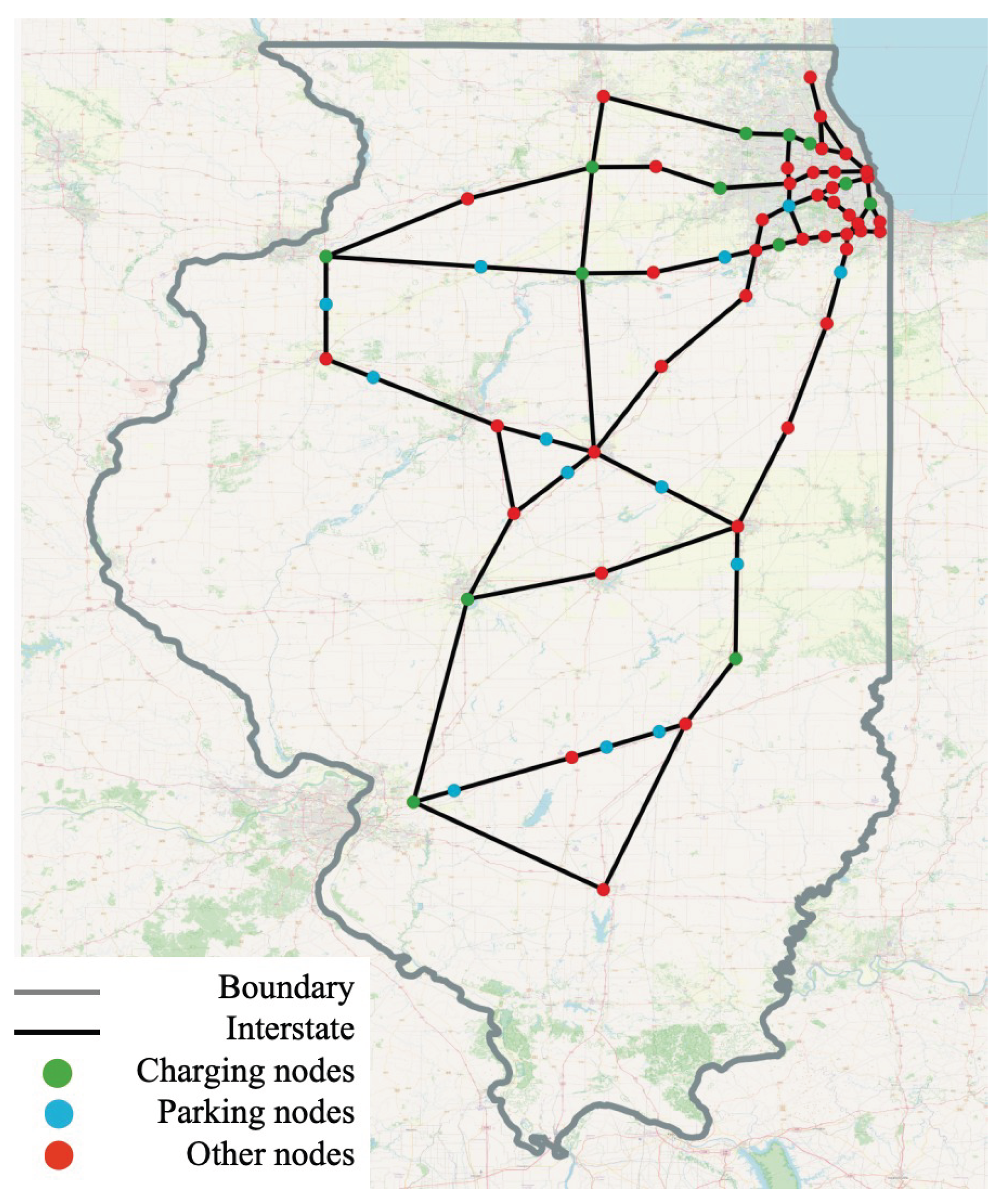
We conduct our numerical experiments on a simplified Illinois highway network as shown in Figure 1. The network consists of 66 nodes, including 13 designated parking nodes and 16 charging nodes, and 83 directed links. Among the charging nodes, 3 represent existing charging stations [42], while the remaining 13 are planned charging station according to Johnson and Brown (2023) [43]. The network primarily connects major cities within the state. Specifically, the network links nine major cities, namely, Chicago, Aurora, Joliet, Rockford, Springfield, Peoria, Elgin, Champaign, and Waukegan, which serve as origins and destinations for truck trips. Among these cities, all have populations exceeding 100,000, with the exception of Champaign [27]. Cities within the network are connected either by a single direct link or through a sequence of consecutive links.

5.2. Truck Time Windows

For each truck u, we specify its earliest departure time from its origin ${\sigma }_u$ and latest arrival time at its destination ${\kappa }_u$. ${\sigma }_u$ is randomly drawn from the time interval of 6:00–8:00 A.M. ${\kappa }_u$ is determined based on ${\sigma }_u$ and the minimum travel time ${\rho }_{o_u{d}_u}$ between the truck’s origin $o_u$ and destination $d_u$:

$${\kappa }_u={\sigma }_u+(1+\varphi ){\rho }_{o_u{d}_u}$$

(4)

where $\varphi$ is a parameter governing the degree of flexibility in the trucks’ time windows.

5.3. Other Parameters

The following parameters are adopted in this study. The fuel saving ratio for follower trucks in a platoon, denoted as ${\eta }_f$, is set to 16%, while the reduction rate for leading trucks, ${\eta }_l$, is set to 8% [28,44]. The average speed of trucks, $v_c$, is assumed to be 60 miles per hour [45]. Each truck is equipped with a battery capacity of 300 kWh, and charging rate, g, is set to 400 kW. The charging price, $p_c$, is considered to be $0.5 per kWh [46], and the driver wage rate, $p_d$, is set at $20 per hour [22]. The diesel fuel economy is 5 miles per gallon [47]. The diesel fuel price is assumed to be $5.5 per gallon, following the assumption used in Barua et al. (2023) [27]. Finally, the fuel efficiency of ETs are considered 1.5 kWh/mile based on the average fuel efficiency of state-of-the-art ET models Tesla Semi and Freightliner eCascadia [9]. The total operating hours for each truck is 10 h. The assumed battery capacity and consumption rate imply a nominal range of roughly 200 miles per full charge. The charging infrastructure is distributed such that feasible routes exist where the distance between consecutive charging opportunities remains within this range. In addition, the MILP formulation enforces energy feasibility via the SOC evolution and bounds (3b)–(3d); consequently, any route selected by the optimizer is energy-feasible by construction.

6. Results

In the results, we consider a baseline case consisting of 20 trucks where their origins and destinations are randomly generated along the Illinois highway among nine major cities in Illinois. The maximum platoon size is set to P = 5 for all experiments, unless stated otherwise. Similarly, the time window flexibility parameter is fixed at $\varphi =0.5$ throughout the analysis, unless specified otherwise. In addition, the proportion of ETs $\sigma$ is assumed to be 0.6 for the base case. All the numerical experiments are conducted on a MacBook Pro with an Apple M2 Pro chip, which has a 10-core CPU consisting of six performance cores and four efficiency cores and a 16-core GPU, 16 GB of RAM, and macOS Sonoma 14.5. The MILP instances are coded in Python 3.11 and solved using the default branch-and-cut framework (branch-and-bound combined with cutting planes and heuristics) of Gurobi Optimizer 11.0. All instances are solved to optimality within a time limit of 7200 s.

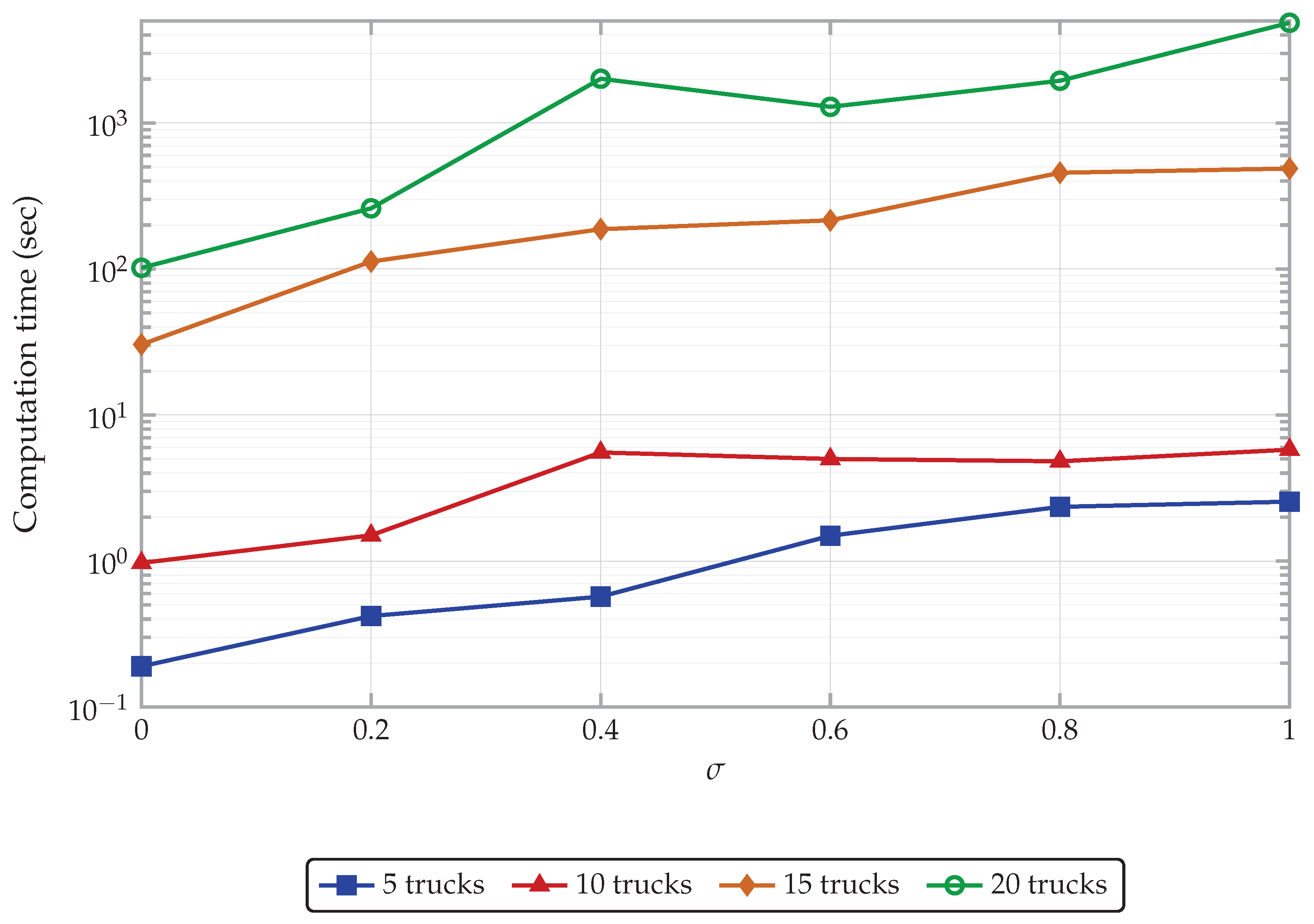
Figure 2 shows that the computation time increases with both fleet size and the proportion of ETs. The effect is especially pronounced for larger fleets, where the computation time rises rapidly as the ET proportion exceeds 0.4. These results highlight the greater computational complexity involved in optimizing a larger, more electrified fleet, underscoring the need for more efficient algorithms to support scalable platooning solutions.

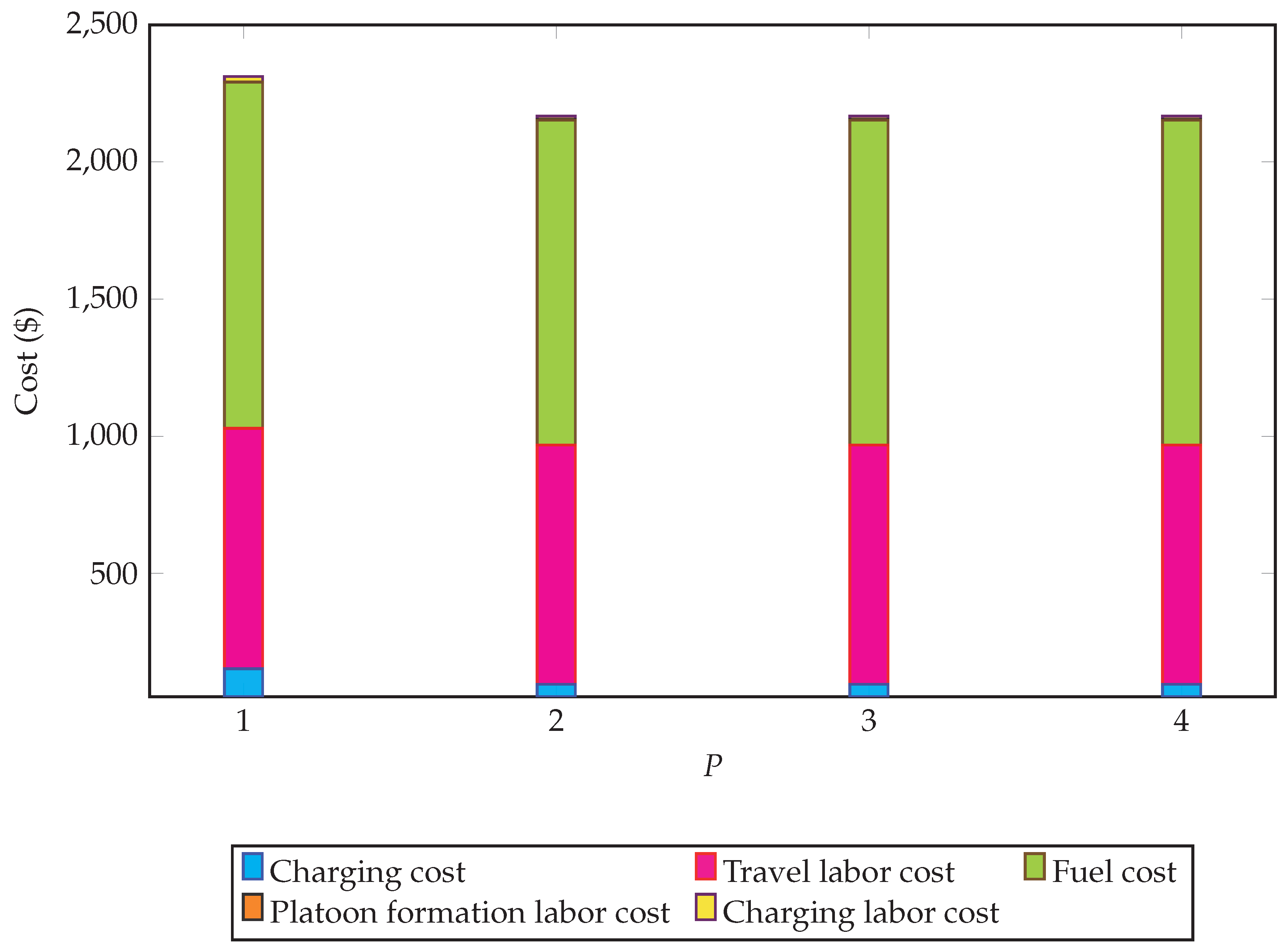
Figure 3 decomposes the total cost by component under different maximum platoon sizes. In this figure, fuel cost is consistently the largest portion in the total cost, followed by driver labor cost. In contrast, ET charging cost, platoon formation labor cost, and charging labor cost hold small shares in the total cost. Having a maximum platoon size of two results in a reduction in the total cost up—from $2312 to $2167—compared to without platooning. However, the total cost and the cost distribution remain largely unchanged when larger platoons are allowed. This indicates that, under the conditions examined in this study, increasing the maximum platoon size beyond two does not result in significant cost reductions. Therefore, we fix the maximum platoon size at two for the remainder of the analysis.

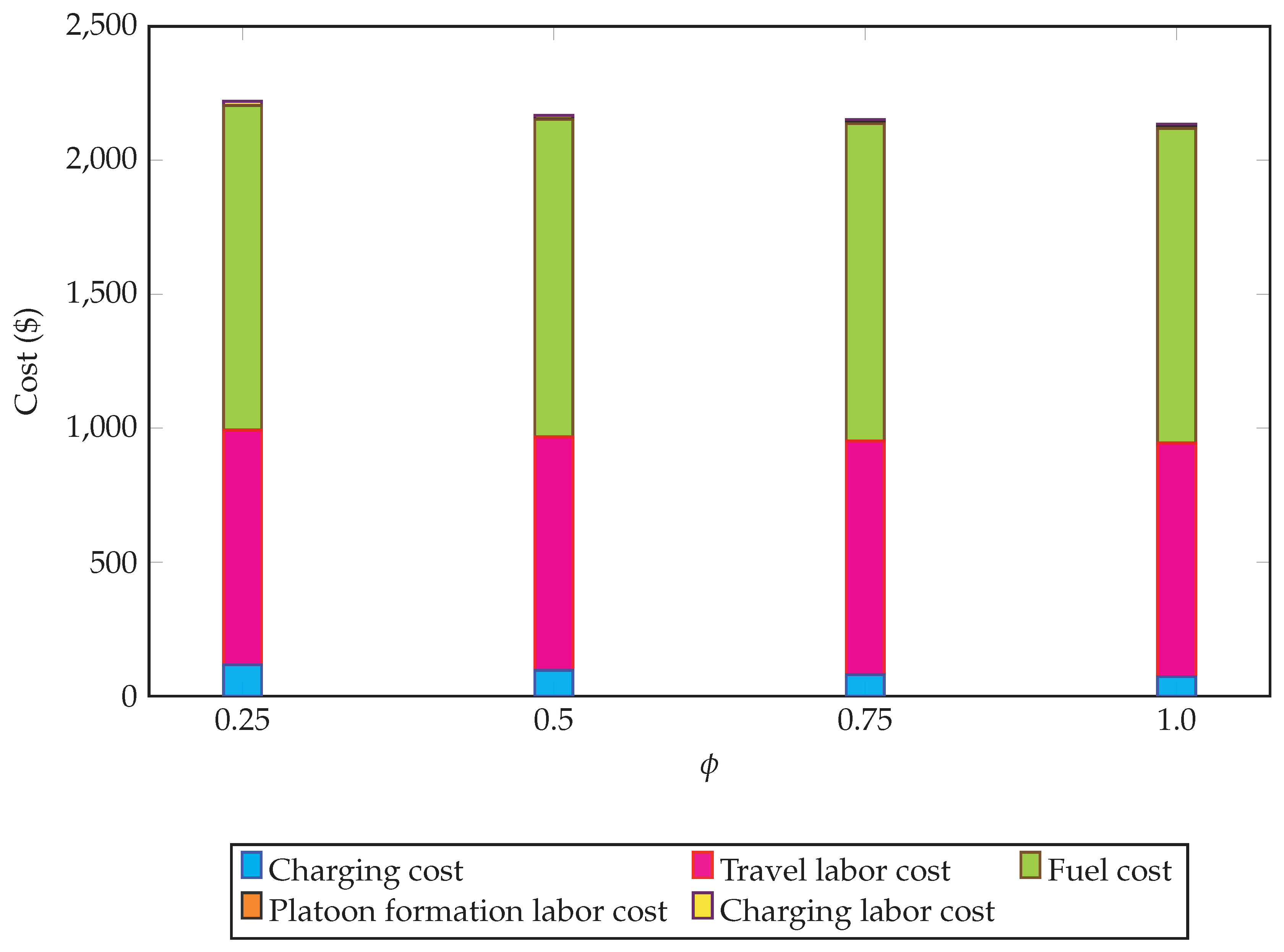
Figure 4 reports the total cost and its breakdown under different values of $\varphi$, which characterizes the flexibility of truck time windows. We find that the total cost decreases from $2220 to $2134 as $\varphi$ increases from 0.25 to 0.5. Afterward, the total cost and its breakdown remain almost constant. This initial reduction is primarily attributed to a decrease in fuel cost, indicating that when $\varphi$ increases from 0.25 to 0.5, trucks gain sufficient scheduling flexibility to fully exploit platooning opportunities, thereby achieving greater fuel savings. However, beyond $\varphi =0.5$, the additional scheduling flexibility does not lead to further reductions in fuel consumption.

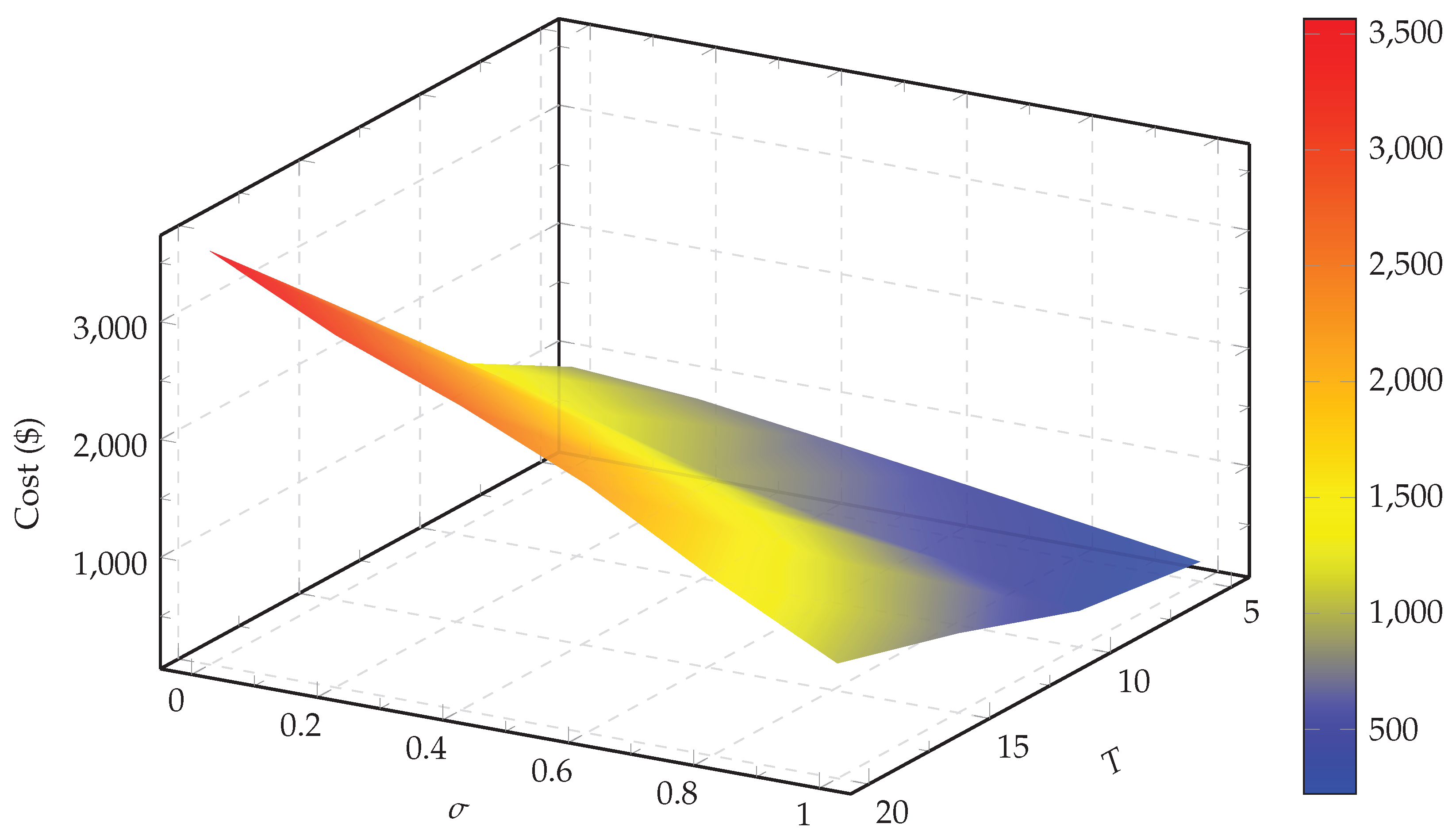
Figure 5 illustrates the impact of fleet composition on the total cost by varying both the number of trucks and the proportion of ET. As shown in the 3D surface plot, increasing the share of ETs consistently reduces the total cost, particularly when the fleet size is larger. The most substantial cost saving is observed when the proportion of ETs approaches 100%. Additionally, the total cost increases with the number of trucks, which is expected given that each truck contributes to the operational costs. This analysis underscores the substantial cost benefits of electrifying the truck fleet within platooning operations, particularly in cases involving a large number of vehicles.

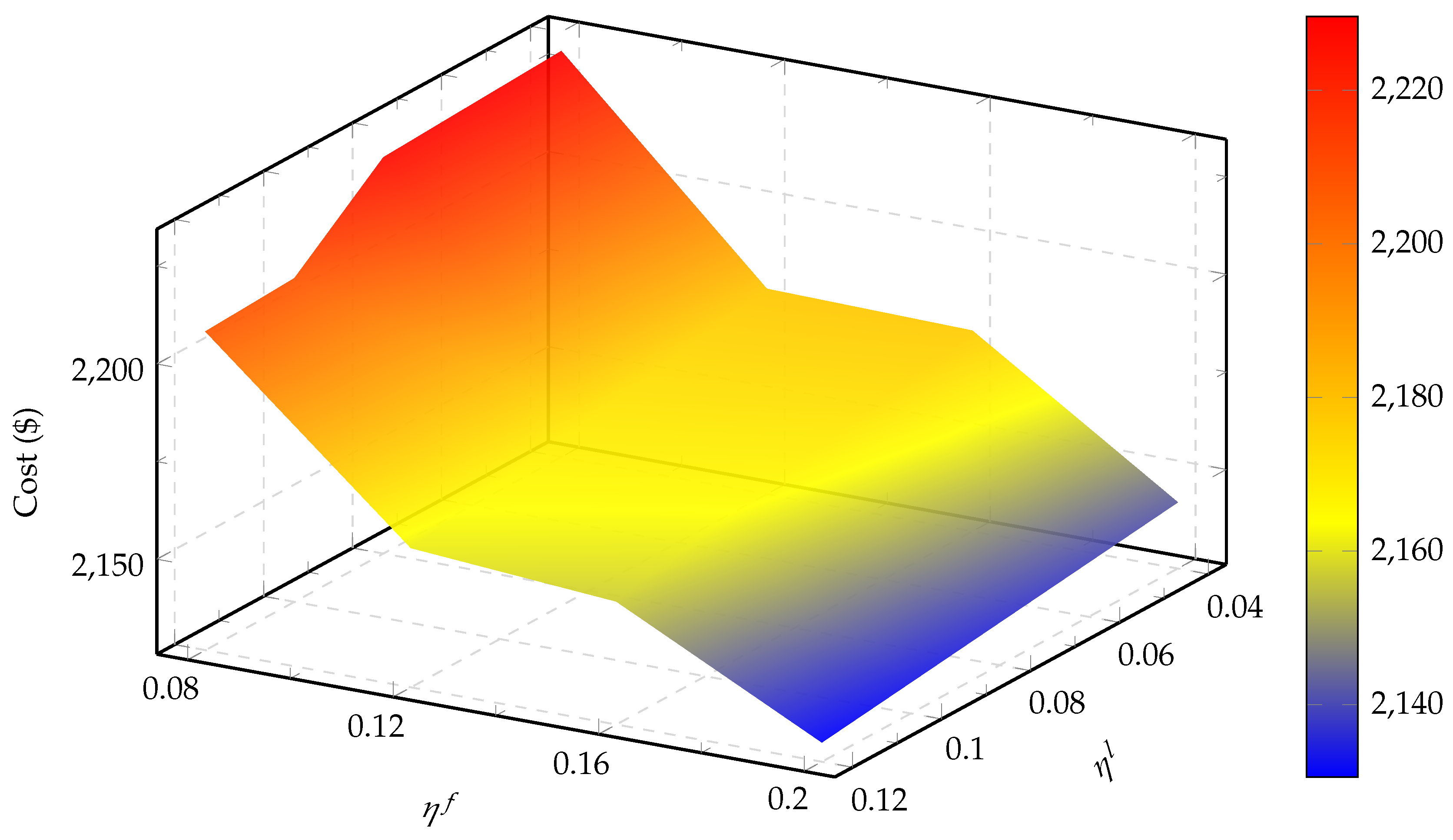
Figure 6 illustrates how total cost responds to changes in the fuel saving percentages by the leader and the follower trucks in a platoon. The surface plot demonstrates that as the follower fuel saving rate increases, the total cost systematically declines. A similar trend is observed with increasing leader fuel saving, although the effect is generally less pronounced than for followers. The lowest total costs are observed when both leader and follower fuel savings are maximized, shown by the blue region in the plot. These results emphasize that improvements in fuel efficiency—especially for follower vehicles, which make up the majority in platoons—can lead to substantial cost reductions.

To demonstrate the scalability of the proposed model formulation to larger problem sizes and to enable a comparison of operational settings, we conduct experiments under two scenarios, with platooning and without platooning, involving 60 trucks. To capture the inherent randomness in trucks’ time window, we generate five independent instances, each with 60 trucks. The results reported below represent the average performance across these five instances. 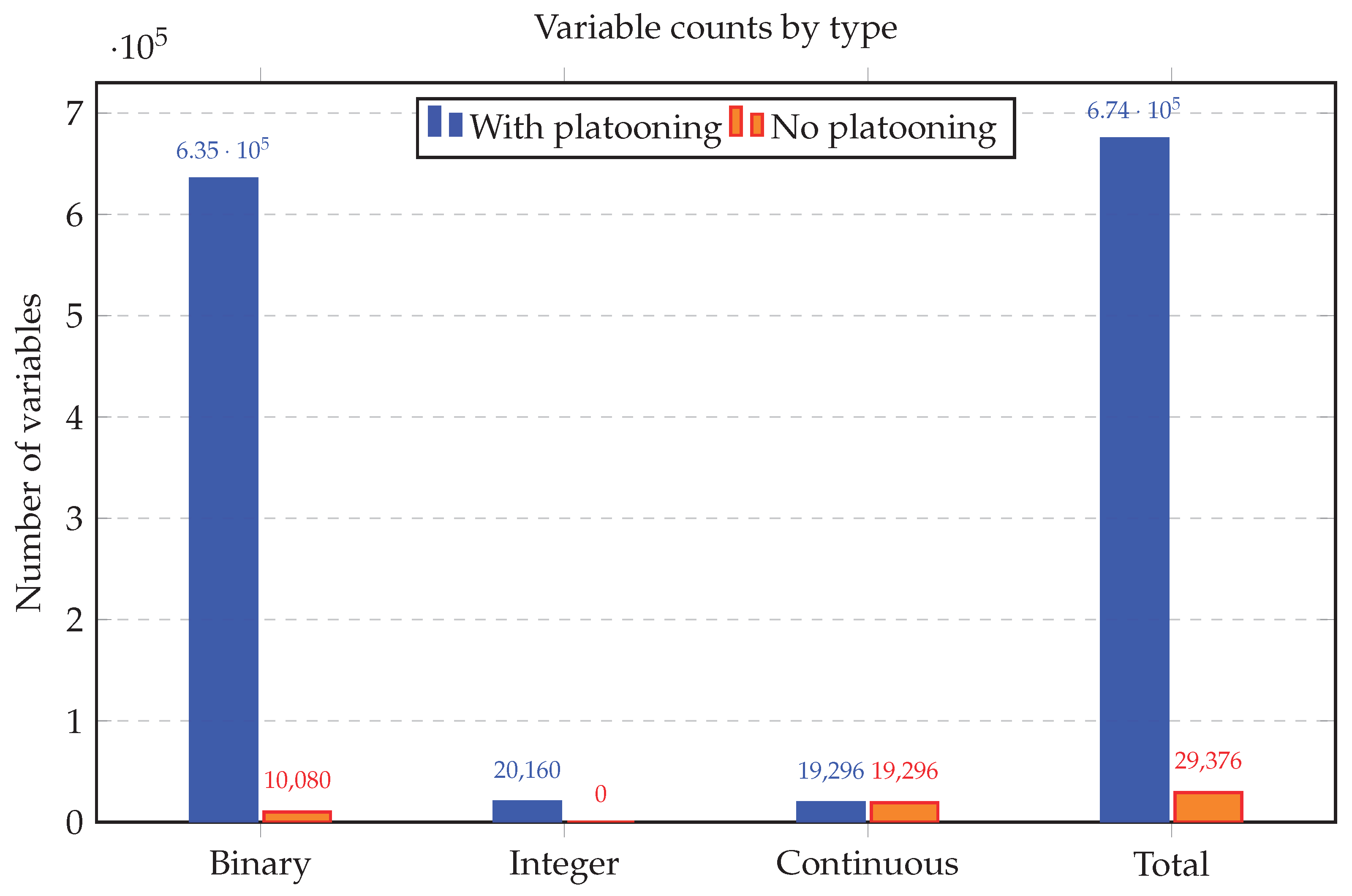Figure 7 highlights the significant modeling and computational impact of incorporating platooning decisions. The platooning formulation is substantially larger than the case without platooning, with the total number of variables increasing from 29,376 to 674,496, primarily due to the expansion of binary variables representing vehicle coordination decisions. While the number of continuous variables remains unchanged at 19,296, the added discrete structure greatly increases computational complexity. In addition to the number of variables, the number of constraints rises sharply from 51,648 to 3,126,048. As a result, the solution time rises from 20.37 s in the non-platooning scenario to 2532.41 s when platooning is enabled. From an economic perspective, however, the inclusion of platooning yields an improved objective value despite the much higher solution complexity. The total cost decreases from $5374 in the non-platooning configuration to $4964 with platooning, corresponding to a reduction of approximately $410 (7.6%). In addition, the model actively exploits platooning opportunities, generating 39.71 truck-hours of platooning and 2382.64 truck-miles of shared travel, whereas these quantities are naturally zero in the baseline case without platooning. Taken together, these findings indicate that platooning can provide measurable operational savings, but these benefits come at the expense of a significantly larger optimization model and a markedly longer solution time. Under the experimental settings considered in this study, a maximum platoon size of two captures most of the platooning benefits in the 60-truck experiments, while larger platoon sizes yield only marginal additional savings. This pattern is consistent with the 20-truck case. However, this finding depends on the specific network, fleet composition, and parameter settings considered here; under different operating conditions, larger platoons may offer greater benefits. A more comprehensive investigation of this aspect is left for future research.

7. Conclusions

This study addresses the integrated planning problem of routing, scheduling, and platooning for a mixed fleet of CTs and ETs, known as the MFTP problem. The model holistically incorporates charging scheduling, distinct operational constraints for both CTs and ETs, and the intricacies of platoon formation—including differential fuel savings for the leader and follower trucks in a platoon, the ET battery limits, charging station capacities, and platoon configuration. As such, the proposed MILP simultaneously optimizes the spatial–temporal coordination of trucks to form platoons, the routing and scheduling of trucks from multiple ODs, and the charging decisions of ETs.

We evaluate the model using extensive numerical experiments on a simplified Illinois interstate highway network. We find that allowing for platooning but limiting the platoon size to two trucks can already significantly reduce cost compared to traveling alone. However, allowing for longer platoons yields minimal additional savings. In addition, greater scheduling flexibility as reflected by larger truck time windows enables trucks to exploit more platooning opportunities, but only goes to a certain extent. A higher share of ETs further contributes to substantial cost reduction, particularly in larger fleets. Fuel cost remains the dominant cost component, underscoring the economic benefits of electrification and optimal platoon formation. We also include a no-platooning benchmark to provide a reference scenario. This comparison allows us to evaluate the marginal benefits of platoon coordination under identical operating conditions. Numerical results show that incorporating platooning reduces the total operational cost by 7.6% relative to the non-platooning scenario.

While the proposed model demonstrates strong potential for optimizing MFTP in real-world networks, the presented research can be extended in a few directions. First, the current approach will become computationally intensive to solve larger problem instances. Although this approach guarantees optimal solutions for the medium-sized instances tested, the computational burden may increase substantially for large-scale networks. Developing specialized solution algorithms, such as heuristic or decomposition-based approaches, could improve scalability and computational efficiency and represents an important direction for future research. Second, the model can be adapted into a stochastic framework to account for system uncertainties, especially those related to traffic, to enhance robustness of the solution. Third, this study assumes that all trucks are operated by drivers and does not consider automation. Exploring scenarios with autonomous ETs could be another promising research direction.