Article

Modeling the Mutual Enhancement of Regional Economy and Personal Quality of Life (QOL): A Case Study on the Mumbai–Ahmedabad High-Speed Rail Corridor in India

1
Department of Constructional Engineering, Graduate School of Engineering, Chubu University, Kasugai 487-8501, Japan
2
Center for Sustainable Development and Global Smart City, Chubu University, Kasugai 487-8501, Japan
3
Nippon Engineering Consultants Co., Ltd., Nagoya 451-0045, Japan
4
Department of Civil Engineering, Indian Institute of Technology Bombay, Powai, Mumbai 400-076, India
*
Author to whom correspondence should be addressed.
Future Transp. 2022, 2(4), 828-845; https://doi.org/10.3390/futuretransp2040046
Submission received: 5 August 2022 / Revised: 29 September 2022 / Accepted: 2 October 2022 / Published: 9 October 2022

Abstract

:
Among the various effects of high-speed rail (HSR), a direct benefit to users has been measured as an increase in the gross domestic product (GDP) by the conventional cost–benefit analysis (CBA), which was institutionalized in the U.K. In recent years, the importance of capturing indirect benefits to non-users has also been broadly discussed. The indirect benefits of HSR can mainly be classified into two perspectives: regional economy and personal quality of life (QOL). In this study, we modeled the mutual enhancement between those effects and analyzed the indirect benefits of the Mumbai–Ahmedabad high-speed rail (MAHSR), which is currently under construction as the first HSR in India, an emerging country with a rapidly growing economy. The indirect benefit to the regional economy along the MAHSR corridor was estimated by industry and by zone. Additionally, the indirect benefit on personal QOL by individuals’ attributes and by zone through the mutual enhancement with the regional economy was also estimated. The personal QOL tends to show greater effects in the middle cities than those in the two metropolitan areas of Mumbai and Ahmedabad. This method can evaluate interregional disparity by identifying the differences in benefits by person, according to age, income, etc., which cannot be evaluated based on a mass measure, e.g., GDP, in the conventional CBA.

1. Introduction

The Mumbai–Ahmedabad high-speed rail (MAHSR), India’s first high-speed rail (HSR), is currently under construction between Mumbai and Ahmedabad near the west coast of India, which is an emerging country with remarkable economic growth. This project is attracting attention as a milestone in the development of a nationwide HSR network in India. HSRs have been developed in many countries and regions, dating back to 1964, when the Tokaido Shinkansen of Japan was opened as the world’s first HSR. The Shinkansen brought about a paradigm shift in the flow of passengers for business and tourism in the 500 km-long metropolis between Tokyo, Nagoya, and Osaka, as well as remarkable economic development and changes in the social environment. The advantages of HSR as a mass means of passenger transportation over this distance are not only the economic benefits due to its speediness but also its environmental advantages in terms of energy efficiency compared to air travel and other modes of transportation [1], making it an effective contribution to sustainable development.
The MAHSR connects Mumbai and Ahmedabad, and its total length is about 500 km, which is almost the same as that of the Tokaido Shinkansen (Figure 1). Mumbai is the economic and financial center of India, as well as the capital city of Maharashtra, and Ahmedabad is the largest city in Gujarat. The journey time between Mumbai and Ahmedabad is about six hours by conventional train [2], while the fastest MAHSR train is planned to stop only at Surat and Vadodara and take about two hours [3]. The geographical arrangement of the metropolitan areas along the MAHSR—Mumbai, Surat, and Ahmedabad—is similar to that of Tokyo, Nagoya, and Osaka, and the total population of the districts (the administrative division under a state in India) is about 50 million [4] (Table 1). This is much higher than the approximately 30 million population in the Tokaido Shinkansen corridor region in 1960 [5], before the Shinkansen started its operation. The total construction cost of the MAHSR has been estimated as INR 0.98 trillion, and the total passenger demand has been forecasted as 166 thousand passengers per day in 2053 (JICA, 2014) [6].
The opening of a new transport infrastructure creates “facility operation effects” through improvement in accessibility to the other regions due to the reduction in travel time and costs. These spatial effects may have the potential to transform the interregional industrial structure; however, these effects have not been evaluated by conventional input-output (I/O) analyses. In this study, a combined model to simulate both I/O and spatial interactions was developed. Additionally, HSR improvement creates not only effects on the total GDP, which represents the effects on production by industries, but also differentiated effects on the level of happiness, or “quality of life (QOL)”, for individual citizens with different attributes such as income, age, and gender [8].
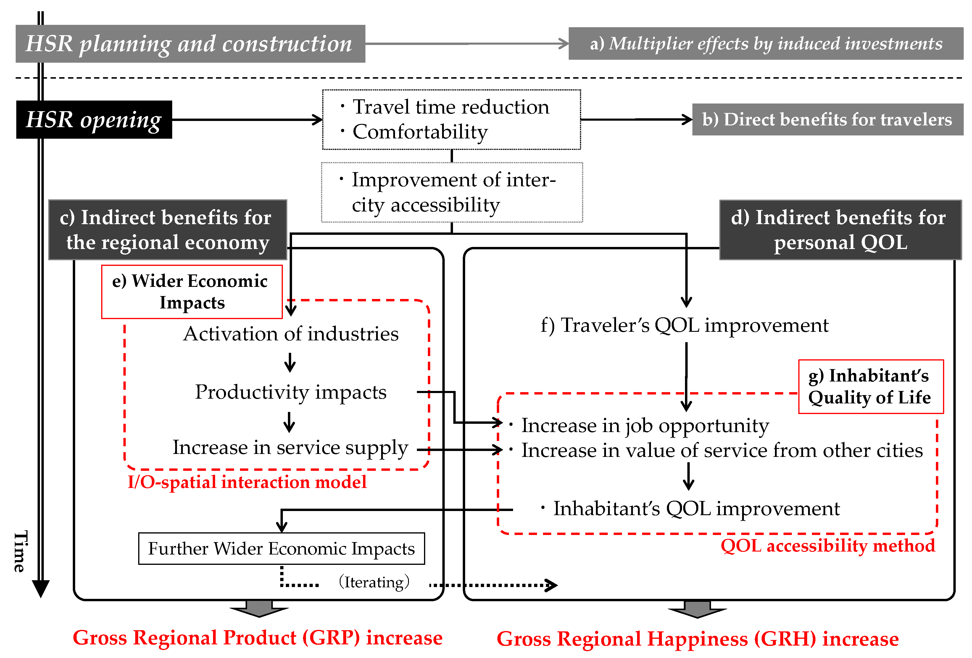
For the above reasons, this study developed a new structure of the model system illustrated in Figure 2. Along the time axis: (a) During the planning and construction phase of HSR, economic multiplier effects are generated in the short term by the construction of the HSR and its peripheral facilities, and by the investment and demand induced in related industries, which accompany the expectations for the opening of the HSR. (b) Subsequently, during the operation phase after the HSR opens, direct benefits for travelers will accrue as a result of reductions in time and improved comfort when traveling between cities along the HSR. On the other hand, the indirect benefits obtained by accessibility improvements between cities can mainly be classified into two perspectives, (c) regional economy and (d) personal QOL, which may contribute to an increase in the gross regional product (GRP) and gross regional happiness (GRH), respectively.
Indirect benefits for the regional economy include the stimulation of business-to-business communication and industry interaction, and medium- to long-term benefits, which are a part of the so-called (e) wider economic impacts [9], including productivity impacts and an increase in service supply. Indirect benefits for personal QOL include (f) the traveler’s QOL improvement in the short term, the subsequent increase in job opportunities, and the value of service from other cities, along with wider economic impacts, which will also (g) improve the QOL of inhabitant along the HSR corridor who do not use the HSR. This means that these effects are mutually enhanced, which is the main point of this study.
Afterward, this is expected to lead to further wider economic impacts, and the indirect benefits for the regional economy and the indirect benefits for QOL will be iterated.
In this study, applying the MAHSR corridor as a case study subject, the regional economic impacts were analyzed using the I/O–spatial interaction model (Section 3.1 and Section 4.1), and the inhabitant’s QOL improvement was analyzed using the QOL accessibility method (Section 3.2 and Section 4.2), along with the various indirect benefits associated with the accessibility improvements caused by the MAHSR. Then, the productivity impacts obtained by the I/O–spatial interaction model were incorporated into some of the QOL components, considering the mutual enhancement of these effects.

2. Literature Review

In the previous literature on HSR impacts, there has been much discussion on regional economies. For example, recently, Chen and Silva (2014) [10] analyzed the long-term impacts of the Spanish HSR network on employment and GDP, using a panel structural equation modeling (SEM) formulation. Li et al. (2016) [11] investigated the redistribution of economic activities in the Yangtze River Delta region in China by using a geographical network-weighted regression model and showed that the HSR drew the inflow to the second-tier cities along the HSR for investment activities. Vickerman (2015) [12] investigated the impact on the intermediate areas between major metropolitan areas along the network of northwest Europe and revealed that both levels of service and potential economic impacts are much less pronounced in these intermediate areas. Cheng et al. (2015) [13] examined changes in accessibility and provided evidence on changes in specialization for the main cities and their hinterlands in China and Europe, before concluding that the process of convergence and divergence differs at different stages of economic development. The abovementioned discussions are concluded in various ways depending on the social environment of each country or region, including population distribution, urban structure, geographical conditions, and economic stage. There is still much to be discussed before establishing an analytical method, and continued study and refinement are desirable.
In terms of accessibility through the passengers’ transportation, Yi and Kim (2018) [14] analyzed the spatial economic impacts of road and railway accessibility levels on manufacturing output in South Korea and revealed that there is a complementary—not a substitutive—relationship between the two transportation modes. In addition, changes in the accessibility of passenger flow by HSR will assist the development of a knowledge economy (Chen and Hall, 2012) [15] and regional innovation (Komikado et al., 2021) [16] in multiple cities; in other words, this will lead to communication effects related to the establishment of new businesses or the promotion of existing businesses. These effects have other characteristics than those caused by changes in freight transportation along with road construction. As for studies on accessibility and I/O–spatial interaction, Nakamura et al. (1983) [17] developed a model to predict industrial and commercial locations for a large metropolitan area in Japan, considering the economic distance between regions. Furthermore, Han et al. (2012) [18] examined the correlation between the industrial linkage and the actual changes in the number of employees in each industry before and after the opening of the Nagano Shinkansen in Japan, using a regression model that incorporates accessibility into the interdependence of inter-industry transactions and consumption demand obtained from the I/O table. These are examples of analysis based on Japan’s experience operating HSR (Shinkansen) systems over a long period of time, but there have been no previous examples of applications focused on new projects in countries and regions other than Japan.
Evaluation of benefit in the conventional cost–benefit analysis (CBA), which has been applied to many transportation projects, including HSR, targets the direct benefits to users. This concept has been recently reconsidered, and the importance of capturing indirect benefits to non-users such as wider economic impacts [9,19,20] or others (e.g., [21]) has also been broadly discussed. For example, the benefit in CBA considers the amount of output that would have been obtained as a benefit by allocating the extra time and cost obtained by travel time reductions to labor constructing railroads, roads, etc.; however, it only evaluates some of the benefits in the present age when transportation users’ purposes are diversified to different values, such as business, tourism, and medical care. In other words, it is more likely that the money is used to increase the level of happiness, or QOL, obtained from various values, such as leisure time and access to medical care. According to this approach, it is possible to evaluate the increase not in GDP as an economic effect, but in the QOL of individuals, i.e., the effect on humans, which can be more closely linked to the idea of “no one left behind”, which was outlined in the “SDGs” advocated by the United Nations (Hayashi et al., 2021) [22].
Based on the above, this study is novel in that it constructs and analyzes a more accurate integrated model linking the effects on the regional economy and the effects on personal QOL, using the HSR project in India, an emerging country with remarkable economic growth, as a case study.

3. Methodology and Data

3.1. I/O–Spatial Interaction Model

To represent the changes in the activity levels of industry and business induced by the shortening of the travel time between cities following the opening of the HSR, we constructed an I/O–spatial interaction model that additionally considers geospatial concepts in the I/O data. The modeling of geospatial distortions caused by the location of industries as an economic mass, which do not appear in general input–output data, was used to estimate the productivity impacts caused by the reduction in distance decay associated with the opening of the MAHSR. The authors developed the initial version of the I/O–spatial interaction model (Sugimori et al., 2021) [23] and applied an improved version (Sugimori et al., 2022) [24] in this research. The set of equations defined in the model is as follows:
D I N i j p q = A q p × P R O i p × P T i j q
D I N j q = i p D I N i j p q
where D I N i j p q is the demand for inter-industrial input from industry p in zone i to industry q in the surrounding zone j ; A q p is the input coefficient from industry q to industry p ; P R O i p is the production value of industry p in zone i ; and P T i j q is the probability of each industry in zone i trading with industry q in zone j . P T i j q is derived from Equation (3):
P T i j q = E M P L j q × ( G C i j ) λ q j E M P L j q × ( G C i j ) λ q
where E M P L j q is the number of employees (as an economic mass) of industry q in zone j , G C i j is the generalized travel cost from zone i to zone j , and λ q is the distance decay parameter of industry q . In this study, G C i j was calculated according to Equation (4) as the total monetary and time costs considering the transportation modal share.
G C i j = n s i j n · ( F i j n + ω · t i j n )
where s i j n , F i j n , and t i j n are the modal share, transport fare, and travel time, respectively, of transportation mode n from zone i to zone j , and ω is the time value.
The spatial distribution of demand (expenditure) is expressed by considering the probability of trade between industries, determined by the distance-decayed economic mass. Hence, we defined the main model as in Equation (5):
l n ( P R O j q ) = α q   l n ( D I N j q ) + c q
where α q is the scale parameter, differing for each industry q , and c q is a constant. This equation represents agglomeration effects in a similar form to the Cobb–Douglas production function. The details of this model are reported separately.

3.2. QOL Accessibility Method

3.2.1. Model Setting

The “QOL accessibility method” was formulated by Hayashi (2020) [25] as a project evaluation method that considers QOL. It is characterized by the fact that it evaluates the final attributed effect as a perceived value, varying by the attribute of each individual, which cannot be evaluated by the conventional CBA. The basic idea of this method is to quantitatively express the fact that the “accessible value” that a person living in a certain area enjoys from various facilities, such as commercial and medical facilities in the surrounding area, depends on their distance from such facilities, and the perceived value of such facilities depends on the attributes of each individual. This perceived value corresponds to QOL and, when aggregated for the entire population, it is possible to obtain a numerical value equivalent to gross national happiness (GNH), an indicator that has attracted attention since its adoption in Bhutan.
Several previous studies led to the establishment of this method. Hayashi and Sugiyama (2003) [8] divided the QOL indicators into five categories and evaluated the importance of de-suburbanization and social capitalization in urban planning in Japan, a country with a declining population. Kachi et al. (2007) [26] identified the planned retreat and re-concentration areas with an index for the social cost-effectiveness of QOL. Doi et al. (2008) [27] developed a QOL-based accessibility measure and a QOL performance measure based on a quantification of the weights of multiple elements of QOL. In addition, various case studies applying QOL analysis to urban planning were introduced, and the effects of QOL improvements caused by transportation infrastructure were quantitatively and visually demonstrated: for example, the case of Nanjing city in China by Gu et al. (2016) [28]. However, the study of Hayashi et al. (2004) [29] is the only example of a case study on the intercity passenger transportation system of HSR. This study applied the abovementioned method to estimate the inhabitants’ QOL in the MAHSR corridor following the opening of the MAHSR. The basic idea is as follows.
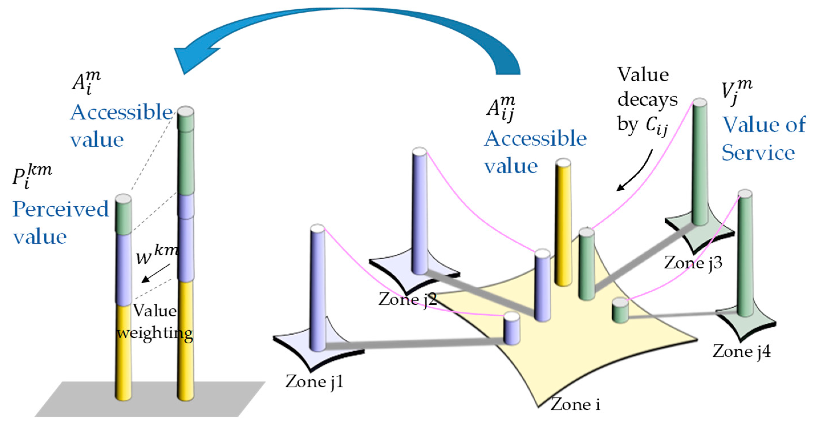
First, the degree to which a person living in zone i can access the value of a service provided by service m in the surrounding zone j, taking distance decay into account, is expressed in Equation (6):
A i m = j { V j m × e x p ( α m × C i j ) }
where A i m is the accessible value of service m from zone i, V j m is the value of service m in zone j, C i j is the time cost from zone i to zone j, and α m is the distance parameter for service m.
Next, the actual degree to which that accessible value is perceived depends on the weight of the value, which varies by person, as expressed in Equation (7):
P i k m = w k m × A i m
where P i k m is the perceived value of service m for person k in zone i, and w k m is the weight of the value of service m for person k. The concepts of Equations (6) and (7) are schematically illustrated in Figure 3. The figure shows that a person living in zone i can obtain the accessible value from various services in the surrounding zone j, which decays by spatial impedance and obtains the perceived value through the personal weight of the value.
Furthermore, the total perceived value that each person derives from the various services represents the QOL. If we aggregate the QOL by the population of the area, we obtain the value of the gross regional happiness (GRH). The above is shown in Equations (8) and (9):
Q O L i k = m P i k m
G R H = k i Q O L i k
where Q O L i k is the quality of life for person k in zone i.
This method is unique in that it measures the accessibility of the value of various services, such as shopping in shopping centers, the medical (hospital) service, and healing in green spaces, and allows for a uniform comparison of a wider variety of development effects in monetary terms that vary by individual.
The QOL factors (Table 2) in this study are categorized into five major components [8]: economic opportunity, living and cultural opportunity, amenity, safety and security, and environmental burden, and these are set as the type of service m. Furthermore, this analysis is unique in that the indicators related to the quality of travel (QOT) (Table 3) are detailed, considering the characteristics and advantages of HSR, which have been introduced for the first time in India. Regarding the factors related to service facilities, the generalized travel time required to access the facility is log-summed in proportion to the number of facilities, and the time reduction is considered to increase the accessible value (Equation (10)).
A i m = 1 α m l n j { V j m × e x p ( α m × C i j )   }
The travel time within a zone is regarded as one-half of the time needed to reach adjacent zones. The weights of QOT, estimated from the results of the questionnaire described below, are used to calculate the generalized travel time.

3.2.2. Data Used

Travel speeds, travel costs, etc., were set based on Open Street Map [7] as data on various facilities and rail and road networks that are necessary for QOL assessment. The general set-up conditions for transportation mode links are shown in Table 4. After the HSR opens, only HSR links will be added to the current network. Of these set-up conditions, the travel time and distance between HSR stations were based on the MAHSR’s Feasibility Study [6] (Table 5). In addition, the HSR fare was assumed to be approximately 1.5 times the current inter-city train (first-class air-conditioned car) fare on the existing rail.

3.2.3. Parameter Estimation

Various methods can be used to hypothetically obtain weights for multiple conditions and indicators related to QOL and QOT, such as the analytic hierarchy process (AHP) and the contingent valuation method (CVM). Among these methods, the conjoint analysis method is used to calculate the weight of the value, which is suitable for QOL analysis. Specifically, the “one-pair comparison method” is used, in which respondents select the profile they find more desirable from two profiles in which multiple conditions are combined in a survey. The results of the response yield the individual parameters using Equations (11) and (12) based on the binomial logit model:
P L i k = e x p ( β k m × A i m ) j e x p ( β k m × A j m )
β k m = β 0 k m + n β n k m
where P L i k is the probability of person k selecting (to live in) zone i, β k m is the parameter of person k for service m in zone j, and n is personal attributes (e.g., gender, age, income). The weight of value w k m in Equation (7) is derived from Equation (13): where β k c is the housing cost parameter.
w k m = β k m β k c

3.2.4. Questionnaire Survey

A questionnaire survey corresponding to the conjoint analysis, which is used to estimate the weight of the value for each attribute individually, was conducted in the major cities along the MAHSR—Mumbai, Surat, and Ahmedabad—through face-to-face interviews. The survey period was 2019, and as many samples as possible were collected for the survey duration, considering the balance of the number of samples for each individual. The sample size was 1142, and the composition ratios of the samples by individuals’ attributes are shown in Table 6. The sample ratios of male (70%) and young (63%) respondents are higher than those of the actual population. In addition, since the survey was conducted in the abovementioned big cities, probable biases on lifestyle and educational level are to be noted.
The survey items mainly consisted of individuals’ attributes, current values regarding QOL indicators, pairwise comparisons regarding QOL indicators, and pairwise comparisons regarding QOT indicators. An example of pairwise comparisons for QOL indicators is shown in Figure 4. Specifically, the questions were structured so that the respondents chose the preferred one from two sites with different combinations of multiple indicator conditions. Since the conditions for the living environment are expected to differ depending on the current residential site, the questions were set to ask about the percentage (%) change from the current environment. Similarly, in the case of QOT, the questions were structured so that the respondents chose the preferred one from two transportation options with different conditions.

4. Results of Analysis and Interpretations

4.1. Results of I/O–Spatial Interaction Model

4.1.1. Estimated Parameter

Table 7 shows the results of the parameter estimation through regression analysis using Equation (5) of the I/O–spatial interaction model. For industries and services with a relatively high scale parameter α value (infrastructure services, hotels and restaurants, public services, etc.), the increase in demand for input can be inferred to be likely to spill over multiplicatively to a higher output. In other words, it can be expected that those industries and services have a stronger relationship with the passengers’ accessibility. In addition, since the primary industry is located depending on land use conditions, the R2 value of agriculture, forestry, and fishery is significantly low.

4.1.2. Estimated Productivity Impacts

Productivity impacts were calculated by inputting the change in inter-zonal distance decay by the time reduction associated with the MAHSR opening into the I/O–spatial interaction model. The resulting annual GRP increase by zone is shown in Figure 5a, averaging 1.8% for all zones. The breakdown of the data is shown in Figure 5b for the “commerce” example and in Figure 5c for the “other services” (medical, education, finance, etc.) example. GRP increased in all zones for all industries (Figure 5a) but some areas decreased GRP due to the straw effect. This means that, if zone A has higher attractiveness than other zones after the HSR opening, zone A will become more competitive in the multi-regional transactions and gain more shares than before. Otherwise, zone A will lose competitiveness and shares.

4.2. Mutual Enhancement of Regional Economy and Personal QOL

4.2.1. Estimated Parameter of QOL and QOT by QOL Accessibility Method

Table 8 and Table 9 show the parameters of each QOL and QOT indicator for each individual’s attributes, respectively, obtained by the parameter estimation using the QOL accessibility method. Relative comparison values among attributes are listed here, using “male, 35–49 years old, middle income” as the reference value. For example, the parameter of “female, 35–49 years old, middle income” for job opportunities is 1.44 (=1.11 + 0.33), which means females are expected to see job opportunities as important (more than males). Similarly, Table 8 shows that the weight of the value for travel time to each facility differs depending on the attributes. Table 9 shows that the people with a low income see the travel cost as important more than the people with a high income, which means the income gain will increase the value of time. Note that only parameters with p-values less than 0.2 are used and listed in these tables.

4.2.2. Mapping with Personal QOL Impacts

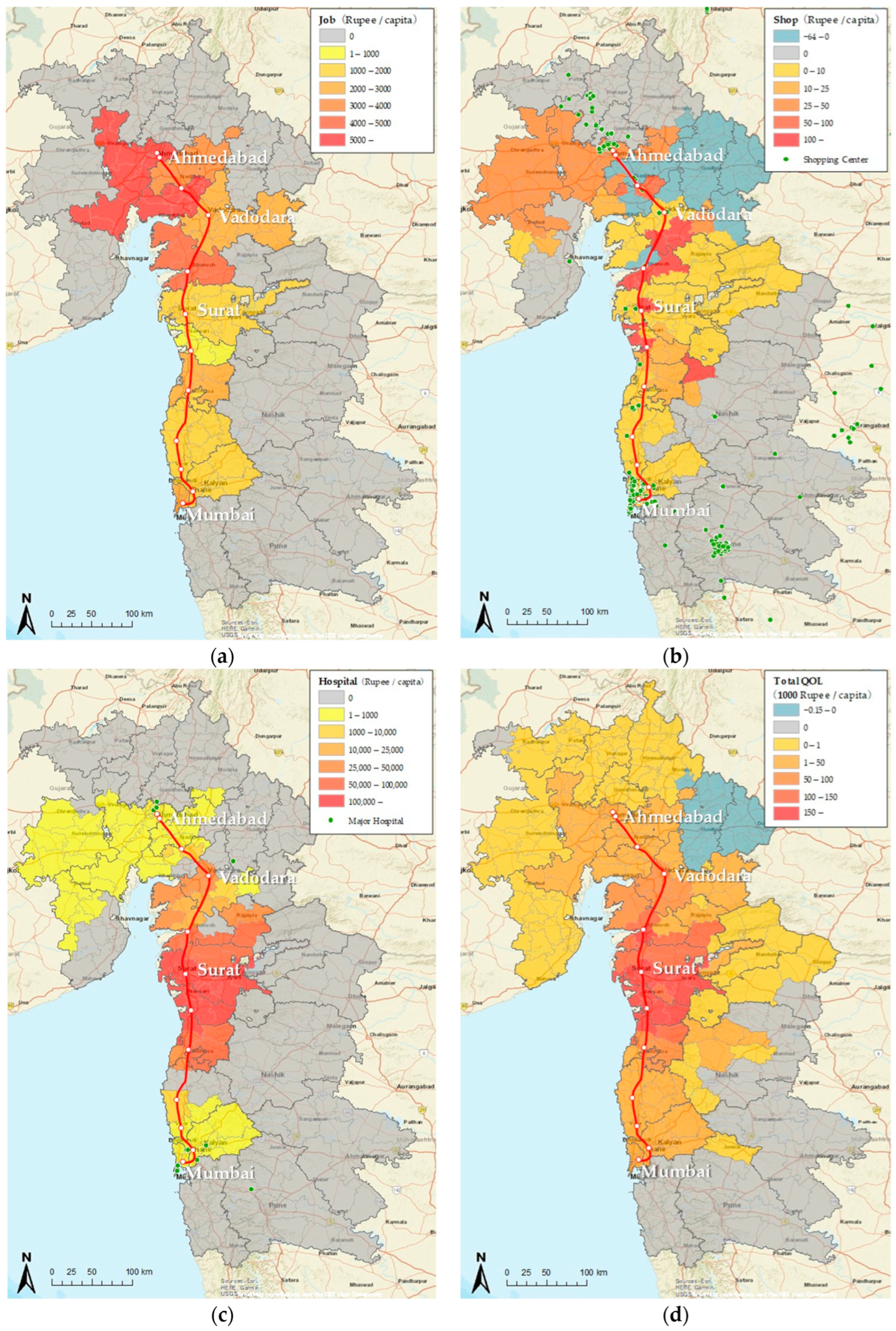
The geographic distribution of personal QOL impacts associated “with the MAHSR” was visualized by mapping, and Figure 6a–d show job opportunities, travel time to shopping centers, travel time to major hospitals, and total QOL, respectively. The QOL impacts were calculated by comparing the accessibility “without the MAHSR” and “with the MAHSR”. In order to consider the mutual enhancement of the regional economy and personal QOL, the GRP increase in Figure 5a was incorporated as the job opportunity increase. Similarly, the GRP increase in “commerce” in Figure 5b was incorporated as the increase in the number of shopping centers, and the GRP increase in “other services” in Figure 5c was incorporated as the increase in the number of major hospitals.
Comparing the results, it was found that the distribution trends of the increase in personal QOL were different in each zone, due to the different changes in the accessibility of each zone after the opening of the MAHSR, depending on the location of various facilities. Specifically, Figure 6a shows that the improvement in personal QOL by job opportunity increase is the greatest in the vicinity of the large city (Ahmedabad). This indicates that the mutual enhancement—as the industrial development associated with the HSR leads to a higher income and, in turn, personal QOL improvement—is remarkable in these cities. On the other hand, Figure 6b–d shows that, when various QOL factors are taken into account, personal QOL tends to show greater effects in the middle cities rather than in the two metropolitan areas of Mumbai and Ahmedabad, where various types of facilities are originally accessible within each area. This suggests that the MAHSR will bring broad spillover QOL impacts throughout the corridor region, where accessibility to metropolitan areas is newly improved. As described above, it is now possible to represent the geographical distribution of various QOL impacts, which vary according to the type of value perceived by the individuals.

4.2.3. QOL Impacts by Personal Attributes

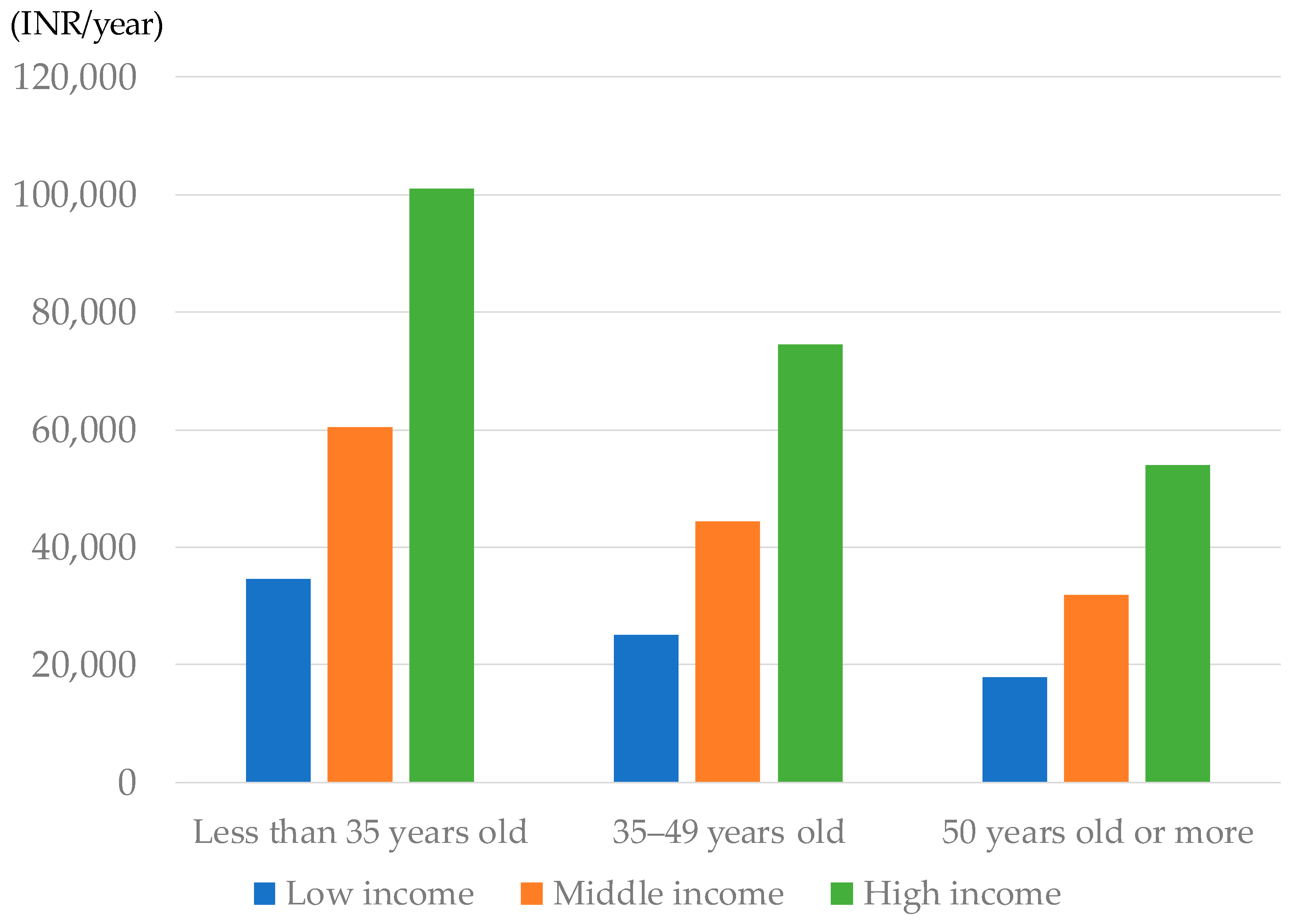
Table 10 and Figure 7 show the results of the total personal QOL increase after the MAHSR opening, averaged by population by attribute in the MAHSR corridor. Overall, the annual increase in GRH, which is the total QOL, was estimated at 2.8%. Due to data availability limitations, the following assumptions were made regarding population by income class. The population’s multidimensional poverty [30] by the district was deducted, considering the HSR users’ characteristics. The population was then allocated using India’s overall income class ratios, i.e., low income: 40%, middle income: 50%; and high income: 10% [31].
Figure 7 shows that younger persons tend to experience a greater QOL increase than older persons. In addition, for all age classes, persons with a higher income have a greater QOL increase. This may be attributed to the higher time value of trips for any purpose, for persons in a higher income class. The result shows that the increase in the regional product affects individual income growth, which consequently enhances inhabitants’ QOL, as illustrated in Figure 2. Especially in India, with a fast-growing economy, personal income is increasing, which further changes the sense of values and lifestyles to enhance the impacts of high-speed rail. This implies that the QOL brought about by the improved accessibility associated with the MAHSR opening is expected to become more pronounced.
As described above, it is now possible to analyze the effects of HSR by region and by individuals’ attributes, considering the mutual enhancement of the regional economy and personal QOL, and to conduct a more detailed policy analysis of transportation projects.

5. Conclusions and Discussion

In this study, we modeled the mutual enhancement of regional economy and personal QOL and analyzed the indirect benefits of the Mumbai–Ahmedabad high-speed rail (MAHSR), which is currently under construction as the first high-speed rail (HSR) in India, an emerging country with a rapidly growing economy. The regional economic impacts as indirect benefits were analyzed using the I/O–spatial interaction model, and the inhabitants’ QOL improvements were analyzed using the QOL accessibility method, among the various indirect benefits brought by the MAHSR. Thus, the productivity impacts obtained by the I/O–spatial interaction model were incorporated into a part of the QOL components, considering the mutual enhancement of those effects.
The indirect benefit for the regional economy along the MAHSR corridor was estimated by industry and by zone. In addition, the indirect benefit for personal QOL by individuals’ attributes and by the zone through the mutual enhancement with the regional economy, was also estimated. The detailed QOL impacts show that personal QOL improvements in job opportunities are greatest in the vicinity of the large city (Ahmedabad). This indicates that the mutual enhancement—the industrial development associated with the HSR leading to a higher income and, in turn, personal QOL improvements—is remarkable in these cities. On the other hand, the personal QOL when various QOL factors are considered tends to show greater effects in the middle cities than those in the two metropolitan areas of Mumbai and Ahmedabad. This means that the MAHSR has broad spillover QOL impacts throughout the corridor region where accessibility is improved.
As described above, this method can evaluate interregional disparity by identifying the differences in benefits (by person) according to age, income, etc., which cannot be evaluated based on a mass measure, e.g., gross domestic product (GDP), in the conventional CBA. Additionally, QOL is totally different from various wider economic impacts, which were mainly discussed in Europe, in that it analyzes the impacts in a fully aggregated manner dedicated to an individual person. This makes it possible for it to be used for evaluation from the viewpoint of inclusiveness in the SDGs, and to be utilized to aid in various future policy evaluations in a society with diverse values. In further research, it will be desirable to refine the questionnaire survey methodology and value estimation method by obtaining a wider range of statistical data and to apply/demonstrate the methodology in multiple cases in other HSR corridors in India and abroad.

Author Contributions

Conceptualization, Y.H.; methodology, Y.H. and S.S.; software, T.T.; validation, S.S.; formal analysis, S.S. and T.T.; investigation, K.V.K.R.; resources, T.T. and H.M.; data curation, T.T.; writing—original draft preparation, S.S.; writing—review and editing, Y.H. and H.T.; visualization, T.T.; supervision, T.I. All authors have read and agreed to the published version of the manuscript.

Funding

This research received no external funding.

Institutional Review Board Statement

Not applicable.

Informed Consent Statement

Not applicable.

Data Availability Statement

The data presented in this study are available upon request from the corresponding author.

Conflicts of Interest

The authors declare no conflict of interest.

References

  1. Rothengatter, W.; Hayashi, Y.; Fujisaki, K.; Kato, H.; Okuda, T.; Shibahara, N. Climate change impacts of intercity transport in the context of external costs and their internalisation. In Intercity Transport and Climate Change: Strategies for Reducing the Carbon Footprint, 2015th ed.; Hayashi, Y., Morichi, S., Oum, T.H., Rothengatter, W., Eds.; Springer: Cham, Switzerland, 2014; pp. 89–175. [Google Scholar]
  2. Indian Railways, Indian Railways Enquiry. Available online: http://www.indianrail.gov.in/enquiry/StaticPages/StaticEnquiry.jsp?StaticPage=index.html&locale=en (accessed on 31 July 2022).
  3. MAHSR Operational Plan. Available online: https://www.nhsrcl.in/en/project/mahsr-project-operational-planss (accessed on 31 July 2022).
  4. Ministry of Home Affairs, Government of India, Census Tables, D-01. Available online: https://censusindia.gov.in/census.website/data/census-tables (accessed on 31 July 2022).
  5. Statistics Bureau of Japan, 1960 Population Census, Population, Area and Population Density for Shi, Ku, Machi and Mura: 1960. Available online: https://www.e-stat.go.jp/en/stat-search/files?page=1&layout=datalist&toukei=00200521&tstat=000001036867&cycle=0&tclass1=000001037497&tclass2val=0 (accessed on 31 July 2022).
  6. Japan International Cooperation Agency (JICA), Ministry of Railways, Republic of India (MOR), Joint Feasibility Study for Mumbai-Ahmedabad High Speed Railway Corridor, Final Report. July 2015. Available online: https://www.nhsrcl.in/en/project/feasibility-study-report (accessed on 31 July 2022).
  7. Source: OpenStreetMap. Available online: https://www.openstreetmap.org (accessed on 31 July 2022).
  8. Hayashi, Y.; Sugiyama, I. Dual strategies for the environmental and financial goals of sustainable cities: De-suburbanization and social capitalization. Built Environ. 2003, 29, 8–15. [Google Scholar] [CrossRef]
  9. Department for Transport, Transport Analysis Guidance (TAG) Unit A2-1 Wider Economic Impacts Appraisal. May 2019. Available online: https://www.gov.uk/guidance/transport-analysis-guidance-tag#overview (accessed on 31 July 2022).
  10. Chen, G.; Silva, J.A. Estimating the provincial economic impacts of high-speed rail in Spain: An application of structural equation modelling. Procedia-Soc. Behav. Sci. 2014, 111, 157–165. [Google Scholar] [CrossRef] [Green Version]
  11. Li, X.; Huang, B.; Li, R.; Zhang, Y. Exploring the impact of high speed railways on the spatial redistribution of economic activities-Yangtze River Delta urban agglomeration as a case study. J. Transp. Geogr. 2016, 57, 194–206. [Google Scholar] [CrossRef]
  12. Vickerman, R. High-speed rail and regional development: The case of intermediate stations. J. Transp. Geogr. 2015, 42, 157–165. [Google Scholar] [CrossRef]
  13. Cheng, Y.; Loo, B.P.Y.; Vickerman, R. High-speed rail networks, economic integration and regional specialisation in China and Europe. Travel Behav. Soc. 2015, 2, 1–14. [Google Scholar] [CrossRef] [Green Version]
  14. Yi, Y.; Kim, E. Spatial economic impact of road and railroad accessibility on manufacturing output: Inter-modal relationship between road and railroad. J. Transp. Geogr. 2018, 66, 144–153. [Google Scholar] [CrossRef]
  15. Chen, C.; Hall, P. The wider spatial-economic impacts of high-speed trains: A comparative case study of Manchester and Lille sub-regions. J. Transp. Geogr. 2012, 24, 89–110. [Google Scholar] [CrossRef]
  16. Komikado, H.; Morikawa, S.; Bhatt, A.; Kato, H. High-speed rail, inter-regional accessibility, and regional innovation: Evidence from Japan. Technol. Forecast. Soc. Chang. 2021, 167, 120697. [Google Scholar] [CrossRef]
  17. Nakamura, H.; Hayashi, Y.; Miyamoto, K. A land use-transport model for metropolitan areas. Pap. Reg. Sci. Assoc. 1983, 51, 43–63. [Google Scholar]
  18. Han, J.; Hayashi, Y.; Jia, P.; Yuan, Q. Economic Effect of High-Speed Rail: Empirical Analysis of Shinkansen’s Impact on Industrial Location. J. Transp. Eng. 2012, 138, 1551–1557. [Google Scholar] [CrossRef]
  19. Graham, D.J.; Gibbons, S. Quantifying wider economic impacts of agglomeration for transport appraisal: Existing evidence and future directions. Econ. Transp. 2019, 19, 100121. [Google Scholar] [CrossRef]
  20. Chèze, C.; Nègre, R. Wider economic impacts of high-speed rail: Example of agglomeration benefits assessment on Bretagne Pays de Loire high speed rail project. Transport. Res. Procedia 2017, 25, 5307–5324. [Google Scholar] [CrossRef]
  21. Silvestri, B.; Rinaldi, A.; Roccotelli, M.; Fanti, M.P. Innovative Baseline Estimation Methodology for Key Performance Indicators in the Electro-Mobility Sector. In Proceedings of the 6th International Conference on Control, Decision and Information Technologies (CoDIT), Paris, France, 23–26 April 2019; pp. 1367–1372. [Google Scholar]
  22. Hayashi, Y.; Morita, H.; Takeshita, H.; Kachi, N.; Kato, H. (Eds.) Mainstreaming Quality of Life in Evaluation of Transport and Spatial Planning, 1st ed.; Akashi Shoten: Tokyo, Japan, 2021; 380p. (In Japanese) [Google Scholar]
  23. Sugimori, S.; Hayashi, Y.; Takeshita, H. Empirical analysis on industrial sectors for quality of life improvement along high-speed rail corridors. In Frontiers in High-Speed Rail Development, 1st ed.; Hayashi, Y., Rothengatter, W., Seetha Ram, K.E., Eds.; Asian Development Bank Institute: Tokyo, Japan, 2021; pp. 218–228. [Google Scholar]
  24. Sugimori, S.; Hayashi, Y.; Takeshita, H.; Isobe, T. Evaluating the Regional Economic Impacts of High-Speed Rail and Interregional Disparity: A Combined Model of I/O and Spatial Interaction. Sustainability 2022, 14, 11545. [Google Scholar] [CrossRef]
  25. Hayashi, Y. QOL Accessibility Method for Project Evaluation. Expressway Automob. 2020, 63, 6–10. (In Japanese) [Google Scholar]
  26. Kachi, N.; Kato, H.; Hayashi, Y. A computable model for optimizing residential relocation based on quality of life and social cost in built-up areas. J. East. Asia Soc. Transport. Stud. 2007, 7, 1460–1474. [Google Scholar]
  27. Doi, K.; Kii, M.; Nakanishi, H. An integrated evaluation method of accessibility, quality of life, and social interaction. Environ. Plan. B 2008, 35, 1098–1116. [Google Scholar] [CrossRef]
  28. Gu, F.; Hayashi, Y.; Shi, F.; Zhang, H.; Kato, H. Measuring and mapping the spatial distribution of the quality of life in a city: A case study in Nanjing. Int. J. Urban Sci. 2016, 20, 107–128. [Google Scholar] [CrossRef]
  29. Hayashi, Y.; Doi, K.; Sugiyama, I. Evaluating infrastructure projects by means of measures of the quality of life. Proc. JSCE 2004, 751, 55–70. (In Japanese) [Google Scholar] [CrossRef]
  30. MPI Results for Districts in India. Available online: https://ophi.org.uk/wp-content/uploads/Table-5a-India-District-MPI-2018-1.xlsx (accessed on 31 July 2022).
  31. India Style. Available online: https://warp.da.ndl.go.jp/info:ndljp/pid/11066444/www.jetro.go.jp/ext_images/_Reports/02/2018/fe2e7bc10241316e/7_all.pdf (accessed on 31 July 2022).
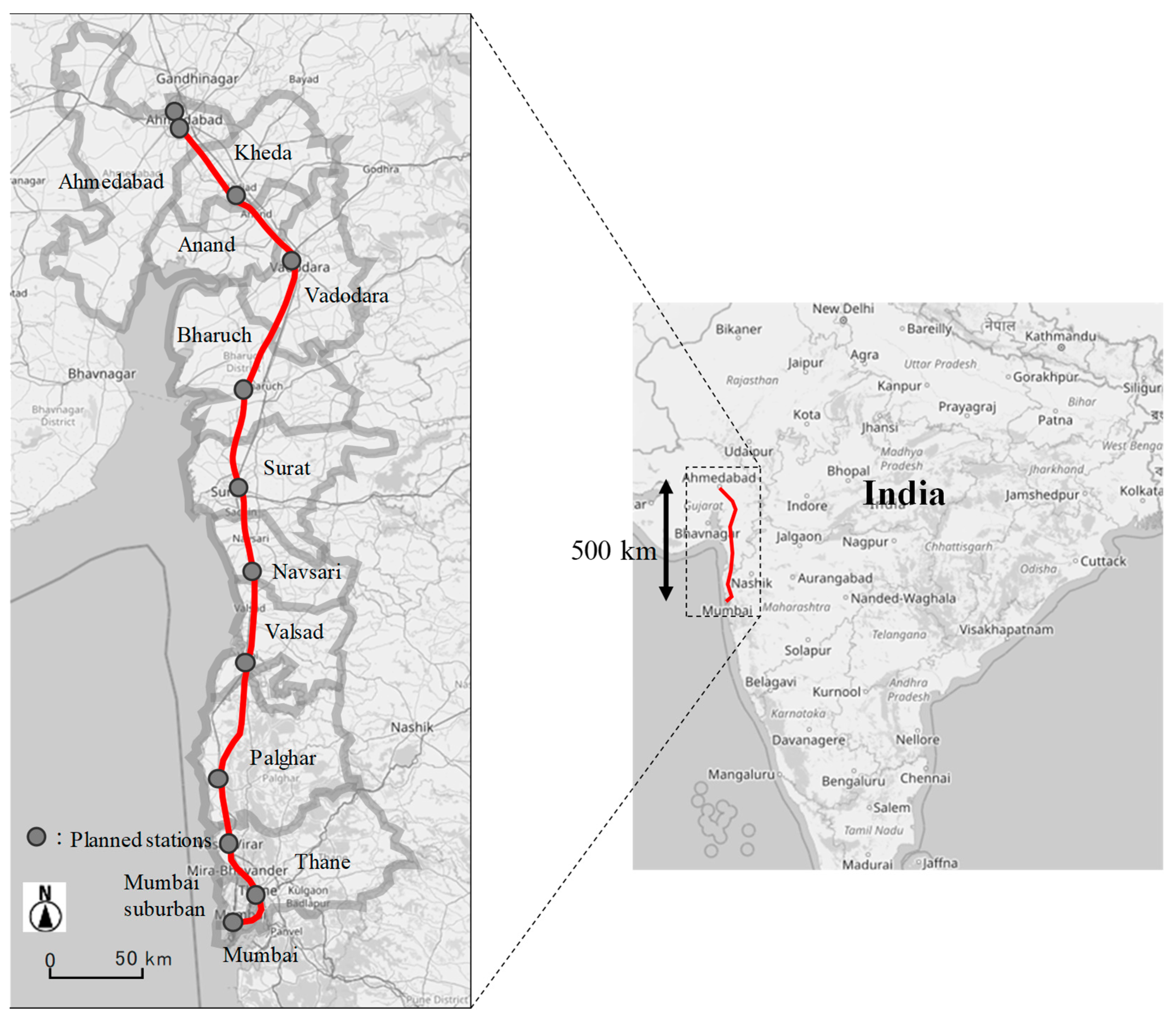
Figure 1. The MAHSR route map (under construction) [7].
Futuretransp 02 00046 g001
Figure 2. Mechanism and model system of HSR benefits.
Futuretransp 02 00046 g002
Figure 3. The model of the QOL accessibility method.
Futuretransp 02 00046 g003
Figure 4. An example of the questionnaire on pairwise comparisons.
Futuretransp 02 00046 g004
Figure 5. Estimated increase in annual GRP by zone: (a) all industries and services; (b) commerce; (c) other services.
Futuretransp 02 00046 g005
Figure 6. Estimated QOL impacts distribution in the MAHSR corridor by: (a) job opportunities; (b) travel time to shopping centers; (c) travel time to major hospitals; (d) total QOL (sources: the authors visualized the results based on Esri, HERE, Garmin, USGS, Intermap, INCREMENT P, NRCan, Esri Japan, METI, Esri China (Hong Kong), Esri Korea, Esri (Thailand), NGCC, © OpenStreetMap contributors, and the GIS User Community).
Futuretransp 02 00046 g006
Figure 7. Averaged personal QOL increased by age and income class.
Futuretransp 02 00046 g007
Table 1. Overview of the districts along the MAHSR corridor [4].
StateDistrictPopulationArea (km2)Population Density (per km2)
GujaratAhmedabad7,214,2258107890
Kheda2,299,8853953582
Anand2,092,7453204653
Vadodara4,165,6267546552
Bharuch1,551,0196509238
Surat6,081,32245491337
Navsari1,329,6722246592
Valsad1,705,6783008567
MaharashtraThane (including Palghar)11,060,14895581157
Mumbai (including suburban)12,442,37360320,634
Total49,942,69349,2831013 (average)
Table 2. Quality of life (QOL) factors.
CategoryFactorsIndicators
Economic opportunityAccess to officeCommuting time (min)
Job opportunityJob opportunities (%)
ResidenceHousing cost (INR)
Living and cultural opportunityMedical careTravel time to major hospitals (min)
Educational opportunityTravel time to college/university (min)
TourismTravel time to tourist locations (min)
Shopping opportunityTravel time to shopping centers (min)
Recreational opportunityTravel time to entertainment facilities (min)
Travel time to cultural places (min)
Travel time to sporting facilities (min)
AmenityComfort of livingFloor space (sq. ft.)
CleanlinessCleanliness (level)
GreennessGreenery (%)
Safety and securitySafe neighborhoodCrime rate (dummy)
Road safetyTraffic accidents (dummy)
Disaster riskFlood risk (dummy)
Environmental burdenAir pollutionAir quality (AQI)
Noise pollutionNoise level (dB)
Water qualityDrinking water quality (level)
Table 3. Quality of travel (QOT) indicators.
IndicatorsDetail
Total travel cost (INR)The cost to travel from the origin to the destination
Total travel time (min)The time need to travel from the origin to the destination
Delays in scheduled time (min)How many minutes for which the journey is delayed
Prior booking time for seat reservation (days)How many days before the journey should tickets be booked
Air conditioning (A/C) (dummy)Whether air conditioning is available
Freedom while traveling (dummy)Ability to work, read books, eat, etc., during the journey
Number of transfersThe number of transfers required from the origin to the destination
Wi-Fi (dummy)Whether Wi-Fi is available
Table 4. General conditions of transportation mode links (source: authors).
Link TypeSpeed (km/h)Fare (INR/km)
MAHSR(Derived from Table 5)5
Rail (Intercity)503.5
Rail (Express)502
Rail (Local)250.25
Metro352
Expressway502
Road250.8
Table 5. Train operation plan for the MAHSR [6].
StationDistance from the Origin (km)Travel Time (min)
FastestLocal
Mumbai0.00:000:00
Thane28.0-0:10
Virar65.2-0:24
Boisar104.2-0:39
Vapi167.9-0:59
Bilimora216.6-1:15
Surat264.60:581:32
Bharuch323.1-1:52
Vadodara397.11:322:14
Anand/Nadiad447.4-2:32
Ahmedabad500.21:592:50
Sabarmati505.82:072:58
Table 6. Composition ratios of the samples by individuals’ attributes.
ItemCategoryRatio
GenderMale70%
Female30%
AgeYoung (Less than 35 years old)63%
Middle (35–49 years old)21%
Old (50 years old or more)16%
IncomeLow (Less than INR 25,000/month)36%
Middle (INR 25,000–100,000/month)47%
High (INR 100,000/month or more)17%
Table 7. Estimated parameters by I/O–spatial interaction model.
α c R2
Agriculture, forestry, and fishery0.9880.1440.53
(3.34)(0.04)
Manufacturing (including mining)0.9590.6340.99
(35.01)(1.63)
Construction0.9760.2900.97
(16.71)(0.39)
Infrastructure services1.031−0.5360.94
(11.42)(-0.46)
Commerce0.9570.5480.97
(15.69)(0.71)
Hotels and restaurants1.077−1.1910.92
(10.48)(−1.04)
Other services0.9710.3490.95
(12.85)(0.35)
Public services1.186−2.6110.91
(9.29)(−1.90)
Note: the bracketed values are t-values.
Table 8. Estimated parameters of quality of life (QOL) indicators.
IndicatorsConst.FemaleYoung (Less Than 35 Years Old)Old (50 Years Old or More)Low Income (Less Than INR 25,000/Month)High Income (INR 100,000/Month or More)
Commuting time1.00 ***−0.31 **
Job opportunities1.11 ***0.33 **−0.63 ***
Housing cost0.84 ***
Travel time to major hospitals1.74 ***0.34 *−0.40 **0.30
Travel time to college/university0.73 ***0.21
Travel time to tourist locations0.140.27 *
Travel time to shopping centers0.34 ***
Travel time to entertainment facilities0.54 ***0.25 *−0.22 *
Travel time to cultural places0.75 ***
Travel time to sporting facilities0.67 ***−0.23 *
Floor space0.60 ***−0.47 **
Cleanliness0.81 ***-0.17
Greenery0.43 **0.29 *0.33−0.31 **
Crime rate2.60 ***−0.39 *−0.47 **
Traffic accidents0.70 ***0.49 *
Flood risk0.56 ***−0.55 *
Air quality1.26 ***−0.31 *−0.23−0.18
Noise level0.84 ***−0.36 *
Drinking water quality0.51 ***0.22
Significance codes: *** p < 0.001, ** p < 0.01, * p < 0.05. ρ2 = 0.40.
Table 9. Estimated parameters of quality of travel (QOT) indicators.
IndicatorsConst.FemaleYoung (Less Than 35 Years Old)Old (50 Years Old or More)Low Income (Less Than INR 25,000/Month)High Income (INR 100,000/Month or More)
Total travel cost (INR)0.0014 ***−0.0003 ***−0.0002 **0.0005 ***−0.0005 ***
Total travel time (min)0.0050 ***−0.0007 **−0.0008 **
Delay in scheduled time (min)0.0153 ***−0.0046 *−0.0030
Prior booking time for the seat reservation (days)0.0954 ***
Air conditioning (A/C) (dummy)0.6628 ***−0.2472 *−0.3509 ***0.4259 ***
Freedom while traveling (dummy)0.7357 ***-0.1369−0.2702 *
Number of transfers (dummy)0.4408 ***−0.1665 ***0.1359 *
Wi-Fi (dummy)0.5232 ***−0.2596 **−0.2290
Significance codes: *** p < 0.001, ** p < 0.01, * p < 0.05. ρ2 = 0.26.
Table 10. Summary of estimated QOL impacts by personal attributes.
AgeIncome ClassQOL Increase (INR Million/Year)PopulationAveraged Personal QOL Increase (INR/Year)
MaleYoung (less than 35)Low77,3612,186,54335,380
Middle169,8852,733,18062,157
High56,954546,638104,190
Middle (35–49)Low38,7261,522,51125,436
Middle86,5851,903,12845,496
High29,313380,62377,012
Old (50 or more)Low19,7981,126,47617,575
Middle44,5271,408,10131,622
High15,092281,61953,590
FemaleYoung (less than 35)Low63,1331,875,98233,653
Middle137,2602,344,98258,534
High45,698468,99697,438
Middle (35–49)Low33,3311,360,35224,502
Middle73,3771,700,43743,152
High24,318340,08471,506
Old (50 or more)Low19,9821,100,22618,162
Middle44,4081,375,28632,290
High14,968275,05854,419
Publisher’s Note: MDPI stays neutral with regard to jurisdictional claims in published maps and institutional affiliations.