2. Literature Review
Ramp meters have been employed in many urban locations in the United States and around the world as a means of mitigating congestion caused by growing demand [
1,
2,
3,
4,
5,
6,
7,
8,
9,
10]. By controlling the flow of traffic onto freeways—particularly around peak usage times—ramp meters allow freeways to operate at a higher volume while lowering the likelihood or severity of decreases in level of service. Additional observed benefits of ramp metering include decreases in crash rates, lower emissions, and reduced fuel consumption [
1].
Over the past several years, multiple studies have been conducted that confirm the benefits of ramp metering. For example, in the Minneapolis–St. Paul region in Minnesota, a study comparing traffic operations with and without ramp metering showed that average travel speeds on the freeway increased from 23 miles per hour (mph) to 39 mph during peak travel times when the local freeway on-ramps were metered compared to no metering. In addition, overall travel delay decreased by over 20 percent in the study corridor [
11]. On the Monash freeway in Melbourne, Australia, the implementation of ramp metering increased traffic flow by 4.7 percent and average speed by 24.5 percent during the morning peak hour; while during the afternoon peak hour, traffic flow increased by 8.4 percent and average speed by 58.6 percent [
12].
Several approaches may be taken to implement a ramp metering program depending on transportation needs and the goals of the transportation agency. Meters are generally classified into two different types: pre-timed and traffic responsive. Pre-timed ramp meters are based on historical data, whereas traffic-responsive meters use real-time data to detect and react quickly to changing traffic conditions. Controls may be implemented at a local level based only on conditions immediately surrounding the ramp or on a systemwide level based on conditions of a freeway corridor including multiple on-ramps [
1,
4].
Pre-timed metering at both the local and systemwide level is determined based on historical data, making it simpler to implement than traffic-responsive metering. When congestion problems are predictable, pre-timed meters can generally meet needs for managing flow onto the freeway. However, pre-timed metering rates must be regularly monitored and periodically updated to accommodate changes in traffic patterns, which may result in additional long-term expenses. Furthermore, pre-timed meters cannot adjust to traffic conditions in real time, which may employ rates that are either too restrictive or too free for the actual conditions [
1,
6].
Traffic-responsive metering depends on real-time data collection. This often makes initial programming for the meters more difficult but reduces the number of required updates long-term once the meters have been tuned in the field. Local traffic-responsive metering can be used to mitigate congestion based on data collected on the freeway near the ramp. These meters rely on data collected via sensors to determine an acceptable rate at which vehicles can be released onto the freeway from a specific on-ramp. Systemwide traffic-responsive metering coordinates metering rates across the entire freeway section to effectively manage entry onto the freeway for optimal use [
1,
6].
Although ramp metering has proven to considerably improve freeway service, it also has some drawbacks. Ramp meters tend to favor those who commute longer distances on the freeway, as the time spent waiting on the on-ramp is more than made up for by the travel time saved on the freeway. Those who travel shorter distances may not benefit or may even be negatively affected by wait times at on-ramps, which may exceed time savings on the freeway. If queueing on the ramp is not properly managed, ramp metering can have negative effects on the larger road network. While freeway travel times may improve, ramp delay may become too high, and in some cases spillback onto arterial roads can lead to serious disruptions [
3]. Public acceptance of ramp metering is valuable to its overall success; excessive wait times or slow metering rates may lead drivers to ignore the meters or lobby for other methods of traffic management [
1].
Several algorithms are available for the setting of ramp metering rates. Though not discussed in detail in this paper, these approaches generally use a combination of local and systemwide traffic-responsive metering rates to optimize traffic flow during peak periods. Most algorithms seek to find a balance between achieving optimal traffic flow on the freeway system while preventing the queue along the on-ramp from causing spillback onto the local street network [
12,
13,
14,
15,
16,
17,
18].
The overall performance of ramp metering algorithms is typically measured by assessing various conditions of freeway performance. While there are many performances measures that pertain to the freeway such as capacity, volume to capacity (v/c) ratio, level of service, and travel time, there are few that directly evaluate freeway
ramp performance [
1]. Additionally, research has been completed to estimate queue length and wait time at typical unsignalized and signalized intersections as well as at tollways. Much of the research done to assess queue length and wait time at those locations uses traffic queue theory, time-dependent models, and simulation data [
19,
20]. It is also recognized that the field of artificial intelligence and advanced optimization has been growing significantly in recent years, with applications including but not limited to online learning, scheduling, transportation, medicine, data classification, and ramp metering [
21,
22,
23,
24,
25,
26]. As the field of artificial intelligence continues to evolve, its application to traffic data analysis has become more prevalent. It is known that some research has been completed to date with respect to neural network algorithms and their applicability to optimizing traffic flow along a corridor with ramp metering [
21]. These sources provide valuable information, similarities, and possibilities as they pertain to ramp metering, but they are not discussed thoroughly in this study based on the overall objectives of the research. These may be explored for future research.
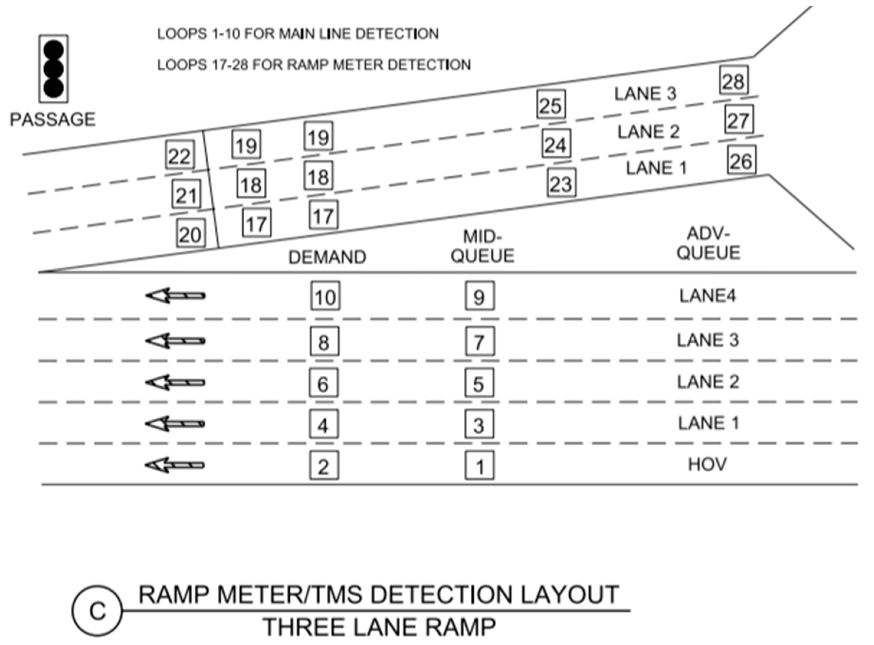
Occupancy and traffic volume data are often gathered by loop detectors along an on-ramp. As shown in
Figure 1, several sets of detectors are used in freeway ramp operations. Detectors 20 through 22 represent the passage queue detection (PQ), detectors 23 through 25 represent the intermediate queue detection (IQ), while detectors 26 through 28 represent the excessive queue detection (EQ) [
27]. Although loop detectors are useful mechanisms that provide essential traffic data to transportation agencies, loop detection is known to be imperfect, may experience malfunctions, and the quality of the detector data can deteriorate over time [
28,
29]. Causes of loop detection failure and data quality deterioration can stem from multiple sources, which can include pavement cracking and movement, breakdown of wire insulation, poor sealants, inadequate splices and electrical connections, damage caused by construction, electronics unit failure, and electrical surges [
28]. Data quality difficulties can also stem from vehicles passing over two detectors simultaneously as they change travel lanes, vehicles may be missed altogether, poor traffic lane pavement markings, traffic composition, and changes in traffic density [
9,
29].
Using the loop detector data, several ramp queue length estimation algorithms have been developed and analyzed, including a conservation model, a Kalman filter, and the Highway Capacity Manual (HCM) back of queue method [
3,
7,
8,
9]. For this research, the HCM back-of-queue method proved to be ineffective, as it substantially underestimated actual queue lengths, thus it will not be discussed in detail in this paper [
9]. However, some variations of the conservation model and Kalman filter equation have been developed, which will be discussed in this section.
The conservation model for estimating queue length has been used for several decades but appears to have been first applied directly to metered on-ramps by Vigos et al. in 2006 [
7]. The conservation equation developed in that research (with some minor naming modifications for clarity) is shown in Equation (1):
where:
= number of on-ramp queued vehicles in the current period (veh)
= number of on-ramp queued vehicles in the previous time period (veh)
= time period (min)
= number of vehicles entering the on-ramp during a given time period (veh/min)
= number of vehicles exiting the ramp during a given time period (veh/min).
Equation (1) has since been used to predict queue length in several other research studies [
3,
8,
9]. The original equation developed for the conservation model in Equation (1) required the volume entering and exiting the ramp to be equal, but errors were found in the detector-estimated volumes when compared with field recorded traffic volumes [
9]. Many difficulties are introduced when relying solely on the detector data, particularly, as mentioned previously, that vehicles can be double-counted or missed altogether [
9]. Because of this potential for error, the original conservation model equation was modified to balance the volumes entering and exiting the ramp which is shown by a volume-balancing ratio
C in Equation (2) [
9]:
where:
By using this volume-balancing ratio, it is presumed the conservation model will produce more accurate queue length estimates. The volume-balancing ratio has been calculated by balancing the counts in 15 min periods [
3] or by setting it as a constant value calculated in real time [
8,
9]. Prior to incorporating this volume-balancing ratio in Equation (1) it was discovered that the correlation between the estimated queue length and the time occupancy was only 0.63 [
8]. The relationship between volume data from the detector and the estimated number of vehicles was also found to be nonlinear, as the results gave a correlation coefficient of merely 0.18 between the two variables [
8]. Therefore, it is likely that there are other factors outside the capability of this equation that affect queue length such as detector error, driver distraction, poor weather, and traffic incidents. However, in analyzing 20 data sets from ramp meters in Milwaukee, Wisconsin, it was found that the volume-balancing ratio improved the conservation model considerably in nearly every case. Therefore, it appears that the use of the volume-balancing ratio will improve the reliability of queue length estimates [
8].
The Kalman filter model has also been used for estimating queue length at on-ramps [
3,
7,
8,
9]. A Kalman filter is an algorithm that can combine multiple data measurements to produce more accurate estimates. In the case of traffic flow, the conservation model presented in Equation (2) is enhanced by the addition of occupancy data and ramp characteristics as inputs that are also used to predict queue length as shown in Equation (3):
where:
= Kalman filtering constant (generally 0 < < 1)
= number of on-ramp queued vehicles calculated from detector time occupancy data (veh)
is calculated as outlined in Equation (4):
= time occupancy collected by loop detectors (%)
= length of the on-ramp (ft)
= number of lanes
= effective vehicle length, (vehicle length + safety distance between vehicles) (ft).
With the inclusion of detector occupancy and ramp characteristics, such as the length of the on-ramp, the number of lanes, and the vehicle length, the Kalman filter algorithm uses these known measurements to estimate unknown parameters—the ramp queue length in this case—with greater accuracy. The Kalman filter constant
can update during each minute to account for “noise” in the data from the detectors. The Kalman filter equation can further be improved by the inclusion of the volume-balancing ratio
C in Equation (5) [
9]:
By using the volume-balancing ratio, as occurred with the conservation model, the queue length estimates obtained by Wu et al. [
9] improved significantly in nearly all cases, and in only a select few cases were slightly more errors introduced. These errors were found to occur in the Kalman filter models because when the volume-balancing ratio is close to 1 (the detector volume entering and exiting the ramp are nearly equal), the Kalman filter coefficient
is also close to zero, but the equation still adds queue length to the estimate from the coefficient
which would introduce additional error. In contrast, when the volume-balancing ratio is not close to 1, the Kalman filter equation yields more reliable results than the conservation model. Overall, both the Kalman filter and conservation model, especially when using the volume-balancing ratio, provide generally accurate estimates of the actual queue length [
9].
However, none of the research done previously proposes a simple and reliable method that can be used to estimate ramp meter queue length in real time. Initial ramp queue length estimation research relied solely on microscopic simulation to produce the Kalman filter algorithm [
7], and later research suggested that the traffic engineering community has no reliable methodology to predict the on-ramp vehicle queue length [
8]. In addition, no research has been found to date that attempts to predict ramp meter
wait time in real time. All existing methods found during this research in relation to ramp meter wait times have simply been completed through visually observing ramp wait times or have required ongoing data collection and calibration on a ramp-by-ramp basis to estimate wait times [
11,
30]. This research will propose a method to estimate ramp meter wait times without ongoing data collection.
4. Data Collection
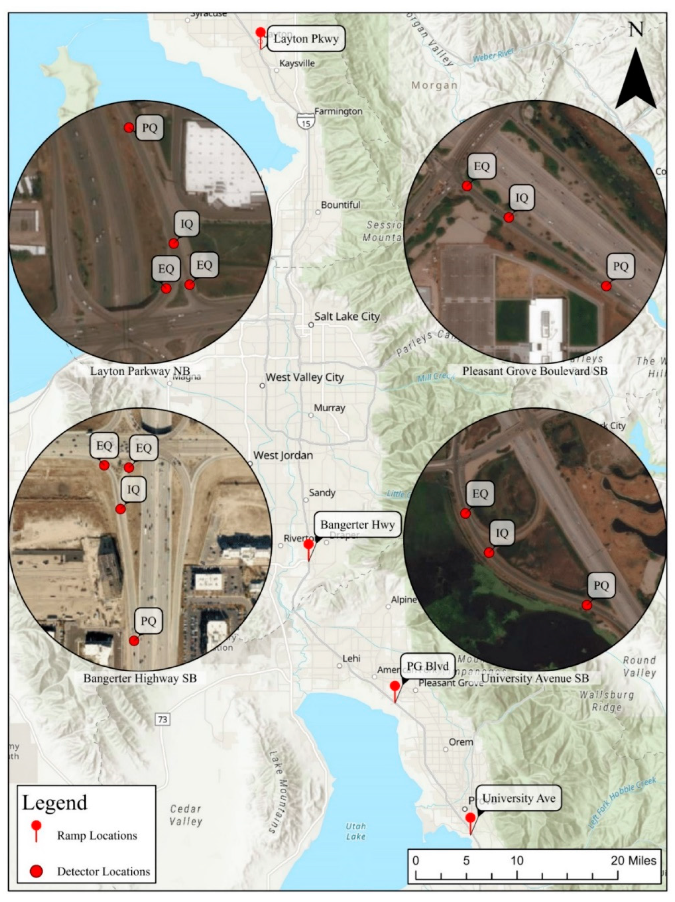
Four on-ramps to I-15 in Davis, Salt Lake, and Utah counties in Utah were chosen for data collection and analysis. These ramps include the northbound (NB) on-ramp at Layton Parkway in Davis County, the southbound (SB) on-ramp at Bangerter Highway in Salt Lake County, the SB on-ramp at Pleasant Grove Boulevard in Utah County, and the SB on-ramp at University Avenue in Utah County, as shown in
Figure 2. Data were collected during several periods in April and July 2021. Five weekdays of data (Monday through Friday) were collected at the four on-ramps during the PM metering period.
This section describes the data collection process at each of the four ramps studied in the research. A discussion will be presented on the time periods analyzed, the lane configuration and general characteristics of each ramp, the location of the loop detectors along the ramp, the data collected by the loop detectors, and the manually collected data.
4.1. Layton Parkway Northbound On-Ramp
The Layton Parkway NB on-ramp is located in the city of Layton in Davis County, Utah. At the entrance of the ramp, there are three receiving lanes, with two of these lanes used for the dual eastbound left turn lanes onto the ramp. The Layton Parkway and I-15 interchange is a single-point urban interchange and the eastbound left turn lanes operate with protected-only left turn phasing. The third entry lane on the on-ramp is used for the westbound right turn lane, which operates with free turning movement along Layton Parkway. However, approximately 150 feet upstream, westbound right turning vehicles must yield to the two lanes used for eastbound left turning vehicles as the ramp merges to two lanes approaching the ramp meter signal.
During the data collection periods, this ramp was metered during the PM peak period from 4:00 to 6:30 p.m. As shown in
Figure 2, there are EQ detectors in each of the three entry lanes located approximately 50 feet to the north of the ramp entrance. The IQ detectors are located in each lane shortly after the ramp merges from three to two lanes. Finally, PQ detectors are located immediately after the ramp meter signal, which is located approximately 540 feet to the north of the ramp entrance.
4.2. Bangerter Highway Southbound On-Ramp
The Bangerter Highway SB on-ramp is located in the city of Draper in Salt Lake County, Utah. At the entrance of the ramp, there are three receiving lanes, with two of these lanes used for the dual westbound left turn lanes onto the ramp. The Bangerter Highway and I-15 interchange is a single-point urban interchange and the westbound left turn lanes operate with protected-only left turn phasing. The third entry lane on the on-ramp is used for the eastbound right turn lane, which operates with free turning movement. These three entry lanes continue up through the ramp meter signal and then merge to two lanes shortly after the signal.
During the data collection periods, this ramp was metered during the PM peak period from 3:30 to 5:45 p.m. As shown in
Figure 2, there are EQ detectors in each of the three entry lanes located approximately 50 feet to the south of the ramp entrance. The IQ detectors are located in each lane approximately 250 feet to the south of the EQ detectors. Finally, PQ detectors are located immediately after the ramp meter signal, which is located approximately 1000 feet to the south of the ramp entrance.
4.3. Pleasant Grove Boulevard Southbound On-Ramp
The Pleasant Grove Boulevard SB on-ramp is located in the city of Pleasant Grove in Utah County, Utah. At the entrance of the ramp, there are two receiving lanes. At the intersection of Pleasant Grove Boulevard and the I-15 SB ramps, there are dual westbound left turn lanes onto the ramp and a shared eastbound through/right turn lane. The Pleasant Grove Boulevard and I-15 interchange is a diamond interchange and the westbound left turn lanes operate with protected-only left turn phasing. Eastbound right turning vehicles are controlled by the signalized intersection and are permitted to turn right on red after a stop, but they may be restricted at times as right turning vehicles may be blocked by vehicles traveling in the eastbound through direction in this shared through/right turn lane. These two entry lanes continue up through the ramp meter signal.
During the data collection periods, this ramp was metered during the PM peak period from 4:00 to 6:00 p.m. As shown in
Figure 2, there are EQ detectors in each of the entry lanes located approximately 50 feet to the south of the ramp entrance. The IQ detectors are located in each lane approximately 250 feet to the south of the EQ detectors. Finally, PQ detectors are located immediately after the ramp meter signal, which is located approximately 775 feet to the south of the ramp entrance.
4.4. University Avenue Southbound On-Ramp
The University Avenue SB on-ramp is located in the city of Provo in Utah County, Utah. The University Avenue and I-15 interchange is similar to what is typically known as a trumpet interchange. Of note, this interchange includes two different roadways, with University Avenue generally traveling in the north/south direction, and Lakeview Parkway/1860 South traveling in the east/west direction. The intersection prior to the ramp entrance includes a west leg known as Lakeview Parkway, the east leg known as 1860 South, the north leg stemming from University Avenue, and the south leg as the I-15 southbound on-ramp. As such, there are dual westbound left turn lanes on 1860 South, which operate with protected-only left turn phasing. There is an eastbound right turn lane on Lakeview Parkway from which vehicles may turn right on red after a stop. At the entrance of the ramp, there are three receiving lanes. These three entry lanes continue up through the ramp meter signal.
During the data collection periods, this ramp was metered during the PM peak period from 4:30 to 6:15 p.m. As shown in
Figure 2, there are EQ detectors in each of the entry lanes located approximately 325 feet to the south of the ramp entrance. The IQ detectors are located in each lane approximately 550 feet to the south of the EQ detectors. Finally, PQ detectors are located immediately after the ramp meter signal, which is located approximately 1875 feet to the south of the ramp entrance.
4.5. Loop Detector Data Collection
The EQ, IQ, and PQ detectors in each lane along the four studied ramps collect both volume and occupancy data and are automatically recorded in 60 s increments in the TransSuite system used by UDOT. As an example, the Layton Parkway NB Ramp has three EQ detectors, two IQ detectors, and two PQ detectors, one for each lane at their respective locations. These detectors provide volume estimates in each 60 s increment based on the detector of a vehicle crossing over the detector. In like manner, occupancy estimates are also provided in 60 s increments at each detector based on the percentage of time during that increment in which a vehicle was sensed above the detector (e.g., if vehicles were detected to be above the detector during 30 of 60 s, the occupancy at that detector in that time period would be 50 percent).
In addition, the variable ramp meter discharge rate (in units of veh/h) for each minute is included with the detector data. This discharge rate is for the overall ramp rather than a lane-by-lane discharge rate (e.g., if the ramp metering rate if 800 veh/h and there are two lanes at the ramp meter signal, the ramp meter discharge rate per lane is 400 veh/h/lane). The ramp meter discharge rate is determined by the ramp metering algorithm used by UDOT, which can automatically modify the ramp metering rate in each minute as needed based on perceived freeway and ramp conditions.
4.6. Field Collected Data
The manual data collection was performed by recording the on-ramps during the PM metering periods using UDOT cameras accessed in the Brigham Young University Transportation Lab. To align with the loop detector data, the manual data collection was also performed in 60 s increments. The field-collected data include the number of vehicles entering and exiting the ramp in each lane, the total number of vehicles on the ramp, the number of lanes on the ramp, and the vehicles queued at the ramp meter signal each minute.
5. Analysis Results
This section includes a discussion on the results of the optimized comparison, the linear regression models, and the cluster analysis based on their ability to estimate queue lengths as closely as the optimized values are able to achieve using observed data.
5.1. Optimized K Comparison
As discussed in the methodology section, the optimized
analysis was performed to provide a baseline for the other Kalman filter equation variations. The
produced for each 15 min period was not restricted to the range of 0 <
< 1, as was done in previous research [
8]. Rather,
was permitted to extend beyond this range of values based on the minimum RMSE found between the observed and modeled queue length estimates. The results of the optimized
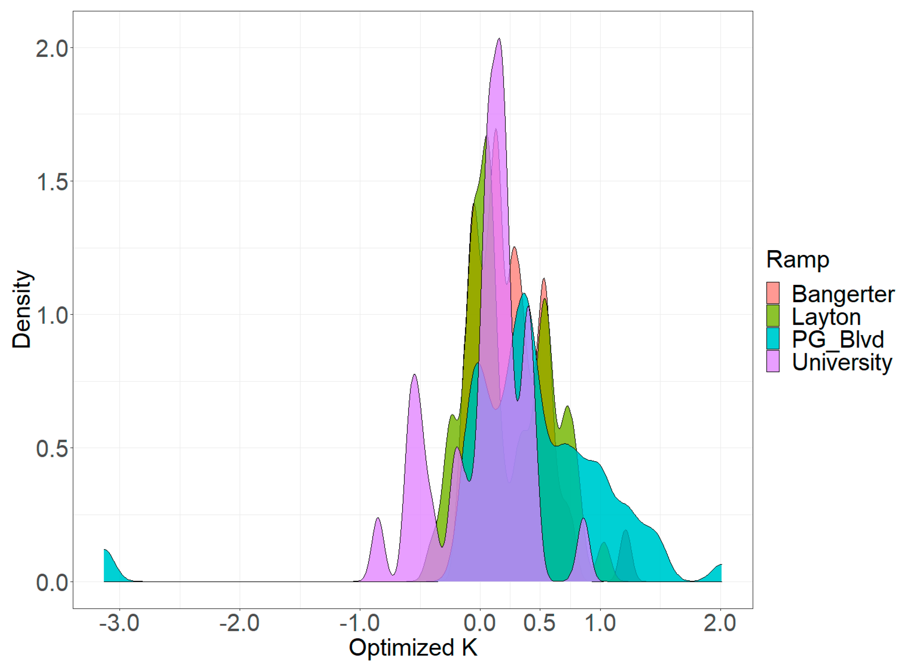
variation is illustrated in
Figure 3, which shows the frequency of different optimized
values for each 15 min period, organized by ramp. Although
does vary, the highest density of
values are between approximately 0 <
< 0.5.
5.2. Linear Regression Models
Linear regression models were used to develop an equation to predict
for any metering period. Many different linear regression models were tested, although just four primary models to predict
K are shown in
Table 1. In three of the four models, log transformations of the data were used to linearize the data. The variables that were log transformed included an additional factor of either 0.01 for the occupancy variables and 1 for the density variable to prevent these methods from producing errors if the occupancy or density were 0 at any point within the dataset, as log(0) is undefined.
The four linear regression models to predict K included in this analysis are as follows:
Ramp Control [Density]: the inputs of this model include the IQ occupancy, a log transformation of the density, and a variable for ramp control.
Ramp Control [Occ.]: the inputs of this model focus primarily on the three detector locations and include the IQ, EQ, and PQ occupancy, in addition to a variable for ramp control.
Ramp Control [Log Occ.]: this model used the same inputs as “Ramp Control [Occ.]” but used a log transformation of each occupancy value.
Log Occ. [No Ramp]: this model used only a log transformation of each occupancy value, with no variable for ramp control, in other words, the output equation would result in the same value for each ramp.
The Ramp Control [Density] model was selected for use in comparison against the optimized
model, as this model yielded the best results with respect to the R
2 value (closer to 1) and the log likelihood (closer to 0) versus the different linear regression models shown in
Table 1. The equation for
K that would be produced by the Ramp Control [Density] model is shown in Equations (11)–(14), which has a unique final term in each equation dependent on which ramp is being used. Equation (11) is for Bangerter Highway, Equation (12) for Layton Parkway, Equation (13) for Pleasant Grove Boulevard, and Equation (14) for University Avenue.
where:
5.3. Cluster Analysis and Heuristic Models
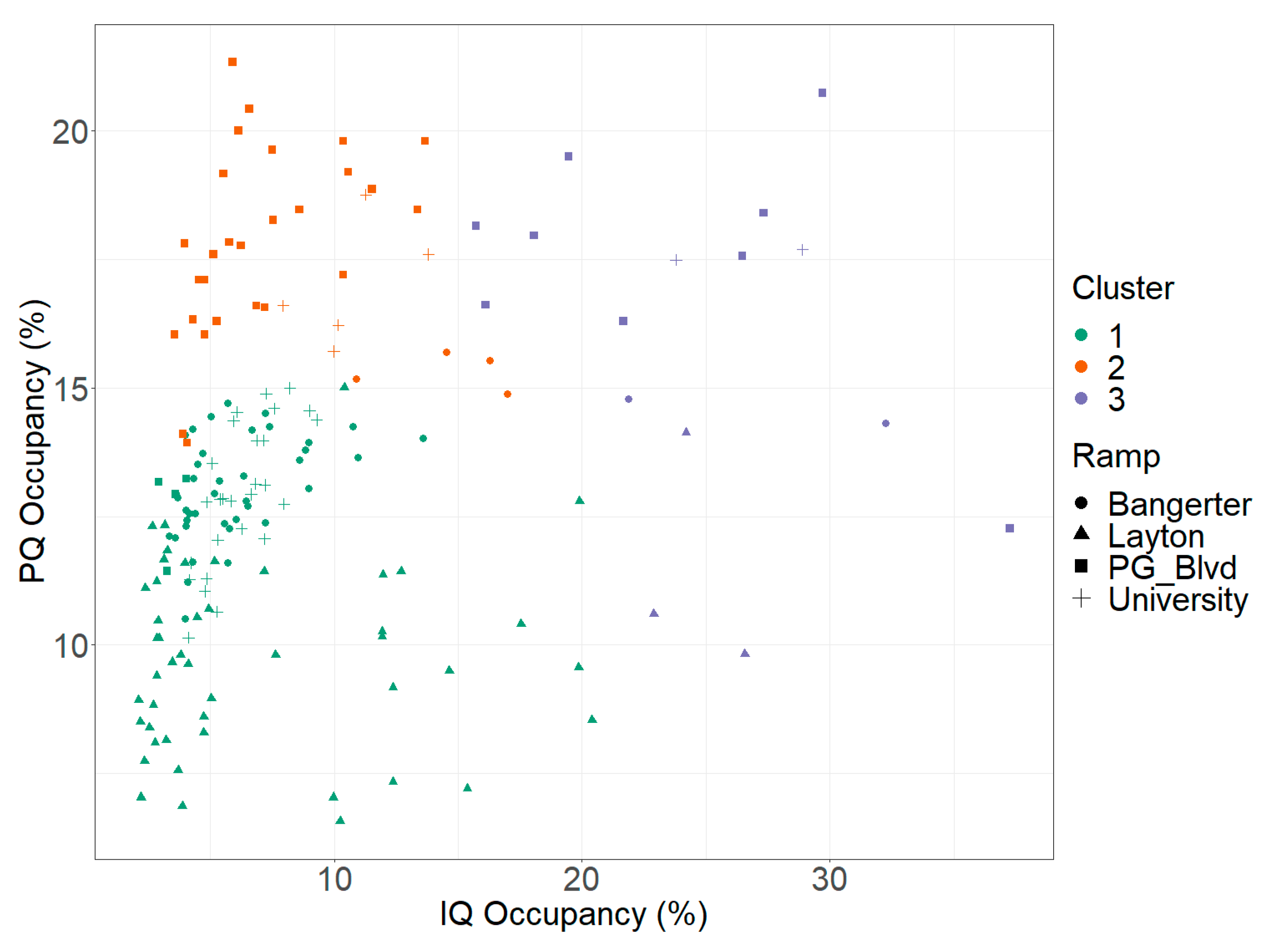
For the cluster analysis performed in this research, the PQ occupancy was compared to the IQ occupancy for each 15 min period. Each 15 min period represented one data point and had its own value. Three clusters were used in the analysis, as the use of fewer or more clusters reduced its usefulness either in variability or prevented each cluster from having an adequate sample size to be reliable. From the cluster analysis, the average of all data points within each cluster was calculated and then that was applied across all data points for each respective cluster.
The average
, the number of observations (n), and the standard deviation (SD) of the data points were calculated for each cluster. Cluster 1, as it is designated in
Figure 4, pertains to those time periods where there were both a low PQ and a low IQ occupancy. Cluster 2 represents data points with a high PQ occupancy and low IQ occupancy, while Cluster 3 captures data points that had a high IQ occupancy and either a high or low PQ occupancy.
From
Figure 4, cutoff ranges were developed based on the cluster analysis that most approximately captured the data points within each of the three clusters, with the cutoff between Cluster 1 and Cluster 2 occurring at 13.5 percent PQ occupancy, while the cutoff between Clusters 1 and 2 versus Cluster 3 was set at 16.0 percent IQ occupancy. Therefore, any data point that fell within Cluster 1 would be given a uniform
of 0.189 (
n = 93, SD = 0.400), while Cluster 2 would be assigned a
of 0.337 (
n = 56, SD = 0.439), and Cluster 3 would have a
of 0.170 (
n = 20, SD = 0.833).
Figure 4 shows a plot of the cluster analysis with each of the clusters shown by color, while also having unique shapes to designate the ramp to which each data point belongs. With this information, a heuristic model was developed to predict the queue length of vehicles at the metered on-ramp based on the detector occupancy.
5.4. Queue Length Analysis
The queue length estimates were generated using several variations of the Kalman filter algorithm presented in the Analysis Methodology section, including an optimized comparison, a conservation model, the Vigos model, a heuristic model, and a linear regression model. The optimized comparison method was used as a baseline for the other models because it is the closest any Kalman filter model comes to the actual queue length.
The value was calibrated for each 15 min period on each ramp and for each day by minimizing the RMSE between the field recorded queue length and the estimated queue length from the Kalman filter algorithm. Each of these models was then compared with the field recorded queue length to determine which model most closely resembled the actual queue length.
Each model was assigned a value based on the criteria set for each model. The optimized would have varied values per ramp every 15 min, dependent on which value produced the minimum RMSE between the observed and modeled queue length. The conservation model used a constant value of 0 for for all time periods on all ramps. The Vigos model used a constant value of 0.22 for for all time periods on all ramps. The heuristic model used a cluster analysis that produced three possible values that could be selected per ramp for each 15 min period depending on where that period fit in the cluster analysis. Finally, the linear regression model produced an equation that calculated for each 15 min period.
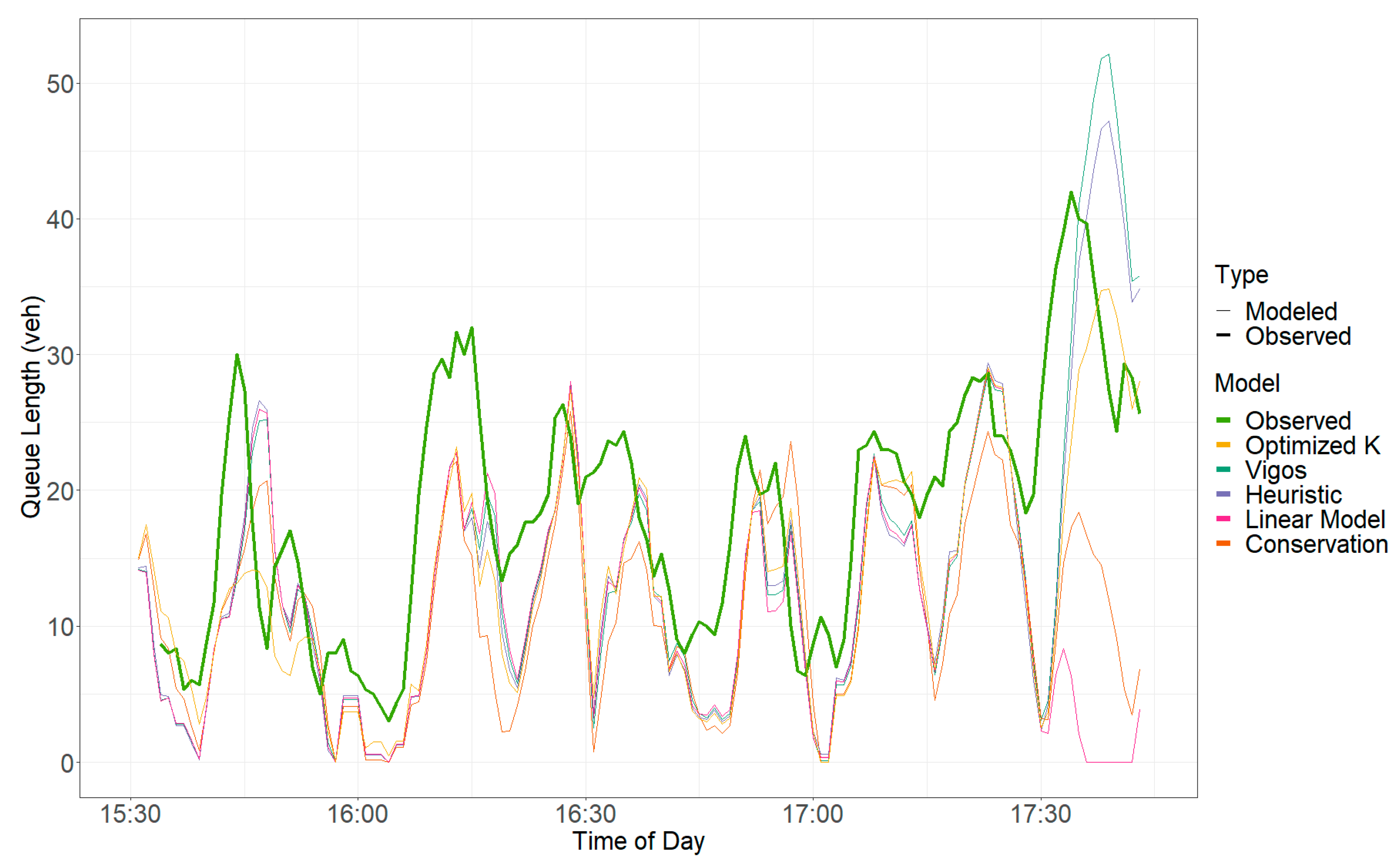
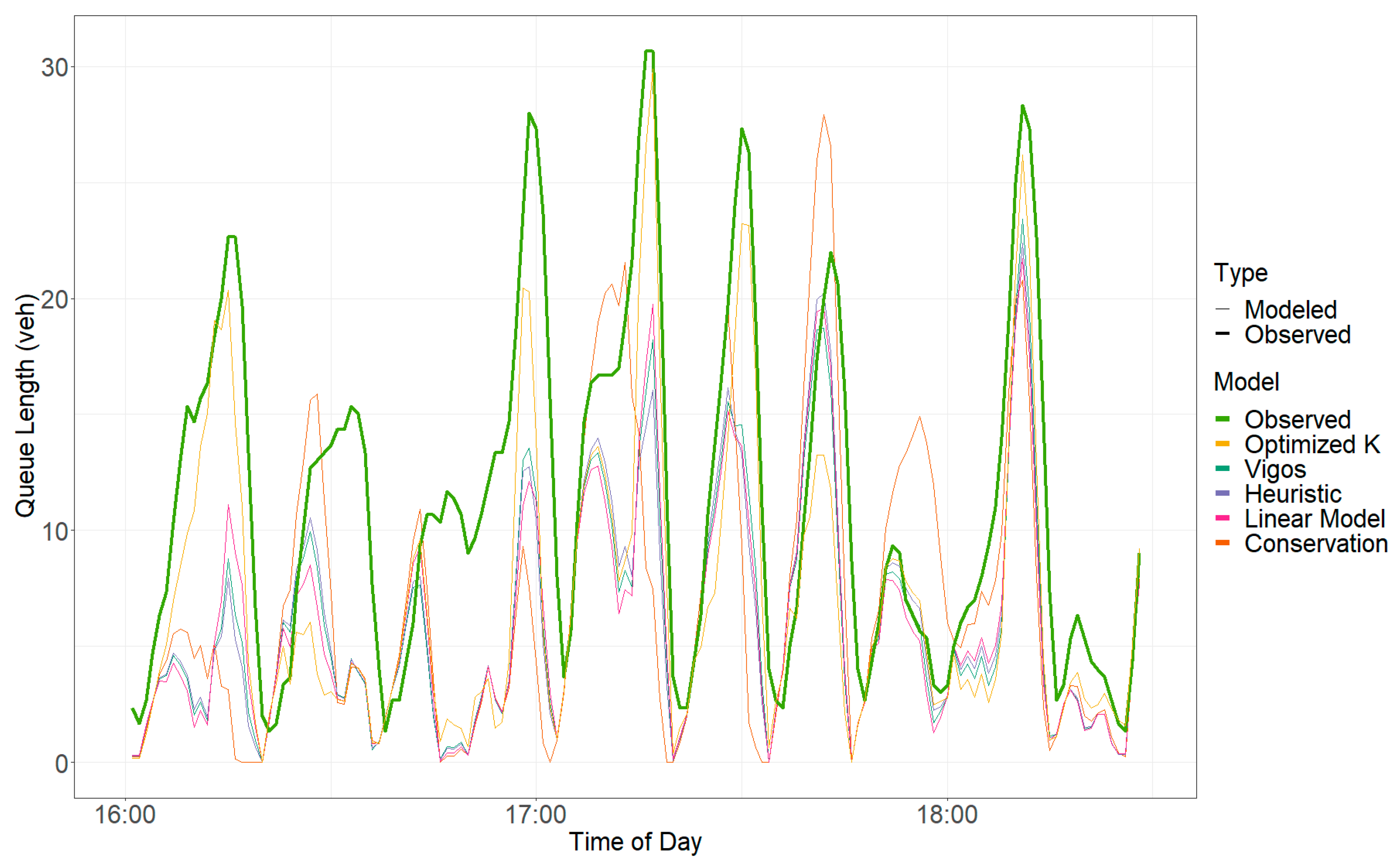
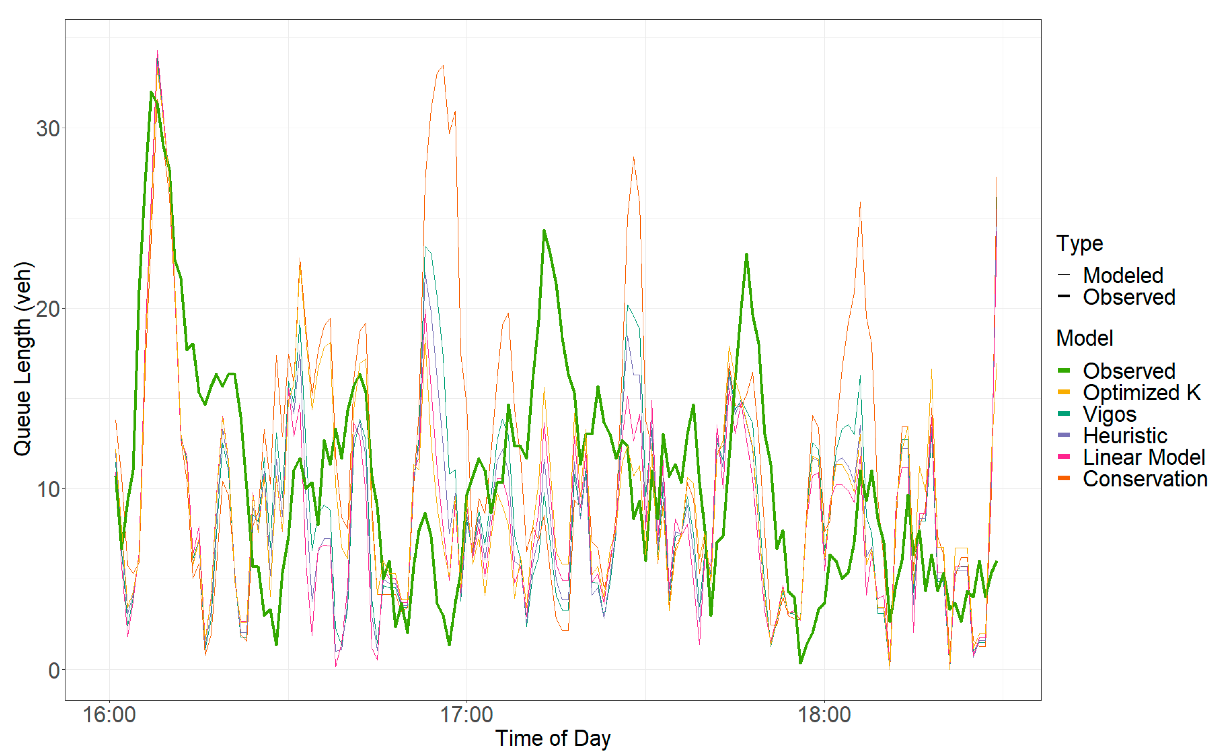
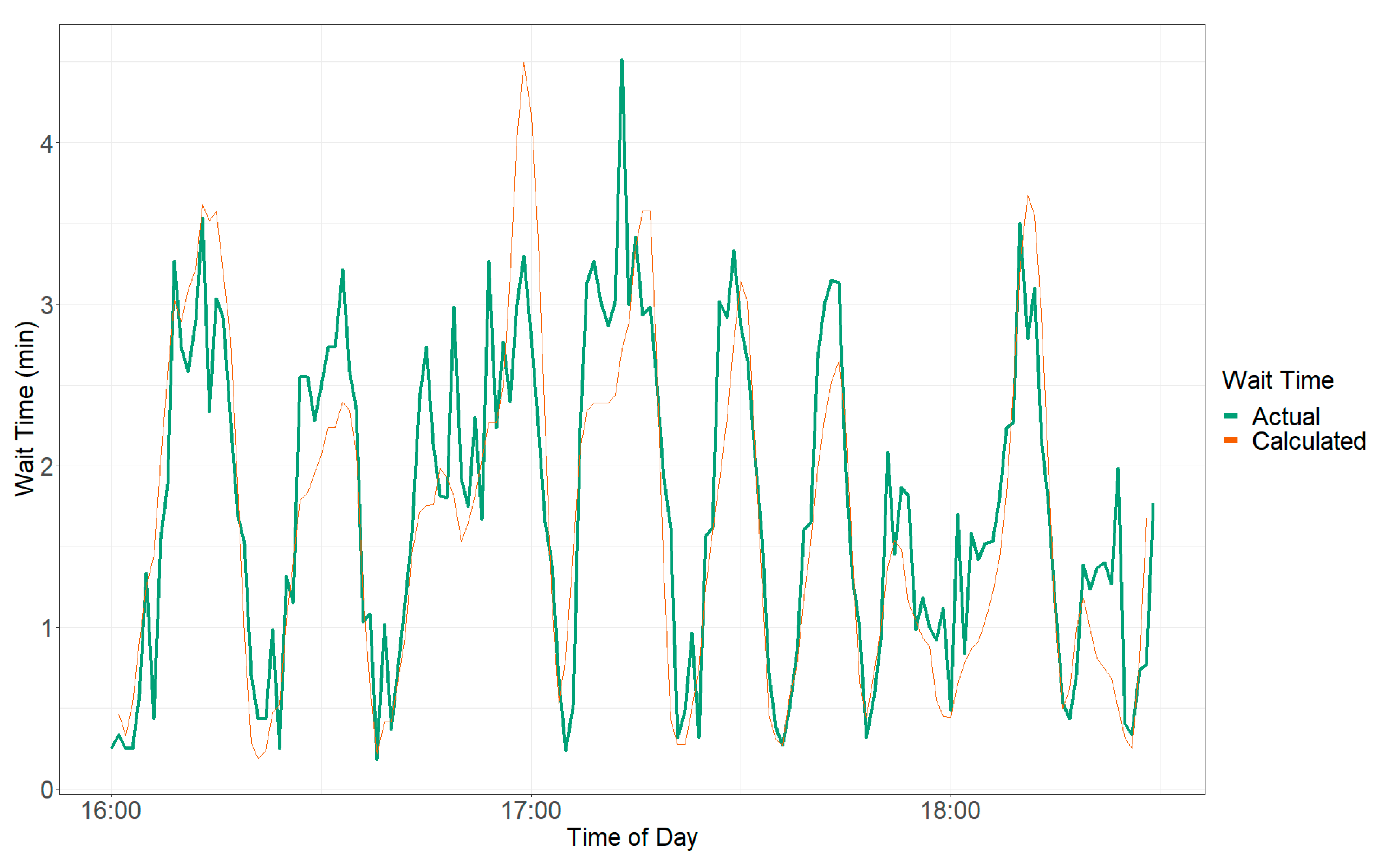
The queue length estimates compared against each other during the PM metering period are shown in
Figure 5,
Figure 6,
Figure 7 and
Figure 8 for Bangerter Highway SB, Layton Parkway NB, Pleasant Grove Boulevard SB, and University Avenue SB, respectively. The thicker line, called “Observed,” represents the field-recorded queue length, which is the target line that the modeled queue lengths seek to represent. Only one day of the five days that were collected for each ramp is shown for conciseness, but each ramp experienced similar patterns with respect to the accuracy of the models against the field recorded queue length throughout each day. Full model results can be found in the literature [
32].
Because each of the models analyzed are variations of the same Kalman filter equation, the models generally follow each other along a similar path, with some variation occurring in the queue length estimates attributed to the variation in
. There is some variation in the quality of each model in reflecting the observed queue length. This is particularly evident in the linear regression and conservation models shown in
Figure 5,
Figure 6,
Figure 7 and
Figure 8, while the Vigos and heuristic models generally follow the observed queue length more closely.
Although not all ramps perform equally, the heuristic and Vigos models more closely follow the observed queue length and are within approximately 10 vehicles throughout each day.
Table 2 shows the reported RMSE for each of the models that were analyzed for the entire dataset as well as the RMSE calculated for each ramp. The RMSE was calculated by comparing the modeled queue length against the observed queue length for each period. The optimized
method minimizes the RMSE between the field-recorded and the modeled queue lengths and is thus used as a baseline for comparison. Although recognizably the most accurate model at predicting the actual queue length at each ramp, the optimized
baseline cannot be used in practice without calibration through field data collection. As such, this method—the generally analyzed method used in previous research—does not provide usable results for continual use and application [
3,
7,
8,
9].
While the order of RMSE varies slightly by ramp, the heuristic model generally performs best when using the RMSE as the comparison mechanism. The heuristic model is based on a cluster analysis that yielded three possible values for . However, the Vigos model, which uses a constant value of 0.22, performs nearly as well—if not sometimes better than—the heuristic model. The Vigos model was most closely aligned with the average that was calculated for the four ramps used in this research, which was computed to be 0.22, matching the value found in the Vigos model.
The heuristic model and Vigos model have both proven to come close to the observed queue length at each ramp. These models are also able to capture the peaks and valleys of the queue that occur throughout the metering period by using the Kalman filter equation at each of the four ramps and from queue lengths ranging from as little as no queue to as many as approximately 70 vehicles.
5.5. Wait Time Analysis
To perform the wait time analysis at each ramp, the modeled and observed queue lengths (veh) were divided by the metering rate (veh/min) to generate the wait time in minutes as shown in Equation (15). This method was used because of its simplicity in using existing data that is provided by the detectors on each ramp.
where:
A field verification was completed at Layton Parkway to ensure that this method was reliable by manually measuring the wait time in 60 s increments—measuring the time elapsed from when a vehicle entered the ramp until it passed the ramp meter signal. The field recorded queue length was divided by the metering rate to compute the calculated wait time. The field recorded wait times were then compared to the wait time estimates calculated from Equation (15), as shown in
Figure 9.
Figure 9 shows that the calculated wait times follow the actual wait times quite well, as nearly every peak and valley throughout the day is captured, and the calculated wait times are generally never more than 30 s above or below the actual wait times during any given minute for this specific application. Therefore, it appears that using the metering rate to convert from queue length into wait time is a reasonable application. In estimating the wait times more broadly, most models used in this research across all ramps and periods throughout each day do tend to slightly underestimate the wait times produced by the conversion used in Equation (15).
