
State-of-the-Art Explainability Methods with Focus on Visual Analytics Showcased by Glioma Classification

 , , , ,
  , and
, and
Abstract
:1. Introduction
1.1. Classification of Diffuse Glioma
1.2. Theoretical Background on xAI
2. Materials and Methods
2.1. Dataset
2.2. Implementation
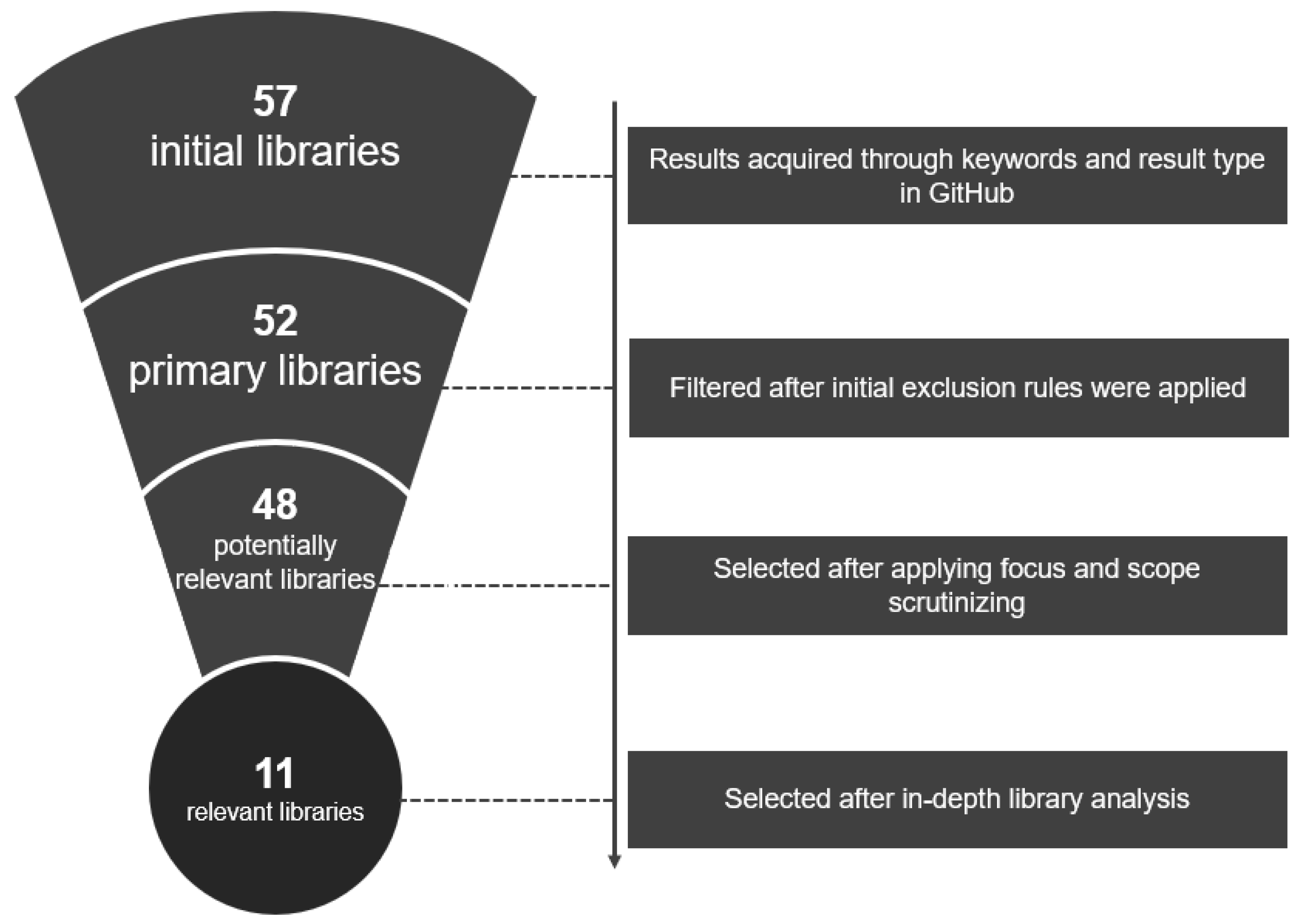
- 1.
- Result has to be a repository of a Python library or a software package;
- 2.
- Result has to implement at least one xAI method;
- 3.
- Result has to be an overview repository (repository that provides an overview of xAI libaries).
3. Results
3.1. Library Comparison on Glioma Subtype Classification
3.2. Python Libraries for Explainability
3.3. Global Explainability
3.4. Local Explainability
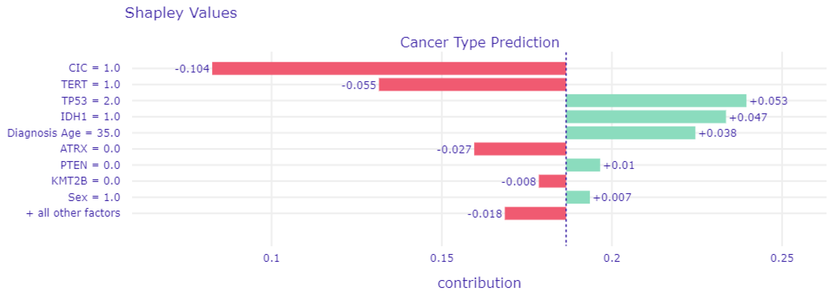
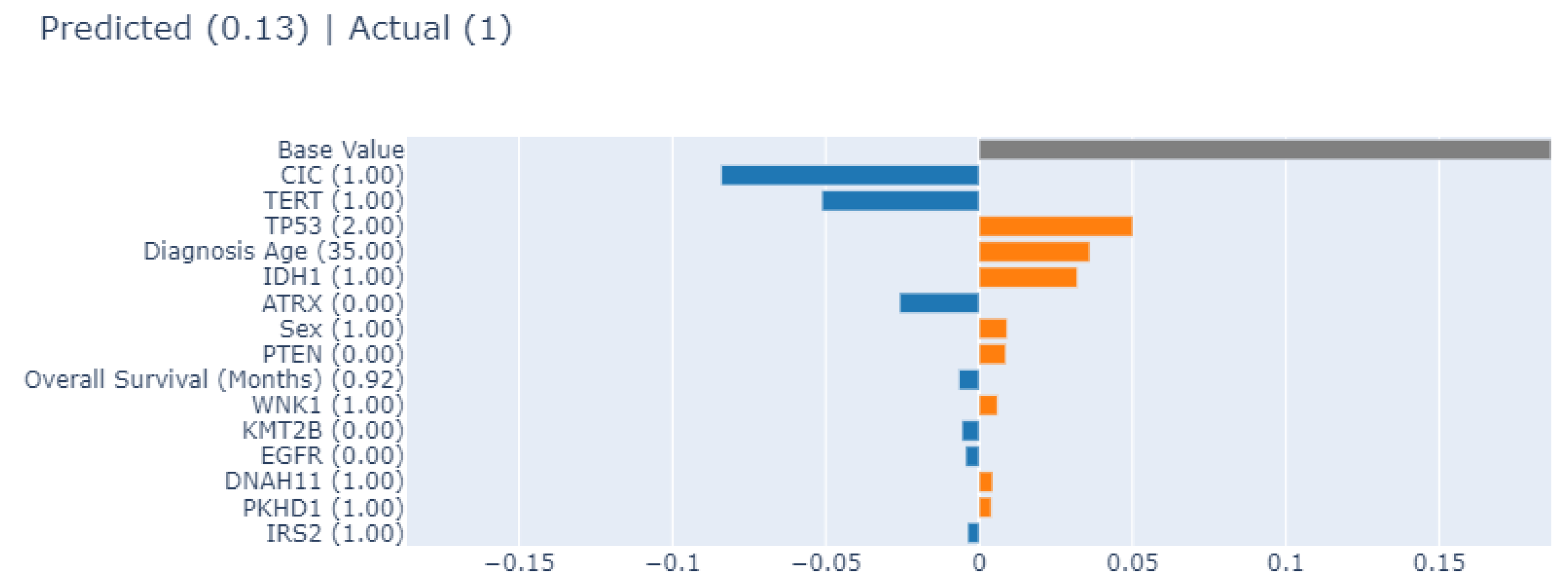
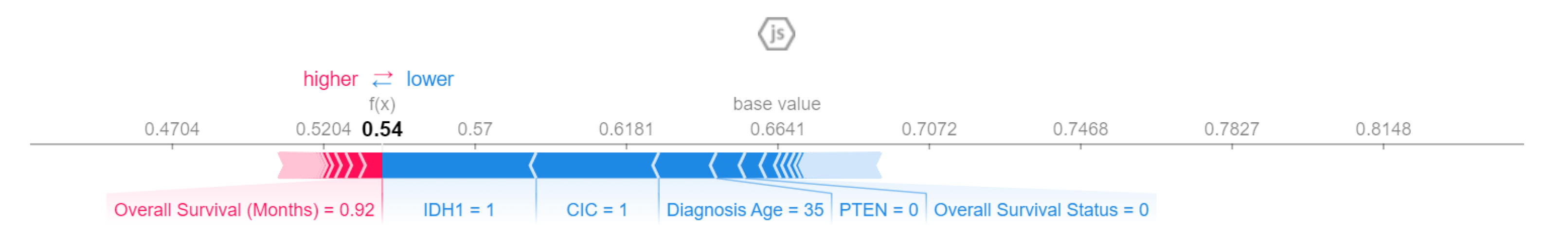
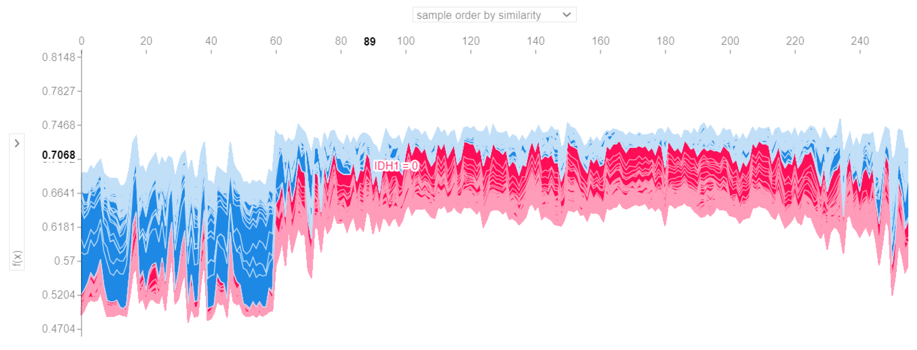
3.4.1. Local Explainability with SHAP
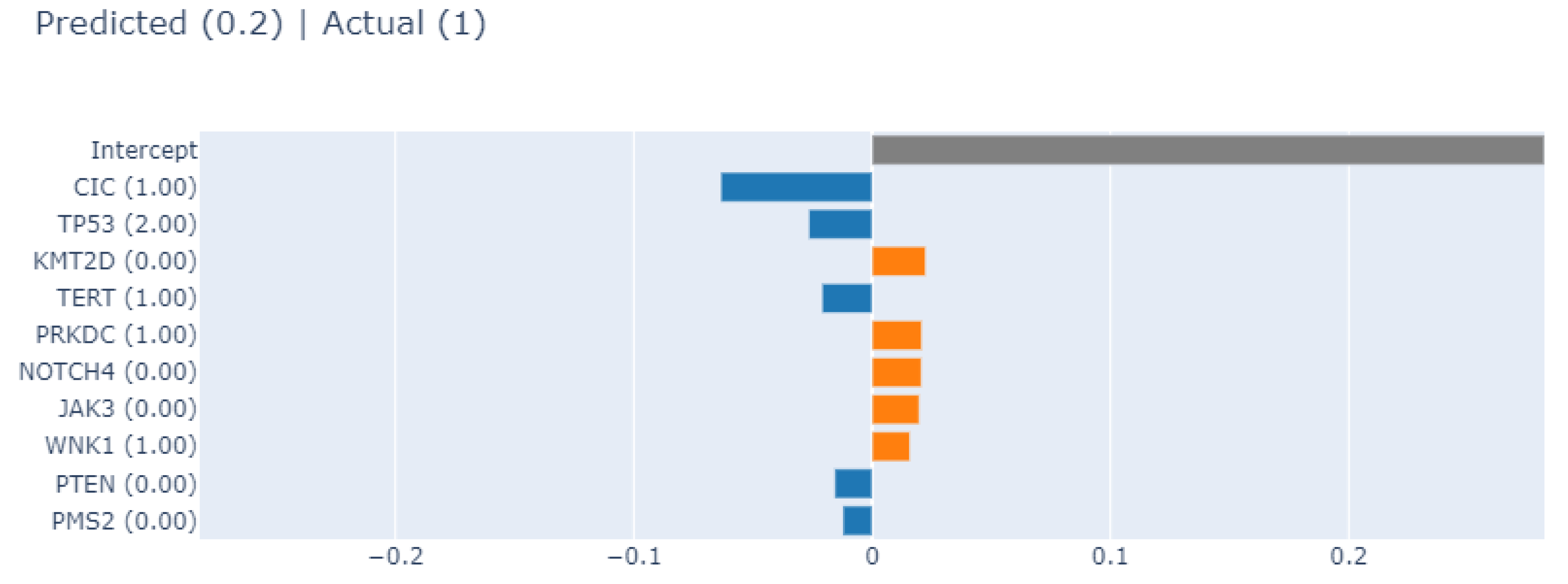
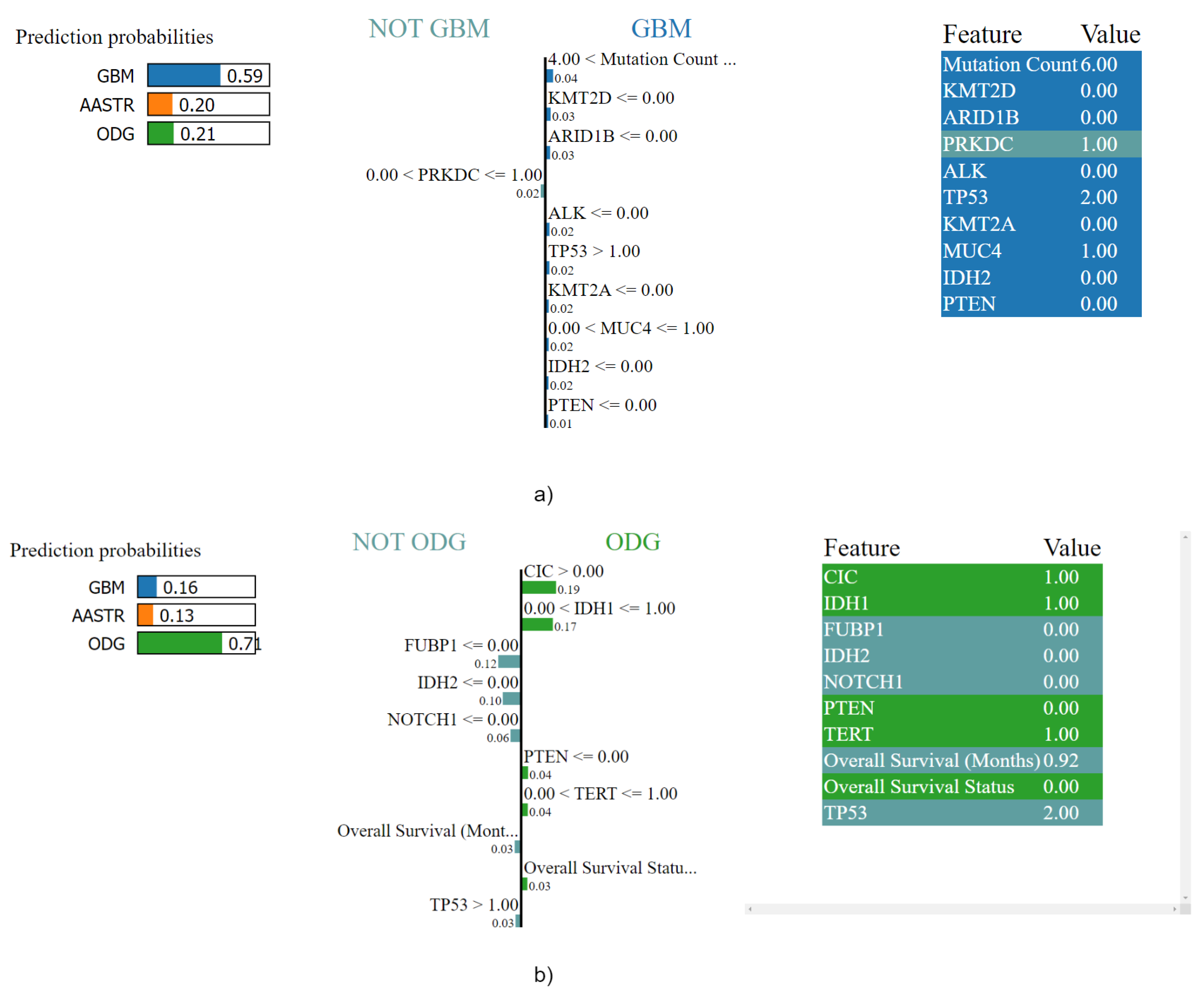
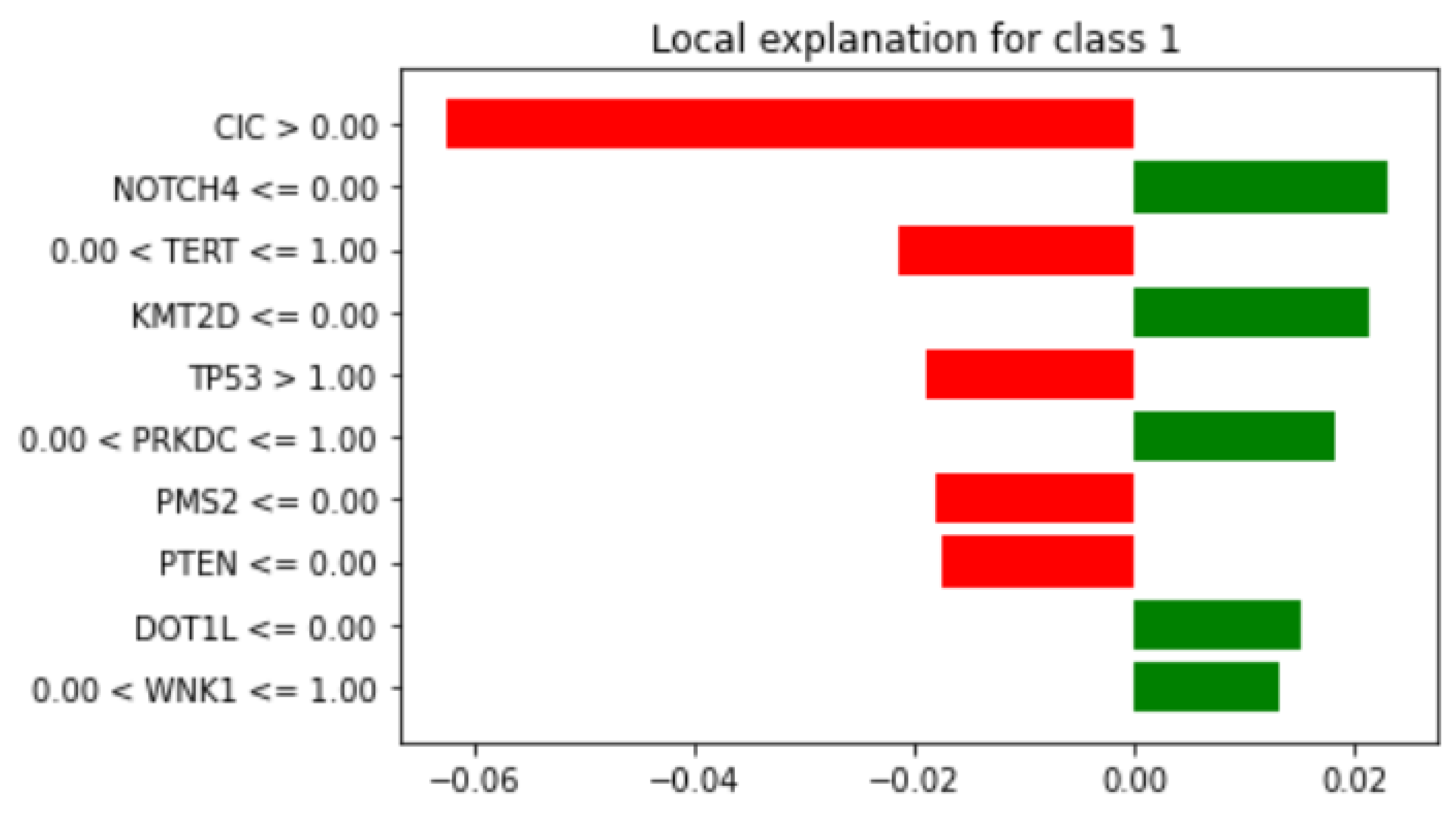
3.4.2. Local Explainability with LIME
3.5. Biomedical Implication of Features
3.6. Overview of xAI Approaches
4. Discussion
5. Conclusions
Author Contributions
Funding
Institutional Review Board Statement
Informed Consent Statement
Data Availability Statement
Acknowledgments
Conflicts of Interest
Abbreviations
| AASTR | Anaplastic Astrocytoma |
| DIFG | Diffuse Glioma |
| CIC | Capicua gene |
| GBM | Glioblastoma multiforme |
| LIME | Local Interpretable Model-Agnostic Explanations |
| ODG | Oligodendroglioma |
| SHAP | SHapley Additive exPlanations |
| VA | Visual Analytics |
| xAI | explainable Artificial Intelligence |
Appendix A
Appendix A.1. Complete Table of All Identified xAI Libraries
Appendix A.2. Implementation Details
References
- Bhardwaj, R.; Nambiar, A.R.; Dutta, D. A study of machine learning in healthcare. In Proceedings of the 2017 IEEE 41st Annual Computer Software and Applications Conference (COMPSAC), Turin, Italy, 4–8 July 2017; Volume 2, pp. 236–241. [Google Scholar]
- Guyon, I.; Weston, J.; Barnhill, S.; Vapnik, V. Gene selection for cancer classification using support vector machines. Mach. Learn. 2002, 46, 389–422. [Google Scholar] [CrossRef]
- Galon, J.; Pagès, F.; Marincola, F.M.; Angell, H.K.; Thurin, M.; Lugli, A.; Zlobec, I.; Berger, A.; Bifulco, C.; Botti, G.; et al. Cancer classification using the Immunoscore: A worldwide task force. J. Transl. Med. 2012, 10, 1–10. [Google Scholar] [CrossRef] [PubMed]
- Murtaza, G.; Shuib, L.; Abdul Wahab, A.W.; Mujtaba, G.; Nweke, H.F.; Al-garadi, M.A.; Zulfiqar, F.; Raza, G.; Azmi, N.A. Deep learning-based breast cancer classification through medical imaging modalities: State of the art and research challenges. Artif. Intell. Rev. 2020, 53, 1655–1720. [Google Scholar] [CrossRef]
- Carrio, A.; Sampedro, C.; Rodriguez-Ramos, A.; Campoy, P. A review of deep learning methods and applications for unmanned aerial vehicles. J. Sens. 2017, 2017, 3296874. [Google Scholar] [CrossRef]
- Razzak, M.I.; Naz, S.; Zaib, A. Deep learning for medical image processing: Overview, challenges and the future. In Classification in BioApps; Springer: Cham, Switzerland, 2018; pp. 323–350. [Google Scholar]
- Vukovi´c, M.; Thalmann, S. Causal Discovery in Manufacturing: A Structured Literature Review. J. Manuf. Mater. Process 2022, 6, 10. [Google Scholar] [CrossRef]
- Gashi, M.; Ofner, P.; Ennsbrunner, H.; Thalmann, S. Dealing with missing usage data in defect prediction: A case study of a welding supplier. Comput. Ind. 2021, 132, 103505. [Google Scholar] [CrossRef]
- Holzinger, A.; Kieseberg, P.; Weippl, E.; Tjoa, A.M. Current Advances, Trends and Challenges of Machine Learning and Knowledge Extraction: From Machine Learning to Explainable AI. In Machine Learning and Knowledge Extraction; Holzinger, A., Kieseberg, P., Tjoa, A.M., Weippl, E., Eds.; Springer International Publishing: Cham, Siwitzerland, 2018; pp. 1–8. [Google Scholar]
- Holzinger, A.; Goebel, R.; Mengel, M.; Müller, H. Artificial Intelligence and Machine Learning for Digital Pathology: State-of-the-Art and Future Challenges; Springer Nature: Cham, Switzerland, 2020; Volume 12090. [Google Scholar]
- Adadi, A.; Berrada, M. Peeking inside the black-box: A survey on explainable artificial intelligence (XAI). IEEE Access 2018, 6, 52138–52160. [Google Scholar] [CrossRef]
- Castelvecchi, D. Can we open the black box of AI? Nat. News 2016, 538, 20. [Google Scholar] [CrossRef] [Green Version]
- Samek, W.; Montavon, G.; Vedaldi, A.; Hansen, L.K.; Müller, K.R. Explainable AI: Interpreting, Explaining and Visualizing Deep Learning; Springer Nature: Cham, Switzerland, 2019; Volume 11700. [Google Scholar]
- Königstorfer, F.; Thalmann, S. Software documentation is not enough! Requirements for the documentation of AI. Digit. Policy Regul. Gov. 2021, 23, 475–488. [Google Scholar] [CrossRef]
- Polzer, A.; Fleiß, J.; Ebner, T.; Kainz, P.; Koeth, C.; Thalmann, S. Validation of AI-based Information Systems for Sensitive Use Cases: Using an XAI Approach in Pharmaceutical Engineering. In Proceedings of the 55th Hawaii International Conference on System Sciences, Maui, HI, USA, 4–7 January 2022. [Google Scholar]
- Ribeiro, M.T.; Singh, S.; Guestrin, C. “Why should i trust you?” Explaining the predictions of any classifier. In Proceedings of the 22nd ACM SIGKDD International Conference on Knowledge Discovery and Data Mining, San Francisco, CA, USA, 13–17 August 2016; pp. 1135–1144. [Google Scholar]
- Lundberg, S.M.; Lee, S.I. A Unified Approach to Interpreting Model Predictions. In Advances in Neural Information Processing Systems 30; Guyon, I., Luxburg, U.V., Bengio, S., Wallach, H., Fergus, R., Vishwanathan, S., Garnett, R., Eds.; Curran Associates, Inc.: Red Hook, NY, USA, 2017; pp. 4765–4774. [Google Scholar]
- Holzinger, A.; Biemann, C.; Pattichis, C.S.; Kell, D.B. What do we need to build explainable AI systems for the medical domain? arXiv 2017, arXiv:1712.09923. [Google Scholar]
- Katuwal, G.J.; Chen, R. Machine learning model interpretability for precision medicine. arXiv 2016, arXiv:1610.09045. [Google Scholar]
- Jiarpakdee, J.; Tantithamthavorn, C.; Dam, H.K.; Grundy, J. An empirical study of model-agnostic techniques for defect prediction models. IEEE Trans. Softw. Eng. 2020, 48, 166–185. [Google Scholar] [CrossRef]
- Tan, S.; Caruana, R.; Hooker, G.; Lou, Y. Detecting bias in black-box models using transparent model distillation. arXiv 2017, arXiv:1710.06169. [Google Scholar]
- Jean-Quartier, C.; Jeanquartier, F.; Ridvan, A.; Kargl, M.; Mirza, T.; Stangl, T.; Markaĉ, R.; Jurada, M.; Holzinger, A. Mutation-based clustering and classification analysis reveals distinctive age groups and age-related biomarkers for glioma. BMC Med. Inform. Decis. Mak. 2021, 21, 1–14. [Google Scholar] [CrossRef] [PubMed]
- Xu, K.; Ba, J.; Kiros, R.; Cho, K.; Courville, A.; Salakhudinov, R.; Zemel, R.; Bengio, Y. Show, attend and tell: Neural image caption generation with visual attention. In Proceedings of the International Conference on Machine Learning, Lille, France, 6–11 July 2015; pp. 2048–2057. [Google Scholar]
- Keim, D.A.; Mansmann, F.; Stoffel, A.; Ziegler, H. Visual analytics. In Encyclopedia of Database Systems; Springer: Berlin/Heidelberg, Germany, 2009. [Google Scholar]
- Samek, W.; Wiegand, T.; Müller, K.R. Explainable artificial intelligence: Understanding, visualizing and interpreting deep learning models. arXiv 2017, arXiv:1708.08296. [Google Scholar]
- Gashi, M.; Mutlu, B.; Suschnigg, J.; Ofner, P.; Pichler, S.; Schreck, T. Interactive Visual Exploration of defect prediction in industrial setting through explainable models based on SHAP values. In Proceedings of the IEEE InfoVIS 2020, Virtuell, MZ, USA, 25–30 October 2020. [Google Scholar]
- Spinner, T.; Schlegel, U.; Schäfer, H.; El-Assady, M. explAIner: A visual analytics framework for interactive and explainable machine learning. IEEE Trans. Vis. Comput. Graph. 2019, 26, 1064–1074. [Google Scholar] [CrossRef] [PubMed] [Green Version]
- Nori, H.; Jenkins, S.; Koch, P.; Caruana, R. InterpretML: A Unified Framework for Machine Learning Interpretability. arXiv 2019, arXiv:1909.09223. [Google Scholar]
- Baniecki, H.; Kretowicz, W.; Piatyszek, P.; Wisniewski, J.; Biecek, P. Dalex: Responsible Machine Learning with Interactive Explainability and Fairness in Python. arXiv 2020, arXiv:2012.14406. [Google Scholar]
- Li, X.H.; Cao, C.C.; Shi, Y.; Bai, W.; Gao, H.; Qiu, L.; Wang, C.; Gao, Y.; Zhang, S.; Xue, X.; et al. A survey of data-driven and knowledge-aware explainable AI. IEEE Trans. Knowl. Data Eng. 2020, 34, 29–49. [Google Scholar] [CrossRef]
- Linardatos, P.; Papastefanopoulos, V.; Kotsiantis, S. Explainable AI: A review of machine learning interpretability methods. Entropy 2021, 23, 18. [Google Scholar] [CrossRef] [PubMed]
- Vilone, G.; Longo, L. Explainable Artificial Intelligence: A Systematic Review. arXiv 2020, arXiv:2006.00093. [Google Scholar]
- Masui, K.; Mischel, P.S.; Reifenberger, G. Molecular classification of gliomas. Handb. Clin. Neurol. 2016, 134, 97–120. [Google Scholar] [PubMed]
- Louis, D.N.; Perry, A.; Wesseling, P.; Brat, D.J.; Cree, I.A.; Figarella-Branger, D.; Hawkins, C.; Ng, H.; Pfister, S.M.; Reifenberger, G.; et al. The 2021 WHO classification of tumors of the central nervous system: A summary. Neuro-Oncology 2021, 23, 1231–1251. [Google Scholar] [CrossRef] [PubMed]
- Kundra, R.; Zhang, H.; Sheridan, R.; Sirintrapun, S.J.; Wang, A.; Ochoa, A.; Wilson, M.; Gross, B.; Sun, Y.; Madupuri, R.; et al. OncoTree: A cancer classification system for precision oncology. JCO Clin. Cancer Inform. 2021, 5, 221–230. [Google Scholar] [CrossRef]
- Komori, T. Grading of adult diffuse gliomas according to the 2021 WHO Classification of Tumors of the Central Nervous System. Lab. Investig. 2021, 67, 1–8. [Google Scholar] [CrossRef]
- Zacher, A.; Kaulich, K.; Stepanow, S.; Wolter, M.; Köhrer, K.; Felsberg, J.; Malzkorn, B.; Reifenberger, G. Molecular diagnostics of gliomas using next generation sequencing of a glioma-tailored gene panel. Brain Pathol. 2017, 27, 146–159. [Google Scholar] [CrossRef]
- Van Lent, M.; Fisher, W.; Mancuso, M. An Explainable Artificial Intelligence System for Small-Unit Tactical Behavior; AAAI Press: Palo Alto, CA, USA, 1994; pp. 900–907. [Google Scholar]
- Shin, D.; Park, Y.J. Role of fairness, accountability, and transparency in algorithmic affordance. Comput. Hum. Behav. 2019, 98, 277–284. [Google Scholar] [CrossRef]
- Cerami, E.; Gao, J.; Dogrusoz, U.; Gross, B.E.; Sumer, S.O.; Aksoy, B.A.; Jacobsen, A.; Byrne, C.J.; Heuer, M.L.; Larsson, E.; et al. The cBio cancer genomics portal: An open platform for exploring multidimensional cancer genomics data. Cancer Discov. 2012, 2, 401–404. [Google Scholar] [CrossRef] [Green Version]
- Gao, J.; Aksoy, B.A.; Dogrusoz, U.; Dresdner, G.; Gross, B.; Sumer, S.O.; Sun, Y.; Jacobsen, A.; Sinha, R.; Larsson, E.; et al. Integrative analysis of complex cancer genomics and clinical profiles using the cBioPortal. Sci. Signal. 2013, 6, pl1. [Google Scholar] [CrossRef] [Green Version]
- Webster, J.; Watson, R.T. Analyzing the past to prepare for the future: Writing a literature review. MIS Q. 2002, 26, xiii–xxiii. [Google Scholar]
- ELI5’s Documentation. Available online: https://eli5.readthedocs.io/en/latest/overview.html (accessed on 12 January 2022).
- Fisher, A.; Rudin, C.; Dominici, F. All Models are Wrong, but Many are Useful: Learning a Variable’s Importance by Studying an Entire Class of Prediction Models Simultaneously. J. Mach. Learn. Res. 2019, 20, 1–81. [Google Scholar]
- Databricks. Collaborative Data Science; Databricks: San Francisco, CA, USA, 2015. [Google Scholar]
- Shapley, L.S.; Kuhn, H.; Tucker, A. Contributions to the Theory of Games. Ann. Math. Stud. 1953, 28, 307–317. [Google Scholar]
- Kleppe, A.; Skrede, O.J.; De Raedt, S.; Liestøl, K.; Kerr, D.J.; Danielsen, H.E. Designing deep learning studies in cancer diagnostics. Nat. Rev. Cancer 2021, 21, 199–211. [Google Scholar] [CrossRef]
- McCoy, L.G.; Brenna, C.T.; Chen, S.S.; Vold, K.; Das, S. Believing in black boxes: Machine learning for healthcare does not need explainability to be evidence-based. J. Clin. Epidemiol. 2021. [CrossRef]
- Wang, F.; Kaushal, R.; Khullar, D. Should health care demand interpretable artificial intelligence or accept “black box” medicine? Lab Investig. 2020. [CrossRef]
- Jeanquartier, F.; Jean-Quartier, C.; Stryeck, S.; Holzinger, A. Open Data to Support CANCER Science—A Bioinformatics Perspective on Glioma Research. Onco 2021, 1, 219–229. [Google Scholar] [CrossRef]
- Bunda, S.; Heir, P.; Metcalf, J.; Li, A.S.C.; Agnihotri, S.; Pusch, S.; Yasin, M.; Li, M.; Burrell, K.; Mansouri, S.; et al. CIC protein instability contributes to tumorigenesis in glioblastoma. Nat. Commun. 2019, 10, 1–17. [Google Scholar] [CrossRef]
- Appin, C.L.; Brat, D.J. Biomarker-driven diagnosis of diffuse gliomas. Mol. Asp. Med. 2015, 45, 87–96. [Google Scholar] [CrossRef]
- Hu, W.; Duan, H.; Zhong, S.; Zeng, J.; Mou, Y. High Frequency of PDGFRA and MUC Family Gene Mutations in Diffuse Hemispheric Glioma, H3 G34-mutant: A Glimmer of Hope? 2021. Available online: https://assets.researchsquare.com/files/rs-904972/v1/2e19b03a-6ecb-49e0-9db8-da9aaa6d7f11.pdf?c=1636675718 (accessed on 12 January 2022).
- Wong, W.H.; Junck, L.; Druley, T.E.; Gutmann, D.H. NF1 glioblastoma clonal profiling reveals KMT2B mutations as potential somatic oncogenic events. Neurology 2019, 93, 1067–1069. [Google Scholar] [CrossRef]
- Hai, L.; Zhang, C.; Li, T.; Zhou, X.; Liu, B.; Li, S.; Zhu, M.; Lin, Y.; Yu, S.; Zhang, K.; et al. Notch1 is a prognostic factor that is distinctly activated in the classical and proneural subtype of glioblastoma and that promotes glioma cell survival via the NF-κB (p65) pathway. Cell Death Dis. 2018, 9, 1–13. [Google Scholar] [CrossRef]
- Romo, C.G.; Palsgrove, D.N.; Sivakumar, A.; Elledge, C.R.; Kleinberg, L.R.; Chaichana, K.L.; Gocke, C.D.; Rodriguez, F.J.; Holdhoff, M. Widely metastatic IDH1-mutant glioblastoma with oligodendroglial features and atypical molecular findings: A case report and review of current challenges in molecular diagnostics. Diagn. Pathol. 2019, 14, 1–10. [Google Scholar] [CrossRef]
- Haas, B.R.; Cuddapah, V.A.; Watkins, S.; Rohn, K.J.; Dy, T.E.; Sontheimer, H. With-No-Lysine Kinase 3 (WNK3) stimulates glioma invasion by regulating cell volume. Am. J. Physiol. Cell Physiol. 2011, 301, C1150–C1160. [Google Scholar] [CrossRef] [Green Version]
- Suzuki, H.; Aoki, K.; Chiba, K.; Sato, Y.; Shiozawa, Y.; Shiraishi, Y.; Shimamura, T.; Niida, A.; Motomura, K.; Ohka, F.; et al. Mutational landscape and clonal architecture in grade II and III gliomas. Nat. Genet. 2015, 47, 458–468. [Google Scholar] [CrossRef]
- Puustinen, P.; Keldsbo, A.; Corcelle-Termeau, E.; Ngoei, K.; Sønder, S.L.; Farkas, T.; Kaae Andersen, K.; Oakhill, J.S.; Jäättelä, M. DNA-dependent protein kinase regulates lysosomal AMP-dependent protein kinase activation and autophagy. Autophagy 2020, 16, 1871–1888. [Google Scholar] [CrossRef]
- Stucklin, A.S.G.; Ryall, S.; Fukuoka, K.; Zapotocky, M.; Lassaletta, A.; Li, C.; Bridge, T.; Kim, B.; Arnoldo, A.; Kowalski, P.E.; et al. Alterations in ALK/ROS1/NTRK/MET drive a group of infantile hemispheric gliomas. Nat. Commun. 2019, 10, 1–13. [Google Scholar]
- Franceschi, S.; Lessi, F.; Aretini, P.; Ortenzi, V.; Scatena, C.; Menicagli, M.; La Ferla, M.; Civita, P.; Zavaglia, K.; Scopelliti, C.; et al. Cancer astrocytes have a more conserved molecular status in long recurrence free survival (RFS) IDH1 wild-type glioblastoma patients: New emerging cancer players. Oncotarget 2018, 9, 24014. [Google Scholar] [CrossRef] [Green Version]
- Wang, Y.; Wang, L.; Blümcke, I.; Zhang, W.; Fu, Y.; Shan, Y.; Piao, Y.; Zhao, G. Integrated genotype-phenotype analysis of long-term epilepsy-associated ganglioglioma. Brain Pathol. 2021, 32, e13011. [Google Scholar] [CrossRef]
- Xiao, M.; Du, C.; Zhang, C.; Zhang, X.; Li, S.; Zhang, D.; Jia, W. Bioinformatics analysis of the prognostic value of NEK8 and its effects on immune cell infiltration in glioma. J. Cell. Mol. Med. 2021, 25, 8748–8763. [Google Scholar] [CrossRef]
- Holzinger, A. Explainable ai and multi-modal causability in medicine. i-com 2020, 19, 171–179. [Google Scholar] [CrossRef]


| Random Forest Classifier | ||||
|---|---|---|---|---|
| Oncotree Code | Precision | Recall | F1-Score | Support |
| GBM | 0.85 | 0.96 | 0.90 | 177 |
| ODG | 0.70 | 0.42 | 0.53 | 45 |
| AASTR | 0.90 | 0.79 | 0.84 | 34 |
| macro avg | 0.82 | 0.73 | 0.76 | 256 |
| Library Name | Type of Explanation | Regression | Text | Images | Distributed | Licence |
|---|---|---|---|---|---|---|
| AI Explainability 360 (AIX360) | Local and Global | No | No | Yes | No | Apache 2.0 |
| Alibi | Global explanation | Yes | No | No | No | Apache 2.0 |
| Captum | Local and Global | Yes | Yes | Yes | Yes | BSD 3-Clause |
| Dalex | Local and Global | Yes | No | No | No | GPL v3.0 |
| Eli5 | Local and Global | Yes | Yes | Yes | No | MIT License |
| explainX | Local and Global | Yes | No | No | No | MIT License |
| LIME | Local and Global | No | Yes | Yes | - | BSD 2-Clause “Simplified” License |
| InterpretML | Local and Global | Yes | No | No | - | MIT License |
| SHAP | Local and Global | Yes | Yes | Yes | - | MIT License |
| TensorWatch | Local explanation | Yes | Yes | Yes | - | MIT License |
| tf-explain | Local explanation | Yes | Yes | Yes | - | MIT License |
| Library | Computation Overload—Modeling | Computation Overload—Visualization | Interactivity |
|---|---|---|---|
| Global Explainability | |||
| ELI5 | - | 0.19 s | not interactive (5) |
| Dalex | 1 m 20.07 s | 0.33 s | slightly interactive (4) |
| SHAP | 13.21 s | 0.32 s | not interactive (5) |
| InterpretML | 7.91 s | 9.37 s | very interactive (1) |
| Local Explainability—SHAP | |||
| SHAP | 21.2 s | 0.15 s | very interactive (1) |
| InterpretML | 95.4 s | 0.73 s | very interactive (1) |
| Dalex | 0.143 s | 1 m and 49 s | interactive (3) |
| Local Explainability—LIME | |||
| Lime | 3.63 s | 0.4 s | not interactive (5) |
| InterpretML | 7.28 s | 0.72 s | very interactive (1) |
| Dalex | 3.97 s | 0.78 s | not interactive (5) |
Publisher’s Note: MDPI stays neutral with regard to jurisdictional claims in published maps and institutional affiliations. |
© 2022 by the authors. Licensee MDPI, Basel, Switzerland. This article is an open access article distributed under the terms and conditions of the Creative Commons Attribution (CC BY) license (https://creativecommons.org/licenses/by/4.0/).
Share and Cite
Gashi, M.; Vuković, M.; Jekic, N.; Thalmann, S.; Holzinger, A.; Jean-Quartier, C.; Jeanquartier, F. State-of-the-Art Explainability Methods with Focus on Visual Analytics Showcased by Glioma Classification. BioMedInformatics 2022, 2, 139-158. https://doi.org/10.3390/biomedinformatics2010009
Gashi M, Vuković M, Jekic N, Thalmann S, Holzinger A, Jean-Quartier C, Jeanquartier F. State-of-the-Art Explainability Methods with Focus on Visual Analytics Showcased by Glioma Classification. BioMedInformatics. 2022; 2(1):139-158. https://doi.org/10.3390/biomedinformatics2010009
Chicago/Turabian StyleGashi, Milot, Matej Vuković, Nikolina Jekic, Stefan Thalmann, Andreas Holzinger, Claire Jean-Quartier, and Fleur Jeanquartier. 2022. "State-of-the-Art Explainability Methods with Focus on Visual Analytics Showcased by Glioma Classification" BioMedInformatics 2, no. 1: 139-158. https://doi.org/10.3390/biomedinformatics2010009
APA StyleGashi, M., Vuković, M., Jekic, N., Thalmann, S., Holzinger, A., Jean-Quartier, C., & Jeanquartier, F. (2022). State-of-the-Art Explainability Methods with Focus on Visual Analytics Showcased by Glioma Classification. BioMedInformatics, 2(1), 139-158. https://doi.org/10.3390/biomedinformatics2010009