Article

Quantified Explainability: Convolutional Neural Network Focus Assessment in Arrhythmia Detection

1
LIBPhys (Laboratory for Instrumentation, Biomedical Engineering and Radiation Physics), Faculdade de Ciências e Tecnologia, Universidade Nova de Lisboa, 2825-149 Caparica, Portugal
2
PLUX Wireless Biosignals S.A., 1050-059 Lisboa, Portugal
3
Bee2Fire S.A., 2200-062 Abrantes, Portugal
4
Physics Department, NOVA School of Science and Technology, 2825-149 Caparica, Portugal
*
Author to whom correspondence should be addressed.
These authors contributed equally to this work.
BioMedInformatics 2022, 2(1), 124-138; https://doi.org/10.3390/biomedinformatics2010008
Submission received: 22 December 2021 / Revised: 7 January 2022 / Accepted: 11 January 2022 / Published: 17 January 2022

Abstract

:
In clinical practice, every decision should be reliable and explained to the stakeholders. The high accuracy of deep learning (DL) models pose a great advantage, but the fact that they function as black-boxes hinders their clinical applications. Hence, explainability methods became important as they provide explanation to DL models. In this study, two datasets with electrocardiogram (ECG) image representations of six heartbeats were built, one given the label of the last heartbeat and the other given the label of the first heartbeat. Each dataset was used to train one neural network. Finally, we applied well-known explainability methods to the resulting networks to explain their classifications. Explainability methods produced attribution maps where pixels intensities are proportional to their importance to the classification task. Then, we developed a metric to quantify the focus of the models in the heartbeat of interest. The classification models achieved testing accuracy scores of around 93.66% and 91.72%. The models focused around the heartbeat of interest, with values of the focus metric ranging between 8.8% and 32.4%. Future work will investigate the importance of regions outside the region of interest, besides the contribution of specific ECG waves to the classification.

1. Introduction

Deep learning (DL) models have had an increasing impact on today’s scientific research. DL models have achieved state of the art results in many fields, such as image classification or natural language processing. However, they lack transparency, i.e., it is not possible to explain their results. For that reason they are often referred to as black-box models. In addition, there are questions about the fairness of the models. For example, lack of fairness in the medical domain may be introduced by bias towards some aspect of the person, such as, gender, ethnicity, sexuality, or disability [1]. The inability to explain DL models is a major handicap, since one cannot understand possible bias towards specific attributes. It prevents these models to be widely used in sensitive tasks, such as, autonomous driving or medical diagnoses. Government organisations and institutions have shown their concern about this issue and a series of guidelines about methods to improve the transparency of artificial intelligence models have been created [2]. For example, the European Commission published a technical report, titled, Robustness and Explainability of AI [3] where the authors emphasised the importance of standardisation and certification tools for AI in order to create AI applications that are more robust and understandable [3].
There are two different approaches to explain DL models: To transform the model into a self explainable model (intrinsic approach), which consists of the reduction of the complexity of the model, or to apply explainability methods (post-hoc explainability), consisting of the application of specific methods that extract explanations from complex models [2,4,5]. Furthermore, explainability methods can be categorised as model agnostic or model specific and as local or global [6]. Model agnostic methods are post-hoc and they can be applied to any type of model [5]. Such methods have no access to the model’s internal components, e.g., weights or structural information [5]. On the other hand, global interpretation tools focus on the overall understanding of the DL model features and each of the learned components, while local interpretation tools checking individual predictions of the model. Local methods are less complex to implement compared to global interpretation tools, which are normally applied to simpler DL models [6].
The transparency and explainability of DL models is key for medical applications, as discussed in [7]. The same work enumerates numerous flaws that black-box models present in this specific domain, namely in the ethical and disputability sense from the patients perspective. As mentioned in chapter 3 of the General Data Protection and Regulation (GDPR) document, patients should have the right to know the origin of diagnostics, recommended therapeutics, or any other medical intervention that may be supported by artificial intelligence models, such as DL models [8,9]. Thus, the creation of tools capable of explaining DL models is essential for their application in the clinical context.
In our study we performed a classification task to detect arrhythmia events in electrocardiographic images using a convolution neural network (CNN). Then we applied three different methods to explain the classification. Those methods created three different attribution maps: Saliency maps, gradient-weighted class activation (grad-CAM) maps, and guided backpropagation (GB) grad-CAM maps. Attribution maps highlight the pixels of an input image that contribute the most to the classification [2,6]. The methods that underlie these maps are local and post-hoc. A detailed description of the three methods will be presented in Section 3.

2. Related Work

2.1. Electrocardiography Classification

Machine learning and, specifically, deep learning techniques have been applied for ECG signals classification in the case of arrhythmia detection [10].
Traditional machine learning algorithms, despite being transparent regarding the classification process, can also depend on tedious and costly tasks, such as feature engineering. For example, in [11], the authors used optimum-path forest and demonstrated its dependence on the feature representation that was given as input. In the same work, the authors presented results using other commonly used classifiers, namely, support vector machines (SVM), multi-layered perceptron (MLP), and Bayesian expert system classifiers, while maintaining the same sets of features. It was concluded that all classifiers depended on the input features for the classification outcomes.
In [12], the authors applied an intermediate approach, in which they used the radial basis function (RBF) network to model the ECG heartbeats from the different classes and then, using a deterministic learning algorithm, performed classification with an accuracy score of around 98%. Thus, the application of the RBF allowed to automatically extract dynamic features from every heartbeat.
Notwithstanding the issues around DL models in practice, they have been applied in academic works on ECG signals for the detection and classification of arrhythmia events [13,14,15,16]. To overcome the feature engineering process that is required for traditional machine learning algorithms, in [13] the authors applied a combination of a 1-D CNN for feature extraction and three fully connected network (FCN) layers for classification, achieving an accuracy of 86%. In [17], the authors used a denoising autoencoder (DAE) for unsupervised features extraction and stacked its hidden representation layers with a regression layer, which is capable of assigning scores based on the examples in the training set. The innovation is the usage of active learning, in which experts can provide input to the most informative heartbeats given certain criteria, resulting in improved results compared to other works.
Most of the studies reported in [13,14,15,16] apply CNN models to the 1D ECG signal either for feature extraction or to prior extracted features to detect or classify arrhythmia in single or multi-lead ECG signals. However, it is not common to use the ECG signal as input images to a CNN, such as performed in our work. Nonetheless, in [18] the authors converted each heartbeat of each ECG signal into a 64 × 64 greyscale image. Those images were used as input of a custom CNN model with to classify 5 different arrhythmia types. The overall accuracy was 99.7% with a F 1 -score of 99.24%. The authors of [19] performed feature extraction of 32 × 32 binary ECG images (128 ECG images were created from each patient) using 3 different pre-trained CNN models. Those features were merged and used as input of several machine learning models to perform binary classification. The best model achieved an accuracy of 97.6% and a F 1 -score of 97.9%. Finally, in [20] a multi-label classification pipeline was created by stacking a CNN and a LSTM model, which used ECG images with 10 s of signal as input. The overall accuracy and F 1 -score was of 99.33% and 96.06%, respectively. Despite the high performance reported in these studies, there was no mention about patient division across the train, validation, and test sets.

2.2. Explainability in Electrocardiography Classification

Works addressing the problem of interpretability in an ECG classification problem are scarce. The work in [21] used a hierarchical attention network combined with bidirectional recurrent neural networks (BiRNN) for the classification task. Explainability was introduced by the hierarchical structure and no specific aforementioned algorithm was used. However, the authors were able to explain the decision process based on the specific results for each hierarchy, which corresponded to windows (set of heartbeats), heartbeat, and, finally, waves (P, QRS complex, or T).
The authors in [22] developed an explainability framework specifically addressed to the problem of ECG classification, which included three modules that evaluated the features extracted from a 1-D CNN used for the classification of ECG data. In this case, the authors used segments that contained 5 heartbeats and signal synthesis methods as data augmentation for improved results. The internal states of the CNN were not taken into account for the proposed explainability method, which relied only on the features extracted from the input signals.
In [23], the authors reported the creation of an explainable deep learning model (XDM) that performs multi-label classification. The XDM receives a 12-lead ECG time series signal (Sejong ECG datase) with 8 s of data. The model consists in 6 deep learning modules. Each module analyses the presence of a specific feature in the signal. This model requires an increased labelling effort because each cardiologist needs to label each ECG signal not only for the arrhythmia type but also for 6 signal characteristics. By doing this, the authors assured that each arrhythmia label is associated with a specific set of characteristics. Additionally, an attribution map was created to understand which time intervals of the ECG signals had significant impact on the model’s decision for each feature.
In [24], a DL model (xECGNet) was created to perform multi-label classification and to provide a visual explanation using a fine-tuned attention map. The used dataset (CPSC 2018) has 12 lead ECG time series signals. With this dataset, the authors created samples of a fixed length with all leads as input of an Attention Branch Network (ABN) that uses attention maps to improve the model’s classification performance and to provide the explanation. This is possible due to the addition of a regularisation term between the attention map and the reference map to the objective function. The reference map is created using the average of the attribution maps of all the ground truth labels. The final attention map, after the model training, will have information about the most important time intervals of the samples to the classification result for each lead.
We propose to expand the knowledge of this specific problem by using computer vision allied with specific explainability algorithms to increase interpretability of the results of DL models in ECG images containing six heartbeats. Contrary to other works, we chose to use ECG images to simulate the work of cardiologists when analysing ECG in real life. We trained two different models to predict the label of specific heartbeats. One model classifies the first heartbeat while the other classifies the last heartbeat. We aim to verify if the model focus is on the labelled heartbeat. To the best of our knowledge, this is the first work where explainability methods are applied to a computer vision task using ECG images as an input. By doing this, we aim to know exactly where the model focuses when performing arrhythmia detection, in opposition to the aforementioned works that only identify the most significant time intervals. Additionally, we also performed focus quantitative analysis, in which we computed the proportion of attribution between the area with heartbeat of interest and the rest of the image.
Given this, our objectives were to (1) develop two different datasets consisting of ECG figures containing various heartbeats and labelled given a specific heartbeat; (2) train a CNN model for each dataset to detect arrhythmia in ECG figures; (3) apply the aforementioned explainability methods to visually interpret the classification of the CNN with the aim of understanding if the models are able to focus on the heartbeat of interest—the heartbeat that provides the label to each figure; and (4) develop a metric to quantify the amount of focus of the models to the heartbeat of interest. Moreover, with this metric we investigated the effect that different labels have on the focus of the classification models, if accurate classifications are reflected on the focus of the model, and if the nature of the heartbeat, i.e., if it is normal or arrhythmic, is reflected on the focused region.

3. Materials and Methods

3.1. Dataset Description

We used the MIT BIH arrhythmia database for the exploration of explainability algorithms applied to a classification model of ECG images. This dataset is comprised of 48 half-hour ECG recordings of 47 different subjects, where 23 were chosen randomly from a set of 4000 recordings, 25 of which were chosen to include unusual arrhythmia events [25]. The sampling frequency of the recording is 360 Hz, with 11-bit resolution over a range of 10 mV. Each heartbeat and arrhythmia event was labelled by two different cardiologists. The total number of labels and, thus, of heartbeats is approximately 110,000, including noisy and virtually intractable parts of signals, that were discarded in this work. Each record is composed of 2 leads of the ECG, however we only considered one for each record. We used the modified limb lead II (MLII) in all cases except two, which did not include that lead. In those cases, we used the V5 lead.
Since the data corresponds to 1-D signals, the first step for the application of computer vision techniques is to convert it to images. To mimic real-world applications, these images will comprise sets of 6 heartbeats and the samples will be constructed based on a sliding-window approach. Using those same images, 2 different datasets were created, generating 2 different models with different training data. Those datasets can be described as follows:
1.
Dataset 1—the binary label of each image corresponds to the label of the last heartbeat;
2.
Dataset 2—the binary label of each image corresponds to the label of the first heartbeat.
Although there are 15 types of arrhythmia, we considered only the normal label and the remaining are comprised in the abnormal label.
Some transformations were applied to the created sample images to feed our DL models. The images were cropped to minimise the amount of image without relevant information. They were also resized (224 × 224) and normalised. Finally, following the recommendations in [10], the dataset was divided in two. Each subset had a different group of patients. Then, we created a validation set from the train set. By doing this we obtained: 37,867, 11,204, and 49,617 images, in the training, validation, and test sets, respectively.

3.2. Model Description

We used a ResNet50 to perform our binary classification task. This model was created to surpass the difficulty of training very large neural networks [26]. ResNet creators introduced residual blocks that ease the training process. To import, train, and evaluate the model and to perform all data transformations we used Pytorch (https://pytorch.org/ (accessed on 7 January 2022)). The developed code is available in GitHub (https://github.com/ruivarandas/XAI_ECG (accessed on 7 January 2022)).
The imported model was already trained for a natural image classification problem, on the ImageNet dataset [27]. However, due to the significant difference between the pretraining task and actual task of this project, the model was trained from scratch with a small learning rate. This was only possible due to the large number of samples in the datasets created for this project. In order to adapt the imported model to the task at hand, the last fully connected layer of the model was replaced by another fully connected layer but with an output size equal to the number of classes, i.e., output size of two.
We used the Adam algorithm with weight decay to optimise our models. Additionally, we applied learning rate decay with a decay step of 4 epochs and gamma of 0.1. The initial learning rate was defined as 1 × 10⁻⁵ and 1 × 10⁻⁴, for datasets 1 and 2, respectively. Reducing the learning rate of the model as the training progresses allows the model to become more stable in advanced epochs.
Weighted cross entropy algorithm was used as the loss algorithm. The usage of a weighted loss was important due to the class imbalance of the dataset (very common in any medical dataset). For that reason, a higher weight was given to the less represented class in the loss computation.
Accuracy, precision, and F 1 score were used as the classification evaluation metrics. We developed an early stop mechanism using the evolution of the F 1 score metric in the validation dataset. If the F 1 score of a certain epoch is less or equal than the mean of the same parameter of the last 4 epochs, then the training stops. This mechanism reduces the training time without compromising the performance of the model. Equations (1)–(3) show the mathematical formulas of the evaluation metrics.
Accuracy ( % ) = Number correct predictions Total number of predictions × 100
Precision ( % ) = TP TP + FP × 100
F 1 score ( % ) = TP TP + 1 2 TP ( FP + FN ) × 100
wherein TP, FP, and FN are the true positives, false positives, and false negatives, respectively. Positive samples correspond to the abnormal label (arrhythmia) and negative samples correspond to the normal label (healthy).
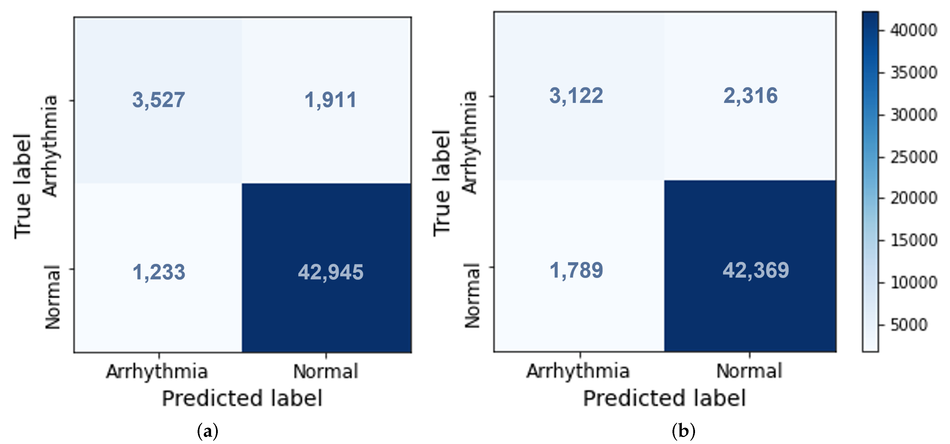
Besides these, the receiver operating characteristic (ROC) curve and the confusion matrix were used to assess the quality of the classification. The ROC curve plots the true positive rate over the false positive rate and shows how well a model can distinguish between two classes. The confusion matrix is illustrated in Figure 1, and illustrates the number of TP, FP, TN, and true negative (TN) graphically.
Each model was trained in a computer with 2 NVIDIA Geforce RTX 2080 8GB GPUs with 64 GB of RAM and a i7-9700K 3.6 GHz CPU.

3.3. Explainability Methods

We used three different explainability methods: gradients (generates saliency maps), grad-CAM, and guided backpropagation grad-CAM. Besides being local and post hoc methods, they are also backpropagation-based methods. According to [28], backpropagation-based methods compute attribution for all input features with a single forward and backward pass through the network. Some methods inside this category can only provide positive contributions to the final prediction result in the attribution map, while others show the positive and negative contributions, which may degrade the results by increasing the noise in the map.

3.3.1. Gradients Method

The gradients method originates saliency maps and is the earliest and probably one of the most used methods to explain the predictions of CNNs. The saliency map of the input of a CNN highlights the parts of the input that most contributes to the outcome and, so, the method attributes importance to each pixel of an input image regarding the prediction of the network.
Based on the work that introduced this method, the pixel importance is obtained by applying the somewhat inverse operation relative to the training of neural networks (NN) [29]. Neural networks are usually trained by the application of backpropagation regarding the expected labels to optimise the loss function. The backpropagation method is applied from the input to the output of the networks. However, to obtain the saliency maps, the same backpropagation algorithm is applied, but in this case the derivative is applied regarding the input image (Equation (4)):
w = y c I | I 0
where y c is the class score, I is the image, and I 0 is the input image, specific for the task at hand, and w is the attribution map—analogous to the weights of NN.

3.3.2. Gradient-Weighted Class Activation Mapping

Gradient-weighted class activation mapping (grad-CAM) was first introduced in [30] as a generalisation of class activation mapping (CAM). Unlike CAM, grad-CAM can be used to visualise any type of CNNs. Grad-CAM uses gradient information that flows to the last convolution layer to compute the importance, for the prediction, of each neuron. The last convolutional layers of a CNN retain spatial information and its neurons are focused on semantic class-specific information in the input image. For this reason, grad-CAM is a class discriminative method.
Equation (5) shows how to compute the weight α k c . This weight captures the importance of a feature map k for a target class c. This value is the global average pooling of the gradient of the score (before softmax) for class, c, w.r.t the feature maps, A k : y c A i j k :
α k c = 1 Z i j y c A i j k .
After this step, a weighted combination of forward activation maps and a ReLU are necessary to compute the final map, as shown in Equation (6). The application of the ReLU guarantees that the attribution map only depicts the positive contributions to the classification result:
L Grad CAM c = ReLU k α k c A k .
These operations create a coarse heat map of the same size as the convolutional feature maps. Although we can apply grad-CAM to any convolutional layer, as we are trying to explain the decisions of our classifier, we applied the method to the last convolutional layer of our ResNet.

3.3.3. Guided Backpropagation Gradient-Weighted Class Activation Mapping

The guided backpropagation grad-CAM (GB grad-CAM) was also introduced in [30]. This method was developed to tackle the lack of finer details in the attribution maps created using grad-CAM. GB grad-CAM consists of a pixel-wise multiplication between a grad-CAM map and guided backpropagation (GB) map.
GB maps were first described in [31]. These maps are an improved version of the saliency maps. Instead of using a normal backpropagation approach, they use a guided backpropagation. GB combines two methods: ‘Deconvnet’ [32] and backpropagation. These methods differ only in the way they handle backpropagation through the ReLU nonlinearity. The ‘deconvnet’ method, considers only the top gradient signal to compute the gradient in the nonlinearity and ignores the bottom input. GB combines this with backpropagation and masks out the values for which the top gradient or bottom data are negative. This prevents the backward flow of negative gradients.

3.4. Quantitative Analysis of Pixel Attribution Maps

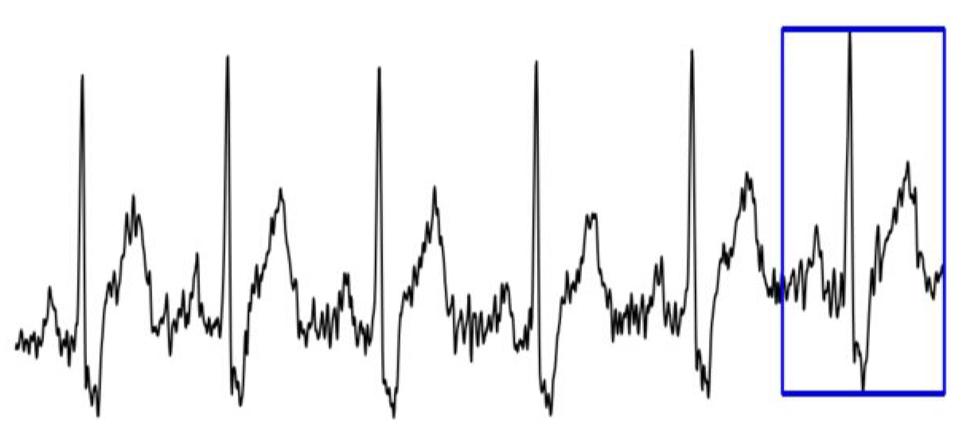
We computed a proportion of attribution between the heartbeat of interest and the rest of the image to study the magnitude of focus in the different regions of the ECG images. Firstly, we computed a rectangular region of interest (ROI) that contains only the heartbeat of interest. This heartbeat is the labelled heartbeat that varies according to the dataset. Figure 2 illustrates an example of a computed ROI. In that case, the last beat was the heartbeat of interest. Then, we determine the proportion between the total sum of the pixel attribution map and the sum of the map inside the region of interest. Using this proportion we are able to measure the percentage of focus inside the ROI.

4. Results

This work can be divided in two distinct parts: One regarding the classification of ECG images and the other focused on the analysis of the created attribution maps using our custom metric.

4.1. Classification

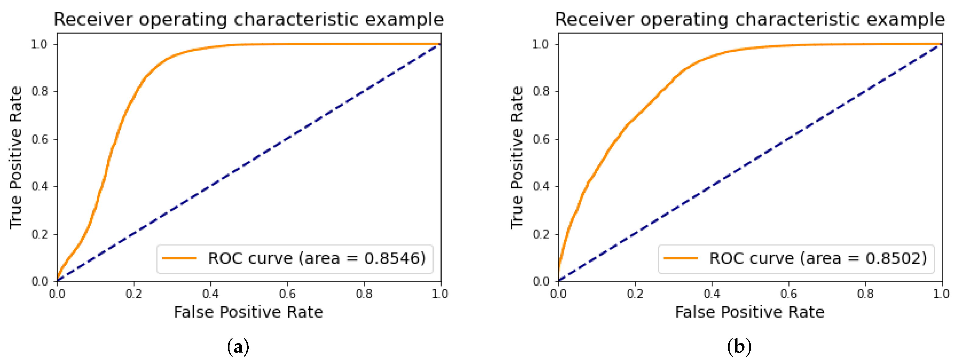
Table 1 presents the number of epochs and training time, the values of accuracy and F 1 -score computed in the validation and test set, and the precision score computed only at the testing stage. Figure 3 and Figure 4 are related with the testing stage of our models. Figure 3 presents the confusion matrix of each model. Figure 4 presents the receiver operating characteristic (ROC) curve and the area under the curve (AUC) of the ROC. In a brief analysis, we can conclude that model 1 (label corresponding to the last heartbeat of the figure) performs better in terms of global accuracy than model 2 (label corresponding to the first heartbeat of the ECG figure) in the testing set, with an accuracy of 93.66%. However both the confusion matrices and the AUC values are very similar for each model Table 1.

4.2. Explainability Metric

Regarding the explored explainability metric, we present three different scenarios.

4.2.1. Generic Scenario

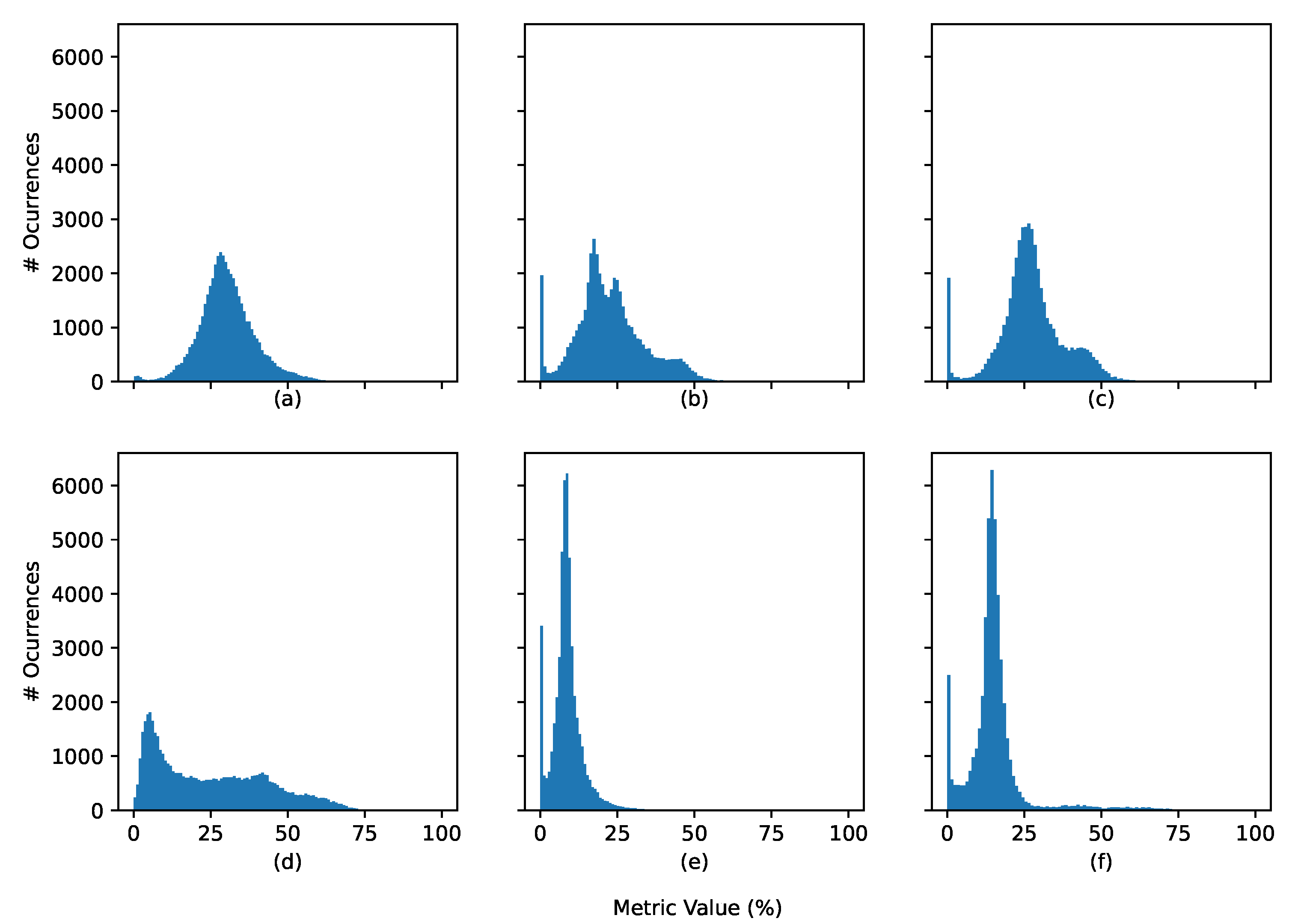
The generic scenario, presented in Table 2 and the histograms shown in Figure 5, is the overall comparison of the three explainability methods relative to the classification of the two models. In this case, we see that the method that better focuses the heartbeat of interest in both classification models is the gradients method, with a focus of around 30% in model 1 and 25% in model 2, while the Grad-CAM is the method with the worst focus with a focus of around 23% in model 1 and 9% in model 2. The comparison between the two models revealed a value p < 0.001 for the null hypothesis that the mean values for each explainability method are equal. A t-test for the means of two independent samples distribution was used.

4.2.2. Correct vs. Incorrect Classification

The comparison between correct classification and incorrect classification, presented in Table 3, shows that in the case of the Grad-CAM and GB grad-CAM in model 1, there is a positive relation between correct classification and the focus of the attribution maps. Notwithstanding, in model 2 there is not a clear relation between the classification results and the focus of the attribution maps. The comparison between the two models revealed a value p < 0.001 for the null hypothesis and that the mean values for each correct vs. incorrect comparison of each explainability method are equal. Moreover, the value p for the comparison between sets is lower than 0.001 between all cases, aside from the wrong vs. wrong case using the saliency maps and the GB grad-CAM maps. A t-test for the means of two independent samples distribution was used.

4.2.3. Normal vs. Arrhythmia

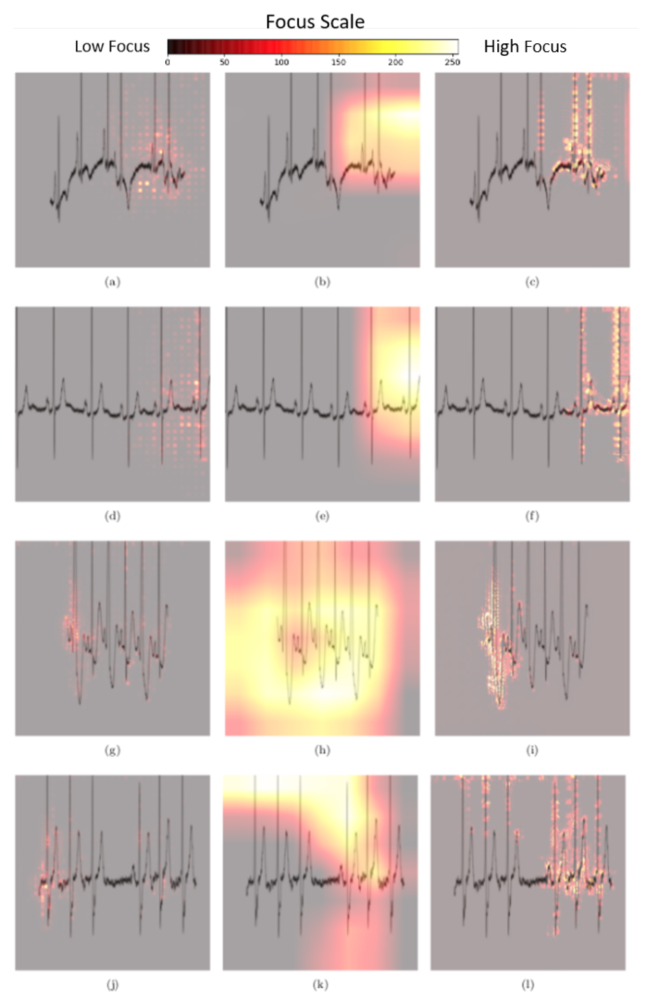
Finally, the comparison between the two labels of the images, presented in Table 4 and exemplified in Figure 6, shows that there is not a consistent relation between the label of the images and the focus of the attribution maps. For example, the Grad-CAM shows better results in model 1 for the normal label, while for model 2 the opposite happens. The comparison between the two models revealed a value p < 0.001 for the null hypothesis that the mean values for each normal vs. arrhythmia comparison of each explainability method are equal. Moreover, the value p for the comparison between sets is lower than 0.001 between all cases. A t-test for the means of two independent samples distribution was used.

5. Discussion

The first step in our project was to detect arrhythmia in the last or first heartbeat within ECG images containing six heartbeats. Thus, we created two different models: One to classify the last heartbeat (model 1) and another to classify the first heartbeat (model 2). Table 1 shows that model 1 performs slightly better than model 2 at the testing set, consisting of patients that are not in the other sets (interpatient classification). We hypothesise that, similarly to how humans classify ECG, the beats prior to the heartbeat of interest help the model to produce the correct prediction.
During training, the low number of epochs and the difference of the number of epochs between the two models is also noticeable. This difference is related to how the stopping criteria of the early stop mechanism was implemented. Training stopped after 4 epochs of decreasing F 1 -score and, thus, if the criteria was different, the number of epochs might have been higher or lower. However, the fact that the training epochs of each model is different does not influence their results, since the stopping criteria was the same. Thus, even if both models continued training, the F 1 -score would not increase.
The confusion matrices show that our classification models struggle to correctly identify the positive label as reflected by the low precision scores (74.10 % and 63.57%) and proximity between the values of false and true positives. However, the AUC-ROC value shows a 85% probability of distinguishing between the positive and negative label. Our classification accuracy scores of 91–94% were slightly below the state of the art results presented in [13,14,15,16]. When comparing with studies [18,19,20] that used ECG as an image we also concluded that our classification results were inferior. However we cannot perform a direct comparison because those studies were not clear regarding if they performed patient division across the data sets. The inferior results can be explained by multiple factors. We use the ECG signal of only one lead of the MIT BIH database without any pre-processing. This can be problematic because some ECG signals in that database have a low signal-to-noise ratio, even after removing the intractable parts of signals. In addition, some arrhythmia events are not visible in all leads. Finally, we used the dataset division proposed in [10], but samples from the training set were used to build the validation set, resulting in a testing set that was larger than the training set. By doing this, we are certain to use the same testing set as most of the reported studies. Since our main objective was the transparency of DL models, we did not focus on the optimisation of the classification results.
After the classification task, the next step was the application of the already enumerated explainability methods to create attribution maps. From those maps we computed our metric to measure the amount of focus of the model on the heartbeat of interest. The maps created using the gradients method do not distinguish between positive or negative contributions to the model prediction [28]. Attribution maps created using grad-CAM and GB grad-CAM methods only consider positive contributions. For this reason, the values of our metric are generally higher for attributions maps created using the gradients method. Nevertheless, we expect the model to focus on the region of the labelled heartbeat, even if certain pixels of that region give negative contributions to the prediction.
Supposing that the model is not focused in any particular area of the input images, the average value of our metric would be 9.7 ± 4.0 % . We called this value the random focus value. This value was estimated by computing the average proportion between the area of the region of interest and the area of the image across all test samples. The values shown in Table 2, Table 3 and Table 4 are higher than the random focus value for all attribution maps except for specific cases in the grad-CAM attribution maps. This fact implies that both our models considered the region of the labelled heartbeat an important region to the prediction process. For further analysis we created three different scenarios for comparison: The generic case; the correct vs. incorrect classification case; and the abnormal vs. normal label case.
From the generic case, we can conclude that the obtained values of the attribution metric corroborate the better classification performance of model 1. Model 1 has higher values for all maps. From Table 2, we can also highlight the fact that the attribution metric using grad-CAM in model 2 was the only one below the random focus value. In fact, generally, grad-CAM had the lowest values for all cases. Grad-CAM maps are the most coarse attribution maps of the three different maps that were created [33]. Therefore the higher pixel values are more scattered across the map, when comparing with the other maps, resulting in lower values of our custom attribution metric. The histograms presented in Figure 5 show that despite having the higher average values, model 1 also has higher deviation values for all maps, except for the ones created using gradients method—(a) and (d). The frequency of null values can also be seen as not negligible for the grad-CAM and GB grad-CAM methods—(b), (e) and (c), (f). Those null values represent the cases where there is no pixel attribution of positive contributions inside the region of interest. Gradients maps have a negligible frequency of null values because they consider positive and negative contributions to the prediction process.
With the second scenario, Table 3, we extrapolate a relation between the value of our custom attribution metric and the coherence between the classification result and the actual label of the samples. We expected that correct classifications to be related with a more focused model (higher values of the metric) however this is not the case when applying the gradients method. This is again related to the nature of the method, which does not distinguish between positive and negative contributions.
Finally, our third scenario, Table 4, focuses on the relation between the actual label of the test sample and its attribution map. Here we cannot find a general tendency for both models. For model 1, both GB grad-CAM and grad-CAM have higher values when classifying normal samples. On the contrary for model 2, higher values are obtained when classifying abnormal samples. Gradients maps have higher values for abnormal samples in both models. These tendencies can be seen in Figure 6.
Notwithstanding that we are assessing the focus of our classification model in the region that contains the labelled heartbeat, we also hypothesise that high attribution values outside that region in our input images might be relevant for classification. There, the focus can be on the blank parts of the figures or in the remaining heartbeats that do not contribute to the label. In the first case, the model might be searching for heartbeats that should happen (e.g., if the signal is shorter than expected) or for higher amplitude signals than the ones that are present. In the second case, the model might be looking for inter-beat features, such as, the distance between R peaks, to classify the most important beat (important in some arrhythmia cases, such as tachycardia or bradycardia). In fact, the low values of our metric support this hypothesis, but further research is required for validation.
In its present condition our work cannot be applied in clinical settings. First of all, the accuracy and precision scores are not high enough. The fact that there are numerous false negatives could lead to serious misdiagnosis. On the other hand, the explainability still needs improvement, as previously mentioned. Namely, the focused region should be contained on the sites of the abnormality and, in this case, the focus is still somewhat sparse across the figures. However, our explainability metric might allow future works to quantitatively assess the quality of their explainability methods. Ideally, all focus should be on the ROI and the ROI should be clearly identified.

6. Conclusions

In this study, we built two computer vision classification models and applied three different backpropagation-based explainability methods to each to create attribution maps. From the attribution maps, we then created a custom metric that measures the degree of importance of each pixel of the input image given the classification result. Then, we compared the obtained values of our metric across different cases: The generic case, accurate vs. inaccurate classification, and abnormal vs. normal samples.
Our classification results were below the state of the art results. Both models achieved testing accuracy scores between 91–94%. The values of our metric ranged between 8 and 38% with high standard deviation values. Those values show that the focus of the classification models is sparse across the ECG image, even though there is a concentration of focus in the heartbeat of interest.
For future work, we will improve the classification results by pre-processing the ECG signals. Moreover, we will improve the computation of the heartbeat region of interest to be more precise. We will extend the knowledge on this subject by analysing the importance of other regions of the ECG images. We will explore specific waves inside of the heartbeat of interest to assess their importance to classification (e.g., P and T waves, and QRS complex). Furthermore, it would be interesting to explore if DL models capture pseudo-time dependencies by computing the distant between R peaks and other commonly extracted features, which might explain the importance of regions of interest besides the labelled heartbeat.

Author Contributions

Conceptualisation, R.V. and B.G.; methodology, R.V. and B.G.; software, R.V. and B.G.; validation, H.G. and P.V.; investigation, R.V. and B.G.; data curation, R.V. and B.G.; writing—original draft preparation, R.V. and B.G.; writing—review and editing, R.V., B.G., H.G. and P.V.; visualisation, R.V. and B.G.; supervision, H.G. and P.V. All authors have read and agreed to the published version of the manuscript.

Funding

This work was funded by FCT—Portuguese Foundation for Science and Technology and Bee2Fire under the PhD grant with reference PD/BDE/150624/2020. Moreover, it was funded by FCT—Portuguese Foundation for Science and Technology and PLUX Wireless Biosignals S.A. under the PhD grant with reference PD/BDE/150304/2019.

Institutional Review Board Statement

Not applicable.

Informed Consent Statement

Not applicable.

Data Availability Statement

The raw data used in this work is publicly available at https://physionet.org/content/mitdb/1.0.0/ (accessed on 7 January 2022). The transformed data can be found in [34].

Acknowledgments

We would like to acknowledge André Martins from the Instituto Superior Técnico, Universidade de Lisboa, for his input in the early stages of this work.

Conflicts of Interest

The authors declare no conflict of interest.

References

  1. Vellido, A. Societal Issues Concerning the Application of Artificial Intelligence in Medicine. Kidney Dis. 2019, 5, 11–17. [Google Scholar] [CrossRef] [PubMed]
  2. Liang, Y.; Li, S.; Yan, C.; Li, M.; Jiang, C. Explaining the black-box model: A survey of local interpretation methods for deep neural networks. Neurocomputing 2021, 419, 168–182. [Google Scholar] [CrossRef]
  3. Hamon, R.; Junklewitz, H.; Sanchez, I. Robustness and Explainability of Artificial Intelligence; Publications Office of the European Union: Luxembourg, 2020; p. 40. [Google Scholar] [CrossRef]
  4. Rudin, C. Stop explaining black box machine learning models for high stakes decisions and use interpretable models instead. Nat. Mach. Intell. 2019, 1, 206–215. [Google Scholar] [CrossRef] [Green Version]
  5. Molnar, C. Interpretable Machine Learning. 2019. Available online: https://christophm.github.io/interpretable-ml-book/ (accessed on 10 January 2022).
  6. Linardatos, P.; Papastefanopoulos, V.; Kotsiantis, S. Explainable ai: A review of machine learning interpretability methods. Entropy 2021, 23, 18. [Google Scholar] [CrossRef]
  7. Ploug, T.; Holm, S. The four dimensions of contestable AI diagnostics—A patient-centric approach to explainable AI. Artif. Intell. Med. 2020, 107, 101901. [Google Scholar] [CrossRef]
  8. Chapter 3—Rights of the Data Subject|General Data Protection Regulation (GDPR). General Data Protection Regulation (GDPR). 2018. Available online: https://gdpr-info.eu/chapter-3/ (accessed on 14 June 2021).
  9. Clarke, N.; Vale, G.; Reeves, E.P.; Kirwan, M.; Smith, D.; Farrell, M.; Hurl, G.; McElvaney, N.G. GDPR: An impediment to research? Ir. J. Med Sci. 2019, 188, 1129–1135. [Google Scholar] [CrossRef] [Green Version]
  10. Luz, E.J.d.S.; Schwartz, W.R.; Cámara-Chávez, G.; Menotti, D. ECG-based heartbeat classification for arrhythmia detection: A survey. Comput. Methods Programs Biomed. 2016, 127, 144–164. [Google Scholar] [CrossRef]
  11. Luz, E.J.D.S.; Nunes, T.M.; De Albuquerque, V.H.C.; Papa, J.P.; Menotti, D. ECG arrhythmia classification based on optimum-path forest. Expert Syst. Appl. 2013, 40, 3561–3573. [Google Scholar] [CrossRef] [Green Version]
  12. Dong, X.; Wang, C.; Si, W. ECG beat classification via deterministic learning. Neurocomputing 2017, 240, 1–12. [Google Scholar] [CrossRef]
  13. Pyakillya, B.; Kazachenko, N.; Mikhailovsky, N. Deep Learning for ECG Classification. J. Phys. Conf. Ser. 2017, 913, 012004. [Google Scholar] [CrossRef]
  14. Rim, B.; Sung, N.J.; Min, S.; Hong, M. Deep learning in physiological signal data: A survey. Sensors 2020, 20, 969. [Google Scholar] [CrossRef] [PubMed] [Green Version]
  15. Somani, S.; Russak, A.J.; Richter, F.; Zhao, S.; Vaid, A.; Chaudhry, F.; Freitas, J.K.D.; Naik, N.; Miotto, R.; Nadkarni, G.N.; et al. Deep learning and the electrocardiogram: Review of the current state-of-the-art. Europace 2021, 23, 1179–1191. [Google Scholar] [CrossRef]
  16. Ebrahimi, Z.; Loni, M.; Daneshtalab, M.; Gharehbaghi, A. A review on deep learning methods for ECG arrhythmia classification. Expert Syst. Appl. X 2020, 7, 100033. [Google Scholar] [CrossRef]
  17. Rahhal, M.M.; Bazi, Y.; Alhichri, H.; Alajlan, N.; Melgani, F.; Yager, R.R. Deep learning approach for active classification of electrocardiogram signals. Inf. Sci. 2016, 345, 340–354. [Google Scholar] [CrossRef]
  18. Degirmenci, M.; Ozdemir, M.A.; Izci, E.; Akan, A. Arrhythmic Heartbeat Classification Using 2D Convolutional Neural Networks. IRBM 2021. [Google Scholar] [CrossRef]
  19. Naz, M.; Shah, J.H.; Khan, M.A.; Sharif, M.; Raza, M.; Damaševičius, R. From ECG signals to images: A transformation based approach for deep learning. PeerJ Comput. Sci. 2021, 7, e386. [Google Scholar] [CrossRef]
  20. Franklin, R.G.; Muthukumar, B. Arrhythmia and Disease Classification Based on Deep Learning Techniques. Intell. Autom. Soft Comput. 2021, 31, 835–851. [Google Scholar] [CrossRef]
  21. Mousavi, S.; Afghah, F.; Acharya, U.R. HAN-ECG: An interpretable atrial fibrillation detection model using hierarchical attention networks. Comput. Biol. Med. 2020, 127, 104057. [Google Scholar] [CrossRef] [PubMed]
  22. Maweu, B.M.; Dakshit, S.; Shamsuddin, R.; Prabhakaran, B. CEFEs: A CNN Explainable Framework for ECG Signals. Artif. Intell. Med. 2021, 115, 102059. [Google Scholar] [CrossRef]
  23. Jo, Y.Y.; Kwon, J.M.; Jeon, K.H.; Cho, Y.H.; Shin, J.H.; Lee, Y.J.; Jung, M.S.; Ban, J.H.; Kim, K.H.; Lee, S.Y.; et al. Detection and classification of arrhythmia using an explainable deep learning model. J. Electrocardiol. 2021, 67, 124–132. [Google Scholar] [CrossRef] [PubMed]
  24. Yoo, J.; Jun, T.J.; Kim, Y.H. xECGNet: Fine-tuning attention map within convolutional neural network to improve detection and explainability of concurrent cardiac arrhythmias. Comput. Methods Programs Biomed. 2021, 208, 106281. [Google Scholar] [CrossRef] [PubMed]
  25. Moody, G.B.; Mark, R.G. The impact of the MIT-BIH arrhythmia database. IEEE Eng. Med. Biol. Mag. 2001, 20, 45–50. [Google Scholar] [CrossRef] [PubMed]
  26. He, K.; Zhang, X.; Ren, S.; Sun, J. Deep residual learning for image recognition. In Proceedings of the IEEE Computer Society Conference on Computer Vision and Pattern Recognition, Las Vegas, NV, USA, 27–30 June 2016; pp. 770–778. [Google Scholar] [CrossRef] [Green Version]
  27. Deng, J.; Dong, W.; Socher, R.; Li, L.J.; Li, K.; Li, F. Imagenet: A large-scale hierarchical image database. In Proceedings of the 2009 IEEE Conference on Computer Vision and Pattern Recognition, Miami, FL, USA, 20–25 June 2009; pp. 248–255. [Google Scholar]
  28. Singh, A.; Sengupta, S.; Lakshminarayanan, V. Explainable deep learning models in medical image analysis. J. Imaging 2020, 6, 52. [Google Scholar] [CrossRef]
  29. Simonyan, K.; Vedaldi, A.; Zisserman, A. Deep Inside Convolutional Networks: Visualising Image Classification Models and Saliency Maps. arXiv 2014, arXiv:1312.6034. [Google Scholar]
  30. Selvaraju, R.R.; Cogswell, M.; Das, A.; Vedantam, R.; Parikh, D.; Batra, D. Grad-CAM: Visual Explanations from Deep Networks via Gradient-Based Localization. In Proceedings of the 2017 IEEE International Conference on Computer Vision (ICCV), Venice, Italy, 22–29 October 2017; pp. 618–626. [Google Scholar] [CrossRef] [Green Version]
  31. Springenberg, J.T.; Dosovitskiy, A.; Brox, T.; Riedmiller, M. Striving for simplicity: The all convolutional net. In Proceedings of the 3rd International Conference on Learning Representations, ICLR 2015—Workshop Track Proceedings, San Diego, CA, USA, 7–9 May 2015; pp. 1–14. [Google Scholar]
  32. Zeiler, M.D.; Fergus, R. Visualizing and Understanding Convolutional Networks. In Analytical Chemistry Research; Springer: Cham, Switzerland, 2014; Volume 12, pp. 818–833. [Google Scholar] [CrossRef] [Green Version]
  33. Selvaraju, R.R.; Cogswell, M.; Das, A.; Vedantam, R.; Parikh, D.; Batra, D. Grad-cam: Why did you say that? visual explanations from deep networks via gradient-based localization. Rev. Hosp. Clin. 2016, 17, 331–336. [Google Scholar]
  34. Varandas, R.; Gonçalves, B. Quantified Explainability: Convolutional Neural Network Focus Assessment in Arrhythmia Detection. Res. Sq. 2022. [Google Scholar] [CrossRef]
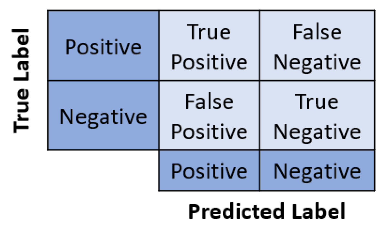
Figure 1. Confusion matrix representation.
Biomedinformatics 02 00008 g001
Figure 2. Normal electrocardiographic signal with a rectangular region of interest (ROI) that contains the last heartbeat.
Biomedinformatics 02 00008 g002
Figure 3. Confusion matrices of the models at testing stage. Arrhythmia—positive label. Normal—negative label. (a) Model 1. (b) Model 2.
Biomedinformatics 02 00008 g003
Figure 4. Receiving Operating Characteristic (ROC) curves and Area Under the Curve (AUC) values of the models at testing stage. (a) Model 1. (b) Model 2.
Biomedinformatics 02 00008 g004
Figure 5. Histograms of the distribution of the custom attribution metric values for the generic case. (ac) correspond to the metrics estimated using model 1 and the methods: Gradients, grad-CAM, and GB grad-CAM, respectively. (df) correspond to the metrics estimated using model 2 and the methods: Gradients, grad-CAM, and GB grad-CAM, respectively.
Biomedinformatics 02 00008 g005
Figure 6. Examples from the obtained attribution maps. The first row of figures corresponds to maps created using model 1 (the heartbeat of interest is the last) and to an abnormal sample: (a) Saliency map; (b) grad-CAM map; and (c) GB grad-CAM map. The second row corresponds to maps created using model 1 and to a normal sample: (d) Saliency map; (e) grad-CAM map; and (f) GB grad-CAM map. The third row corresponds to maps created using model 2 (the heartbeat of interest is the first) and to an abnormal sample: (g) Saliency map; (h) grad-CAM map; and (i) GB grad-CAM map. The fourth row corresponds to maps created using model 2 and a normal sample: (j) Saliency map; (k) grad-CAM map; and (l) GB grad-CAM map. In all the presented cases, the models gave the correct predictions. The scale presented at the top implies that the brighter pixels correspond to a higher focus.
Biomedinformatics 02 00008 g006
Table 1. Classification metrics. The models 1, 2, were trained with dataset 1, 2, respectively. The presented values are percentages, except for the train time and number of epochs.
ModelsTrainValidationTest
TimeEpochsAccuracyF 1 -ScoreAccuracyF 1 -ScorePrecision
Model 142 min794.0696.8293.6696.4774.10
Model 233 min596.2398.0091.7295.3863.57
Table 2. Attribution metric—generic. Mean value ± standard deviation value of the metric of all test samples. Each line for a different dataset: 1—last heartbeat labelled; 2—first heartbeat labelled. All presented values are percentages.
SetGradientsGrad-CAMGB Grad-CAM
1 30.3 ± 9.2 22.7 ± 11.5 27.4 ± 10.9
2 25.0 ± 18.2 8.7 ± 5.2 15.3 ± 9.9
Table 3. Attribution metric—correct classification vs. incorrect classification. Mean value ± standard deviation value of the metric of the test samples according to their accuracy of classification. Each line for a different dataset: 1—label corresponding to the last heartbeat; 2—label corresponding to the first heartbeat. All presented values are percentages.
SetGradientsGrad-CAMGB Grad-CAM
CorrectIncorrectCorrectIncorrectCorrectIncorrect
1 30.3 ± 8.9 31.4 ± 12.6 23.6 ± 10.7 10.2 ± 15.2 28.3 ± 9.7 13.3 ± 16.8
2 24.4 ± 18.0 32.4 ± 19.3 8.8 ± 4.3 8.3 ± 10.8 15.5 ± 8.8 12.7 ± 19.4
Table 4. Attribution metric—abnormal label vs. normal label. Mean value ± standard deviation value of the metric of the test samples that are abnormal and those which are normal. Each line for a different dataset: 1—last heartbeat labelled; 2—first heartbeat labelled. All presented values are percentages.
SetGradientsGrad-CAMGB Grad-CAM
AbnormalNormalAbnormalNormalAbnormalNormal
1 34.6 ± 10.3 29.8 ± 8.9 18.4 ± 15.5 23.3 ± 10.8 24.0 ± 17.9 27.8 ± 9.7
2 39.7 ± 19.3 23.2 ± 17.3 10.7 ± 10.2 8.5 ± 4.2 31.9 ± 24.1 13.8 ± 5.2
Publisher’s Note: MDPI stays neutral with regard to jurisdictional claims in published maps and institutional affiliations.