Explainable Machine Learning (XAI) for Survival in Bone Marrow Transplantation Trials: A Technical Report

Abstract

Artificial intelligence is gaining interest among clinicians, but its results are difficult to be interpreted, especially when dealing with survival outcomes and censored observations. Explainable machine learning (XAI) has been recently extended to this context to improve explainability, interpretability and transparency for modeling results. A cohort of 231 patients undergoing an allogeneic bone marrow transplantation was analyzed by XAI for survival by two different uni- and multi-variate survival models, proportional hazard regression and random survival forest, having as the main outcome the overall survival (OS) and its main determinants, using the survex package for R. Both models’ performances were investigated using the integrated Brier score, the integrated Cumulative/Dynamic AUC and the concordance C-index. Global explanation for the whole cohort was performed using the time-dependent variable importance and the partial dependence survival plot. The local explanation for each single patient was obtained via the SurvSHAP(t) and SurvLIME plots and the ceteris paribus survival profile. The survex package common interface ensured a good feasibility of XAI for survival, and the advanced graphical options allowed us to easily explore, explain and compare OS results coming from the two survival models. Before the modeling results to be suitable for clinical use, understandability, clinical relevance and computational efficiency were the most important criteria ensured by this XAI for survival approach, in adherence to clinical XAI guidelines.

1. Introduction

Machine learning (ML) techniques are gaining an increased interest among cancer clinicians, mainly due to the availability of classification algorithms for automatic computer-assisted diagnosis [1]. At the same time, these techniques need to be deeply adapted to censored observations and time-to-event outcomes like overall survival (OS), a classical endpoint in oncohematology and allogeneic bone marrow transplantation (BMT) trials [2,3,4]. Actually, survival ML modeling is still limited not only by the availability of dedicated algorithms and software, but even more so by the critical interpretation of its results. In the last years, several explainable machine learning (XAI) algorithms have been introduced by different authors, stating three main principles: XAI should improve explainability, interpretability and transparency for ML modeling results. The XAI algorithms’ goal is then to convert “black-box” dark ML predictions into more interpretable “white-box” glass ones; doing so, physicians could more easily translate the complex information deriving from ML models into reliable, daily clinical choices [5,6,7,8,9]. Very recently, the XAI approach has been extended to survival models too [10,11,12]. This study aims to test this approach in a real-world evidence context, estimating the OS and its determinants for a cohort of patients undergoing allogeneic BMT, using two different survival models: the Cox proportional hazard regression model (PH) and the random survival forest [13,14].

2. Materials and Methods

The clinical trial took place at the Stem Cell Transplantation Center of the Città della Salute e della Scienza Hospital of Torino-I and enrolled 231 patients from 2008 to 2021, receiving an allogeneic stem cell transplantation from unrelated donors (MUD) and all being treated with a fixed dose (5 mg/kg) of anti-thymocyte globulin (ATG) as Graft-versus-Host Disease (GVHD) prophylaxis [15]. Acute and chronic GvHD, as well treatment-related adverse events and systemic infections, are the most severe toxicities after BMT, being the main causes of death for relapse-free patients (NRM, Non Relapse Mortality). This research is a reanalysis of the original dataset, in light of the recent scenario opened by the introduction of XAI for survival; clinical history and treatment decisions for all patients have not been changed following the current results. Due to the retrospective observational nature of this trial and according to Italian law (Agenzia Italiana del Farmaco-AIFA, Guidelines for observational studies, 20 March 2008), no formal approval from the local Institutional Review Board/Independent Ethics Committee was needed.

Statistical Analysis

The primary outcome was the OS, defined as the time from BMT to death from any cause/last follow-up; the median follow-up for the surviving subjects was 56 (IQR 30–81) months. The OS was analyzed using either the proportional hazards regression model (coxph) or the random survival forest (rfsrc), using XAI for survival to explore and explain their results.

From the pool of the original study dataset (consisting of 18 covariates,

Table 1. Main patients’ characteristics of the whole cohort.

Characteristics	All Patients
Age at transplant, median (IQR), years	51 (43–60)
Gender
Male	126 (54.5%)
Female	105 (45.5%)
HCT-CI
Low/intermediate (0–2)	119 (68.4%)
High (>3)	55 (31.6%)
Cytogenetics
Low risk	53 (35.6%)
Intermediate/High risk	96 (64.4%)
CMV Recipient status
negative	67 (30.3%)
positive	154 (69.7%)
Conditioning regimen
MAC	199 (86.1%)
RIC	32 (13.9%)
Year of transplant
2008–2012	47 (20.3%)
2013–2017	98 (42.4%)
2018–2021	86 (37.3%)
Chronic GvHD
absent/mild	131 (68.6%)
moderate/severe	60 (31.4%)
Overall Survival
alive	133 (57.6%)
dead	98 (42.4%)

Abbreviations: HCT-CI hematopoietic cell transplantation-comorbidity index, CMV cytomegalovirus, IQR inter quartile range, MAC myeloablative conditioning, RIC reduced intensity conditioning, GvHD graft versus host disease.

), we selected eight for the current research: those being statistically significant predictors at the original multivariate OS Cox PH model. These eight features were tested as potential OS risk factors: recipient age (≥60 vs. 40–60 vs. <40 years), recipient gender (male vs. female), cytogenetic risk (intermediate/high vs. low), recipient CMV status (positive vs. negative), Sorror Comorbidity Index (HCT-CI, ≥3 vs. 0–2), conditioning regimen (reduced intensity (RIC) vs. myeloablative (MAC)), chronic GVHD (moderate/severe vs. no/mild) occurrence and year of BMT (2018–2021 vs. 2013–2017 vs. 2008–2012). At first, missing values were replaced using the Multiple Imputation by Chained Equations procedure: cytogenetic risk was unknown for 82 subjects, HCT-CI for 57 and recipient CMV status for 10, while the other five covariates had no missing values.

For both approaches (coxph and rfsrc), model performance was investigated using the integrated Brier score, the integrated Cumulative/Dynamic AUC and the concordance C-index. Global explanation for the whole cohort was then performed using the time-dependent variable importance and the partial dependence survival plot. Finally, the local explanation for a single statistical unit (that is to say, a single patient) was obtained from the SurvSHAP(t) and SurvLIME plots and the ceteris paribus survival profile. In all graphics, the x-axis reported the time from BMT to death from any cause/last follow-up; event times are marked in red, censor times in grey.

Patient characteristics were estimated using the Fisher’s exact test for the categorical variables and the Mann–Whitney test for the continuous ones, reporting them as median [interquartile range (IQR)]. All p-values were obtained using the two-sided exact method, at the conventional 5% significance level. Data were analyzed as of June 2023 by R 4.3.0, survex, randomForestSRC and mice packages (R Foundation for Statistical Computing, Vienna-A, http://www.R-project.org, accessed on 15 August 2023).

3. Results

The results of XAI for survival using the survex R package have to follow a dedicated and specific workflow, as reported in the diagram. The first step implies a model performance estimation, both for coxph and rfsrc. In case of acceptable results, it is possible to move on at the second step, using XAI for survival to explain the OS estimation for the whole cohort (231 subjects). The third and final step allows for a reply to the OS estimation process for each single patient: this is a notable advantage, comparing to the classical survival modeling.

1—Model performance for the whole cohort

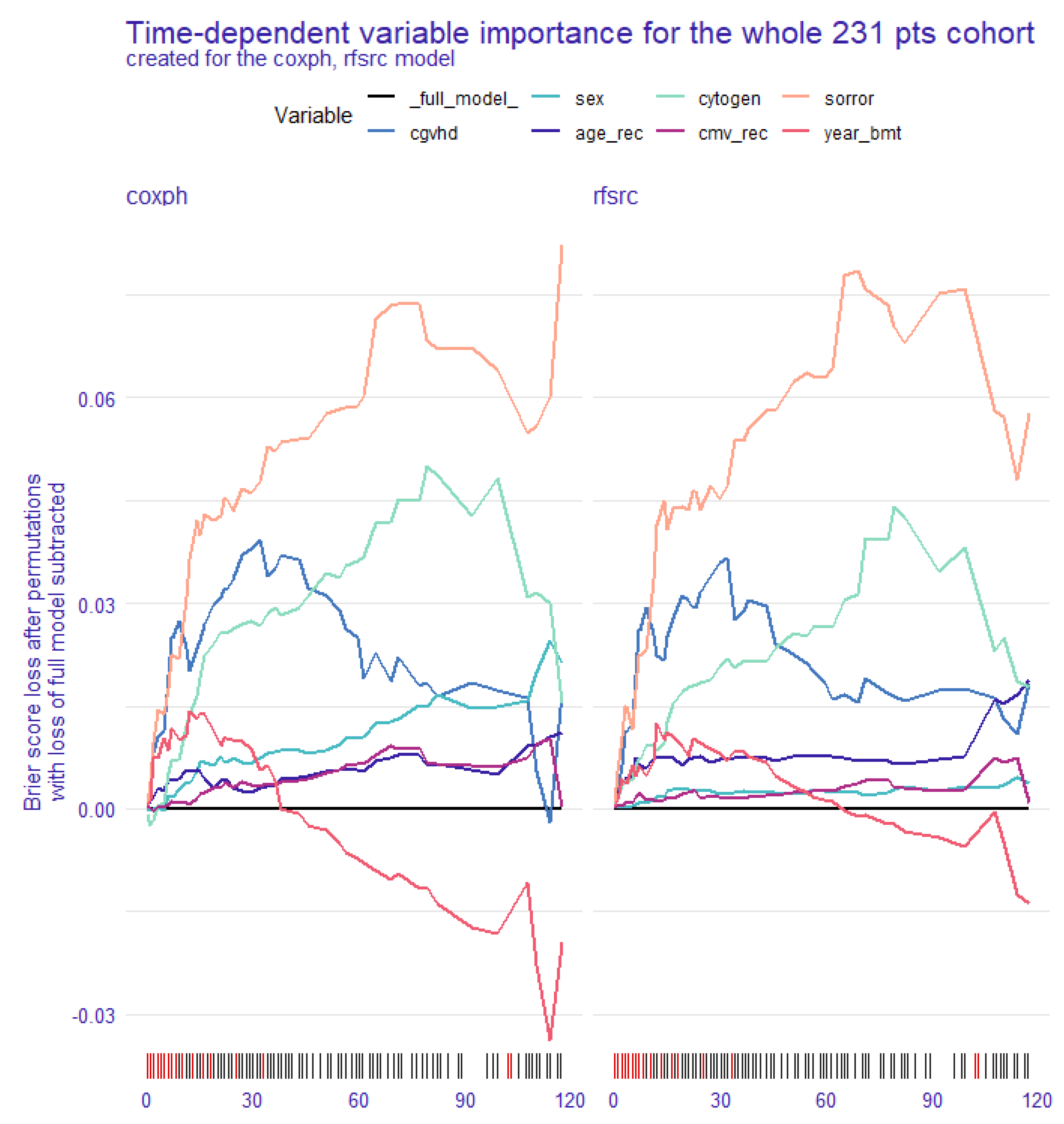
2a—Global explanation: time-dependent feature importance for the whole cohort

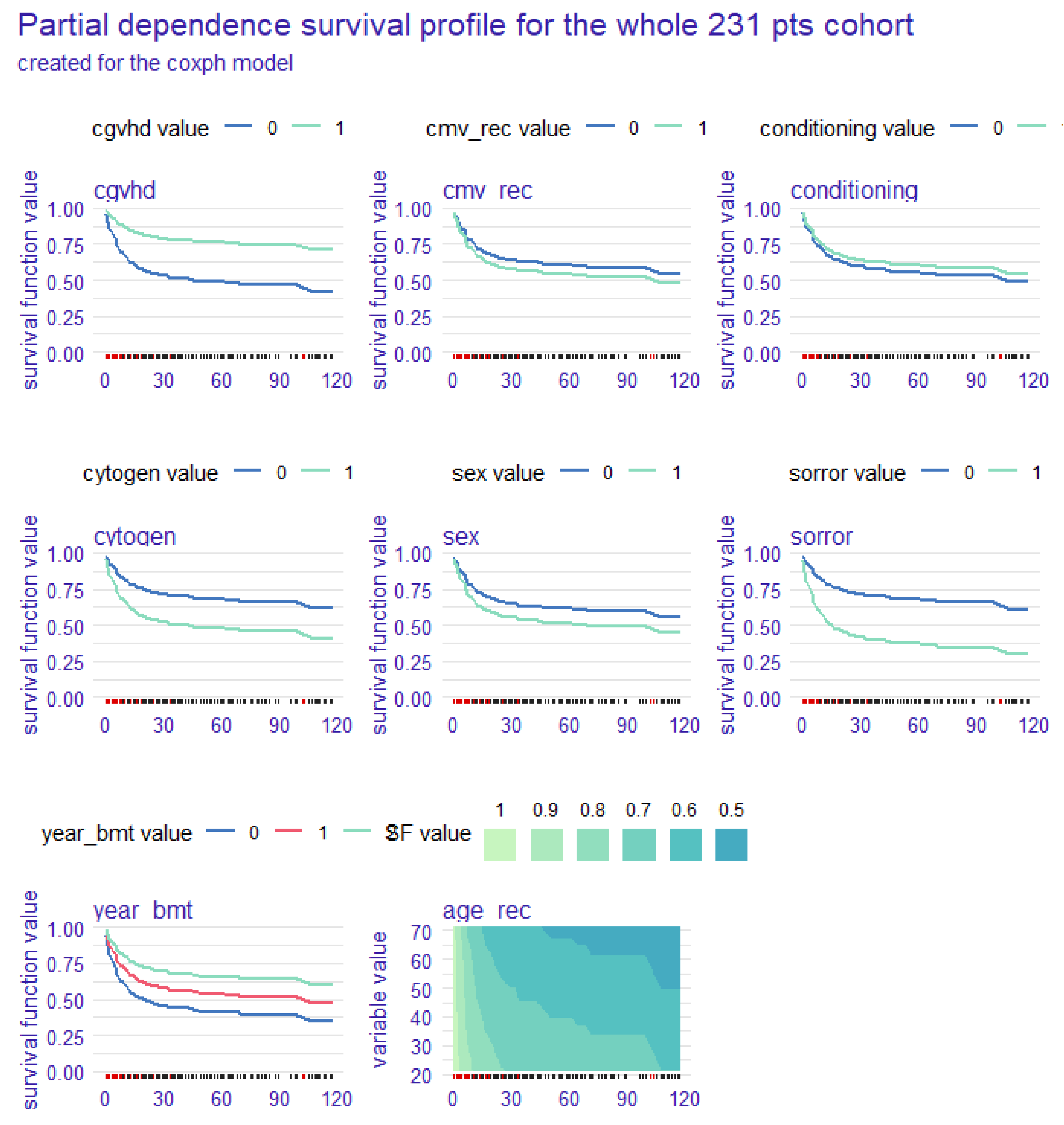
2b—Global explanation: partial dependence survival profile (PDP) for the whole cohort

3a—Local explanation: SurvSHAP(t) plot per single patient

3b—Local explanation: SurvLIME plot per single patient

3c—Local explanation: ceteris paribus survival profile per single patient

3.1. Model Performance for the Whole Cohort

A set of performance measures on model quality was estimated using the Brier score (the lower, the better), the C/D AUC (the higher, the better) and the C-index (the higher, the better); all these metrics were reported on the y-axis. Random survival forest generally overperformed coxph in each metric (Figure 1, XAI as bar plots) and during the whole follow-up (Figure 2, XAI as time-dependent estimations): the longest observation occurred at 163 mos after BMT. Brier score was 0.180 vs. 0.193, C/D AUC was 0.668 vs. 0.623, while C-index was 0.775 vs. 0.743 for rfsrc vs. coxph, respectively. The better prediction power of rfsrc had a limitation in its more difficult interpretability, compared to coxph;

Table 2. Univariate and multivariate Cox proportional hazard models for Overall Survival after allogeneic HSCT.

Univariate Models			Multivariate Model
	HR (95% CI)	p	HR (95%CI)	p
Age		0.080		0.262
(40–60 vs. <40 years)	1.30 (0.73–2.31)	0.369	0.56 (0.23–1.38)	0.210
(>60 vs. <40 years)	1.93 (1.04–3.59)	0.038	0.91 (0.37–2.25)	0.839
Gender (male vs. female)	1.30 (0.87–1.95)	0.201	2.25 (1.18–4.29)	0.014
HCT-CI (≥3 vs. 0–2)	3.11 (1.86–5.21)	<0.001	3.10 (1.70–5.65)	<0.001
Cytogenetics (interm/high vs. low risk)	1.80 (1.02–3.20)	0.044	1.54 (0.81–2.92)	0.191
CMV recipient status (positive vs. negative)	1.69 (1.04–2.76)	0.035	1.04 (0.47–2.32)	0.925
Conditioning (RIC vs. MAC)	1.71 (1.02–2.90)	0.044	1.04 (0.44–2.47)	0.933
Year of transplant		0.007		0.382
(2013–2017 vs. 2008–2012)	0.51 (0.32–0.82)	0.005	1.64 (0.38–6.99)	0.506
(2018–2021 vs. 2008–2012)	0.49 (0.29–0.82)	0.007	1.04 (0.24–4.56)	0.959
Chronic GvHD moderate-severe (yes vs. no) *	0.19 (0.09–0.40)	<0.001	0.22 (0.09–0.53)	<0.001

* Treated as time-dependent variable. Abbreviations: HR hazard ratio, CI confidence interval, HCT-CI hematopoietic cell transplantation-comorbidity index, CMV cytomegalovirus, RIC reduced intensity conditioning, MAC myeloablative conditioning, GvHD graft versus host disease.

reports the classical uni- and multi-variate Cox proportional hazards model results for OS, as a complement to the graphical XAI.

3.2. Global Explanation: Time-Dependent Feature Importance for the Whole Cohort

Time-dependent variable importance for the whole cohort has been investigated using two different approaches, the Brier score loss after permutation (Figure 3) and the C/D AUC loss after permutation (Figure 4), both for coxph and rfsrc. The y-axis now represents the change in the loss function after permuting each covariate: variable importance does change over time and the highest increases in the loss function were associated with the most significant determinants for OS. Coxph and rfsrc showed quite similar results: HCT-CI (labelled as sorror) was the worst independent risk factor for OS, having a more marked time-dependent effect by the Brier score loss. On the other hand, either a chronic GVHD occurrence (due to its well-known graft-versus-leukemia effect) or a more recent year of transplantation played a protective role on OS, influencing model predictions especially for long-survivor patients.

3.3. Global Explanation: Partial Dependence Survival Profile for the Whole Cohort

Figure 5 and Figure 6 report the partial dependence survival profiles (PDP) for coxph and rfsrc models, respectively. Survival function values for any covariate are on the y-axis; the wider their difference between/among the levels of a factor, the larger the impact that the same factor played on OS. PDPs show how OS would change for the whole cohort, changing the value of a single determinant but keeping unchanged all the other ones. As for categorical determinants, cGVHD occurrence (coded 1 on the plot), HCT-CI ≥3 (high comorbidities, coded 1) and early years of BMT were the most significant unfavorable predictors, both in coxph and rfsrc; the other categorical risk factors had no role on OS. Of note, while coxph identified three time periods with different survival, rfsrc picked up two, clustering together the two oldest time frames (2018–2021 vs. 2008–2017). As for continuous covariates, the progressive drop in survival function for recipient age is better modeled by coxph: age appears to be stratified in 5 classes, associated with a different survival, the youngest one to the longest OS. Interestingly, moving to a different modeling strategy and using the maximally selected rank statistics to estimate potential optimal cutpoints for continuous covariates, an age equal to 36 years would allow us to stratify OS in two asymmetrical subgroups (up to 36 years, 26 patients; over 36 years, 205 patients).

3.4. Local Explanation: SurvSHAP(t) Plot per Single Patient

Moving from the predictions for the whole cohort to those for a single statistical unit (single observation), XAI for survival has been used to explain the modeling results for a randomly selected patient (pt#10): woman, aged 62 years at BMT, low-risk cytogenetic profile, positive CMV status, HCT-CI 0–2 (low/intermediate comorbidities), who received a myeloablative conditioning regimen BMT in 2011, who was not affected by chronic GVHD and who died in 2019, 102 months after BMT. SurvSHAP(t) plots allow the study that the time-dependent survival contribute exerted on OS by each risk factor for a selected case: positive SurvSHAP(t) values, plotted for each covariate on the y-axis, were associated with a shorter OS, while negative ones with a longer OS. Thus, the time-dependent estimation of SurvSHAP(t) values referred to this patient were reported in Figure 7. Unlike the whole cohort, age and sex emerged as unfavorable prognostic factors, both for coxph and rfsrc. Overall survival takes into account death for any cause, and this female patient died for breast cancer (second cancer?): indeed, SurvSHAP(t) identified as main OS determinants age and female gender, rather than the other classical hematological and transplant-related risk factors.

3.5. Local Explanation: SurvLIME Plot per Single Patient

The SurvLIME plot approach is quite similar to the previous one, detecting the most influential survival predictors for a single, selected patient: always pt#10, in our case. Making survival predictions for this patient and attributing variable importance for OS, the SurvLIME plot is divided into two parts (Figure 8 and Figure 9, for coxph and rfsrc models, respectively). The left one shows that increasing age and positive recipient CMV status were the most unfavorable OS predictors for this woman, both by coxph and rfsrc: the higher the SurvLIME local importance value, the lower the survival chances. The right one compares either the coxph or rfsrc model predictions to those deriving from a surrogate proportional hazard model at the local area: the closer they are, the more accurate the survival estimation. Of note, since the median follow-up for the whole cohort was 56 months, OS estimations became less accurate over the course of time, both for coxph and rfsrc.

3.6. Local Explanation: Ceteris Paribus Survival Profile per Single Patient

Figure 10 and Figure 11 report the ceteris paribus survival profiles (CPP), always referring to patient #10, for coxph and rfsrc, respectively: these graphics are equivalent to the PDP ones, but related to a single observation. As with PDPs, even with CPPs survival function, lower values (on y-axis) were associated with a poorer OS, and the most significant determinants were those with the largest difference between/among the levels of the categorical variables. Patient values for continuous covariates (pt#10 was 62 years old) are highlighted as a red line. CPPs show how survival function would change for pt#10, changing the value of one covariate and keeping unchanged all the other ones; in our case, most determinants affected OS, except for cytogenetic risk, CMV status and conditioning regimen. Of note, the eventual occurrence of a chronic GVHD would appear as a critical favorable OS determinant by coxph (as clinically expected), while not by rfsrc.

4. Discussion

The decision-making process in oncohematology does very often rely on survival data, and it could benefit from the results of different ML models. At the same time, exploring and explaining predictive survival models with censored observations is a hard task: hence the added value of XAI for survival algorithms. The survex package for R is a very interesting tool, coming from the Biecek group in Warsaw: it offers a large and complete choice of ML model explainers. All analyses can be conducted under a common, uniform interface; in our case, it allows to easily explore and compare results coming from two different survival models for a bone marrow transplantation trial, the proportional hazard regression model and the random survival forest.

A correct workflow with survex has to start examining the model quality by measuring its performance, both for coxph and rsfrc. Three different metric values are available (C-index, integrated C/D AUC and integrated Brier score); of note, the x-axis reports the scores’ variation over follow-up course. The metric performances are almost comparable; the slight overperformance of rsfrc has a cost, namely its less immediate interpretation. As usual, model performance is influenced by the global sample size: our trial had a median dimension, in the field of BMT clinical research.

As a second step, a series of global explanations is dedicated to exploring model predictions for the whole patient cohort. The estimation of permutational variable importance is a time-dependent process, which can be reported along a time course, using two different loss functions (Brier score and 1—CD/AUC): the highest increase in the loss function, the most importance for the covariate. Moreover, partial dependence survival profiles can be plotted for any covariate, either categorical or continuous: this analysis shows the risk factors contribute to the global model, changing the value of one determinant at a time.

Finally, another series of local explanations allows to explore a model’s prediction for a single, selected observation. Thus, it is possible to estimate how any determinant impacted on the OS for each patient, sometimes revealing dramatic, unexpected differences among them: a notable improvement compared to classical survival models. Three local explanations are available, with different visualizations. The SurvSHAP(t) function for any risk factor decreases, when OS decreases; the SurvLIME function shows the most important OS determinants and their favorable/unfavorable effect on time course. The ceteris paribus survival profile, by analogy to the partial dependence survival plots for the whole cohort, allows to graphically estimate the role on OS of each risk factor for any single observation.

A critical point in our research does depend on the lack of separate training/validation/test datasets. This has been a forced choice, due to the population sample size, which did not allow an effective dataset splitting. Indeed, more than on OS results’ confirmation, this research focused on the feasibility of XAI for survival in oncohematology using the R survex environment.

In conclusion, the survex package for R opens the door to a complete, direct and intuitive interpretation of survival models, either for the entire population or for selected patients. It allows one to compare results coming from different survival modeling approaches, like, e.g., the proportional hazards regression model and random survival forest, using XAI for survival to explain their results.

References

1. Joshi, G.; Jain, A.; Adhikari, S.; Garg, H.; Bhandari, M. FDA approved Artificial Intelligence and Machine Learning (AI/ML)-Enabled Medical Devices: An. updated 2022 landscape. MedRxiv Prepr. Serv. Health Sci. 2022. [Google Scholar] [CrossRef]
2. Salah, H.T.; Muhsen, I.N.; Salama, M.E.; Owaidah, T.; Hashmi, S.K. Machine learning applications in the diagnosis of leukemia: Current trends and future directions. Int. J. Lab. Hematol. 2019, 41, 717–725. [Google Scholar] [CrossRef] [PubMed]
3. Shouval, R.; Fein, J.A.; Savani, B.; Mohty, M.; Nagler, A. Machine learning and artificial intelligence in haematology. Br. J. Haematol. 2021, 192, 239–250. [Google Scholar] [CrossRef] [PubMed]
4. Muhsen, I.N.; Hashmi, S.K. Utilizing machine learning in predictive modeling: What’s next? Bone Marrow Transpl. 2022, 57, 699–700. [Google Scholar] [CrossRef] [PubMed]
5. Barredo Arrieta, A.; Díaz-Rodríguez, N.; Del Ser, J.; Bennetot, A.; Tabik, S.; Barbado, A.; Garcia, S.; Gil-Lopez, S.; Molina, D.; Benjamins, R.; et al. Explainable Artificial Intelligence (XAI): Concepts, taxonomies, opportunities and challenges toward responsible AI. Inf. Fusion. 2020, 58, 82–115. [Google Scholar]
6. Knapic, S.; Malhi, A.; Saluja, R.; Främling, K. Explainable Artificial Intelligence for Human Decision Support System in the Medical Domain. Mach. Learn. Knowl. Extr. 2021, 3, 740–770. [Google Scholar] [CrossRef]
7. Di Martino, F.; Delmastro, F. Explainable AI for clinical and remote health applications: A survey on tabular and time series data. Artif. Intell. Rev. 2023, 56, 5261–5315. [Google Scholar] [PubMed]
8. Biecek, P.; Burzykowski, T. Explanatory Model Analysis; Chapman and Hall/CRC: New York, NY, USA, 2021. [Google Scholar]
9. Baniecki, H.; Parzych, D.; Biecek, P. The grammar of interactive explanatory model analysis. Data Min. Knowl. Disc. 2023, 14, 1–37. [Google Scholar]
10. Spytek, M.; Krzyziński, M.; Baniecki, H.; Biecek, P. Survex: Explainable Machine Learning in Survival Analysis; R Package Version 1.0.0.9000. Available online: https://modeloriented.github.io/survex/ (accessed on 15 August 2023).
11. Kovalev, M.S.; Utkin, L.V.; Kasimov, E.M. SurvLIME: A method for explaining machine learning survival models. Knowl.-Based Syst. 2020, 203, 106164. [Google Scholar]
12. Krzyziński, M.; Spytek, M.; Baniecki, H.; Biecek, P. SurvSHAP(t): Time-dependent explanations of machine learning survival models. Knowl.-Based Syst. 2023, 262, 110234. [Google Scholar]
13. Cox, D.R. Regression models and life-tables. J. Royal. Stat. Soc. Ser. B 1972, 34, 187–220. [Google Scholar] [CrossRef]
14. Ishwaran, H.; Kogalur, U.B.; Blackstone, E.H.; Lauer, M.S. Random survival forests. Ann. Appl. Stat. 2008, 2, 841–860. [Google Scholar]
15. Lo Schirico, M.; Passera, R.; Gill, J.; Dellacasa, C.; Dogliotti, I.; Giaccone, L.; Zompi, S.; Busca, A. Graft-versus-host disease prophylaxis with anti-thymocyte globulin in patients receiving stem cell transplantation from unrelated donors: An observational retrospective single-center study. Cancers 2023, 15, 2761. [Google Scholar]
Figure 1. Model performance for the whole cohort, 1, XAI as bar plots.
Biomedinformatics 03 00048 g001
Figure 2. Model performance for the whole cohort, XAI as time-dependent estimations.
Biomedinformatics 03 00048 g002
Figure 3. Global explanation: time-dependent feature importance for the whole cohort, Brier score loss after permutation.
Biomedinformatics 03 00048 g003
Figure 4. Global explanation: time-dependent feature importance for the whole cohort, C/D AUC loss after permutation.
Biomedinformatics 03 00048 g004
Figure 5. Global explanation: partial dependence survival profile for the whole cohort, coxph model.
Biomedinformatics 03 00048 g005
Figure 6. Global explanation: partial dependence survival profile for the whole cohort, rfsrc model.
Biomedinformatics 03 00048 g006
Figure 7. Local explanation: SurvSHAP(t) plot for a single patient.
Biomedinformatics 03 00048 g007
Figure 8. Local explanation: SurvLIME plot for a single patient, coxph model.
Biomedinformatics 03 00048 g008
Figure 9. Local explanation: SurvLIME plot for a single patient, rfsrc model.
Biomedinformatics 03 00048 g009
Figure 10. Local explanation: ceteris paribus survival profile for a single patient, coxph model.
Biomedinformatics 03 00048 g010
Figure 11. Local explanation: ceteris paribus survival profile for a single patient, rfsrc model.
Biomedinformatics 03 00048 g011