A Stochastic Multivariate Irregularly Sampled Time Series Imputation Method for Electronic Health Records

Abstract

Electronic health records (EHRs) can be very difficult to analyze since they usually contain many missing values. To build an efficient predictive model, a complete dataset is necessary. An EHR usually contains high-dimensional longitudinal time series data. Most commonly used imputation methods do not consider the importance of temporal information embedded in EHR data. Besides, most time-dependent neural networks such as recurrent neural networks (RNNs) inherently consider the time steps to be equal, which in many cases, is not appropriate. This study presents a method using the gated recurrent unit (GRU), neural ordinary differential equations (ODEs), and Bayesian estimation to incorporate the temporal information and impute sporadically observed time series measurements in high-dimensional EHR data.

1. Introduction and Background

One of the biggest challenges to work with electronic health record (EHR) data is that there are many missing values. This issue incorporates uncertainty in the predictive model if the missing instances are imputed. Common imputation methods usually do not consider the temporal information, which is crucial for time series analysis. Moreover, most time series analysis methods ignore the time gap between measurements or assume that the time gaps are equal. In this study, we investigated time series imputation with irregular time gaps and propose a method based on neural ordinary differential equations (ODEs), recurrent neural networks (RNNs), and Bayesian estimation. This method offers a robust imputation of sporadically sampled multivariate time series measurements obtained from different patients.

Many data imputation techniques have been developed over the years. In real-life problems, it is very common to have multiple missing attributes for a particular dataset. In the literature, most datasets have 30% to 50% missing values, and they have been imputed using various techniques [1]. There are mostly two techniques widely used for data imputation. These are statistical techniques and machine-learning-based techniques. Among the statistical techniques, expectation minimization (EM), the Gaussian mixture model (GMM), Markov chain Monte Carlo (MCMC), naive Bayes (NB), principal component analysis (PCA), etc., have been used frequently [1]. Among the machine-learning-based techniques, the Gaussian process for machine learning (GPML) (see [2]), support vector machines (SVMs) [3,4], k-nearest neighbors (k-NNs) [5], decision trees (DTs) [6], and artificial neural networks (ANNs) [7] have been heavily used in the literature.

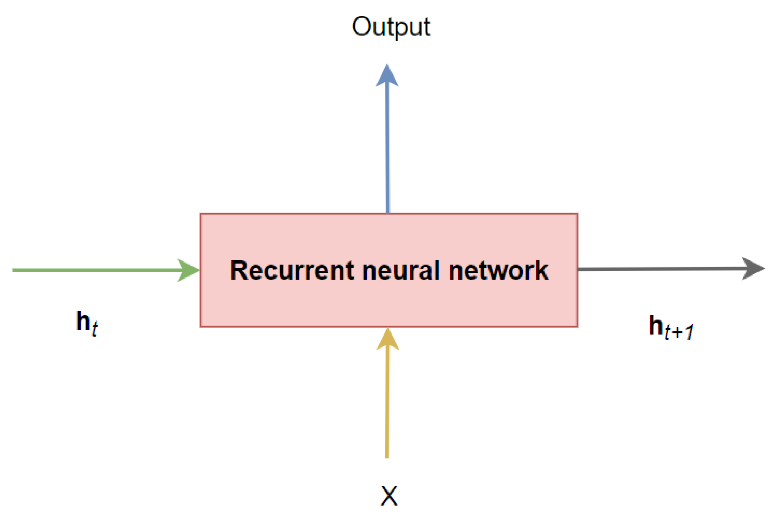
In recent years, longitudinal data imputation has been necessary specially in EHRs. However, many imputation methods only consider the data without the very important element–temporal information. However, there are many time series imputation methods that only consider equal time steps. Our research focuses on a time series imputation method that can deal with sporadically observed time series measurements obtained from EHRs. The major key components to implement this imputation method are neural ODEs [8], which parameterize the derivative of a neural network’s hidden state. As compared to the popular residual neural networks, neural ODEs have superior memory and parameter efficiency. Neural ODEs can easily deal with continuous time series, unlike recurrent neural networks, which require discretization. In a follow-up study, latent ODEs were proposed for irregularly sampled (e.g., sporadic) time series [9]. This method (called ODE-RNN) is presented as an alternative to autoregressive models. However, neural ODEs [8] use RNNs as the recognition network to estimate the posterior probabilities. However, that approach is more appropriate for continuous time series modeling with regularly sampled data. Therefore, the ODE-RNN [9] has been introduced as the recognition network to deal with irregularly sampled continuous time series analysis. 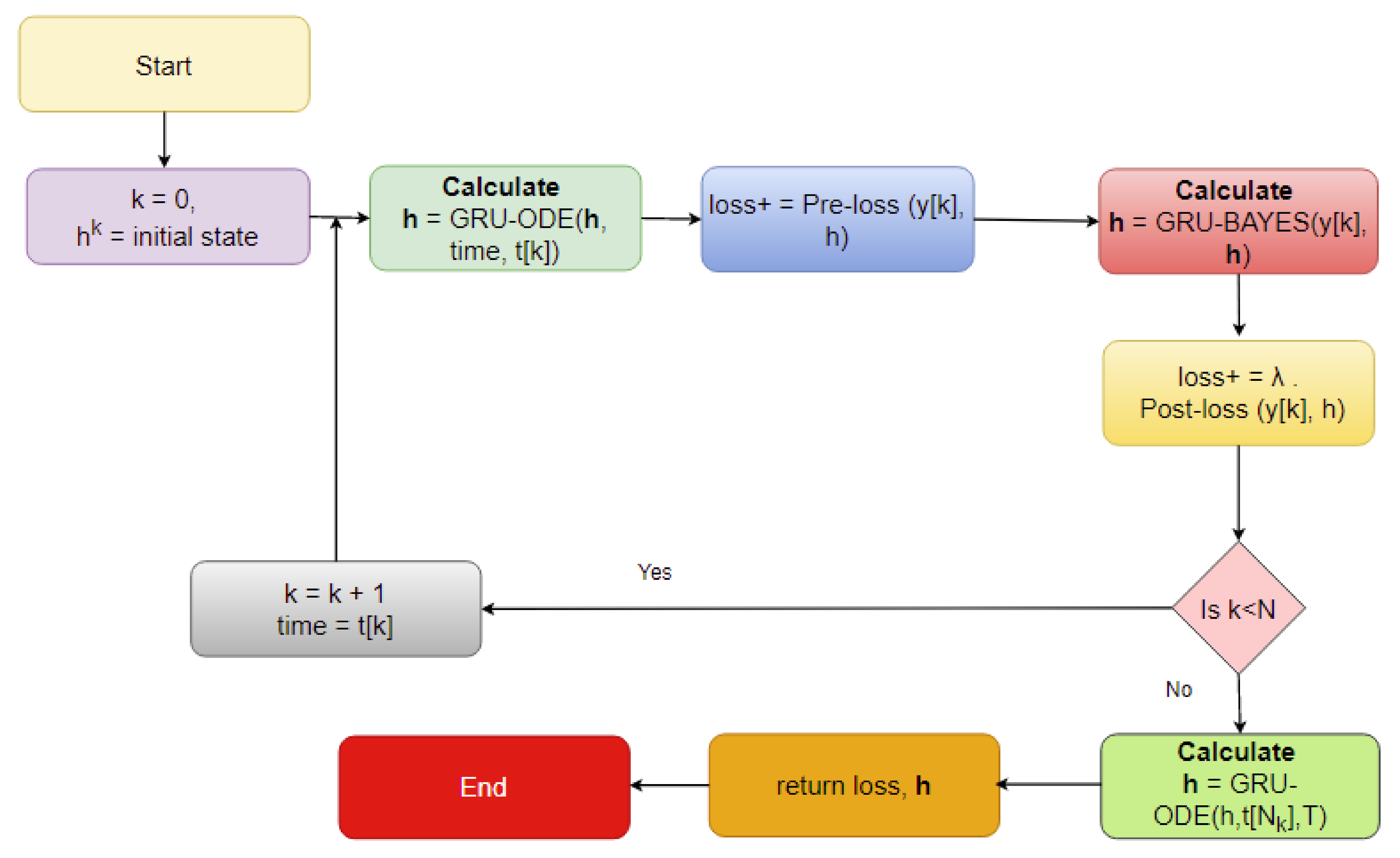Combined with neural ODEs and the GRU, a Bayesian update [10] is proposed that uses a predictive (with observation masking) method (called the GRU-ODE-Bayes method) to include only the available observations to update the predicted values along the multivariate time series. However, this method does not impute the missing values; rather, it performs zero- or mean-value padding. The GRU-ODE-Bayes method assumes that the observations are sampled from a multidimensional stochastic process whose dynamics can be explained by a Weiner process. The examples include the stochastic Brusselator process [11], the double-Ornstein–Uhlenbeck (OU) stochastic differential equations [12], etc. The authors showed that their method achieved better results than the GRU-D [13,14], minimal gated unit or minimal GRU [15], and other popular methods. In another recent study [16], a bidirectional recurrent imputation for time series (BRITS) was proposed. This algorithm uses both a forward and backward feeding of inputs to the RNN and simultaneously imputes the missing values. However, the BRITS does not allow the stochastic imputation of time series data. The BRITS is composed of a recurrent component and a regression component for imputation. The authors also presented a unidirectional approach called the RITS and claimed that the process was slower compared to the BRITS. Among other RNN-based models, the multidirectional RNN (M-RNN) provides good imputation results [17]. This study aims to develop a robust multivariate stochastic imputation technique for irregular time series that will fill this research gap.

2. Data Processing

To develop a good predictive model, a reliable database is very crucial. The data need to be authentic and mostly accurate. Any big-data-driven research highly depends on the quality of the data being used. In this study, a very popular dataset [13,18,19,20] named the Medical Information Mart for Intensive Care (MIMIC) clinical database was explored and analyzed. This dataset contains intensive care unit (ICU) admission records of patients admitted to Beth Israel Deaconess Medical Center in Boston, Massachusetts, from 2001 to 2012. This database has several versions. In this study, MIMIC III Version 1.4 was used, which is the latest. It contains de-identified electronic medical records, demographic information, and billing information for ICU-admitted patients. Many of these records contain timestamps of clinical events, nurse-verified physiological measurements, routine vital signs, check-up information, etc. However, this database is only available after completing a required course and acknowledging a data use agreement.

After accessing the electronic records from the MIMIC III clinical database, a clean dataset needs to be formed that can be useful for analysis. As most other databases, MIMIC III provides its users with different types of structured and unstructured data records that must be cleaned prior to performing any data-driven analysis. Furthermore, the electronic records sometimes have different artifacts associated with them. Data cleaning tends to be more difficult in the case of large databases such as MIMIC III. The search algorithms for the desired attributes need to designed in a way that they can extract the necessary information efficiently. There are hardware and software limitations due to which it becomes very difficult to carry out large matrix operations in traditional computers. Since the analysis highly depends on the data quality, a proper cleaning process should be selected and performed carefully. There might be anomalies in the chosen dataset that should be properly dealt with before any analysis.

2.1. Data Description

The MIMIC-III database is an information storehouse for critical care patients. Therefore, it needs to deal with proper care and privacy. To access the data, one needs to request access formally through the Physionet website (https://www.physionet.org) (last accessed on 15 November 2021). Two important steps need to be followed to access the data. The first one is to take a recognized course and comply with the Health Insurance Portability and Accountability Act (HIPAA) requirements. The second step is to sign a data use agreement that includes the appropriate data usage policy, security standards, and preventing identification efforts. Once the request is submitted, the approval comes within a week. Then, the data can be accessed from the server or can be stored in local storage. More information can be obtained by visiting the official MIMIC website (https://physionet.org/content/mimiciii/1.4/) (last accessed on 15 November 2021).

There are 26 tables in total in the MIMIC-III database (see Appendix A,

Table A1. All tables of MIMIC III and their total records.

Patient Tracking		ICU Data
Table name	Total records	Table name	Total records
Admissions	58,976	Chartevents	330,712,483
ICUstays	61,532	Inputevents_cv	17,527,935
Patients	46,520	Inputevents_mv	3,618,991
Callout	34,499	Datetimeevents	4,485,937
Transfers	261,897	Outputevents	4,349,218
-	-	Procedureevents_mv	258,066
Hospital Data		Dimension Tables
Table name	Total records	Table name	Total records
Caregivers	7567	D_CPT	134
CPTevents	573,146	D_ICD_Procedures	3882
Diagnoses_icd	651,047	D_Items	12,487
DRGcodes	125,557	D_ICD_Diagnoses	14,567
Labevents	27,854,055	D_labitems	753
Microbiologyevents	631,726
Noteevents	2,083,180
Prescriptions	4,156,450
Procedures_icd	240,095
Services	73,343

). In this subsection, we mainly discuss the tables that were directly used for the analysis. Since our goal was to extract as many CHF-related variables as possible, we needed to explore different tables and match records with mostly unique patient IDs and sometimes with admission IDs. Different tables are linked together to compile the dataset that we needed. The tables are described in the following paragraphs.

The “Admissions” table provides unique hospital admission information for each patient. It reports the admission ID, ICUstay ID, date of admission, admission type, discharge location, diagnosis, insurance, language, religion, marital status, age, ethnicity, etc. This can be linked with other tables via the admission ID and patient ID.

The “Patients” table provides demographic information for 46,520 unique patients. It contains the patient ID, admission ID, date of birth, date of death, gender, hospital expire flag, etc.

The “Chartevents” table is the largest table in the entire MIMIC III database. This has about 330,712,483 records. This table provides the patient ID, admission ID, item ID, and the corresponding routine physiological measurements of each patient from time to time.

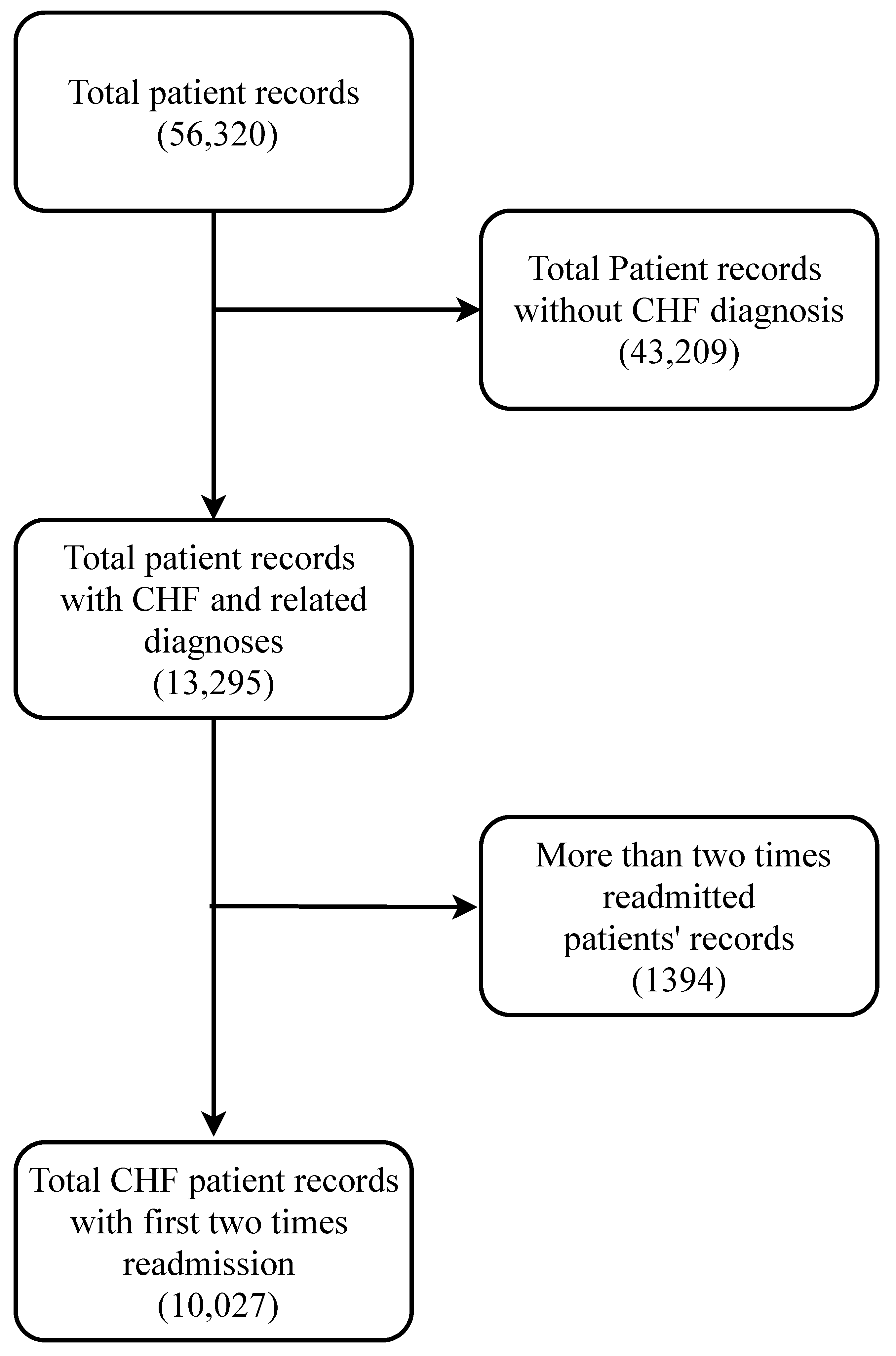
The “D_ICD_diagnosis” table contains unique patient IDs, unique hospital admission IDs, and International Coding Definitions Version 9 (ICD-9) for each of the 14,567 diagnosis categories. The code for CHF diagnosis is 4280.

The “D_items” table has 12,487 records of items used to treat different patients. Routine vital signs such as blood pressure, heart rate, white blood cell count (WBC), respiratory rate, and other numerical variables are listed here with distinct item IDs.

2.2. Data Cleaning

Before any type of analysis, the subset of the entire database, that is of interest, needs to be extracted. Data cleaning can be a very tedious process, especially in the case of such huge clinical databases as MIMIC III. Figure 1 shows the data-cleaning steps. The data-cleaning steps are quite challenging at times. At first, all patient records (56,320) were assessed. These records mostly contain the demographic information such as age, gender, religion, etc. There is some hospital-related information available as well, such as admission type, discharge location, length of stay, etc. Since this study focuses on CHF (and some related diagnoses)-diagnosed patients only, those were extracted using the ICD-9 diagnosis codes. This totaled 13,295 patients. Among these patients, many of them had been readmitted multiple times with the maximum number of readmissions as high as 13. If a patient is never readmitted or followed up, we kept their admission record as is. In the case of multiple readmitted patients, we only considered their first time readmission record and discarded the subsequent ones. Then, all the numerical and categorical features were joined to the patient list (total 10,027 patients) according to their unique ICU stay IDs.

2.3. Patient Cohort Selection

As mentioned earlier, mostly CHF patients were considered for this study. Along with CHF, the following diagnoses were also considered, as shown in

Table 1. All the diagnoses considered for patient cohort selection.

ICD-9 Code	Diagnosis Description
4280	Congestive heart failure, unspecified
4281	Left heart failure
4289	Heart failure, unspecified
42820	Systolic heart failure, unspecified
42821	Acute systolic heart failure
42822	Chronic systolic heart failure
42823	Acute or chronic systolic heart failure
42830	Diastolic heart failure, unspecified
42831	Acute diastolic heart failure
42832	Chronic diastolic heart failure
42833	Acute or chronic diastolic heart failure
42840	Combined systolic and diastolic heart failure, unspecified
42841	Acute combined systolic and diastolic heart failure
42842	Chronic combined systolic and diastolic heart failure
42843	Acute or chronic combined systolic and diastolic heart failure

.

2.4. Numerical Variables

EHRs contain time series measurements of different patients. It is sometimes very difficult to understand the contributing features of a certain outcome.

Table 2. All numeric variables and their missing ratios.

Name	%Miss	Name	%Miss
WBC	0.721	Cardiac Index	0.790
ALT	0.765	Central Venous Pressure	0.876
Arterial Base Excess	0.699	Chloride	0.720
Arterial CO2(Calc)	0.693	Heart Rate	0.555
Arterial PaCO2	0.696	Direct Bilirubin	0.954
Arterial PaO2	0.695	FiO2 Set	0.664
Arterial pH	0.683	GCS Total	0.513
BUN	0.509	Glucose	0.721
Creatinine	0.720	INR	0.512
Calcium	0.731	Potassium	0.720
Magnesium	0.724	Mean Airway Pressure	0.903
Sodium	0.720	RBC	0.591
PAO2	0.988	Respiratory Rate	0.541
PEEP Set	0.902	SaO2	0.770
Plateau Pressure	0.914	Arterial Blood Pressure Diastolic	0.845
Platelets	0.590	Temperature F	0.462
Prothrombin time	0.541	Total Bilirubin	0.712
PTT	0.543	Total Protein	0.980

shows the chosen predictor numerical variables [21] for this analysis. The variables were selected based on multiple studies [22,23,24] and their importance to CHF readmission prediction.

2.5. Time Series Extraction

This section presents the filtering criteria and the personalized time series extraction process from the MIMIC-III v1.4 database. As mentioned in earlier sections, there were about 10,000 unique patients having CHF and other related diagnoses. For each of these patients, a unique time series was extracted that contained different types of measurements obtained for different items (e.g., heart rate, glucose, BUN, etc.). Figure 2 shows a sample patient with different item measurements taken at irregular intervals along the horizontal axis. Although it shows measurements beyond 48 h from discharge, this study only considered measurements up to 48 h from discharge. It is important to note that all the item measurements might not be available for all patients. Therefore, the time series imputation became more challenging due to the lack of data.

First, the patients were sorted using their unique ICU stay IDs. This ID distinguishes every single ICU stay of a patient. There were some patients who had been readmitted to the ICU more than once during the same hospital admission. In these cases, they usually had a the same admission ID, but different ICU stay IDs. That is why we chose to identify patients by their ICU stay IDs. However, their subject IDs and admission IDs are also stored in the patient database. A search algorithm was deployed to find each patient’s measurement during his/her unique ICU stay.

3. Methodology

This section describes and implements the multivariate irregularly sampled time series imputation method that was based on neural ODEs, GRU, LSTM, and Bayesian estimation. It is important to discuss the useful technical details of this method so that it can be explained easily. The flowchart and mathematical notations are used for the explanation as necessary. are applicable here, as well. In the following sections, the imputation problem is introduced, and the methods for overcoming this challenge are discussed.

Any EHR database contains numerous vital measurement information for ICU patients. Due to many physiological factors, these measurements are not taken at the same time intervals. For predictive modeling and other data scientific procedures, regular intervals are usually expected. Therefore, EHR data can be challenging due to these irregular measurements.

The problem is to develop an imputation method that can perform two challenging tasks: capture the temporal information from irregularly sampled time series measurements and impute time series with high missing ratios. However, the standard imputation methods hardly consider temporal information and are mostly suitable for regular time series. This section describes the technical and mathematical details for the multivariate imputation method. The important components of the method—neural the ODE, GRU and Bayesian estimation—are discussed sequentially. To summarize the steps, the algorithm is presented in a compact version that is easier to understand. From this point, the proposed method is called the GRU LSTM ODE BAYES Imputation (GOBI) method.

3.1. Recurrent Neural Networks

Recurrent neural networks are a special type of artificial neural network that are able to exhibit temporal dynamic behavior in sequence data. They can process temporal information from the current state to the next state using hidden layers. However, the conventional RNN suffers from the vanishing gradient problem. This means that the weights of the neural network are more difficult to train further down the sequence because the loss function tends to be very close to zero. To avoid this problem, mostly two types of gated RNNs are used—long short-term memory (LSTM) and the gated recurrent unit (GRU). These two special types of RNNs were used in this study. Defining X as the input and $h_t$ and $h_{t+1}$ as the previous and current hidden layers, the simple structure of an RNN layer is shown in Figure 3.

3.2. Neural ODEs

Neural ODEs [8] are useful for continuous-depth neural networks. This method involves performing a reverse-mode differentiation technique (e.g., backpropagation), which is quite difficult to train. While solving the ODEs, the adjoint sensitivity method is used. This approach usually takes less time and calculation effort. A scalar-valued loss function L [8] as described in Equation (1) is minimized, whose input comes from the ODE solver.

$$L\left(\mathbf{h}\left(t_1\right)\right)=L\left(\mathbf{h}\left(t_0\right)+{\int }_{t_0}^{t_1}f\left(\mathbf{h}\left(t\right),t,\theta \right)dt\right)$$

(1)

Here,

• $h\left(t_1\right)$ = current hidden state;
• $h\left(t_0\right)$ = initial hidden state;
• $t_0$ = initial time;
• $t_1$ = current time;
• $\theta$ = weight of neurons at synapses;
• f = hidden unit dynamics function.

The loss function L incorporates all the time points (e.g., states) in the time series. The adjoint states help to calculate the gradients with respect to $\theta$, as needed along the time sequence. Defining the adjoint $a\left(t\right)=\frac{\delta L}{\delta t}$ and taking the derivative yield [8],

$$\frac{d\mathbf{a}\left(t\right)}{dt}=-\mathbf{a}{\left(t\right)}^T\frac{df\left(\mathbf{h}\left(t\right),t,\theta \right)}{d\mathbf{h}}$$

(2)

Note that Equation (2) allows the computation of gradients along the time sequence. However, the gradient of L with respect to $\theta$ is calculated by propagating backwards. This yields (See [8])),

$$\frac{dL}{d\theta }={\int }_{t_1}^{t_0}\mathbf{a}{\left(t\right)}^T\frac{df\left(\mathbf{h}\left(t\right),t,\theta \right)}{d\theta }dt$$

(3)

Therefore, the above two equations can be efficiently calculated by any regular auto-differentiation packages.

If the observations $y_i$ are sampled from the realizations of a D-dimensional stochastic process $\mathbf{Y}\left(t\right)$, the internal dynamics can be expressed as an unknown stochastic differential equation (SDE) as the following:

$$d\mathbf{Y}\left(t\right)=\mu \left(\mathbf{Y}\left(t\right)\right)dt+\sigma \left(\mathbf{Y}\left(t\right)\right)d\mathbf{W}\left(t\right)$$

(4)

Here,

• $dW\left(t\right)$ = Weiner process;
• $\mu$ = mean of the probability density function of $\mathbf{Y}\left(t\right)$;
• $\sigma$ = covariance of probability density function of $\mathbf{Y}\left(t\right)$.

Then, the distribution of $\mathbf{Y}\left(t\right)$ evolves according to the Fokker–Planck equation [10].

3.3. GRU and the Differential Form of Its Hidden State

The GRU is a type of RNN that requires less time and calculation effort than its counterpart LSTM. However, there is no clear indication of the superiority of their performance on real-world datasets. As reported by many authors [13,15,17], the GRU and LSTM usually perform head to head with a slight edge over each other on different datasets and in different configurations. Figure 4 shows a standard GRU cell configuration. There are two main gates in a GRU: reset gate and update gate. This configuration makes the GRU very simple to train and take less time to compute all the parameters.

As seen in Figure 4, a standard GRU cell contains the following elements [10]:

$$\begin{array}{ccc}\hfill {\mathbf{r}}_t& =& \sigma \left(W_r{\mathbf{x}}_t+U_r{\mathbf{h}}_{t-1}+{\mathbf{b}}_r\right)\hfill \end{array}$$

(5)

$$\begin{array}{ccc}\hfill {\mathbf{z}}_t& =& \sigma \left(W_z{\mathbf{x}}_t+U_z{\mathbf{h}}_{t-1}+{\mathbf{b}}_z\right)\hfill \end{array}$$

(6)

$$\begin{array}{ccc}\hfill {\mathbf{g}}_t& =& tanh\left(W_h{\mathbf{x}}_t+U_h\left({\mathbf{r}}_t\odot {\mathbf{h}}_{t-1}\right)+{\mathbf{b}}_h\right)\hfill \end{array}$$

(7)

Here, ${\mathbf{r}}_t$, ${\mathbf{z}}_t$, and ${\mathbf{g}}_t$ denote the reset, update, and forget gate, respectively. Furthermore, ⊙ corresponds to the elementwise product. Two matrices $W\in {\mathrm{I}\mathrm{R}}^{H\times D}$ and $b\in {\mathrm{I}\mathrm{R}}^{H\times H}$ denoting the weight and bias vectors are the cell parameters. H and D are the dimensions of the hidden process and given inputs. Therefore, the hidden state, $\mathbf{h}$, of the GRU can be updated as follows [10]:

$${\mathbf{h}}_t={\mathbf{z}}_t\odot {\mathbf{h}}_{t-1}+(1-{\mathbf{z}}_t)\odot {\mathbf{g}}_t$$

(8)

In order to construct a first-order differential equation similar to Equation (1), the following can be obtained from Equation (8):

$$\Delta {\mathbf{h}}_t={\mathbf{h}}_t-{\mathbf{h}}_{t-1}={\mathbf{z}}_t\odot {\mathbf{h}}_{t-1}+\left(1-{\mathbf{z}}_t\right)\odot {\mathbf{g}}_t-{\mathbf{h}}_{t-1} = \left(1-{\mathbf{z}}_t\right)\odot \left({\mathbf{g}}_t-{\mathbf{h}}_{t-1}\right)$$

(9)

Taking the differential with respect to t, the following can be obtained readily:

$$\frac{d\mathbf{h}\left(t\right)}{dt} = \left(1-\mathbf{z}\left(t\right)\right)\odot \left(\mathbf{g}\left(t\right)-\mathbf{h}\left(t\right)\right)$$

(10)

Equation (10) can be solved using any regular first-order ODE solvers such as Euler, midpoint, Dormand–Prince (Dopri), etc.

3.4. Bayesian Estimation

Bayesian estimation allows the updating of prediction after the model is run on GRU cells. The most important feature of Bayesian estimation is the ability to incorporate new information as it becomes available. In this imputation method, only the available values can be used as a source of information since the missing values play no part. After the initial estimation from the GRU cells, a Bayesian estimation is necessary to include the information from observed values. This helps reduce the gaps between the observed and estimated values, which, in turn, improves the imputation performance.

In the original version, the model in [10] uses an integrated GRU cell to incorporate the Bayesian update with observed values. However, in this study, we used an LSTM cell to perform the Bayesian update since it provides a more accurate estimation [25]. However, the missing values are not updated since they do not have any effect on the hidden layers. The proposed hidden layer can be described as follows:

$$\mathbf{h}\left(t_{+}\right) = \mathrm{LSTM}\left(\mathbf{h}\left(t_{-}\right),f_{prep}\left(y\left[k\right],{\mathbf{h}}_{t-}\right)\right)$$

(11)

Here,

• $h\left(t_{+}\right)$ = hidden state after Bayesian update;
• $h\left(t_{-}\right)$ = hidden state before Bayesian update;
• $f_{prep}$ = perception layer;
• y = observations;
• k = observation mask.

Figure 5 shows the Bayesian estimation effects on the prediction.

Two loss functions are used to evaluate the updating performance as shown in Figure 5. The first function is the negative log-likelihood, described as follows:

$$Los{s}_{pre}=-\sum _{j=1}^D{m}_{j}logp\left(y_j|\theta =f_{obs}{\left(h_{-}\right)}_j\right)$$

(12)

Here,

• D = number of samples;
• m = mask;
• $y_j$ = current sample;
• $f_{obs}$ = observed hidden layers.

The second function is the Kullback–Leibler (KL) divergence, which basically compares two probability distributions.

$$Los{s}_{post}=\sum _{j=1}^D{m}_j{D}_{KL}\left(p_{Bayes,j}\left|\right|p_{post,j}\right)$$

(13)

Here,

• $D_{KL}$ = KL divergence;
• $p_{Bayes,j}$ = probability distribution after update;
• $p_{post,j}$ = posterior distribution of observations.

The imputed mean and variances are calculated using the following equations:

$$\begin{array}{ccc}\hfill {\mu }_{Bayes}& =& \frac{{\sigma }^2}{{\sigma }_{pre}^2+{\sigma }_{obs}^2}{\mu }_{pre}+\frac{{\sigma }_{pre}^2}{{\sigma }_{pre}^2+{\sigma }_{obs}^2}{\mu }_{obs}\hfill \end{array}$$

(14)

$$\begin{array}{ccc}\hfill {\sigma }_{Bayes}^2& =& \frac{{\sigma }_{pre}^2·{\sigma }_{obs}^2}{{\sigma }_{pre}^2+{\sigma }_{obs}^2}\hfill \end{array}$$

(15)

Since, the algorithm has many parameters and steps, it might be difficult to understand sometimes. Therefore, the algorithm sequences are outlined [10] in Figure 6 ($\lambda$ = trade-off parameter between post- and pre-losses) below.

4. Experiment Design

The experiments were designed according to the needs and objectives of this study. As mentioned before, the missing ratio is very high in most of the numeric features. This scenario is not suitable for any ML-based techniques since they require complete datasets with much information available prior to training.

The training and testing ratio was 9:1, which means 90% of the samples were used for training and validation, while the rest were used for testing. To validate the results, 10-times 10-fold cross-validation was used. The following hyperparameters, shown in

Table 3. Hyperparameters used and their values for the GOBI method.

Parameter Name	Value
Hidden layer size	50
Dropout rate	0.2
Weight decay	0.001
Learning rate	0.01
Time step	0.1
Batch size	200
Epoch	200

, were used to conduct all the experiments.

Since this is an imputation task, the performance measures were the mean-squared error and mean absolute error. The corresponding formulae are described in the next section. All the experiments were performed on a workstation with the specifications as shown in

Table 4. Computer infrastructure.

Component	Specification
Processor	Intel core i7 10070 CPU @2.90 GHz
RAM	32 GB DDR4
GPU	NVidia Quadro P2000 5GB
OS	Windows 10 Professional

.

5. Results

The following results were obtained from the five folds of the dataset with 1345 samples each. In the following Figure 7, Figure 8 and Figure 9 the solid lines represent the predicted values, the solid dots represent the observed values, and the dashed lines represent the confidence bounds.

Comparative Analysis

The proposed method was compared with some baseline methods and RNNs. The results for both training and testing are shown in

Table 5. Performance comparison of the imputation methods (training).

Type	Method	RMSE	MAE
Baseline	Mean	68.40 ± 14.90	70.50 ± 1.01
	Median	68.90 ± 11.22	72.40 ± 4.22
RNN	BRITS_I	43.01 ± 7.08	43.01 ± 1.21
	RITS_I	33.89 ± 4.24	33.88 ± 3.44
	GRU_D	57.18 ± 6.38	57.41 ± 21.03
	M_RNN	25.44 ± 3.99	20.31 ± 1.25
	GOBI	24.82 ± 3.23	11.21 ± 0.22

and

Table 6. Performance comparison of the imputation methods (testing).

Type	Method	RMSE	MAE
Baseline	Mean	93.12 ± 14.89	79.31 ± 5.69
	Median	97.36 ± 13.37	85.40 ± 8.97
RNN	BRITS_I	44.60 ± 7.26	45.01 ± 3.12
	RITS_I	36.02 ± 4.15	34.55 ± 3.84
	GRU_D	59.51 ± 6.16	62.56 ± 19.65
	M_RNN	26.45 ± 4.41	21.51 ± 2.78
	GOBI	26.37 ± 2.87	13.21 ± 0.87

, respectively. It is clearly seen that the GOBI method works better than most baseline and RNN-based methods. Two metrics are reported for comparison: root-mean-squared error (RMSE) and mean absolute error (MAE), as described by the following two equations:

$$\begin{array}{ccc}\hfill \mathrm{RMSE}& =& \sqrt{\frac{1}{N}\sum _{i=1}^N{\left(y_i-{\widehat{y}}_i\right)}^2}\hfill \end{array}$$

(16)

$$\begin{array}{ccc}\hfill \mathrm{MAE}& =& \frac{1}{N}\sum _{i=1}^N\left|y_i-{\widehat{y}}_i\right|\hfill \end{array}$$

(17)

Here,

• $y_i$ = true value for instance i;
• $\widehat{y_i}$ = imputed value for instance i;
• N = number of instances.

6. Conclusions

The proposed model was based on neural ODEs, RNN units, and Bayesian estimation and is suitable for imputation tasks involving temporal information. In most real-life scenarios, temporal information is very sensitive and determines many aspects of our day to day lives. Therefore, it is not always right to ignore the time-sensitive information found in EHRs or other similar databases. Furthermore, it makes more sense to have a probabilistic imputation rather than a deterministic one since there is always some level of uncertainty associated with the imputed data.

The novel contribution of this model is that it is tailored specifically for multivariate irregularly sampled time series imputation. As mentioned earlier, most other imputation methods deal with regular time series and provide deterministic imputation. Both of these issues are addressed by the GOBI method in this study.

The performance of the GOBI method was satisfactory, as shown in the comparative analysis section. Many state-of-the-art methods have been developed for classification tasks, but RNN-inspired stochastic imputation is still a growing area of data scientific research. In this study, only EHR data in the MIMIC databases were used for imputation. However, the GOBI method works well for many other datasets, as well, and provides fairly good estimation [10]. As seen in Table 6, the GOBI model has greater accuracy and lower variance.

GOBI method has several advantages, as well. It takes less time to train since GRU cells are simpler to compute and have fewer parameters. Even with very large datasets, it works relatively faster than most RNN-based techniques [15,26]. Besides, the GOBI method is quite accurate as compared to many algorithms currently available. Although the performance might vary from dataset to dataset, still it should be fairly competitive overall.

The GOBI method has high potential in data science sectors. It should be very useful for analyzing large datasets with a high amount of missing values. It might have broad impacts in healthcare, manufacturing industries, process improvement, etc., because most of these sectors typically deal with missing data or have physical constraints for time-sensitive data collection. The GOBI method can deal with these types of problems, providing a good solution with an acceptable error margin.

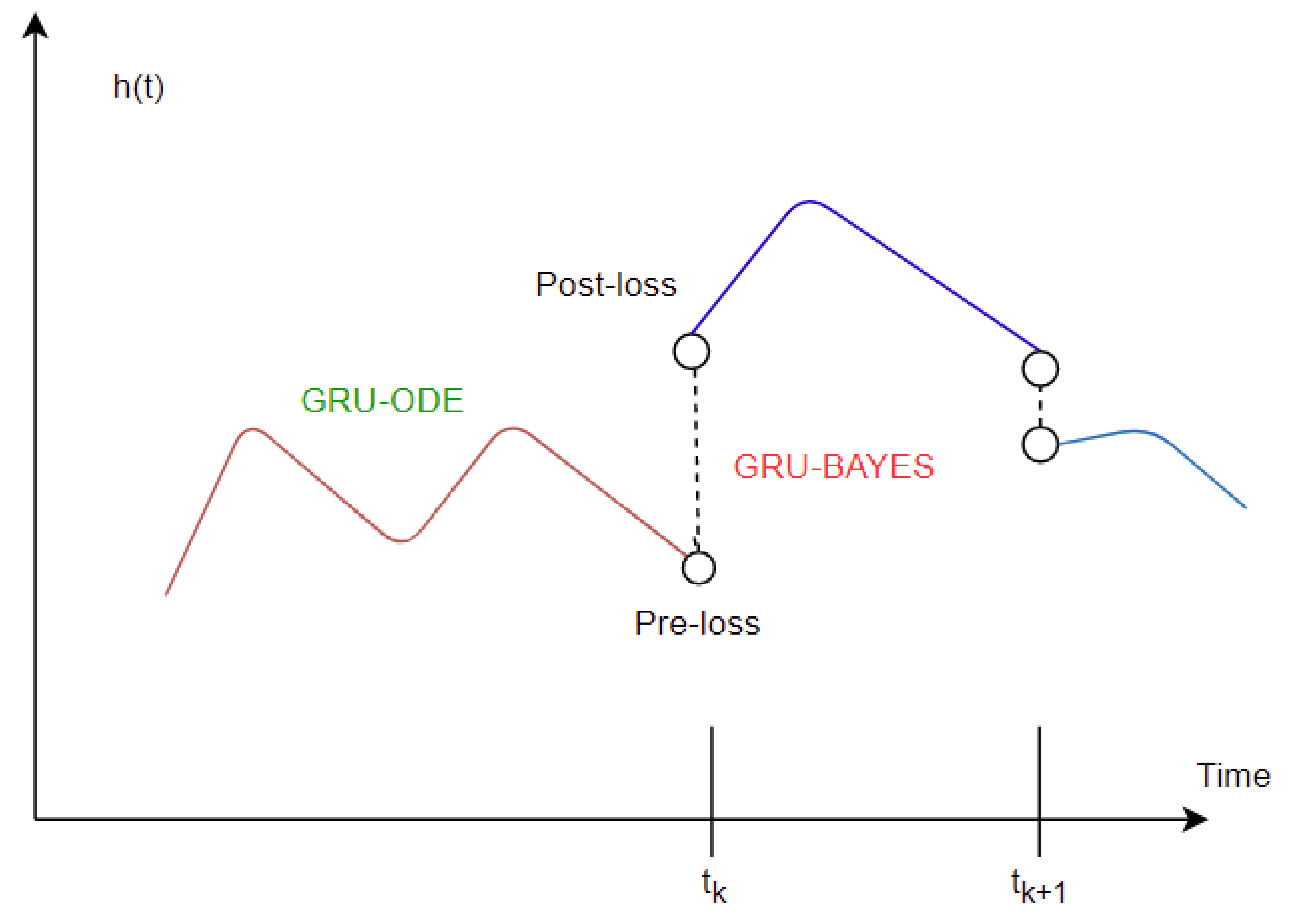
The imputation algorithm presented here is of great importance due to the increasing number of missing values in EHRs. It is very common to have more than 50–60% missing values per channel in EHR time series data. Each patient has some set of demographics, which vary greatly from one patient to the other. Therefore, it is difficult to impute records of one patient based on another. There is hardly any way around this since some patients might not have any measurement for a particular channel or item. As mentioned earlier, the EHR time series data might have some underlying dynamics that might not be approximated well by the stochastic Weiner process. This opens up a great opportunity for further research. As for standard oscillating behaviors, there are many well-established equations to represent the internal dynamics. As shown in many recent articles, the simulated data for standard oscillations can be accurately estimated by the Weiner process. However, this might not be the case for most real-life EHR time series data. The proposed method not only imputes the time series data, but also provides an estimation of the level of uncertainty that the imputed values represent. In the proposed model, the Bayesian estimation is coupled with an LSTM cell. This allows for the update to happen only when there are available values. The missing values are then inferred from the resulting imputed time series. The target is to predict the mean imputed values as close as possible to the actual values. The log variance needs to be smaller as well, since higher levels of uncertainty are much more difficult to propagate and can easily jeopardize the entire predictive model. In most common imputation methods, the mean-squared error is minimized. The proposed method uses two losses (pre and post) before and after Bayesian estimation, which are useful to decide whether the new observational update reduces the error. The two loss functions (negative log likelihood and KL divergence) are well established and widely used in ML techniques. Considering these issues, further research can be concentrated on developing an imputation method that could efficiently learn the dynamics of the underlying process instead of assuming a Weiner process in every case. This would significantly boost performance in complex EHR data.

References

1. Lin, W.C.; Tsai, C.F. Missing value imputation: A review and analysis of the literature (2006–2017). Artif. Intell. Rev. 2019, 53, 1487–1509. [Google Scholar] [CrossRef]
2. Rasmussen, C.E.; Williams, C. Gaussian Processes for Machine Learning, Volume 1; MIT Press: Cambridge, MA, USA, 2006; Volume 39, pp. 40–43. [Google Scholar]
3. Aydilek, I.B.; Arslan, A. A hybrid method for imputation of missing values using optimized fuzzy c-means with support vector regression and a genetic algorithm. Inf. Sci. 2013, 233, 25–35. [Google Scholar] [CrossRef]
4. Iacus, S.M.; Porro, G. Missing data imputation, matching and other applications of random recursive partitioning. Comput. Stat. Data Anal. 2007, 52, 773–789. [Google Scholar] [CrossRef]
5. Armitage, E.G.; Godzien, J.; Alonso-Herranz, V.; López-Gonzálvez, Á.; Barbas, C. Missing value imputation strategies for metabolomics data. Electrophoresis 2015, 36, 3050–3060. [Google Scholar] [CrossRef] [PubMed]
6. Burgette, L.F.; Reiter, J.P. Multiple imputation for missing data via sequential regression trees. Am. J. Epidemiol. 2010, 172, 1070–1076. [Google Scholar] [CrossRef]
7. Nishanth, K.J.; Ravi, V. Probabilistic neural network based categorical data imputation. Neurocomputing 2016, 218, 17–25. [Google Scholar] [CrossRef]
8. Chen, R.T.; Rubanova, Y.; Bettencourt, J.; Duvenaud, D. Neural ordinary differential equations. arXiv 2018, arXiv:1806.07366. [Google Scholar]
9. Rubanova, Y.; Chen, R.T.; Duvenaud, D. Latent odes for irregularly-sampled time series. arXiv 2019, arXiv:1907.03907. [Google Scholar]
10. De Brouwer, E.; Simm, J.; Arany, A.; Moreau, Y. Gru-ode-bayes: Continuous modeling of sporadically-observed time series. arXiv 2019, arXiv:1905.12374. [Google Scholar]
11. Prigogine, I. From being to becoming. Br. J. Philos. Sci. 1982, 33, 325–329. [Google Scholar]
12. Gillespie, D.T. Exact numerical simulation of the Ornstein-Uhlenbeck process and its integral. Phys. Rev. E 1996, 54, 2084. [Google Scholar] [CrossRef] [Green Version]
13. Che, Z.; Purushotham, S.; Cho, K.; Sontag, D.; Liu, Y. Recurrent neural networks for multivariate time series with missing values. Sci. Rep. 2018, 8, 6085. [Google Scholar] [CrossRef] [PubMed] [Green Version]
14. Cho, K.; Van Merriënboer, B.; Gulcehre, C.; Bahdanau, D.; Bougares, F.; Schwenk, H.; Bengio, Y. Learning phrase representations using RNN encoder-decoder for statistical machine translation. arXiv 2014, arXiv:1406.1078. [Google Scholar]
15. Zhou, G.B.; Wu, J.; Zhang, C.L.; Zhou, Z.H. Minimal gated unit for recurrent neural networks. Int. J. Autom. Comput. 2016, 13, 226–234. [Google Scholar] [CrossRef] [Green Version]
16. Cao, W.; Wang, D.; Li, J.; Zhou, H.; Li, L.; Li, Y. Brits: Bidirectional recurrent imputation for time series. arXiv 2018, arXiv:1805.10572. [Google Scholar]
17. Mao, J.; Xu, W.; Yang, Y.; Wang, J.; Huang, Z.; Yuille, A. Deep Captioning with Multimodal Recurrent Neural Networks (m-RNN). arXiv 2014, arXiv:1412.6632. [Google Scholar]
18. Johnson, A.E.; Pollard, T.J.; Shen, L.; Li-Wei, H.L.; Feng, M.; Ghassemi, M.; Moody, B.; Szolovits, P.; Celi, L.A.; Mark, R.G. MIMIC-III, a freely accessible critical care database. Sci. Data 2016, 3, 160035. [Google Scholar] [CrossRef] [Green Version]
19. Dernoncourt, F.; Lee, J.Y.; Uzuner, O.; Szolovits, P. De-identification of patient notes with recurrent neural networks. J. Am. Med. Inform. Assoc. 2017, 24, 596–606. [Google Scholar] [CrossRef] [PubMed]
20. Harutyunyan, H.; Khachatrian, H.; Kale, D.C.; Steeg, G.V.; Galstyan, A. Multitask learning and benchmarking with clinical time series data. arXiv 2017, arXiv:1703.07771. [Google Scholar] [CrossRef] [Green Version]
21. Xue, Y.; Klabjan, D.; Luo, Y. Predicting ICU readmission using grouped physiological and medication trends. Artif. Intell. Med. 2019, 95, 27–37. [Google Scholar] [CrossRef]
22. Anand, V.; Garg, S.K.; Koene, R.; Thenappan, T. National trends in hospital readmission rates in congestive heart failure patients. Circulation 2016, 134, A17286. [Google Scholar]
23. Hoang-Kim, A.; Parpia, C.; Freitas, C.; Austin, P.C.; Ross, H.J.; Wijeysundera, H.C.; Tu, K.; Mak, S.; Farkouh, M.E.; Sun, L.Y.; et al. Readmission rates following heart failure: A scoping review of sex and gender based considerations. BMC Cardiovasc. Disord. 2020, 20, 223. [Google Scholar] [CrossRef]
24. Sundararaman, A.; Ramanathan, S.V.; Thati, R. Novel approach to predict hospital readmissions using feature selection from unstructured data with class imbalance. Big Data Res. 2018, 13, 65–75. [Google Scholar] [CrossRef]
25. Chi, D.J.; Chu, C.C. Artificial Intelligence in Corporate Sustainability: Using LSTM and GRU for Going Concern Prediction. Sustainability 2021, 13, 11631. [Google Scholar] [CrossRef]
26. Shewalkar, A.; Nyavanandi, D.; Ludwig, S.A. Performance evaluation of deep neural networks applied to speech recognition: RNN, LSTM and GRU. J. Artif. Intell. Soft Comput. Res. 2019, 9, 235–245. [Google Scholar] [CrossRef] [Green Version]
Figure 1. Data-cleaning steps.
Biomedinformatics 01 00011 g001
Figure 2. A sample patient time series showing heart rate and arterial blood pressure (diastolic and systolic) measurements.
Biomedinformatics 01 00011 g002
Figure 3. A simple RNN layer.
Biomedinformatics 01 00011 g003
Figure 4. Configuration of a GRU cell.
Biomedinformatics 01 00011 g004
Figure 5. Bayesian jump during the update of hidden layers.
Biomedinformatics 01 00011 g005
Figure 6. GOBI algorithm sequences.
Biomedinformatics 01 00011 g006
Figure 7. Imputation results (heart rate).
Biomedinformatics 01 00011 g007
Figure 8. Imputationresults (systolic blood pressure).
Biomedinformatics 01 00011 g008
Figure 9. Imputationresults (diastolic blood pressure).
Biomedinformatics 01 00011 g009