Machine Learning for Diagnosis of Alzheimer’s Disease and Early Stages

Abstract

According to the WHO, approximately 50 million people worldwide have dementia and there are nearly 10 million new cases every year. Alzheimer’s disease is the most common form of dementia and may contribute to 60–70% of cases. It has been proved that early diagnosis is key to promoting early and optimal management. However, the early stage of dementia is often overlooked and patients are typically diagnosed when the disease progresses to a more advanced stage. The objective of this contribution is to predict Alzheimer’s early stages, not only dementia itself. To carry out this objective, different types of SVM and CNN machine learning classifiers will be used, as well as two different feature selection algorithms: PCA and mRMR. The different experiments and their performance are compared when classifying patients from MRI images. The newness of the experiments conducted in this research includes the wide range of stages that we aim to predict, the processing of all the available information simultaneously and the Segmentation routine implemented in SPM12 for preprocessing. We will make use of multiple slices and consider different parts of the brain to give a more accurate response. Overall, excellent results have been obtained, reaching a maximum F1 score of 0.9979 from the SVM and PCA classifier.

1. Introduction

Wavelet transform [1] and its applications are a powerful tool in image processing. Since the rise of wavelet analysis in the early 1980s, it has been shown to be useful in many fields of applied mathematics, specifically in signal and image processing.

The recent advances in neural networks and transfer learning methods [2] have opened the door to discussions about the goodness and supremacy of neural networks over the traditional transforms in pattern recognition and classification.

At the same time, Alzheimer’s disease has established itself as one of the great epidemics of the 21st century, being the most common case of dementia. It has been proved to present intermediate stages before the severity of the dementia becomes moderate or serious. These stages can be noticeable and, on occasion, patients are even aware of their own cognitive impairment. However, such symptoms can go unnoticed until the disease presents an advanced stage. Detecting and diagnosing early stages can be the key to provide patients with better prognosis and preventive treatments in order to improve their quality of life.

The latest experiments were able to find a correlation between the information contained in brain MRI images and the presence of dementia. These experiments made use of a wide variety of methods and algorithms. The first investigations were based mainly on traditional transforms [3] and VBM plus DARTEL analysis [4] techniques for feature extraction and state of the art Support Vector Machine (SVM) classifiers. Generally, these experiments obtained good results (92.36% and 96.32% accuracy respectively) classifying binary (Alzheimerś disease (AD) and control (CN)) stages.

In the last five years, more stages of the disease, including mild cognitive impairment (MCI), have been included in the classification and neural networks have gradually assumed greater importance. These classifiers normally outperformed previous accuracies, as stated in [5] (97.50%), [6] (97.51%), or [7] (99.1%). By combining them with other techniques such as latent transition analysis [8] it is possible to predict status changes in Alzheimer’s disease. For this investigation, the line of research proposed by [9,10] will be followed. In particular, we will make use of the Segmentation routine implemented in SPM12 [11,12] for preprocessing and the most relevant volumes of the brain related to Alzheimer’s disease discovered in [10].

This research will thoroughly analyze the full content of the MRI images and contrast them again the afore-mentioned experiments, aiming to predict up to six different stages of dementia. The objective is to use the nine best slices proposed in [10] and simultaneously apply two different approaches as suggested in [13,14]: two-dimensional multiresolution analysis (2-D MRA) in $L^2\left({\mathbb{R}}^2\right)$, aligned with SVM and convolutional neural network (CNN) [15,16].

Following, also, the strategy used in [10,17], the mRMR algorithm will be used to extract the coefficients to feed the SVM classifier. Subsequently, its performance will be contrasted with the traditional PCA algorithm.

Overall, this research aims to answer to several questions. First, whether it is possible to predict and prevent the appearance of the Alzheimer’s disease, considering up to six stages of dementia: cognitively normal, significant memory concern, early mild cognitive impairment, mild cognitive impairment, late mild cognitive impairment, and Alzheimer’s disease. Secondly, which of the aforementioned algorithms performs better after the application of SMP12 preprocessing? Thirdly, what is the result of processing multiple slices in conjunction instead of using single slices for classification? Lastly, how to address the problem of memory management when using larger volumes of information for model training.

2. Materials and Methods

One of the key points is to decide which of the following algorithms performs better when detecting Alzheimer’s disease from MRI images: SVM or CNN. An additional experiment will be conducted using transfer learning based on VGG16, a convolutional neural network model proposed by K. Simonyan and A. Zisserman, from the University of Oxford, in the paper “Very Deep Convolutional Networks for Large-Scale Image Recognition”. Similar transfer learning approaches were suggested in [6]. Another key point is to learn the best strategy to use in terms of data handling. By example, we will address the question of whether it is better to process a single slice at a higher level of detail or to process, simultaneously, more than one slice with at lower level thereof. Additionally, we need to determine the classes that are of most importance. It is evident that the sooner the disease is detected, the better the prognosis will be for the patient. It will be also relevant for us to test the model’s performance in detecting Alzheimer’s in its early stages. Restrictions apply to the availability of this data. Data was obtained from http://adni.loni.usc.edu (accessed on 20 May 2020), and is available with the permission of The Alzheimer’s Disease Neuroimaging Initiative (ADNI). The primary goal of ADNI has been to test whether serial magnetic resonance imaging (MRI), positron emission tomography (PET), other biological markers, and clinical and neuropsychological assessment can be combined to measure the progression of mild cognitive impairment (MCI) and early Alzheimer’s disease (AD). The complete database of ADNI including ADNI1, ADNI-GO, ADNI2 and ADNI3, are used for this investigation. The set downloaded comprises brain images in NIfTI (Neuroimaging Informatics Technology Initiative) format. Corrupt and duplicated images were deleted, resulting in a total of 6028 T1-weighted MRI images. The methodology described in [9,10] is used for the pre-processing of the information from the sample data. This pre-processing, which requires segmentation, bias correction and spatially normalisation, has been performed using the Segmentation routine implemented in SPM12 [11,12]. The number of samples in the data constitutes a considerable improvement to [9,10], where 400 and 242 images were obtained, respectively. The full project and code are available on https://github.com/juliopradom/alzheimer-classifier (accessed on 6 December 2021).

2.1. Problem Exploration

As mentioned before, the set of images provided are classified into six groups:

• AD (Alzheimer Disease): the images in this group correspond to patients diagnosed with Alzheimer.
• CN (Cognitively Normal): corresponds to healthy individuals (control).
• MCI (Mild Cognitive Impairment): causes a slight but noticeable and measurable decline in cognitive abilities.
• EMCI (Early Mild Cognitive Impairment): an early stage of MCI with milder episodic memory impairment.
• LMCI (Late Mild Cognitive Impairment): a more advanced stage of MCI previous to AD.
• SMC (Significant Memory Concern): patients with SMC are characterized by self-report significant memory concern, quantified by using the Cognitive Change Index and the Clinical Dementia Rating (CDR) of zero. SMC participants score within the normal range for cognition, and the informant does not equate the expressed concern with progressive memory impairment. SMCs have been shown to be correlated with a higher likelihood of progression [18].

With these classes, we can build a progression diagram for Alzheimer’s disease, as shown in Figure 1.

Unlike other experiments and investigations, by achieving the goals set for this classifier we will not only discern between healthy patients and patients with dementia but also provide a more accurate diagnosis about the stage of their dementia. This may be useful to detect the disease earlier and prescribe a more effective and personalized treatment to those individuals situated in intermediate stages.

By looking at Figure 2 we can observe the number of samples per category. LMCI, MCI, AD and CN have approximately the same number of samples (∼1200) whereas SMC and EMCI are clearly unbalanced. Particular attention is paid to these minority classes given that, as commented upon at the beginning of this chapter, our specific focus is on Alzheimer’s early stages.

Each of the samples is composed of nine different images corresponding to nine different slices from an MRI image. Slices 55, 56, 61, 72, 82, 90, 104, 106 and 114 are used, according to the most promising slices obtained in [10], after the application of multi-objective genetic algorithms to find most relevant volumes of the brain related to Alzheimer’s disease and mild cognitive impairment.

The images have three different colour channels (RGB) and are already resized to $656\times 875$. As a result, every image is an array with shape $(656,875,3)$. In Figure 3 shows the nine images for patient 1 in AD.

In practice, the management of all this information is very resource-consuming. This will be a limiting factor throughout our investigation. Smart approaches must be taken to overcome these obstacles and will be covered in depth in the following sections.

Having analysed and described our data, two lines of research are going to be opened. First, we are going to proceed to extract and select features with which to apply SVM. Secondly, we will use a custom CNN and CNN with transfer learning to train our model without further preprocessing.

Global F1 (macro) is the measurement that we will use to compare the performance of the different algorithms. However, it is essential to remember that another relevant indicator that we will use in practice, when facing similar scores, is the specific performance (F1) of the algorithms identifying SMC and EMCI.

2.2. SVM Research

Building a support vector machine classifier using wavelet coefficients extracted from our images is the first approach. By using wavelet coefficients, the identification of relevant anomalies and slight changes within our samples will be easily detected, which is, actually, what we are seeking to achieve in distinguishing between one class or another.

The coefficients extracted for a given patient can be used to construct a vector in a high-dimensional space. The set of these vectors labelled with their corresponding classes will help determine a hyperplane able to separate each group from the other. In practice, one hyperplane will be created for every class. This research is carried out using the scikit-learn library.

For our experiment, only the wavelet coefficients of the approximation image at level three and four are accessed for memory reason. It is mandatory to first convert the images from RGB space to grey so the wavelet module used can extract the coefficients using a single channel. In particular, we will perform ten extractions; one for every slice available and one combining all the coefficients consecutively. Extracting one slice means obtaining the wavelet coefficients at the third level for every patient at this specific slice, which gives a total of 6028 arrays of 10,120 coefficients each. Extracting all the coefficients means obtaining the wavelet coefficients at the fourth level for all the available slices and combine them, which, again, gives a total of 6028 arrays of 9 × 2867 = 25,803 coefficients each. In

Table 1. Number of wavelet coefficients per image for some approximation levels. The lower the level we access, the better the image can be reconstructed. Levels higher than five are not relevant for this investigation and therefore are not included.

Level 5	Level 4	Level 3	Level 2	Level 1
918	2867	10,120	37,856	145,971

are shown some of the coefficients we could extract per image.

Nevertheless, as previously mentioned, going beyond the third level becomes computationally difficult for the machine used in our research. For such purpose, mini-batch training techniques must be used, which is beyond the objectives of this investigation. Sensitive information loss could be a possible consequence to this limitation, which could result in a worse F1 performance. After the coefficients are successfully extracted, it is important to note that we have arrays of 10,120 and 25,803 coefficients, respectively. In order to generate an input small and meaningful enough to train and work with our models it is necessary to apply feature selection. For this objective, we will perform two different experiments using two methods: mRMR (as used in [7,10,19]) and the traditional PCA.

mRMR is an iterative algorithm that starts with an empty set S, and for each iteration searches for an input feature p that maximizes the mutual information (MI) [20,21] with respect to the output feature. After this, it minimizes MI with respect to the rest of input features, that is, maximizes the relevance and minimizes the redundancy. This feature is added to S. The algorithm finishes when all features are added. Moreover, the final ranking is the order in which they have been added to S. On the other hand, principal component analysis (PCA) [22] is another technique for reducing the number of variables in the sample data. However, unlike mRMR, this algorithm does not preserve the original features, but it applies dimensionality reduction. The objective of PCA is to transform the original random vector into variables called principal components. These components are all orthogonal and ordered so that the first few explain most of the variation of the random vector. PCA is a widely used algorithm for feature selection. Given the interest and good results [7,10,19] provided by mRMR, this research finds it appropriate to compare how both techniques affect the outcome of the classification.

For the first experiment, mRMR is used to select the best 100 coefficients. This algorithm is extremely resource consuming and it is not possible to pass the whole set of arrays at once. In order to overcome this issue, a recursive version of this algorithm was designed and built. Both recursive and original versions have been tested on a small set of 100 features, obtaining a similar set of features, as expected (maximum relevance and minimum redundancy principle). The functioning of this recursive version is shown in Figure 4.

It is worth noting that the application of mRMR will give a set of existent features as a result. Before starting the process, the data is standardized and rescaled in order for the mean of the observed values to be 0 and the standard deviation to be 1. This can be particularly practical in avoiding different scales between our images and to take a step further to ensure normalization.

The same process is repeated, but using PCA this time. Contrary to mRMR, using PCA we obtain 100 new features as a result of dimensionality reduction; that is, we keep the information of all the original features in a smaller set. No particular considerations needs to be taken to perform PCA as the module used is powerful enough to be utilized with an input of our size.

The next step is to find the best hyperparameters with which to tune our SVM model. After applying a grid search using slice 55 on the set of hypermarameters, as shown in

Table 2. Hyperparameter space considered for SVM. A total of $3\times 4\times 5=60$ combinations are tested when applying a grid search. This number corresponds to all the possible combinations between kernels, C and gamma parameters.

Kernel	C	Gamma
linear, rbf, sigmoid	1, 10, 100, 1000	${10}^{-1}$, ${10}^{-2}$, ${10}^{-3}$, ${10}^{-4}$, scale

, considering that C is the regularization parameter and gamma is the kernel coefficient, the most promising hyperparameters using the output of mRMR are $\mathrm{kernel}=\mathrm{rbf}$, $C=1000$ and $gamma={10}^{-2}$. Correspondingly, using the output of PCA we obtain the parameters $\mathrm{kernel}=\mathrm{rbf}$, $C=10$ and $gamma=\mathrm{scale}$.

Following [23], when creating the SVM, the strategy to use will be one-against-one since our kernel is based on a radial basis function (rbf). In all the experiments conducted the set of patients is split into training and test sets. These sets will remain unchanged to contrast the results more effectively. Specifically, the training set covers 75% (4521) of the available samples and test set covers the rest 25% (1507), where the number of representatives for each class follows the original distribution in both sets. In addition, the number 104,729 is used as a random seed for shuffling. The pre-processing and classification pipeline is summarized in Figure 5.

2.3. CNN Research

The second part in our investigation is to train a convolutional neural network using, directly, the images available as input. Along with a custom CNN, we will also test VGG16, modifying the input and output layers. For both experiments, the number of epochs is set to 500 and the images are resized to $224\times 224$ according to VGG16’s requirements. The objective is to make both experiments as similar as possible.

By using CNN, the pre-processing steps covered in SVM can be skipped, since CNN is able to learn features from the image itself. Additionally, we can keep the RGB channels to make our input a tensor of order four. In order to be able to compare the performance of CNN with SVM, the same training and test set are considered. To construct our networks TensorFlow is used on a cluster containing two GPUs NVIDIA RTX 2080.

To build our CNN, we perform two experiments with two common and effective structures consisting of the following sequence of layers:

Experiment 1:

1.

One convolutional layer with 32 filters, a kernel size of (3,3) and using “relu” as its activation function. The number of filters determines the number of kernels to convolve with the input volume. Each of these operations produces a 2D activation map. Layers early in the network architecture (i.e., closer to the actual input image) usually learn fewer convolutional filters while layers deeper in the network (i.e., closer to the output predictions) will learn more filters. This layer will expect an input of size (224, 224, 3) in order to fit our images.

2.

One max pooling layer (2,2) to reduce the spatial dimensions of the output volume.

3.

Another similar convolutional layer, although using 64 filters this time.

4.

Another max pooling layer (2,2) to reduce the spatial dimensions of the output volume in the second convolutional layer.

5.

One flattened layer to connect the multidimensional data from convolution to dense layers.

6.

Two dense layers using the “relu” (64 units) and “softmax” (6 units) activation functions respectively. We use “softmax” to convert the scores to a normalized probability distribution.

Experiment 2:

1.

One convolutional layer with 16 filters, a kernel size of (3,3) and using “relu” as its activation function.

2.

One max pooling layer (2,2) to reduce the spatial dimensions of the output volume.

3.

Another similar convolutional layer, but using 32 filters this time.

4.

Another max pooling layer (2,2) to reduce the spatial dimensions of the output volume in the second convolutional layer

5.

A third convolutional layer but using 64 filters.

6.

A third max pooling layer (2,2) to reduce the spatial dimensions of the output volume in the third convolutional layer.

7.

One flatten layer to connect the multidimensional data from convolution to dense layers.

8.

Two dense layers using the “relu” (128 units) and “softmax” (6 units) activation functions respectively. We use “softmax” to convert the scores to a normalized probability distribution.

Both experiments will process 500 epochs. Replicating the experiments conducted in SVM, we build a model for every slice. Again, the training set covers 75% (4521) of the available samples and the test set covers the remaining 25% (1507), where the number of representatives for each class follows the original distribution in both sets. In addition, the number 104,729 is used as random seed for shuffling.

3. Results

3.1. SVM Results

Let us now begin analysing the results from the mRMR tests, in which our main objective is to maximize F1 score. Looking at

Table 3. F1 results for SVM combined with mRMR. In the table we can see the performance of each slice when predicting specific stages. The average score is included on the right side. The all-coefficients classifier obtains the highest F1 score, 0.9657. The best single-slice classifier corresponds with slice 82.

	CN	SMC	EMCI	MCI	LMCI	AD	Average
55	0.8090	1	1	1	1	0.8148	0.9373
56	0.8007	1	1	1	1	0.8133	0.9361
61	0.8083	1	1	1	1	0.8122	0.9367
72	0.7958	1	1	1	1	0.8040	0.9333
82	0.8091	1	1	1	1	0.8180	0.9379
90	0.7917	1	1	1	1	0.7980	0.9316
104	0.7825	1	1	1	1	0.7933	0.9293
106	0.7813	1	1	1	1	0.7706	0.9253
114	0.8035	1	1	1	1	0.8101	0.9356
All	0.8909	1	1	1	1	0.9032	0.9657

, we can observe that the results obtained are decent. Classes in the middle are perfectly recognized and predicted, whereas control and sick patients present an observably worse score. The experiment with the best results is the one that used all the available coefficients at level four. This result is of interest since it shows that processing all the information as a whole is, in principle, more effective than using single slices for classification, even if the level of detail accessed is lower.

In Figure 6 we can see more distinctly see the different scores between slices. After this experiment we have reached an F1 score of 0.9657. Regarding the models built using single slices, we can see that slice 82 slightly stands out from the rest. Below we will discuss if this trend is confirmed.

The same experiment was reproduced using PCA, as shown in

Table 4. F1 results for SVM combined with PCA. In the table we can see the performance of every slice when predicting specific stages. The average score is included on the right side. The all-coefficients classifier obtains the highest F1 score, 0.9979. The best single-slice classifiers correspond to slices 104 and 106.

	CN	SMC	EMCI	MCI	LMCI	AD	Average
55	0.9912	0.9939	1	0.9984	0.9930	0.9917	0.9947
56	0.9930	0.9939	1	0.9984	0.9930	0.9933	0.9953
61	0.9947	0.9939	0.9896	0.9984	0.9903	0.9950	0.9936
72	0.9947	0.9939	0.9948	1	0.9930	0.9950	0.9952
82	0.9912	1	1	1	0.9958	0.9933	0.9967
90	0.9947	1	0.9948	1	0.9944	0.9967	0.9968
104	0.9947	1	1	0.9984	0.9958	0.9950	0.9973
106	0.9947	1	1	0.9984	0.9958	0.9950	0.9973
114	0.9947	1	0.9948	1	0.9944	0.9967	0.9968
All	0.9947	1	1	1	0.9958	0.9967	0.9979
Multi-Slice	0.9930	1	1	1	0.9958	0.9950	0.9973

. We not that it is undeniable how well the classifier performed when using PCA for every slice. This time the slices with the best results were slices 104 and 106. As the method performed to extract the coefficients (PCA) transformed and resized all the available information, we could build the following hypothesis, considering, also, the conclusions from mRMR: slice 82 is the most informative slice when looking at specific regions of the image but slices 104 and 106 are more relevant when viewing the image as a whole. Again, the experiment with the best outcome continues to be the all-coefficients classifier, with an outstanding F1 score, in this case, of 0.9979.

An extra experiment was conducted, also using PCA, and was noted as “Multi-Slice”. This test retrieves the output of every slice and selects the most common value, simulating a decision system between different experts, as shown in Figure 7. It is not a model in and of itself; rather, it applies the mode of the single-slice models.

However, the all-slices classifier performs better, confirming the hypothesis opened after discussing the results from mRMR: processing all the information is more effective than focusing on specific areas. A visual representation of the scores for the different slices using PCA is shown in Figure 8.

Thus far, our classifier is able to recognize SMC, EMCI and MCI perfectly. We will contrast the score obtained from the all-slices classifier against the outcome of CNN in the following section. By using PCA we have achieved an increment of more than 3% in F1 score, as shown in Figure 9. It is also notable that this approach provides a most homogeneous performance for every slice.

3.2. CNN Results

The pattern observed in the previous section is repeated, using, now, CNN. Slices 104 and 106 are the most informative (although slice 72 was the most relevant in Experiment 2) and SMC, EMCI, MCI and LMCI are nearly perfectly matched, with a noticeable but not pronounced difficulty identifying CN and AD (See

Table 5. F1 results for custom CNN, Experiment 1. In the table we can see the performance of every slice when predicting specific stages. The average score is included on the right side. The multi-slice classifier obtains the highest F1 score, 0.9902. The best single-slice classifier correspond to slices 104 and 106.

	CN	SMC	EMCI	MCI	LMCI	AD	Average
55	0.9683	1	1	1	1	0.9701	0.9897
56	0.9682	1	1	1	1	0.9702	0.9897
61	0.9665	1	1	1	1	0.9685	0.9892
72	0.9652	1	1	1	1	0.9641	0.9873
82	0.9648	1	1	1	1	0.9668	0.9886
90	0.9686	1	1	1	1	0.9657	0.9879
104	0.9686	1	1	1	1	0.9698	0.9897
106	0.9700	1	1	1	1	0.9718	0.9903
114	0.9628	1	0.9984	1	1	0.9669	0.9880
Multi-Slice	0.9699	1	1	1	1	0.9709	0.9902

and

Table 6. F1 results for custom CNN, Experiment 2. In the table we can see how every slice performs when predicting specific stages. The average score is included on the right side. Multi-Slice classifier obtains the highest F1 score along with slice 72, 0.9902.

	CN	SMC	EMCI	MCI	LMCI	AD	Average
55	0.9385	1	1	1	1	0.9418	0.9800
56	0.9370	1	1	1	1	0.9399	0.9784
61	0.9338	1	0.9984	1	1	0.9377	0.9783
72	0.9561	1	1	1	1	0.9584	0.9857
82	0.9422	1	1	1	1	0.9449	0.9812
90	0.9439	1	1	1	1	0.9467	0.9818
104	0.9537	1	1	1	1	0.9572	0.9852
106	0.9521	1	1	1	1	0.9574	0.9850
114	0.9345	1	1	1	1	0.9388	0.9789
Multi-Slice	0.9563	1	1	1	1	0.9582	0.9857

).

The “multi-slice” aggregator (see previous section) is also included and performs better than considering the decision of every slice separately, reaching a maximum F1 score of 0.9902. Note that, for CNN, it is not possible to build the all-slices classifier because the input of our model would be too large for the machine on which this research was carried out.

Despite the fact that the scores obtained using the custom CNN are more than adequate, it still performs worse than our SVM classifier based on PCA (recognising that we acheived an F1 of 0.9979 with this classifier)). In Figure 10 and Figure 11 we examine the final score for each slice and experiment.

For the last experiment, we will use the VGG16 pre-trained model with a custom output (dense) layer using, again, “softmax” as the activation function. This model requires a longer time to train, since the number of layers and weights are significantly higher than in our custom CNN. Jumping directly into the results in

Table 7. F1 results for CNN using transfer learning. In the table we can see the performance of every slice when predicting specific stages. The average score is included on the right side. The multi-slice classifier obtains the maximum F1 score, 0.9620. It is closely followed by slice 56, which reaches an F1 score of 0.9618.

	CN	SMC	EMCI	MCI	LMCI	AD	Average
55	0.8730	1	1	1	1	0.8773	0.9584
56	0.8839	1	1	1	1	0.8870	0.9618
61	0.8801	1	1	1	1	0.8758	0.9569
72	0.8731	1	1	1	1	0.8770	0.9583
82	0.8728	1	1	1	1	0.8808	0.9589
90	0.8667	1	0.9984	1	1	0.8752	0.9567
104	0.8785	1	0.9967	1	1	0.8826	0.9596
106	0.8662	1	1	1	1	0.8738	0.9567
114	0.8723	1	0.9984	1	1	0.8797	0.9584
Multi-Slice	0.8841	1	1	1	1	0.8873	0.9620

, we can see that the previous pattern is not repeated: slice 56 is the best classifier. This is most likely due to easier recognition patterns present in slice 56 for VGG16. The highest score obtained belongs to “multi-slice” classifier as expected, with a total F1 score of 0.9620.

It would be interesting to compare the results obtained from VGG16 with those outputted from other transfer learning models such as ResNet50, Inceptionv3 or EfficientNe. Although the preprocessing and training parts differ from the experiments conducted in [6], VGG16 can take second place between the pretrained models used in the previous classification. Nevertheless, this extension goes beyond the objective of this investigation. With respect to VGG16, a more pronounced difference in terms of performance is detectable between the slices (see Figure 12).

Overall, the classifier performs very well. However, once we have covered all the possible approaches, the tested transfer learning solution proves not to be the best option between the available CNN alternatives, as shown in Figure 13.

3.3. Confusion Matrix

Finally, it is worth including the confusion matrix for the best classifier i.e., the confusion matrix for the SVM all-coefficients model. As shown in Figure 14, three out of the four wrong predictions were false LMCI negatives. This implies that the model can eventually make a wrong prediction when dealing with patients in advanced stages of the disease.

It is worth noting that the accuracy score is 0.9973. This will be insightful in comparing the proposed classifier with previous investigations.

4. Discussion and Conclusions

The development of this work was motivated not only by medical purposes but also for the non-unified criteria regarding the usage of support vector machine and convolutional neural networks. Progressively, medicine and artificial intelligence tend to operate together and are proving to obtain outstanding results with respect to enhancing people’s lives. The limits of this symbiosis are still uncertain, although it seems undeniable that, from such combination, we are entering a new era in science, here, early in the 21st century.

Considering our results, the following conclusions can be highlighted:

• It is possible to detect the early stages in Alzheimer’s disease and this prediction can be as precise as the prediction of dementia itself. Significant memory concern (SMC) and early mild cognitive impairment (EMCI) have been proven to have an effect on the brain that can be detected and measured. Patients with early symptoms of dementia can be localized and preventive treatments can be applied.
• If the MRI images reach a high level of normalization and enough samples are accessible it is possible to build an SVM classifier able to predict Alzheimer’s stages with an F1 score higher than 99.7%. As mention throughout the research, a key point of this investigation is the high quality of the dataset and the segmentation, bias correction and spatial normalisation applied by SPM12 [11,12] beforehand. The large number of samples (6,028) used it also relevant when compared with similar investigations [10]. The results show that our model has outperformed other modern experiments [5,6,7,14,24,25]. A more detailed comparison with some of the most promising investigations conducted to date is made in

  Table 8. More detailed comparison between recent relevant investigations. Some experiments have already passed the accuracy threshold of 0.99. The proposed method exceeds this threshold (0.997) and includes six different stages in its classification.

  Authors	Imaging	Stages	Preprocessing	Classifier	Accuracy
  Beheshti et al., 2016 [4]	MRI	CN, AD	VBM plus DARTEL	PCA + SVM	0.963
  You et al., 2020 [25]	EGG	CN, MCI, AD	ASTGCN	ASTGCN	0.910
  AbdulAzeem et al., 2021 [5]	MRI	CN, MCI, AD	Grey scale conversion + Adaptative Thresholding	CNN	0.975
  Eroglu et al., 2021 [7]	MRI	CN, MCI, AD	CNN(TL)	mRMR + SVM	0.991
  Valenzuela et al., 2018 [10]	MRI	CN, MCInc, MCIc, AD	SMP12	PCA + SVM	0.944
  Proposed method	MRI	CN, SMC, EMCI, MCI, LMCI, AD	SPM12 + standardization	PCA + SVM	0.997

  .
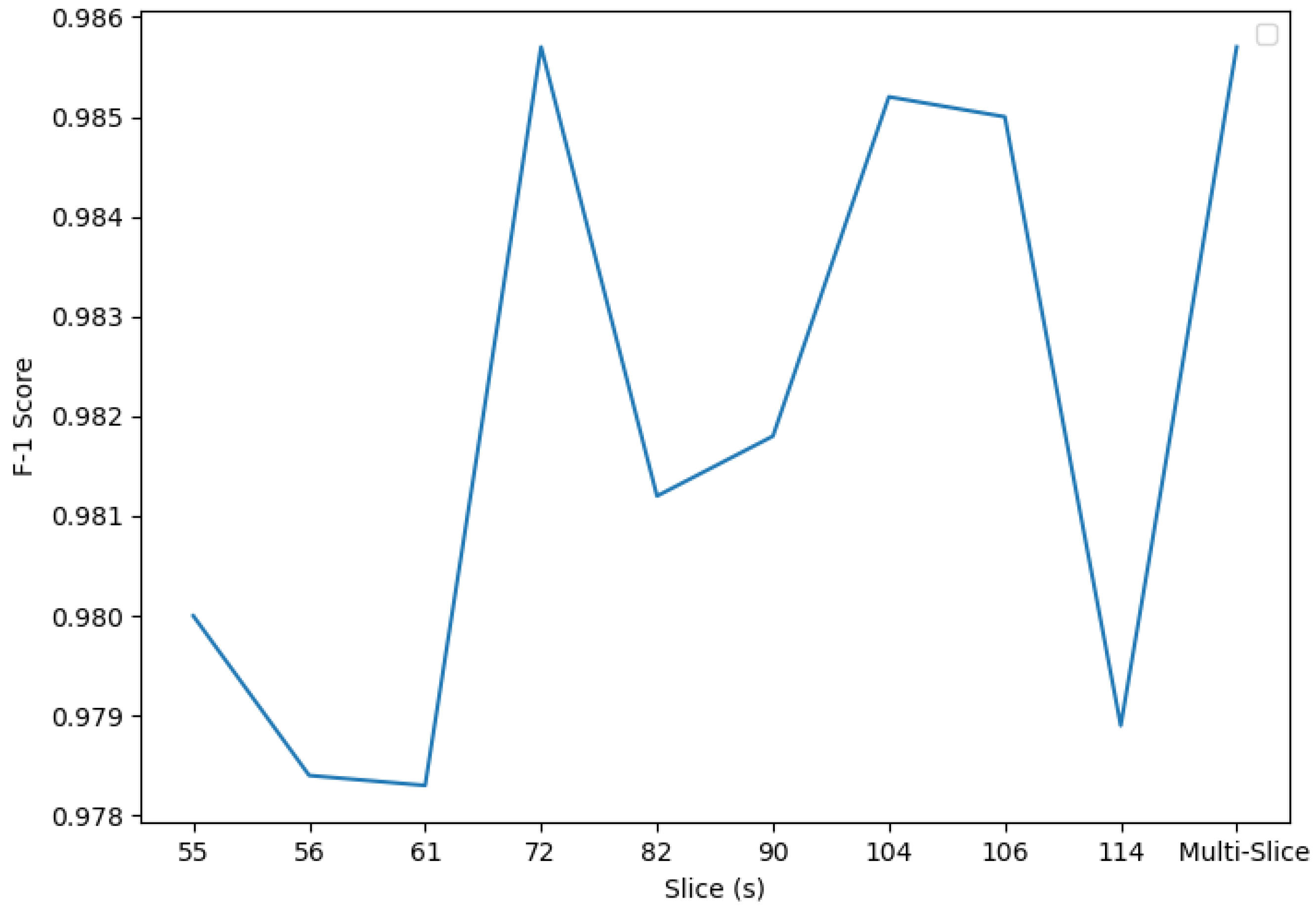
• In MRI images, some slices are more informative than others i.e., there are parts in the brain that contain more information and can be used more precisely to provide a diagnosis of the patient. Of the available slices in our dataset, slice 82 demonstrated the best results. This slice is located in the coronal plane, confirming the conclusions exposed by Luis Balderas in his thesis [9].
• In order to give a more accurate diagnosis, it is better to process all the information available in the brain rather than considering located regions only. Even if the disease has a more noticeable impact on specific regions, the information distributed throughout the brain’s mass makes a difference when seeking optimal results.
• Both SVM and CNN approached competent performances. Nevertheless, SVM stands out above CNN. A possible explanation for this is the normalization and regularity of the data. Since the available images are already resized, and the classifier is built using delimited and localized variation of the imaged zones, the edge identification power of CNN does not beat the capacity of SVM to allocate samples in ${\mathbb{R}}^n$, $n\in \mathbb{N}$ and group them using the partitions generated by its trained hyperplane.
• The Mallat algorithm, revealed in [26], can be used to access the wavelet coefficients at deeper levels of the approximation image, LL. These coefficients are still very informative, exposing the power of the wavelet transform even in today’s image classification tasks. Using the wavelet coefficients from the approximation image at level four gave an outstanding F1 score of 0.9979. This classifier, which used all the available coefficients from the set of slices, performed better than slice-isolated classifiers accessing wavelet coefficients at level three.
• PCA performs better than regular feature selection algorithms when facing image classification problems where data has certain continuity properties. Features are highly correlated with each other and present small variations. Applying feature selection could lead to missing wider anomalies that would otherwise be detected using a dimensionality reduction system.

Disease’s diagnosis using MRI is an open and extensive line of research. To continue and improve the steps followed in this investigation, I suggest these possible lines:

• It would be possible to access a higher level of detail either by using a machine with better specifications or performing mini-batch training techniques. This approach could lead to obtaining a more informative training dataset. Examples of this include using wavelet coefficients at lower levels or training a CNN classifier using all the available images as input.
• Investigate whether accessing different types of wavelet coefficients (diagonal, horizontal or vertical) can lead to a better outcome in F1 score or not.
• Research on the structure of CNN models to develop smarter and more suitable networks using different distribution and types of convolutional layers.
• Develop new paradigms of research to process 3D images and investigate the possible use and applications of the 3D wavelet transform.

References

1. Tan, Y. Continuous Wavelet Transforms. In Wavelet Theory Approach to Pattern Recognition; Bunke, H., Wang, P.S.P., Eds.; World Scientific Publishing Co. Pte. Ltd.: Singapore, 2009; pp. 75–102. [Google Scholar]
2. Iqbal, M.S.; Ahmad, I.; Khan, T.; Khan, S.; Ahmad, M.; Wang, L. Recent Advances of Deep Learning in Biology. In Deep Learning for Unmanned Systems; Koubaa, A., Azar, A.T., Eds.; Studies in Computational Intelligence; Springer: Cham, Switzerland, 2021; Volume 984. [Google Scholar]
3. Zhang, Y.; Dong, Z.; Phillips, P.; Wang, S.; Ji, G.; Yang, J.; Yuan, T. Detection of subjects and brain regions related to Alzheimer’s disease using 3D MRI scans based on eigenbrain and machine learning. Front. Comput. Neurosci. 2015, 9, 66. [Google Scholar] [CrossRef] [PubMed] [Green Version]
4. Beheshti, I.; Demirel, H. Feature-ranking-based Alzheimer’s disease classification from structural MRI. Magn. Reson. Imaging 2016, 34, 252–263. [Google Scholar] [CrossRef] [PubMed]
5. AbdulAzeem, Y.; Bahgat, W.; Badawy, M. A CNN based framework for classification of Alzheimer’s disease. Neural Comput. Appl. 2021, 33, 10415–10428. [Google Scholar] [CrossRef]
6. Shanmugam, J.; Duraisamy, B.; Simon, B.; Bhaskaran, P. Alzheimer’s disease classification using pre-trained deep networks. Biomed. Signal Process. Control 2022, 71, 103217. [Google Scholar] [CrossRef]
7. Eroglu, Y.; Yildirim, M.; Cinar, A. mRMR-based hybrid convolutional neural network model for classification of Alzheimer’s disease on brain magnetic resonance images. Int. J. Imaging Syst. Technol. 2021. [Google Scholar] [CrossRef]
8. Alashwal, H.; Diallo, T.; Tindle, R.; Moustafa, A. Latent Class and Transition Analysis of Alzheimer’s Disease Data. Front. Comput. Sci. 2020, 2, 1–13. [Google Scholar] [CrossRef]
9. Balderas, L. Development of Intelligent System for the automatic classification of Parkinson’s Disease Using MRI Images. Diploma Thesis, University of Granada, Granada, Spain, 2019. [Google Scholar]
10. Valenzuela, O.; Jiang, X.; Carrillo, A.; Rojas, I. Multi-Objective Genetic Algorithms to Find Most Relevant Volumes of the Brain Related to Alzheimer’s Disease and Mild Cognitive Impairment. Int. J. Neural Syst. 2018, 28, 1850022. [Google Scholar] [CrossRef] [PubMed]
11. Penny, W.; Friston, K.J.; Ashburner, J.T.; Kiebel, S.J.; Nichols, T.E. Statistical Parametric Mapping: The Analysis of Functional Brain Images; Academic Press: San Diego, CA, USA, 2007. [Google Scholar]
12. Flandin, G.; Friston, K.; Carrillo, A.; Rojas, I. Analysis of family-wise error rates in statistical parametric mapping using random field theory. Hum. Brain Mapp. 2017, 40, 2052–2054. [Google Scholar] [CrossRef] [PubMed]
13. Hasan, H.; Shafri, H.; Habshi, M. A Comparison Between Support Vector Machine (SVM) and Convolutional Neural Network (CNN) Models For Hyperspectral Image Classification. IOP Conf. Ser. Earth Environ. Sci. 2019, 357, 012035. [Google Scholar] [CrossRef] [Green Version]
14. Buvaneswari, P.; Gayathri, R. Detection and Classification of Alzheimer’s disease from cognitive impairment with resting-state fMRI. Neural Comput. Appl. 2021. [Google Scholar] [CrossRef]
15. Khan, S.; Rahmani, H.; Afaq, S.; Shah, A.; Bennamoun, M. Convolutional Neural Network. In A Guide to Convolutional Neural Networks for Computer Vision; Medioni, G., Dickinson, S., Eds.; Morgan & Claypool Publishers: San Rafael, CA, USA, 2018; pp. 43–95. [Google Scholar]
16. Khan, S.; Rahmani, H.; Afaq, S.; Shah, A.; Bennamoun, M. Examples of CNN Architectures. In A Guide to Convolutional Neural Networks for Computer Vision; Medioni, G., Dickinson, S., Eds.; Morgan & Claypool Publishers: San Rafael, CA, USA, 2018; p. 104. [Google Scholar]
17. Logan, R.; Williams, B.; da Silva, M.; Indani, A.; Schcolnicov, N.; Ganguly, A.; Miller, S. Deep Convolutional Neural Networks With Ensemble Learning and Generative Adversarial Networks for Alzheimer’s Disease Image Data Classification. Front. Aging Neurosci. 2021, 13, 720226. [Google Scholar] [CrossRef]
18. The Alzheimer’s Disease Neuroimaging Initiative. Available online: http://adni.loni.usc.edu/study-design/ (accessed on 20 May 2020).
19. Billah, M.; Waheed, S. Minimum Redundancy Maximum Relevance (mRMR) Based Feature Selection from Endoscopic Images for Automatic Gastrointestinal Polyp Detection. Multimed. Tools Appl. 2020, 79, 23633–23643. [Google Scholar] [CrossRef]
20. Ding, C.; Peng, H. Minimum redundancy feature selection from microarray gene expression data. Bioinform. Comput. Biol. 2005, 3, 185–205. [Google Scholar] [CrossRef] [PubMed]
21. Cover, T.M.; Thomas, J.A. Elements of Information Theory, 2nd ed.; Wiley: Hoboken, NJ, USA, 1991. [Google Scholar]
22. Mei, M. Principal Component Analysis; The University of Chicago: Chicago, IL, USA, 2009. [Google Scholar]
23. Gidudu, A.; Gregg, H.; Tshilidzi, M. Image Classification Using SVMs: One-against-One Vs One-against-All. arXiv 2007, arXiv:0711.2914. [Google Scholar]
24. Alinsaif, S.; Lang, J.; Alzheimer’s Disease Neuroimaging Initiative. 3D shearlet-based descriptors combined with deep features for the classification of Alzheimer’s disease based on MRI data. Comput. Biol. Med. 2021, 138, 104879. [Google Scholar] [CrossRef] [PubMed]
25. You, Z.; Zeng, R.; Lan, X.; Ren, H.; You, Z.Y.; Shi, X.; Zhao, S.P.; Guo, Y.; Jiang, X.; Hu, X.P. Alzheimer’s Disease Classification With a Cascade Neural Network. Front. Public Health 2020, 8, 584387. [Google Scholar] [CrossRef] [PubMed]
26. Tan, Y. Multiresolution Analysis and Wavelet Bases. In Wavelet Theory Approach to Pattern Recognition; Bunke, H., Wang, P.S.P., Eds.; World Scientific Publishing Co. Pte. Ltd.: Singapore, 2009; pp. 106–152. [Google Scholar]
Figure 1. Stratification of classes according to their severity. From left to right, the different stages in Alzheimer’s disease are presented sequentially. The classes on the left correspond to early stages of dementia, whereas the classes on the right correspond to advanced stages.
Biomedinformatics 01 00012 g001
Figure 2. Frequency distribution of classes. The classes are sorted from left to right by number of samples.
Biomedinformatics 01 00012 g002
Figure 3. Example of images for a given individual. From the top left corner to the lower right corner, the images correspond to slices: 55, 56, 61, 72, 82, 90, 104, 106 and 114. The patient shown belongs to category AD.
Biomedinformatics 01 00012 g003
Figure 4. Recursive version of mRMR algorithm. The original set is divided into multiple subsets of 1000 features, which is the maximum number of features to which mRMR is applied. This means that, if we have N > 1000 features, we will generate ( N / / 1000 ) + 1 = C subsets, where N / / 1000 is the integer quotient resulting from the division N / 1000 . The ouputs of the C subsets are joined together to construct a new input set.
Biomedinformatics 01 00012 g004
Figure 5. SVM diagram. The input image is converted to BGR2 grey. The wavelet coefficients are later extracted and mRMR/PCA are used to perform feature selection. Finally, an SVM model is trained with the selected coefficients.
Biomedinformatics 01 00012 g005
Figure 6. F1 mRMR scores. Slice 116 presents the lowest F1 score as processed using SVM and mRMR, whereas the all-coefficients classifier performs the best, with an F1 score of 0.9657.
Biomedinformatics 01 00012 g006
Figure 7. Multi-Slice classifier functioning. The prediction of every single-slice model is retrieved for every patient and the mode is applied. A final output is obtained, which corresponds to the most common value between the single-slice model predictions.
Biomedinformatics 01 00012 g007
Figure 8. F1 PCA scores. Slice 61 presents the lowest F1 score when processed using SVM and PCA, whereas the all-coefficients classifier performs best, with an F1 score of 0.9979.
Biomedinformatics 01 00012 g008
Figure 9. F1 mRMR-PCA scores comparison.
Biomedinformatics 01 00012 g009
Figure 10. Custom CNN F1scores from Experiment 1. Slices 104 and 106 present the highest F1 score, although the multi-slice classifier performs the best, with an F1 score of 0.9902.
Biomedinformatics 01 00012 g010
Figure 11. F1 custom CNN experiment 2 scores. Slice 72 and the multi-slice classifier present the highest F1 score: 0.9857.
Biomedinformatics 01 00012 g011
Figure 12. F1 TL CNN scores. Slice 56 presents the highest F1 score although the multi-slice classifier performs the best with a F1 score of 0.9620.
Biomedinformatics 01 00012 g012
Figure 13. F1 tl-custom CNN scores comparison. The three CNN approaches’ results are shown together. Experiments 1 and 2 perform better than the transfer learning model based on VGG16. Experiment 1, in turn, stands out from Experiment 2, reaching the maximum F1 score: 0.9902.
Biomedinformatics 01 00012 g013
Figure 14. SVM All-coefficients confusion matrix. Classes SMC, EMCI, MCI and LMCI have perfect precision. Classes EMCI, MCI and SMC have perfect recall.
Biomedinformatics 01 00012 g014