Article

Analyzing Large Microbiome Datasets Using Machine Learning and Big Data

1
Faculty of Mathematics and Computer Science, University of Hagen, 58097 Hagen, Germany
2
School of Computing, Ulster University, Belfast BT15 1ED, UK
3
Research Institute for Telecommunication and Cooperation (FTK), 44149 Dortmund, Germany
*
Author to whom correspondence should be addressed.
BioMedInformatics 2021, 1(3), 138-165; https://doi.org/10.3390/biomedinformatics1030010
Submission received: 15 October 2021 / Revised: 31 October 2021 / Accepted: 3 November 2021 / Published: 8 November 2021

Abstract

:
Metagenomics promises to provide new valuable insights into the role of microbiomes in eukaryotic hosts such as humans. Due to the decreasing costs for sequencing, public and private repositories for human metagenomic datasets are growing fast. Metagenomic datasets can contain terabytes of raw data, which is a challenge for data processing but also an opportunity for advanced machine learning methods like deep learning that require large datasets. However, in contrast to classical machine learning algorithms, the use of deep learning in metagenomics is still an exception. Regardless of the algorithms used, they are usually not applied to raw data but require several preprocessing steps. Performing this preprocessing and the actual analysis in an automated, reproducible, and scalable way is another challenge. This and other challenges can be addressed by adjusting known big data methods and architectures to the needs of microbiome analysis and DNA sequence processing. A conceptual architecture for the use of machine learning and big data on metagenomic data sets was recently presented and initially validated to analyze the rumen microbiome. The same architecture can be used for clinical purposes as is discussed in this paper.

1. Introduction

Current studies are showing the importance and contribution of communities of microorganisms, known as the microbiota, for human development [1], diet–microbiota interactions [2], interactions with the immune system [3,4], and diseases [5,6]. Although the relationships between individual microorganisms and host status are straightforward, we still lack information regarding the exact role of the vast majority of individual microorganisms in their respective environment and how they work together. Metagenomics studies, or the study of the whole genomic content of a given microbial community, or microbiome, are attempting to answer these questions [7,8].
The traditional way to attempt to answer these and other research questions would be to take samples of the microorganisms from their environment and to culture these in a lab. Afterward, they could be studied and compared to other samples to detect similarities or differences in the composition of microorganisms between samples. This process is, however, fundamentally flawed as less than 1% of microorganisms in microbiomes can typically be cultured in this way [9]. A more modern approach is the sequencing of such microbiomes using high-throughput sequencing (HTS) platforms. Until a few years ago, sequencing could be quite expensive. At the beginning of the 21st century, when the human genome project terminated, the cost for sequencing one million bases was still several thousand dollars. Nowadays, sequencing the same number would cost less than one cent [10]. This price reduction opens up new opportunities for research and practical applications [7]. The increase in the number of metagenomic applications together with the decrease in costs and the desire for a deeper understanding of microbiota functions leads to a rapidly growing quantity of genetic data. The total quantity of data produced by sequencing in 2025 is estimated to be on par or above that of astronomy, YouTube, or Twitter [11]. Metagenomics will contribute a significant subset of this data. A single microbiome study can contain hundreds of gigabytes or more of raw sequencing data. During processing, this can get multiplied many times as intermediate results in different formats need to be produced. Therefore, it is crucial to have algorithms and system architectures capable of handling this quantity of data [12,13].

Machine Learning Trends

Another topical research trend in the last decade has been the development of new and improved Machine Learning (ML) algorithms and techniques often summarized under the term, “deep learning” [14,15]. The word “deep” refers to the fact that ML models often use many processing layers. The level of abstraction and the ability to learn complex relationships increases with every layer [14]. For example, a deep learning algorithm, such as a Convolutional Neural Network (CNN) that is trained on images might detect simple edges in an image in the first layer. In the second layer, it might combine several of these edges to detect simple shapes such as rectangles. Finally, in the last layer, it could combine these shapes to detect complex objects. Adding yet another layer could enable the network to recognize the composition of objects to describe or classify a scene.
These algorithms are only possible by taking advantage of the increase in processing power and especially General-Purpose computation on the Graphics Processing Unit (GPGPU) as they can be computationally expensive and often require a large set of data for processing [15]. Deep learning achieved promising results (often record-breaking) in multiple classification benchmarks as well as real-life applications, with a broad range of input data such as image, video, audio, or text [14]. It has also been successfully applied to the field of genetics [16] including metagenomics [17].
CNNs are one of the most popular deep learning models. CNNs are able to automatically detect significant features from biological data and eliminate the need for manual feature extraction. However, challenges do exist in applying deep learning models to metagenomics classification problems [18]. Deep models have been used in prediction tasks, but how users interpret such a model remains an open challenge. A concern also arises in the application of deep learning models to metagenomics classification of phenotypes (linking metagenomic data to observable characteristics of the microorganisms or hosts), where there are more features than samples, which is often the case in predictive modeling of metagenomes. Therefore, accurate classification of diseases or disease subtypes is a key challenge in biomedicine driven by metagenomics [19]. These, and other challenges, are detailed in Section 5.

2. Structure of Metagenomic Studies

The overall idea in metagenomic studies is to sequence (read) and analyze the metagenomic content of one or more samples [7]. Analyzing these samples is a process involving multiple steps. Although there is not a single template that can be applied to every study, there are some recurring steps that are similar or identical in multiple research studies.
Most approaches can be distinguished into two broad categories: (1) those using amplicon sequencing, and (2) those using shotgun sequencing [20]. Amplicons, in this case, are short deoxyribonucleic acid (DNA) or ribonucleic acid (RNA) sequences that are specifically selected and “amplified” to serve as a unique marker and molecular clock to identify species and judge evolutionary distances in the phylogenetic tree [21] after sequencing. A popular choice for amplicons is the ribosomal RNA (rRNA) and more specifically the 16S subunit for bacteria and archaea and the 18S subunit for eukaryotes.
In contrast to amplicon sequencing, shotgun sequencing (or “whole genome sequencing”) attempts to sample sequences from the whole genome. As most sequencing platforms can only sequence up to a sequencer-specific length, the DNA needs to be fragmented first [22]. After this step, the fragments from all contained microorganisms in the sample will be mixed. This also explains the name of “shotgun sequencing”, as the exact fragments sampled from the complete metagenome are random like the pattern produced by firing a shotgun.
Having access to the complete metagenome allows for a broader range of studies than using amplicons alone, e.g., by analyzing genes instead of taxa. Regardless, amplicon sequencing is a wise choice for many applications. Compared to shotgun sequencing, the cost can be reduced significantly, as only a tiny part of the metagenome is sequenced and less data needs to be analyzed and processed [23]. At the same time, the taxonomic composition of a sample can often be determined with higher precision because all reads are focused on regions that are well known and vast reference databases exist for them. Hence, amplicon sequencing is a popular choice in particular for ecosystems where most organisms are expected to be closely related to existing entries in a reference database.
Figure 1 shows the typical process for these two approaches as a loose sequence of steps. The diagram was adapted from Krause et al. [24] and focuses on bioinformatic processes. Sample preparation steps necessary before sequencing are not included. On the left side of the diagram processing steps typically associated with amplicon sequencing are shown, while on the right side, typical steps for shotgun sequencing are shown. Most studies will only use a subset of these steps depending on the goals of the study. Arrows in the diagram indicate a relative order, but do not necessarily imply that one step is a prerequisite of another step. To simplify discussions and to provide a generic structure in spite of this heterogeneity, the steps are grouped into five phases. These phases are displayed as separate sections in Figure 1 and labeled on the left side.

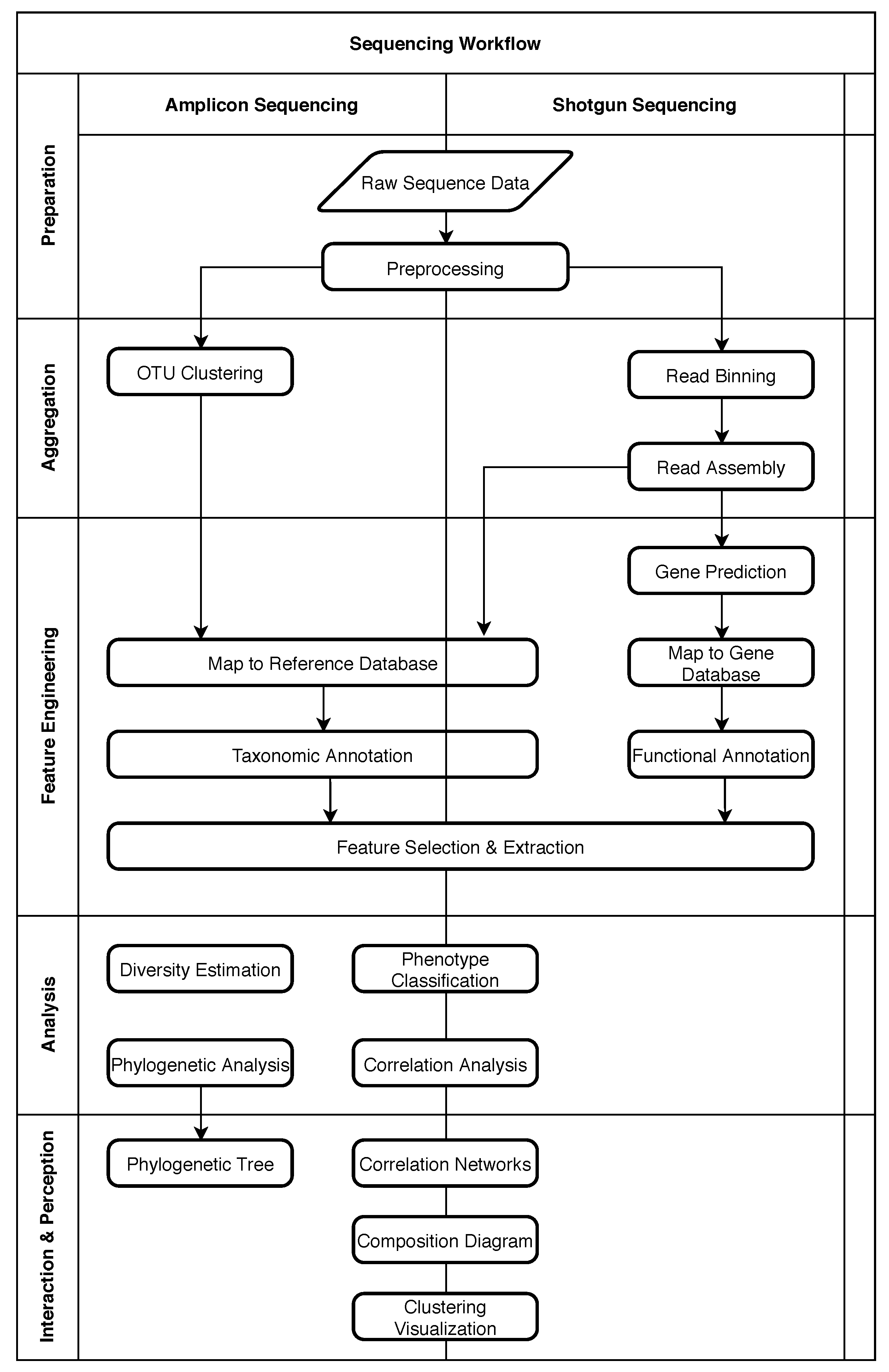
2.1. Five Phases of Metagenomic Studies

The “Preparation” phase encompasses preprocessing of the raw sequence data to make it available to subsequent processes. In metagenomic processing solutions (see Section 6), this can include all necessary steps for data ingestion and format conversion. It also includes steps to ensure the necessary quality of data by trimming or removing low-quality sequences [20].
In the “Aggregation” phase, the sequences are sorted, grouped, and assembled as necessary. For amplicon sequencing, this usually includes a clustering step to identify clusters of closely related microorganisms or Operational Taxonomic Units (OTUs) [25]. In shotgun sequencing, it is often desired to reassemble whole genomes or larger sequences from the short reads produced by the sequencing platform. “Read Binning” can support this process by identifying reads that have a high probability of originating from the same or at least a closely related microorganism so that the “Read Assembly” can be performed more rapidly and precisely [26]. For the assembly, overlaps between sequencing reads are identified and used as an indicator to determine the relative order of fragments. A set of overlapping sequencing reads is called a “contig” [20].
The “Feature Engineering” phase was previously split into two distinct phases called “Annotation” and “Summarization” in the original paper [24]. As “Feature Engineering” is a more established and broader term, and better describes the intent of creating features for the analysis phase, we decided to merge these two phases. During this phase, databases can be used to map sequences to known reference data [26]. In the case of amplicon sequencing, they contain common amplicons and their taxonomic interpretation (e.g., name of the species). Shotgun sequencing, on the other hand, is more often used for “Functional Annotation”, where the focus is no longer on organisms as a whole, but rather on individual genes, which might or might not be shared between organisms. Common databases for gene sequences can include much metadata that can reveal specific functions of a gene within an organism or within an environment as a whole, which can then be used for further analysis. As a general optimization, or in case it is desired to identify unknown genes, it can be useful to perform “Gene Prediction” on sequences beforehand. This process attempts to identify patterns that indicate coding regions within the sequence.
In general, the feature engineering phase is a transitional phase where the focus shifts from gathering data to the analysis and interpretation of said data [24]. This includes all transformational tasks such as the computation of relative abundances, where the previously identified genes or taxa are counted and put into relation to other genes or taxa in the same sample, or other more complex transformations known as “Feature Selection” [27] and “Feature Extraction”, that simplify and reduce the amount of input data for the analysis phase while preserving important information.
As the name implies, the “Analysis” phase contains analytical processes that try to derive new information from the input features. Often it will be the most important step in metagenomic studies, directly supporting the study goals. Therefore, the processing steps are quite heterogeneous, depending heavily on the goal of the study. That being said, frequently used steps include the classification of phenotypes or computing correlations between genes or taxa. Finally, during “Interaction & Perception”, results from analysis or previous steps are presented to the user in a suitable fashion such as interactive visualizations or dialog systems. As with the analysis phase, visualizations are also heavily dependent on the study goals. Note that “Interaction & Perception” was originally named “Visualization” in [24] but was changed to match the AI2VIS4BigData reference model established by Reis et al. [28] and to better describe the possible interactive nature of result presentation.

2.2. Example: Microbiome Analysis on Four Human Body Sites

Wassan et al. [29] considered various data sets containing identified OTUs from 16S rRNA amplicon data on various human body sites. They then demonstrated how metagenomic ML models can benefit from using hierarchical, phylogenetic information (e.g., considering evolutionary distances between OTUs). This section provides an overview of the study and shows how it can be aligned with the five phases mentioned earlier. For the purpose of brevity, only the Human Microbiome Project dataset [30] is used in this description (Figure 2).
The tasks matching the “Preparation”, “Aggregation”, and part of the “Feature Engineering” are described in the supplementary documents of The Human Microbiome Project Consortium [30]. For “Preparation”, QIIME [31] and custom scripts are used to discard low-quality sequences and to de-multiplex sequence data from different samples. To cluster sequences and to pick representative OTUs, UCLUST [32] is used (“Aggregation” phase). Then, the RDP classifier [33] is used in the “Feature Engineering” phase to assign a taxonomy and an OTU table is created while applying additional quality controls.
Wassan et al. [29] continued the “Feature Engineering” phase by creating a phylogenetic tree from the OTU table and then using this tree to conduct feature selection using various algorithms, such as random forest (Section 3.4). Figure 2 outlines this idea. For the “Analysis” phase, Support Vector Machines (SVMs) (Section 3.2), naïve Bayes (Section 3.5), and logistic regression (Section 3.6) were compared for classifying phenotypes given in the original dataset.
The analysis phase forms a promising direction of metagenomic research by uncovering knowledge from the information of compositional profiles obtained from the steps of aggregation and feature selection.
An additional key focus of studies by Wassan et al. is integrating biological domain knowledge of phylogeny [34] with abundance profiles of OTUs, aiding in inferring metagenomic functions from the microbial profiles. Research by Wassan et al. [29] suggests that the use of computation techniques using ML over integrative profiles could improve our understanding of microbial profiles and their functions.
The random forest classification method has typically been employed in the prediction of high-dimensional metagenomic data [35,36] assuming independence between features. By integrating biological knowledge of phylogeny with the quantitative profiles, the prediction of metagenomic functions built upon considering these relationships could better inform metagenomic studies. Wassan et al. [29] employed the incorporation of both quantitative (abundances) and qualitative (biological domain knowledge of phylogenetic relationships) aspects into the construction of new feature space for the prediction of metagenomic phenotypes. A novel framework was proposed to determine metagenomic functions involving (i) engineering of new feature space via integration of biological and quantitative profiles, (ii) application of feature selection strategies over the engineered space, and (iii) application of the classical predictive models (such as random forest, SVM, naïve Bayes, and logistic regression) over the selected features. By employing the integrative approach, an improvement in predictive performance was observed by Wassan et al. [29], in comparison to previously employed approaches [35,36]. Furthermore, features space modeling has been characterized by different levels of varying phylogenetic depth (phylum to genus) in the study by Wassan et al. [29] which seems to be advantageous over traditional work where only features at genus level were considered [35,36]. The studies by Wassan et al. [29] improved modeling over the high-dimensional and integrative microbial feature space for determining functional predictions by involving phylogenetic analysis. Proposed approaches demonstrated high prediction accuracy.
The phylogenetic similarity between microbial genes may also play an important role in determining metagenomic functions. Applying the ordination of Principle Coordinate Analysis (PCoA) over phylogeny and/or abundance wise similar matrix could provide some more support for differentiating microbial samples based on the functional phenotype [37]. As this paper focuses on demonstrating classification improvements for ML algorithms, the visualizations included herein consist of tables showing Accuracy and Kappa values for the different configurations. These visualizations can be generated by using validation metadata obtained during the analysis phase. The same data could also be used in graphical representations.

3. Machine Learning

The two primary uses of ML within metagenomics are classification and clustering. Classification algorithms learn to classify data points into a predetermined set of categories or “labels” from a set of training samples (supervised learning). Clustering algorithms on the other hand try to find and group similar data points without using predetermined classes (unsupervised learning).
Another unsupervised type of ML often used in metagenomics that can be distinguished from classification and clustering is dimensionality reduction [13]. The goal of dimensionality reduction is to decrease the sparsity and complexity of data while preserving key information. These algorithms can be used as a preparational step for other algorithms that do not work well with highly-dimensional data or in the creation of visualizations that are by nature limited to few dimensions.

3.1. Vector Space Transformations

Most ML techniques require their input to be vectors with n dimensions [38], where each dimension corresponds to a feature in the input data that can be used to distinguish the data. A dimension could be something as detailed as the nucleotide present at a specific position within a sample or something more general as the fraction of guanine and cytosine present in the sample (GC content). As the vector components must be numeric, suitable transformations must be applied if the original input data does not fit this criterion [38].
Encoding methods can be distinguished into sparse encoding methods, where most vector components are zero, and dense encoding where the same information is encoded using fewer dimensions and most components are non-zero [39]. For example, the nucleotide at a specific position could be encoded in four dimensions using 0 and 1 to determine the presence or absence of a base or in a single dimension if each possible base is assigned a unique number (e.g., A = 0.25 , C = 0.5 , G = 0.75 , T = 1 ).
Some (simple) ML techniques perform better on sparse vectors, while more powerful techniques tend to perform better on dense vectors.

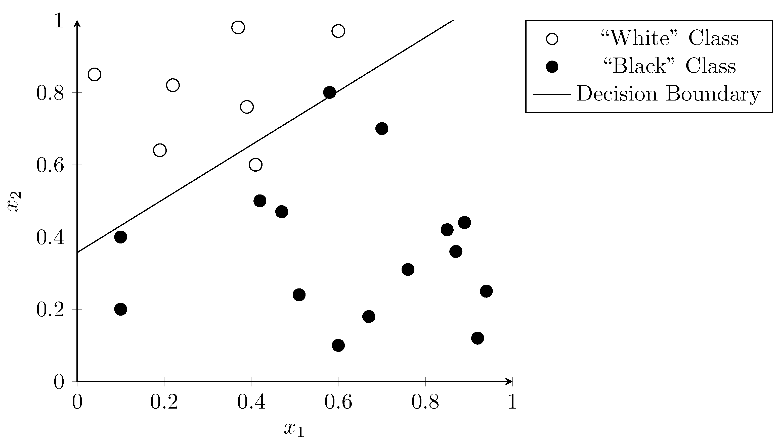
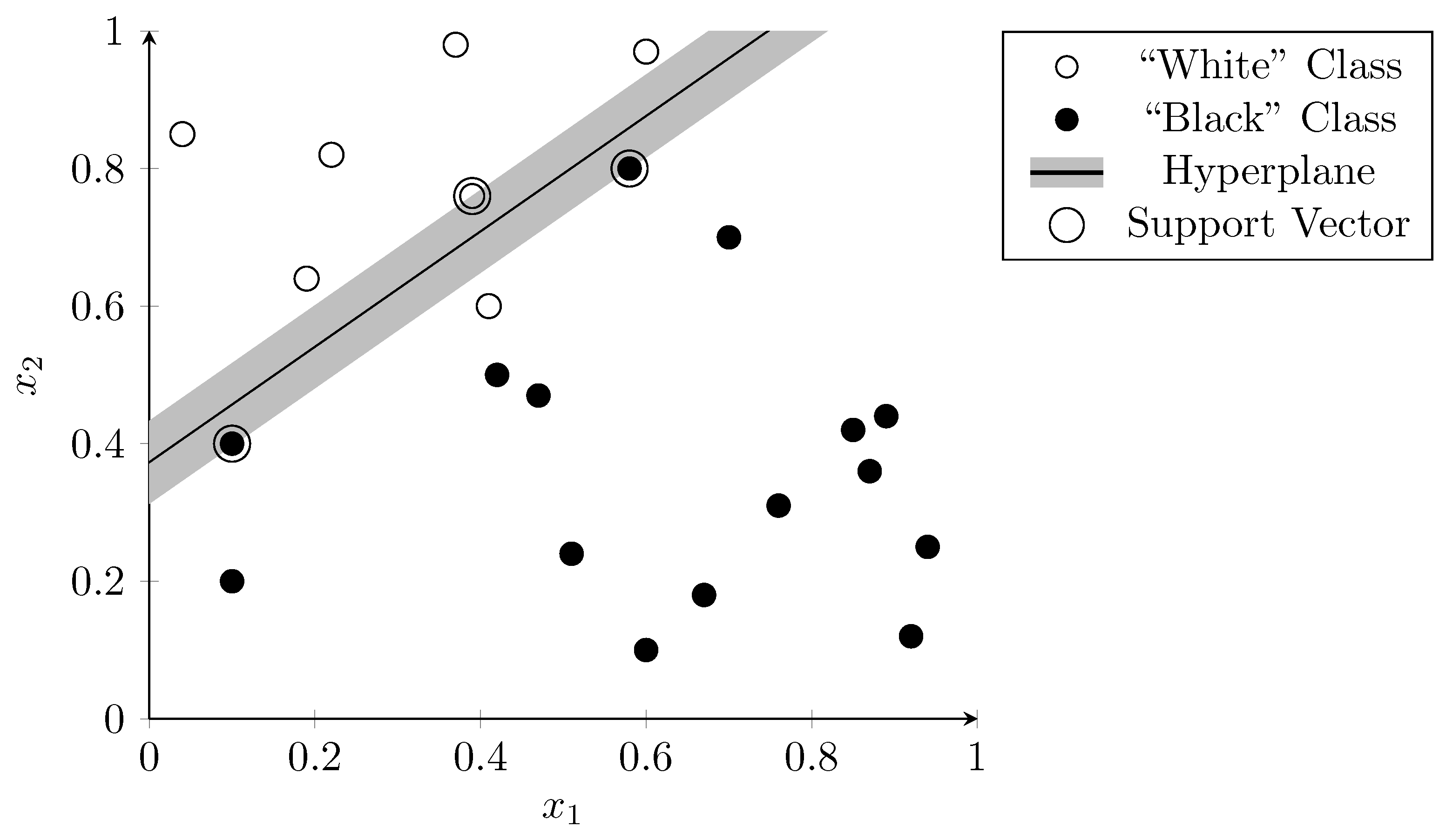
3.2. Support Vector Machines
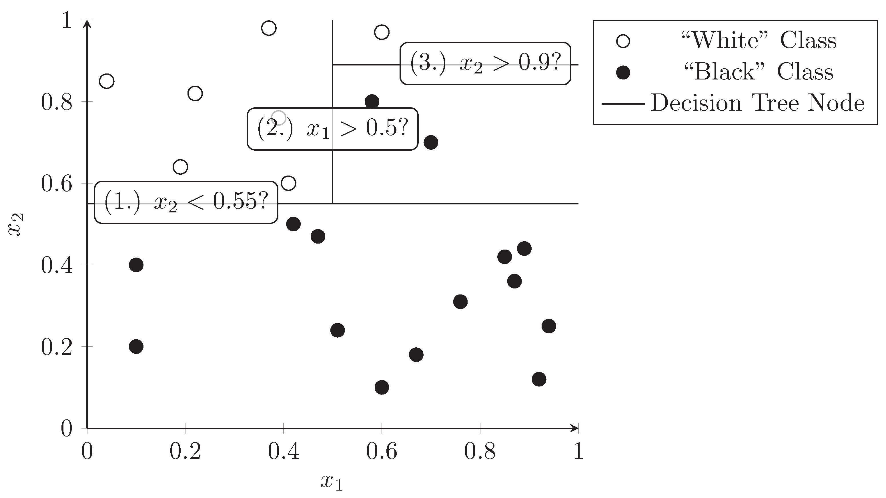
Support Vector Machines (SVMs) [40] are used to separate input data into exactly two distinct classes. This works by computing a hyperplane in the vector space with the largest possible margin between data points of the two classes. A hyperplane is defined as a subspace with one dimension less than the vector space it is contained in. Therefore, in a 2D space, the hyperplane would be a simple line, while in a 3D space it would be a plane and so on.
If such a hyperplane exists the data is called linearly separable. Training an SVM on representative, linearly separable data would result in a perfect classifier with 100% accuracy. Unfortunately, most real-world data is not completely linearly separable due to outliers or complex dependencies between the dimensions that cannot be expressed in a linear way. Thus, most SVM implementations, allow for such errors and try to minimize the error introduced by the outliers while at the same time maximizing the margin between the data points that are linearly separable.
Sparse vector representations improve linear separability as there are more dimensions than the hyperplane can “use” to separate the data. Figure 3 visualizes this using a two-dimensional vector space. The features x 1 and x 2 are arbitrary examples of features that could occur during a metagenomic analysis. The dots represent samples that were used to train the SVM. The correct classification is indicated by the color of the dots—white dots belong to one class and black dots to another. The hyperplane (in this two-dimensional case a simple line), separates the two classes almost perfectly with only one outlier (the white dot below the line). The dots on the edge of the margin (i.e., the vectors that define the margin) on both sides of the hyperplane are called “support vectors” (circled in Figure 3).
Another way to improve linear separability is to project the input vectors into a higher-dimensional space using a kernel function [40]. This is known as the “kernel trick”.
SVMs are a popular choice as they are efficient to train and provide favorable results on many data sets [41]. Their performance drops if the data has complex dependencies and cannot be made linearly separable. Another disadvantage of using SVMs is that they require careful selection of features used as input vectors, as having many dimensions that do not contribute to the classification decision can reduce performance [41].

3.3. Decision Trees

A decision tree is a tree structure where each node splits a data set into two subsets based on a predicate (e.g., x 1 dimension has a value of 0.5 or less). This process can be repeated at subnodes which divide the dataset further into smaller and smaller subsets. A decision tree can be used as a classifier by assigning class labels to the leaf nodes of the tree. The nodes should be constructed in a way that maximizes the predictive value at each level of the tree, i.e., the dimensions and values should be chosen in a way that best separates the data points into the target classes. Figure 4 demonstrates how a decision tree splits the dataset used in the previous section into distinct subsets that only contain one class of points (black dots or white dots). The lines represent a node in the decision tree and the predicate is written in the label. Each side of the line is a sub-branch of this node and can contain further decision nodes.
Using a decision tree alone as a classifier is one of the fastest ways to build a classifier as the tree can be constructed very efficiently [38]. By using a simple binary decision at each level of the tree, the classification decisions are also easily comprehensible by humans which improves the overall explainability of the model (see also Section 5.4).
Unfortunately, decision trees are too simple for many real-world problems and are prone to overfitting, meaning the tree can classify the training data perfectly, but fails to classify new data accurately [42].

3.4. Random Forest

The random forest ML method [43] tries to tackle the shortcomings of the decision tree classifier. It uses not one but several (often hundreds or thousands) decision trees and then bases the final classification decision on a majority vote. As constructing multiple decision trees from the same dataset using the same dimensions would result in the same or very similar trees without improving the classification performance, a special construction logic must be used for the trees. This construction logic consists in using only a subset of the total data for each tree and limiting the dimensions from which predicates can be chosen to a random subset of the total dimensions in each level of the constructed trees. It can be proven that constructing the trees in this way avoids the risk of overfitting even if a large number of trees is used [43].

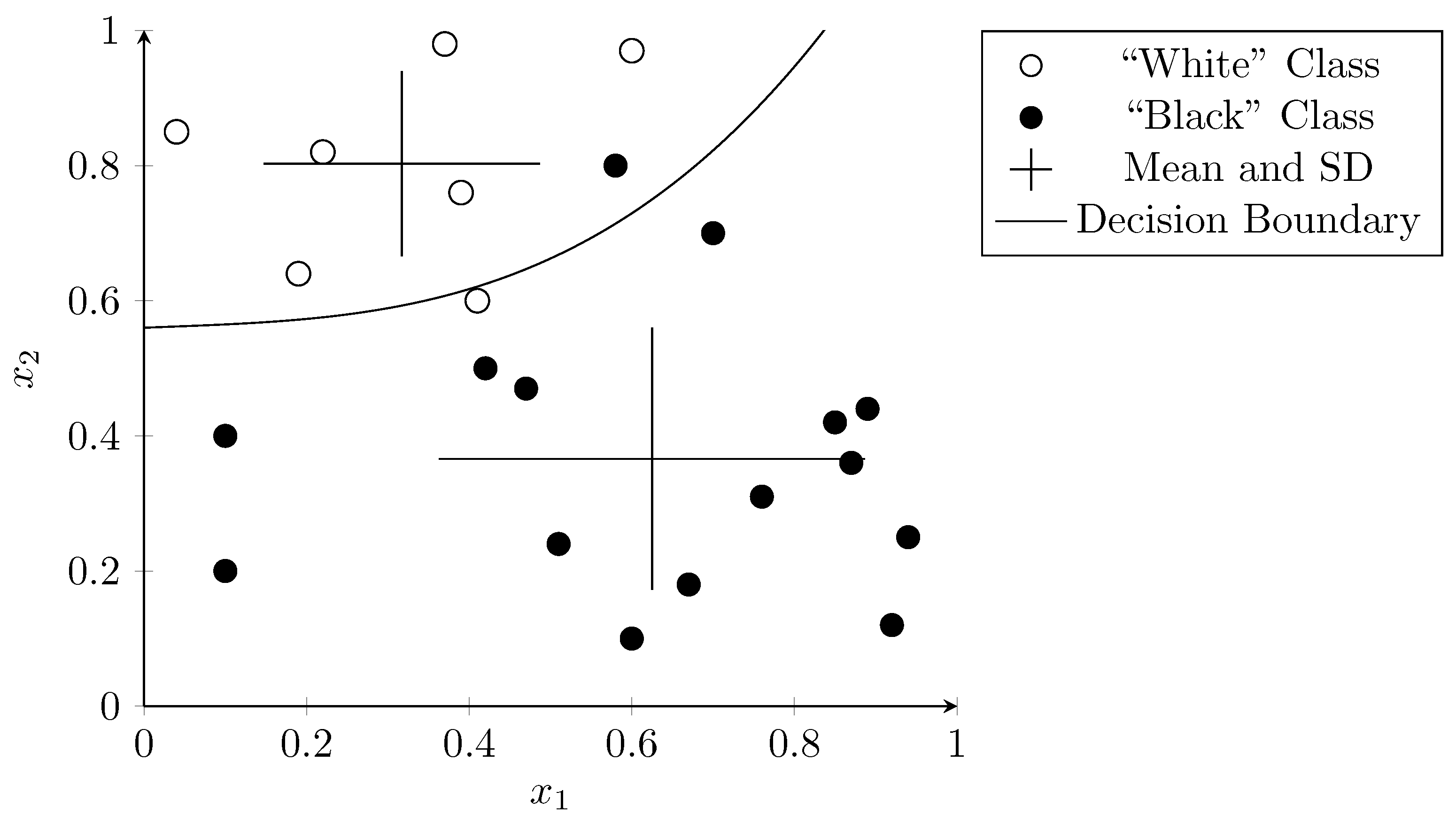
3.5. Naïve Bayes Classifier

Naïve Bayes classifiers are simple models that assume that all dimensions of the input data are completely independent of each other [38], meaning they contribute on their own to the probability of a data point belonging to a specific class or not without taking into account the values of other dimensions. Even if this assumption is often not true, naïve Bayes classifiers can still perform quite well in many cases. Depending on the distribution and type of values (e.g., categorical or continuous), various subtypes exist. For example, the Gaussian naïve Bayes classifier assumes a normal distribution for continuous values, while a multinomial naïve Bayes classifier can deal with categorical values.
Figure 5 shows an example where the normal distribution for black and white dots was computed and shown as crosses originating at the mean and extending to one standard deviation (SD) in each dimension. The probability that a data point belongs to a class depends on this probability distribution. The curve shows the decision boundary where the probability for both classes is the same. Even though there are two outliers, the overall separation works well and categorizes almost all points correctly. Naïve Bayes is popular because of its simplicity and its capability to perform well with very few training samples.

3.6. Logistic Regression

Logistic regression [44] is another simple model that can be used for classification. The model computes a weighted sum of its input vector and then applies the sigmoid function, which is also known as the “logistic function”, to this sum [44]. The result of the sigmoid function can be interpreted as the probability that a data point belongs to a given class. The training of a logistic regression classifier consists in adjusting the weights for the input vector so that the output function best matches the training data set.
As the only input to the logistic function in the classifier is a linear combination of the input values (“weighted sum”), the classifier requires the input data to be mostly linearly separable to perform well (see Section 3.2). Figure 6 shows the result of applying logistic regression to our example dataset. The line represents the decision boundary where the sigmoid function has the value 0.5 , indicating a 50% probability for both classes.
The computations performed in a logistic regression classifier are the same as those in a single neuron of a neural network (see Section 3.8) that uses the sigmoid function as the activation function.

3.7. Clustering Algorithms

As the clustering algorithms used in metagenomics are generally simpler and less diverse than the classification algorithms, they will be described only briefly in this section. In general clustering algorithms try to create clusters by finding similarity between input data and grouping it in a way that maximizes the similarity within a cluster while simultaneously minimizing the similarity between clusters. Similarity, in this case, has to be defined in some way using a distance metric. For metagenomic sequences this could be character-based, i.e., checking what percentage of characters between two sequences is the same, or based on more general properties (e.g., GC-content).
Finding optimum solutions to these problems is generally not possible—even with small datasets—as it requires trying prohibitively many combinations. Therefore, heuristic algorithms are used that aim for a satisfactory balance between runtime and quality. One of the popular algorithms is Lloyd’s algorithm [38], which is often referred to as “k-Means clustering”. In Lloyd’s algorithm, a list of data points is chosen randomly to act as starting cluster centers (centroids). All data points are then assigned to the cluster with the nearest centroid. Afterward, new cluster centroids are chosen by calculating the mean of all data points within each cluster. This last step could change the nearest cluster centroid for some of the data points, thus assignment to clusters and calculating new centroids are repeated until there are no more re-assignments.
While popular due to its simplicity, Lloyd’s algorithm has several problems, which are also relevant in metagenomics. First, the number of clusters must be chosen beforehand, which can be difficult as the best number of clusters is often not known. However, this is solvable by using variants where the number of clusters is chosen dynamically. Another problem is that calculations of mean and distance are based on Euclidean distance and hence require input data to be presented in a vector space (see Section 3.1). While this is also true for most classification algorithms described in this section, clustering algorithms in metagenomics are often used early within metagenomic workflows (see Section 4.3) where other forms of distance metrics (e.g., based on character data) are easier to compute. Finally, Lloyd’s algorithm has a worst-case superpolynomial complexity [45]. Processing huge data sets, as sometimes required in metagenomics, is therefore not always feasible.
While Lloyd’s algorithm has several problems that limit its use in metagenomics, its simplicity and general principles are a sound basis for understanding clustering algorithms in general. Some specific uses will be discussed in Section 4.3 and Section 4.4.

3.8. Neural Networks

Neural networks are inspired by biological neurons. Common to both biological and artificial neurons is the idea that they are interconnected and that each neuron only performs simple computations while the combined network can perform complex tasks such as classification based on many input variables and complex dependencies [46].
The neurons in most models take several real numbered inputs, compute a weighted sum, and then output a value based on a threshold. If the weighted sum is below this threshold the output strives towards one value (e.g., 0 or 1 depending on the model) and if the sum is above the threshold the output strives towards another value (e.g., 1 or the sum itself depending on the model).
Artificial neural networks are usually organized in layers where the output of the neurons in one layer is the input of the next layer [47,48]. The input of the first layer is the features obtained from the samples and the last layer outputs the desired result, e.g., one output for each possible category in a classification task. Intermediate layers serve to enhance the computational strength of the network by allowing the network to “recognize” more complex dependencies within the input data that are required to determine the result [46].
Compared to, e.g., SVMs, neural networks depend less on the data being linearly separable as they are inherently more powerful. An SVM can be mathematically expressed as a single neuron (single layer network), but in contrast, the computations performed in multi-layer networks are generally not expressible in an SVM [49]. This increased power also allows the use of dense encoding techniques as discussed in Section 3.1 and empirical data shows that deep neural networks (see Section 3.9) benefit from this approach [39,50].
On the downside, the complexity of neural networks also demands more computational power to find the optimum values for all weights in the network. Furthermore, the number of variables in the model increases the risk of overfitting [51]. Overfitting occurs when a classifier tries to optimize its parameters to correctly classify all training samples as perfectly as possible at the expense of generalization.
Figure 7 shows the same data points as were used in the previous examples. Here, the dots were used to train a hypothetical neural network. The gray background shows which area is classified as the “black dot” category, whereas the white background shows which are classified as the “white dot” category. The neural network was able to classify all points in the training set correctly. However, it seems unlikely that these irregular areas represent an underlying truth in the data. If the network is overfitted to the data used during training it is likely to misclassify new data points given to it. Intuitively the SVM did a better job at generalization in this example.
Both this risk of overfitting and the required computational power limited the application of larger neural networks for some time. A collection of new techniques together with increased computational power using GPGPUs led to new popularity for neural networks under the label, “deep learning”.

3.9. Deep Learning

Deep learning summarizes a collection of techniques and advancements in recent years [14]. While some of these techniques can be applied to other ML methods, they are most often used in the context of neural networks. The term “deep” in deep learning refers to the higher number of layers compared to classical neural networks, which can improve the predictive power of these networks significantly [14]. In classical neural networks several factors limited the use of many layers:
  • Increasing the number of neurons leads to a higher number of variables which increases the risk of overfitting [51].
  • The processing power for training large networks was not available [15].
  • The popular “activation functions” used in neurons to compute the final output value of the neuron based on its inputs were proven to perform poorly in the context of many layers (known as the vanishing and exploding gradient problems in the literature) [52].
With deep learning these challenges are addressed as follows:
  • Deep learning networks are often trained with a significantly larger quantity of data. Many breakthroughs come from big tech companies like Google that have access to huge datasets (e.g., billions of images) which decreases the risk that the network only memorizes its training input and fails to generalize. Some computational techniques were also developed which keep the network from overfitting (e.g., “Dropout”, see Srivastava et al. [51]).
  • The processing power was increased by offloading the training to the Graphics Processing Unit (GPU) and utilizing large computing clusters. The advent of cloud computing enabled this possibility not only for big companies but also for smaller research teams.
  • The problem of vanishing or exploding gradients was mitigated by using vastly simpler activation functions, which do not exhibit this problem.
Due to these improvements over classical neural networks, deep learning has been able to solve problems that have previously been impossible. It broke records in many disciplines such as speech or image recognition [14] and many products such as digital assistants or search engines now use deep learning.

4. Role of Machine Learning in Metagenomics

In metagenomic studies, there are several steps that use ML algorithms or could potentially use them in the future. This section will cover typical processing steps and identify ML applications. Unless otherwise mentioned, the process will focus on sequencing results from high-throughput platforms like Illumina.
The section is structured along the phases and steps shown in Figure 1. Readers are invited to use the figure as a reference while reading this section.

4.1. Obtaining Raw Sequence Data

The sequencing of DNA fragments works by reconstructing one of the two DNA strands base by base using specially modified fluorescent nucleotides with different dyes [22]. The original bases can then be detected by taking a photo at each step of the reaction and finding the dominating color. Determining the correct base from the images is a process called base-calling. Base-calling is complicated by multiple sources of errors during this reconstruction.
Machine learning has been applied to this problem. One example is the use of SVMs, which showed promising results in a comparison of various base-calling algorithms [53]. However, the literature on base calling using more modern deep learning techniques is sparse. One explanation for this may be that the results of simple algorithms already have low error rates and that there is therefore little room for improvement. In nanopore sequencing (an alternative, emerging sequencing method), where the error rate for base calling is significantly higher, deep learning has been applied successfully, which further supports this assumption [54,55].
After base calling the (digital) result of the sequencing operation will be a collection of “reads” representing the fragments that were sequenced with corresponding bases and quality metrics [20].

4.2. Preprocessing

Common preprocessing steps to be applied on raw sequencing data include demultiplexing reads from various samples by identifying attached barcode sequences, discarding or trimming low-quality reads, and removing sequencing artifacts.
A review of relevant literature revealed no significant use of ML in these areas. State-of-the-art toolsets like QIIME 2 [31] use relatively simple rules for these steps.
Some authors [19], however, do see potential for deep learning models that cover the entire processing pipeline, including preprocessing steps, in the future.

4.3. OTU Clustering

For amplicon sequencing a common next step is to cluster reads belonging to the same species or higher taxonomic rank into OTUs for later processing by searching for reads with similar sequences (typically, 97%) [25]).
The goal of clustering into OTUs is to reduce the quantity of data that needs to be processed in later steps. Clustering was discussed in Section 3 as one of the two important branches of ML types. Accordingly, there are several algorithms that can be used in this task [13].
One popular algorithm is UPARSE-OTU [56]. UPARSE-OTU is a greedy algorithm (Section 3.7) and thus assigns clusters in a single iteration. The algorithm starts by ordering input sequences by abundance as a high abundance indicates a non-erroneous read and therefore might be good OTU candidates. Starting from the first sequence, the algorithm will either assign the sequence to an existing cluster, create a new cluster using the sequence as the OTU reference sequence, or discard the sequence if it is believed to be chimeric. A sequence is assigned to an existing OTU cluster if its similarity is above 97%. Similarity is defined here by the UPARSE-REF algorithm [56] which uses a maximum parsimony model, i.e., defining similarity by the number of “events” that need to occur to go from one sequence to another sequence (e.g., a sequencing error). As the Maximum Parsimony model is a satisfactory approximation of similarity, there is little practical usage of more advanced ML models.

4.4. Read Binning

Another use of clustering algorithms is for the purpose of “Read Binning” in shotgun sequencing—often used as an optimization step before sequence reassembly. Binning tries to separate reads from different organisms so that the reassembly process is easier and less prone to false overlaps between only far-related organisms [26].
In contrast to OTU clustering, where sequence reads are expected to map to the same position/amplicon, the actual overlap between two sequences belonging to the same “bin” can be less or non-existent as the individual reads map to a longer sequence. Instead of relying on sequence similarity, binning algorithms hence often rely on other similarity measures such as k-mer distribution or probabilistic models [13]. The former relies on the fact that the distribution of k-mers (i.e., short subsequences) is similar within a genome while the latter attempts to model probabilities for reads to belong to the same bin and then uses expectation maximization to find the most likely result. Early attempts also used neural networks for this task [57].

4.5. Read Assembly

HTS platforms are limited to DNA fragments with a few hundred bases at best for technical reasons [22]. This can be sufficient for many metagenomic applications. For example, phylogenetic studies based on amplicon sequencing can use rRNA regions that are short enough to be read completely but still unique enough to differentiate species [23].
When complete genomes or larger sequences need to be sequenced, they need to be split up into fragments smaller than the maximum read length of the sequencer first [22]. However, this creates two problems: First, the order in which the fragments originally occurred within the genome is lost, and second, the organism from which the fragment originated is also unclear as the fragment gets mixed with fragments of all other organisms in the sample [9]. This is not necessarily a problem if only the presence and abundance of certain genes in the sample need to be known. In this case, it can be sufficient to match the fragments directly to adequate databases for the research topic [26]. However, in other cases, the reassembly of the original genomes present in the sample is desired.
Reassembly happens by finding overlaps between the reads and aligning them on each other. Several strategies and tools exist for this [20] and some of them are specialized for metagenomics [26]. There are some promising results for genome reassembly using both classical ML algorithms as well as deep learning techniques, but most of them are still relatively new and their performance on real-world samples is yet to be determined [58].

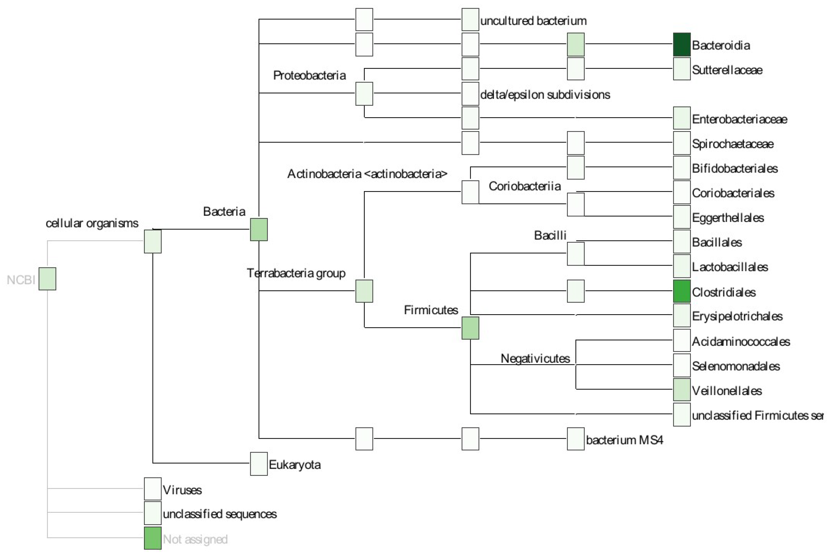
4.6. Taxonomic Annotation

Taxonomic assignment is the task of choosing a label for each sequence or cluster based on a chosen taxonomy, e.g., finding the species that a sequence is associated with. To facilitate this, reference databases with sample sequences for the various labels can be used. The methods for taxonomic annotation can broadly be separated into two groups. The first group of methods is used in amplicon sequencing and utilizes rRNA databases. Here, one of the most popular tools is RDP classifier [33], an ML approach using a naïve Bayes classifier. The second group constitutes methods for assignment of reads or clusters of reads taken from shotgun sequencing in whole-genome studies. In this group, non-machine learning-based approaches like Kraken [59] which rely on exact substring matches seem to be more popular.
One challenge faced by ML algorithms is the large number of possible species and similarities between substrings in even distant species [60]. However, there are some indications that less reliance on exact matches could also be a strength for ML algorithms when dealing with species not part of the training set [13,60]. This is particularly important when comprehensive reference databases for the chosen environment do not exist. For many microbiome environments, whole-genome samples only exist for common or otherwise interesting species [26].

4.7. Functional Annotation

While taxonomic annotation tries to answer the question of “what is a sample composed of?”, functional annotation tries to answer the question of “what do the components do?”. Initially, the task can be very similar to that of taxonomic annotation. However, the reference databases used in functional annotation consist of individual genes and associated functional categories. In this case, the challenges for ML algorithms are very similar to taxonomic annotation, and ML is hence not often used for this task [13].

4.8. Gene Prediction

However, machine learning is often used in gene prediction [13]. Gene prediction tries to find genes within samples without matching them to existing databases and is thus often one of the first steps when exploring new genomes. A challenge in metagenomics is that complete genomes can often not be assembled so that the analysis can only be based on individual reads or partial assemblies. Most gene prediction algorithms are based on hidden Markov models [13]. Other popular tools for metagenomic gene prediction use neural networks [61] and there have also been successful attempts to apply deep learning to the task [18,62].

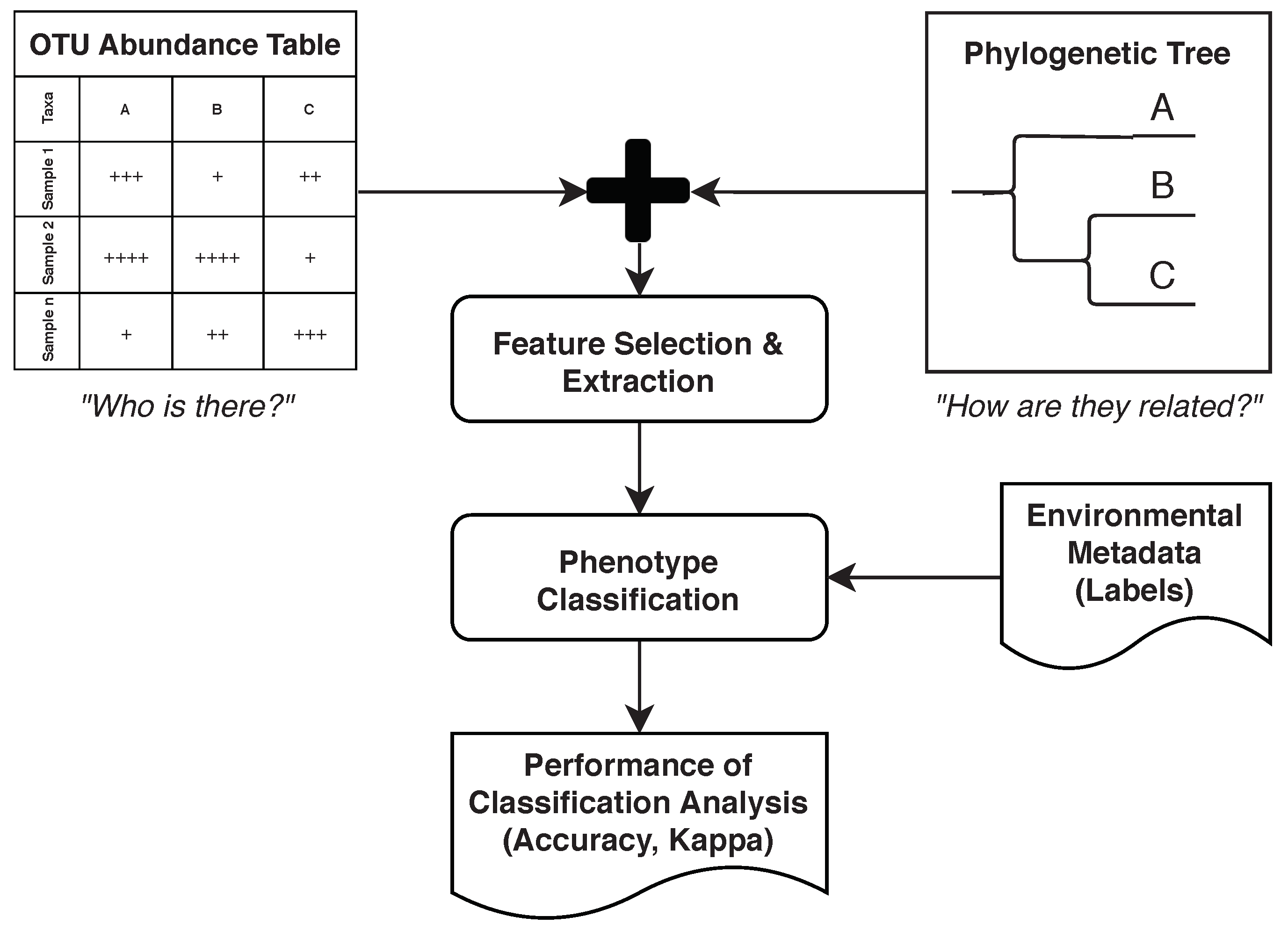
4.9. Feature Selection and Extraction

“Feature Selection and Extraction” is usually applied for removing irrelevant and redundant features from the high-dimensional metagenomic datasets. Three standard techniques are [27] (i) filter-based techniques that use heuristic functions over general statistical characteristics of data to determine important features such as correlation between features, (ii) wrapper-based approaches that iterate an ML algorithm over the input features to determine important features, and (iii) embedded methods intended to determine features by measuring performance while the model is being constructed.
Wassan et al. [63] conducted a comprehensive analysis of metagenomic data from human microbiomes with application of different feature selection strategies. They recommended the application of embedded feature selection methods, namely, extreme gradient boosting (XgBoost) [64] and penalized logistic regression to determine important microbial genes in metagenomic studies. Automatic selection and weighting of features is one of the promises of deep learning, which could make this separate step obsolete in the future [14,15].

4.10. Phenotype Classification

In phenotype classification, one trains a classifier to predict certain characteristics based on metagenomic sample data. Starting from training data where both the metagenomic sequences and the associated phenotype are known, the classifier learns to apply the categories to previously unseen data. This helps us to answer questions like “How can sick and healthy individuals be distinguished by their blood microbiome” [65], “How does the maternal microbiome affect the development of newborns?” [1], “What role do microbiomes play in the relationship between diet and metabolism?” [2], “How do microbiomes interact with the immune system?” [3,4], and “How do they relate to diseases?” [5,6]. These classifications can be based on relative abundances of taxa or genes, and additional features obtained from the samples [13,63].
All of the supervised learning algorithms discussed in Section 3 can be used for this task. The example introduced in Section 2.2 used, for example, SVMs (Section 3.2), naïve Bayes (Section 3.5), and logistic regression (Section 3.6). While still rare, some studies also use deep learning for phenotype classifications [17], although successful application is often a challenge due to an insufficient number of samples [19] (see also Section 5.7).
Nevertheless, recent advances open up a new avenue for applying deep learning models in data analysis [66]. For example, Zhu et al. [67] successfully applied a new deep learning model called Deep Forest [68] to investigate microbiome associations. One key advantage exhibited by Deep Forest is that it can work well even with small-scale training data.

4.11. Other Common Analysis Tasks

Other frequent analysis tasks include, for example, diversity estimation, phylogenetic analysis, or correlation analysis. Diversity estimations are statistical measures to determine the variety of species present within a sample (alpha diversity) or the different composition between samples (beta diversity) [37]. Correlation analysis measures the relationships between different genes or species across samples. In a positive correlation, the increase of one gene or one species increases the abundance of another gene or species. In a negative correlation, the increase in one leads to a decrease in the other. Both analyses are based on statistical measures and can be computed directly from the compositional data of samples. To our knowledge, there are no attempts to provide alternative measures using ML.
Phylogenetic analysis tries to determine the evolutionary relationships between microorganisms and to order them within a phylogenetic tree. In general, algorithms in this category treat genetic mutations as a distance measure. The closeness on the phylogenetic tree depends on the number of mutations required to explain sequence differences between two species. The algorithms to compute these distances and to construct phylogenetic trees from the set of all sequences range from simple distance methods to more complex probability-based models [69]. Machine learning algorithms are not frequently used.

4.12. Interaction and Perception

Visualizations are an important tool to understand the data generated at various steps. One example is the visualization of sample composition using taxonomic or functional annotation data. Figure 8 shows a sunburst diagram created with the free software Krona [70] and using the dataset from [71]. The rings of the sunburst diagram represent different levels in the phylogenetic tree, with the outer rings being more and more specific. The size of the ring sections is determined by the relative abundance within the sample.
Figure 9 shows another example of taxonomic composition using a phylogram. It was created with the software Megan [72] using a dataset from [73] (sample file AS53_18). In contrast to the sunburst diagram, the hierarchical structure of the phylogenetic tree is emphasized more while the relative abundances are only shown as a heat map and, thus, more difficult to compare. Both visualizations are examples of combining a “Composition Diagram” with a “Phylogenetic Tree”, emphasizing one or the other aspect.
For simple graphics or diagrams, ML algorithms are not needed. However, there are often cases where highly-dimensional data needs to be presented to the user in a way that highlights important features while discarding non-essential data. This is a typical use case for dimensionality reduction algorithms. Examples include the creation of correlation networks or visualizations of clustering and binning (see Section 4.3 and Section 4.4). A practical application for this is described in Laczny et al. [74].

5. Challenges for Machine Learning in Metagenomics

Machine learning can be used successfully in many key areas of metagenomics. However, there are several challenges when applying ML to metagenomics, some of which might also impede broader usage of more advanced techniques like deep learning.

5.1. Model Selection

As seen in Section 3, many ML approaches can be used in the field of metagenomics. Within complex approaches such as neural networks, the models themselves have infinite possible configurations (e.g., number of layers and neurons) to choose from. Finding a satisfactory model is often a difficult and time-consuming task even for experts in the field. It can involve a lot of trial and error without a guarantee that the result will outperform older or simpler models [75]. The necessary time and knowledge to select the best model for a specific task from a myriad of options are often lacking.

5.2. Deep Learning and Feature Engineering

Deep Learning requires new approaches to really gain an advantage compared to simpler ML models. While simple models require careful feature selection and will fail to detect meaningful patterns if the input space is too large and complex, deep learning promises to find suitable representations and meaningful connections in a large feature space without requiring the same level of domain expertise and feature engineering beforehand [14,15]. Just switching out algorithms and using the same features for deep learning neural networks that were used for simple ML models will limit their potential or might even make them perform worse than the simpler models.
On the contrary, the feature space should be extended by adding data from additional data sources where possible to take full advantage of these advanced ML models. Examples in the clinical field include models that not only take into account data from the metagenomic data itself, but also the patient’s medical history or other laboratory data. As with the model selection itself, using deep learning and selecting relevant features is a difficult task requiring suitable architectures and ML expertise, which are not always available. Including additional data sources increases its complexity even further.

5.3. Accessibility

Deeply related to the challenges of selecting a model and features is the accessibility for these processes in analysis systems. Assuming that experts in metagenomics are not usually experts in ML and that hiring ML experts for a metagenomics project is not always an option, the process of selecting models and features should also be accessible for non-data scientists. This is a challenge specifically relevant for the user interface used in these systems, which needs to allow flexible configuration of analysis tasks and model configuration for all kinds of use cases while still being easy to use.

5.4. Explainability

Explainability strives to make the reasoning behind decisions taken by automated algorithms, such as ML methods, more transparent. More explainability is in high demand. For example, the European Commission has committed itself to a more trustworthy and secure use of artificial intelligence (AI), which includes explainable AI [76]. This is particularly important for the field of medicine as decisions can have far-reaching consequences and there is a high demand for understanding what specific reasoning led to them [77].
However, explainability is not straightforward with complex ML algorithms as these are often black boxes. Specifically with deep learning, the large number of layers and neurons can make it impossible to understand the reasoning behind a decision taken by the algorithm. Designing models in a way that improves explainability is possible but could lead to decreased accuracy, although there is some debate about whether this is necessarily true [77]. It is worth questioning the practical importance of explainability [78]. Assuming that there is in fact a trade-off between accuracy and explainability, there are certainly patients and physicians that would prefer a hypothetical black-box algorithm that is 99% accurate in predicting a medical condition instead of another hypothetical algorithm that is only 90% accurate but provides full transparency in its decision process. There are also numerous examples in classical medicine of effective treatments that have been used without knowing why they work [78].
Both determining the need for explainability and managing the possible trade-offs between explainability and accuracy are challenges when implementing new clinical solutions utilizing ML.

5.5. Reproducibility

Closely related to explainability is the concept of reproducibility. In a metagenomic analysis, multiple steps are needed between the initial raw data and the final visualization or result data. It is crucial to be able to reproduce these steps whenever necessary. While this can be done by vigorously documenting each processing step, it is not an easy task as results can depend on the exact parameters of the involved tooling or even a specific environment or version number [79]. It is also easy to make mistakes if these steps have to be performed by hand. The use of ML and trainable classifiers, such as neural networks, can increase this problem as the classification results can change with every retraining of the model, even if the input data remains the same.

5.6. Biological Diversity

The microbiome in human hosts and other environments can contain millions of species and genes [13]. Many of those are still unknown, which can make taxonomic or functional annotation of sequencing data difficult. Existing computational methods and databases also have a bias towards bacterial data, which makes analyzing the whole metagenome including archaea and fungi more difficult [13,80].
Even phylogenetically distant species often share a lot of similarities, which can be a problem with using ML algorithms looking for these patterns. Simple algorithms relying on exact matches are thus often preferred to less strict ML algorithms in taxonomic annotation tasks based on shotgun sequencing (see Section 4.6) [60]. On the other hand, less reliance on exact matches could also be a strength for ML algorithms when dealing with species that are not part of the training set [13,60]. This can be important when comprehensive reference databases for the chosen environment do not exist yet [26].

5.7. High Dimensionality and Low Number of Samples

The nature of metagenomics often leads to relatively few samples (e.g., blood samples from a dozen patients) with very high dimensionality, i.e., thousands or millions of species in the sample [19]. This combination makes it difficult for ML algorithms to find clear patterns in the data that can be used in their decision processes. Modern ML algorithms like deep learning neural networks work by training many parameters and do not need the same level of feature selection as classical algorithms. The ability to infer suitable data representations on its own is one of the greatest strengths and a defining characteristic of deep learning [14,15].
However, this ability usually requires access to large data sets, to allow the algorithm to recognize complex patterns [15,81]. Having access to such datasets with labeled data is, therefore, crucial for metagenomics. Large datasets of, e.g., patient data, can be difficult to obtain, however, as the process of collecting and processing a large number of samples is still expensive, and legal requirements also need to be taken into account.

5.8. Big Data

Big Data is often defined by the three V’s: volume, velocity, and variety [82]. Each of these can be relevant in metagenomics and represent a unique challenge. The volume of data results from the usually large number of sequencing reads required to identify and differentiate the microorganisms found in metagenomic samples. These can lead to many gigabytes or even terabytes for a single study. During processing (e.g., for metagenomic assembly), the required system memory can also reach several terabytes. This is out of reach for desktop computers and requires special infrastructure [13,26]. The secure archival and storage of intermediate and final results presents another challenge as archiving of all intermediate results can increase the amount of storage needed manyfold [79]. Archival must also comply with all legal requirements including minimum and maximum retention times for various types of data in an automated way.
The second “V”, “Velocity”, refers to the speed at which new data is being generated and specifically for metagenomics the rapid growth of data. The total quantity of sequence data has been growing exponentially, doubling approximately every seven months, and is expected to reach the quantity of data produced by other big data applications such as astronomy, YouTube, or Twitter [11]. Metagenomic applications need to be able to scale with this increasing quantity of data, which is a challenge both for algorithms that need to be efficient and for infrastructure, which needs to be scalable [79].
For deep learning the volume and growth of metagenomic data could become a problem for training the algorithms “on-site”. Looking at fields like image or text processing some models are trained using such large quantities of data in order to improve classification performance that the cost of training becomes prohibitive for all but a few very large corporations [83,84]. There is a growing trend of separating training and usage of ML models or to use transfer learning, where existing models are adapted and retrained to specific use cases [85]. Metagenomic systems that integrate ML models should be prepared to allow these hybrid approaches.
Last, the “Variety” of data results from different data formats used and the combination of sequencing data with other data sources for analysis, which can include unstructured or semi-structured data such as scientific publications or medical histories. Integrating all these types of data so that they can be processed together is a challenge [86].
A common approach in big data applications is to split the processing of data into individual steps. These steps can then be optimized separately, e.g., by using parallelization. This separation also facilitates configuration of study-specific workflows in the form of metagenomic pipelines, which is the topic of the Section 6.

6. Metagenomic Processing Pipelines

Many projects aim to facilitate metagenomic or biomedical analyses in general by providing step-by-step processing pipelines. In a pipeline, individual components work together to create a result. The output of one step in the pipeline is the input for one or more following steps. This allows flexible reconfiguration of the pipeline or individual steps depending on the requirements. At the same time, configured pipelines can be saved and reused later for similar studies. Individual steps can easily be replaced with alternative approaches as long as the input and output formats stay the same. This section will provide some examples of these projects.

6.1. Galaxy

The Galaxy project [87] is a web-based platform for biomedical analyses including tools for metagenomic research [88,89]. It integrates several thousand tools in its “ToolShed” ready to be used in custom workflows that can be defined in a visual interface. There are tools to cover the complete metagenomic workflow from the processing of raw sequence data up to visualizations. Galaxy also provides access to a wide range of ML tools and algorithms including popular libraries like scikit-learn [90] and Keras [91]. The project is enabled to support many concurrent users using an infrastructure scalable across multiple computing nodes. It can be used on free public servers, pay-as-you-go cloud services, or installed locally.
Galaxy processing is based on files. Individual processing steps can consume files from previous processing steps and output their results as new files. This facilitates adding existing tools to Galaxy by creating a wrapper that describes its expected inputs and outputs. However, this reliance on files can have disadvantages. First of all, data has to be constantly written into suitable output formats only to be parsed again by the next step in the pipeline, which is inefficient. Furthermore, the execution of new steps cannot start until the files from previous steps have been written completely. Finally, parallelization of individual processing steps is more difficult as the data contained in files cannot be easily split without reading and parsing the whole file.

6.2. MG-RAST and MGnify

MG-RAST [92] is an open submission platform for metagenomic data, that integrates automatic processing like taxonomic and functional annotation of sequence data. Data submission is possible using the web-based interface, a scripting interface, or a REST-based API. As the focus of MG-RAST is on ease of use, fast processing, and using standard procedures across all submissions, the pipeline is fixed and customization is limited to setting several parameters before starting an analysis. As an archive, MG-RAST has an extensive repository of metagenomic data with over 473,000 metagenomes containing more than 2000 billion sequences (as of November 2021, www.mg-rast.org, accessed on 4 November 2021). As MG-Rast does not allow custom pipelines to be used, it is not possible to extend the processing with new machine learning-based steps. There is also little use of ML in the fixed pipeline itself.
A similar solution is offered by the European Bioinformatics Institute (EBI) as MGnify (formerly EBI Metagenomics) [93]. Like MG-Rast the platform allows free submission and analysis of metagenomic data using fixed pipelines. Depending on the type of study performed (e.g., shotgun or amplicon-based analysis) different pipelines are available providing all usual processing steps like functional and taxonomic annotation and a range of visualization and comparison options.

6.3. QIIME 2

In contrast to the other tools in this section, QIIME 2 [31] does not aim to be a full-fledged platform with ready-made workflows accessible through an easy-to-use interface. Rather than that, it is a collection of python scripts that can be used together to do metagenomic analyses locally. Using the command line as the primary interface provides a lot of possibilities for customization and facilitates integrating other command line-based tools into the workflow. Documentation of the steps in a metagenomic study is also straightforward through providing the executed command lines within the paper or in a shell script in an accompanying source repository. The commands are designed to be run locally by default, although it is possible to run some of the jobs in parallel or on a cluster. For developers, the script-based nature of QIIME 2 facilitates integrating ML algorithms as new processing steps. The source code repository includes an example of training a random forest model for phenotype classification [94].
Although QIIME 2 provides a GUI as an API as alternatives mean to access its functionality, the focus is clearly on the script-based interface, which makes it difficult to use the tools as a user not familiar with command-line interfaces and scripting. Setting up clusters to run commands in parallel is also not straightforward and to our knowledge, there is no hosted, web-based interface that allows complete access to the functionality of QIIME 2. QIIME 2 is not a complete workflow system on its own as the user is entirely responsible for the execution of tasks and the management of intermediate and final results. However, QIIME 2 can be integrated into other biomedical workflow systems such as Galaxy.

6.4. MetaPlat and Successors

The idea of MetaPlat is not only to provide comprehensive analysis tools for metagenomic data, but to support the complete life cycle of metagenomic studies, including archiving, taxonomy management, and visualization of results. To achieve this, it is integrated with the Knowledge Management Ecosystem Portal (KM-EP) [12]. The architecture was designed based on best practices of big data systems, to ensure scalability. Another goal was to use new and innovative ML models and visualizations to help researchers in understanding the collected data [95,96].
The system supports reproducibility and tracks the phenotypic information associated with each sequence, including its origin, quality, taxonomical position, and associated biological genome, and produces automated reports and visualizations. Additional objectives of MetaPlat include the following:
  • Sample gut collection, from cattle, for sequencing
  • Collection of publicly available databases to create a new classification of previously unclassified sequences, using ML algorithms
  • Development of accurate classification algorithms
  • Real-time or time-efficient comparison analyses
  • Production of statistical and visual representations, conveying more useful information
  • Platform integration
  • Insights into probiotic supplement usage, methane production and feed conversion efficiency in cattle
The bioinformatic workflow engine used by default in MetaPlat is called Simplicity [97], developed by the company NSilico. MetaPlat is an EU-funded Horizon 2020 project developed by several universities and other organizations, including some of the organizations represented by the authors of this paper. MetaPlat was validated and used for the use case of rumen microbiome analysis.
Partly inspired by MetaPlat, but with an even stronger focus on AI and the goal of expanding its use beyond rumen microbiome analysis, another conceptual architecture was recently presented and initially validated. The “AI2VIS4BigData Conceptual Architecture for Metagenomics supporting Human Medicine” is described in detail in the Section 7.

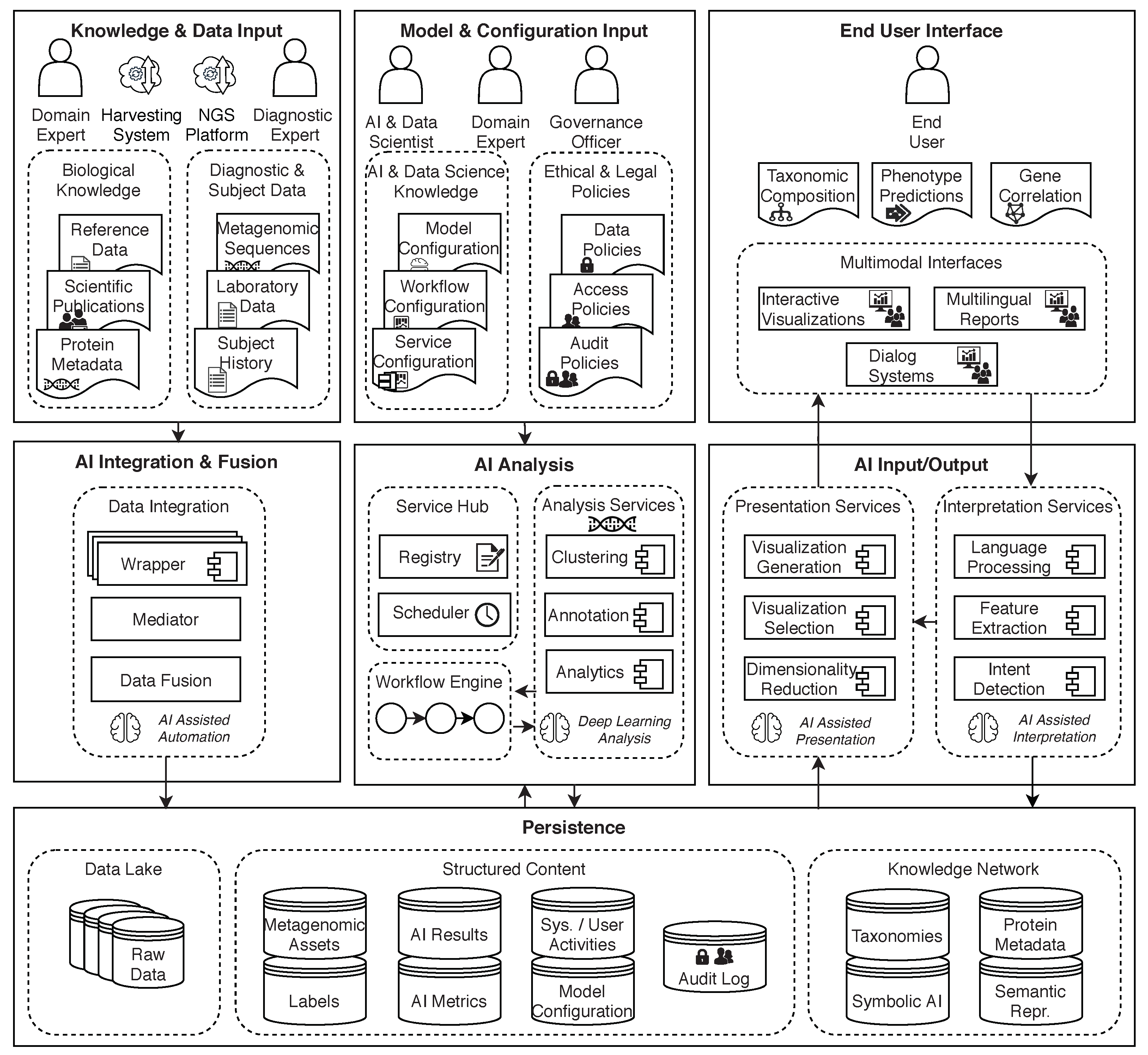
7. AI2VIS4BigData Conceptual Architecture for Metagenomics Supporting Human Medicine

To support the applications discussed in this paper, including addressing some of the challenges described in earlier sections, a conceptual architecture for AI and big data supporting metagenomics research (Figure 10) was introduced in Reis et al. [98]. It is based on the general AI2VIS4BigData reference model [28] for AI and big data applications.

7.1. Description of the Conceptual Architecture

The AI2VIS4BigData architecture is split vertically into three pillars to separate data ingestion from analysis and visualization, applying the design principle of Separation of Concerns (SoC) [99]. Each of these pillars is split into three layers, following the Model View Controller (MVC) [100] pattern, to separate the persistence (Model) from the user interface (View) and the application logic (Controllers). The persistence layer is shared between all three pillars.
The first pillar is responsible for data ingestion. Data such as metagenomic sequences or other laboratory data as well as subject-independent reference data is imported into the system and processed using a mediator/wrapper approach [101]. The wrapper is responsible for transforming the data into a common schema and the mediator is responsible to facilitate communication between the individual data sources and the rest of the system. The intent behind this is that the data formats that can be imported should be easily extensible. Another important aspect of the data ingestion pillar is the storage of raw data in a data lake. This allows better transparency and reproducibility as all steps can be repeated starting from raw data.
In the second pillar, data is taken from the persistence layer and then processed for analysis using a workflow engine to orchestrate the required metagenomic tasks. The configuration for these tasks is provided by domain and data science experts using a configuration user interface. The results are persisted into structured storage again.
Finally, the third pillar is responsible for presenting the persisted analysis results to the end-user and possibly entering into a dialog with the user to further adjust the presentation.

7.2. Use in Clinical Settings

In Section 2.2, an example was introduced in which human metagenomic data is used for the classification of phenotypes. So far, the conceptual architecture presented in this section was only validated for the use case of rumen microbiome analysis. While it seems trivial at first to apply the same architecture for human microbiome analysis in a clinical setting, there are some details to consider that merit another validation by comparing both use cases.
Looking at “Knowledge & Data Input”, there is no fundamental technical difference between the raw sequencing data used in our example compared to the examples in Krause et al. [24] using rumen samples. There might be different supplementary data like medical history or specific databases targeted for human diseases that differentiate these use cases. As the conceptual architecture does not impose limits on the type of data to be used this is not a problem. Likewise, the roles of “Domain Expert” and “Diagnostic Expert” were chosen broadly so that they can be filled by experts in biology, medicine, or others as needed. The “AI Integration & Fusion” layer allows the integration of various data types, bridging their technical differences. This will allow different types of data by implementing suitable wrappers, thus supporting both use cases. The “Persistence” layer does not impose schema restrictions that would either impede clinical use cases.
For the “Model & Configuration Input” layer there may be different legal requirements, like stronger data protection requirements, when comparing both use cases. As the architecture uses a policy model and the role of a “Governance Officer”, these legal requirements can be presented in implementations using the architecture, for example, by using access policies and auditing the use of data. The analysis steps and algorithms, like the use of QIIME 2, UCLUST, and RDP classifier in the human example are similar or identical to the tools used in rumen microbiome analysis. The specific tools used vary from study to study in both use cases, which is addressed in the model by using a configurable workflow engine and a registry allowing for different analysis and processing services to be used.
The “End User Interface” and “AI Input/Output” layers are also very generic to support a wide range of use cases. For rumen microbiome analysis the use of dialog systems or multilingual reports might not be necessary if the role of “End User” is filled by a researcher, who is also a “Domain Expert”. For clinical settings, the “End User” may actually be the patient, who wants an easily understandable report of his diagnosis. As it is, the conceptual architecture does support both use cases.
This initial validation shows that all layers are generic enough to support both use cases. It can thus be assumed that the conceptual architecture as a whole also supports both use cases.

8. Remaining Challenges, Conclusions, and Outlook

The increased use of sequencing technology in the biomedical field and the voluminous quantity of associated data provide several challenges for data processing and opportunities for leveraging advanced ML techniques. This paper provides an extensive overview of both metagenomics and ML in the hope of further bridging the gap between these two disciplines.
With the same goal, several existing use cases for ML in biomedical workflows have been documented. The use case of using phylogenetic information to improve phenotype classification was discussed in detail. Integrating phylogeny directly at the level of the ML model, instead of at data preparation and modeling level, has the potential to provide new microbial features for classifiers such as deep learning neural networks and to improve overall phenotype classification performance.
Possible reasons for the perceived lack of advanced ML techniques like deep learning have been identified, like the lack of sizable training data, accessibility, and general challenges related to big data. Automatization pipelines can help to address some of the challenges associated with big data processing, metagenomics, and ML by improving reproducibility, accessibility, and dividing the work into smaller processable units. With this in mind, they also provide a foundation for the use of advanced, computationally-expensive ML algorithms like deep learning neural networks.
The AI2VIS4BigData Conceptual Architecture for Metagenomics was given as a solution to integrate automated biomedical pipelines while taking into account additional research aspects such as data ingestion, management, archiving, and visualization. It was built with advanced, machine learning-based analysis methods in mind and supports large quantities of data using a distributed and modular architecture. Taken together, these features improve the accessibility of machine learning-based analysis methods and the handling of big data. It was demonstrated that the architecture is suitable for studies in human metagenomics such as the one discussed in this paper, therefore providing an initial validation for the architecture that was previously only validated for use in rumen microbiome analysis.
Future research could address the remaining challenges of advanced ML methods like the quality and size of training corpora, problems arising from the biological diversity of samples, the need for explainability, and further advancements to increase the accessibility of these methods for scientists without an ML background. The AI2VIS4BigData conceptual architecture could be further validated by evaluating additional use cases, adding a technical architecture, and finally providing an implementation.

Author Contributions

Conceptualization, T.K. and M.H.; investigation, T.K.; writing—original draft preparation, T.K. and J.T.W.; writing—review and editing, P.M.K., H.W., H.Z. and M.H.; visualization, T.K. and J.T.W.; supervision, H.W., H.Z. and M.H.; project administration, T.K. All authors have read and agreed to the published version of the manuscript.

Funding

This research received no external funding.

Conflicts of Interest

The authors declare no conflict of interest.

References

  1. Charbonneau, M.R.; Blanton, L.V.; DiGiulio, D.B.; Relman, D.A.; Lebrilla, C.B.; Mills, D.A.; Gordon, J.I. A microbial perspective of human developmental biology. Nature 2016, 535, 48–55. [Google Scholar] [CrossRef] [Green Version]
  2. Sonnenburg, J.L.; Bäckhed, F. Diet-microbiota interactions as moderators of human metabolism. Nature 2016, 535, 56–64. [Google Scholar] [CrossRef]
  3. Honda, K.; Littman, D.R. The microbiota in adaptive immune homeostasis and disease. Nature 2016, 535, 75–84. [Google Scholar] [CrossRef]
  4. Thaiss, C.A.; Zmora, N.; Levy, M.; Elinav, E. The microbiome and innate immunity. Nature 2016, 535, 65–74. [Google Scholar] [CrossRef]
  5. Bäumler, A.J.; Sperandio, V. Interactions between the microbiota and pathogenic bacteria in the gut. Nature 2016, 535, 85–93. [Google Scholar] [CrossRef] [Green Version]
  6. Gilbert, J.A.; Quinn, R.A.; Debelius, J.; Xu, Z.Z.; Morton, J.; Garg, N.; Jansson, J.K.; Dorrestein, P.C.; Knight, R. Microbiome-wide association studies link dynamic microbial consortia to disease. Nature 2016, 535, 94–103. [Google Scholar] [CrossRef]
  7. Nazir, A. Review on Metagenomics and its Applications. Imp. J. Interdiscip. Res. 2016, 2, 277–286. [Google Scholar]
  8. Nagarajan, M. (Ed.) Metagenomics: Perspectives, Methods, and Applications; Academic Press: London, UK, 2018. [Google Scholar]
  9. Mardanov, A.V.; Kadnikov, V.V.; Ravin, N.V. Metagenomics: A Paradigm Shift in Microbiology. In Metagenomics; Nagarajan, M., Ed.; Academic Press: London, UK, 2018; pp. 1–13. [Google Scholar] [CrossRef]
  10. Wetterstrand, K.A. DNA Sequencing Costs: Data from the NHGRI Genome Sequencing Program (GSP). 2019. Available online: https://www.genome.gov/about-genomics/fact-sheets/DNA-Sequencing-Costs-Data (accessed on 4 November 2021).
  11. Stephens, Z.D.; Lee, S.Y.; Faghri, F.; Campbell, R.H.; Zhai, C.; Efron, M.J.; Iyer, R.; Schatz, M.C.; Sinha, S.; Robinson, G.E. Big Data: Astronomical or Genomical? PLoS Biol. 2015, 13, e1002195. [Google Scholar] [CrossRef]
  12. Vu, B.; Wu, Y.; Afli, H.; Mc Kevitt, P.; Walsh, P.; Engel, F.C.; Fuchs, M.; Hemmje, M.L. A Metagenomic Content and Knowledge Management Ecosystem Platform. In Proceedings of the 2019 IEEE International Conference on Bioinformatics and Biomedicine, BIBM 2019, San Diego, CA, USA, 18–21 November 2019; Yoo, I., Bi, J., Hu, X., Eds.; IEEE: Piscataway, NJ, USA, 2019. [Google Scholar]
  13. Soueidan, H.; Nikolski, M. Machine Learning for Metagenomics: Methods and Tools. arXiv 2015, arXiv:1510.06621. [Google Scholar] [CrossRef]
  14. LeCun, Y.; Bengio, Y.; Hinton, G. Deep learning. Nature 2015, 521, 436–444. [Google Scholar] [CrossRef]
  15. Goodfellow, I.; Bengio, Y.; Courville, A. Deep Learning; MIT Press: Cambridge, MA, USA; London, UK, 2016. [Google Scholar]
  16. Zou, J.; Huss, M.; Abid, A.; Mohammadi, P.; Torkamani, A.; Telenti, A. A primer on deep learning in genomics. Nat. Genet. 2019, 51, 12–18. [Google Scholar] [CrossRef]
  17. Arango-Argoty, G.; Garner, E.; Pruden, A.; Heath, L.S.; Vikesland, P.; Zhang, L. DeepARG: A deep learning approach for predicting antibiotic resistance genes from metagenomic data. Microbiome 2018, 6, 1–15. [Google Scholar] [CrossRef] [Green Version]
  18. Al-Ajlan, A.; El Allali, A. CNN-MGP: Convolutional Neural Networks for Metagenomics Gene Prediction. Interdiscip. Sci. Comput. Life Sci. 2019, 11, 628–635. [Google Scholar] [CrossRef] [Green Version]
  19. Ching, T.; Himmelstein, D.S.; Beaulieu-Jones, B.K.; Kalinin, A.A.; Do, B.T.; Way, G.P.; Ferrero, E.; Agapow, P.M.; Zietz, M.; Hoffman, M.M.; et al. Opportunities and obstacles for deep learning in biology and medicine. J. R. Soc. Interface 2018, 15. [Google Scholar] [CrossRef] [Green Version]
  20. Méndez-García, C.; Bargiela, R.; Martínez-Martínez, M.; Ferrer, M. Metagenomic Protocols and Strategies. In Metagenomics; Nagarajan, M., Ed.; Academic Press: London, UK, 2018; pp. 15–54. [Google Scholar] [CrossRef]
  21. Woese, C.R.; Fox, G.E. Phylogenetic structure of the prokaryotic domain: The primary kingdoms. Proc. Natl. Acad. Sci. USA 1977, 74, 5088–5090. [Google Scholar] [CrossRef] [Green Version]
  22. Buermans, H.; den Dunnen, J.T. Next generation sequencing technology: Advances and applications. Biochim. Biophys. Acta BBA Mol. Basis Dis. 2014, 1842, 1932–1941. [Google Scholar] [CrossRef] [Green Version]
  23. Ramazzotti, M.; Bacci, G. Chapter 5—16S rRNA-Based Taxonomy Profiling in the Metagenomics Era. In Metagenomics; Nagarajan, M., Ed.; Academic Press: London, UK, 2018; pp. 103–119. [Google Scholar] [CrossRef]
  24. Krause, T.; Andrade, B.G.N.; Afli, H.; Wang, H.; Zheng, H.; Hemmje, M.L. Understanding the Role of (Advanced) Machine Learning in Metagenomic Workflows; Advanced Visual Interfaces; Lecture Notes in Computer Science; Reis, T., Bornschlegl, M.X., Angelini, M., Hemmje, M.L., Eds.; Springer: Ischia, Italy, 2021; pp. 56–82. [Google Scholar]
  25. Zhbannikov, I.Y.; Foster, J.A. Chapter 6—Analyzing High-Throughput Microbial Amplicon Sequence Data Using Multiple Markers. In Metagenomics; Nagarajan, M., Ed.; Academic Press: London, UK, 2018; pp. 121–138. [Google Scholar] [CrossRef]
  26. Bengtsson-Palme, J. Strategies for Taxonomic and Functional Annotation of Metagenomes. In Metagenomics; Nagarajan, M., Ed.; Academic Press: London, UK, 2018; pp. 55–79. [Google Scholar] [CrossRef]
  27. Guyon, I.; Elisseeff, A. An Introduction to Variable and Feature Selection. J. Mach. Learn. Res. 2003, 3, 1157–1182. [Google Scholar]
  28. Reis, T.; Bornschlegl, M.X.; Hemmje, M.L. Towards a Reference Model for Artificial Intelligence Supporting Big Data Analysis. In Proceedings of the 2020 International Conference on Data Science (ICDATA’20), Las Vegas, NV, USA, 27–30 July 2020. [Google Scholar]
  29. Wassan, J.T.; Wang, H.; Browne, F.; Zheng, H. Phy-PMRFI: Phylogeny-Aware Prediction of Metagenomic Functions Using Random Forest Feature Importance. IEEE Trans. Nanobioscience 2019, 18, 273–282. [Google Scholar] [CrossRef]
  30. The Human Microbiome Project Consortium. Structure, function and diversity of the healthy human microbiome. Nature 2012, 486, 207–214. [Google Scholar] [CrossRef] [Green Version]
  31. Bolyen, E.; Rideout, J.R.; Dillon, M.R.; Bokulich, N.A.; Abnet, C.C.; Al-Ghalith, G.A.; Alexander, H.; Alm, E.J.; Arumugam, M.; Asnicar, F.; et al. Reproducible, interactive, scalable and extensible microbiome data science using QIIME 2. Nat. Biotechnol. 2019, 37, 852–857. [Google Scholar] [CrossRef]
  32. Edgar, R.C. Search and clustering orders of magnitude faster than BLAST. Bioinformatics 2010, 26, 2460–2461. [Google Scholar] [CrossRef] [Green Version]
  33. Wang, Q.; Garrity, G.M.; Tiedje, J.M.; Cole, J.R. Naïve Bayesian Classifier for Rapid Assignment of rRNA Sequences into the New Bacterial Taxonomy. Appl. Environ. Microbiol. 2007, 73, 5261–5267. [Google Scholar] [CrossRef] [Green Version]
  34. Aaronson, S.; Hutner, S.H. Biochemical markers and microbial phylogeny. Q. Rev. Biol. 1966, 41, 13–46. [Google Scholar] [CrossRef]
  35. Knights, D.; Costello, E.K.; Knight, R. Supervised classification of human microbiota. FEMS Microbiol. Rev. 2011, 35, 343–359. [Google Scholar] [CrossRef] [Green Version]
  36. Statnikov, A.; Henaff, M.; Narendra, V.; Konganti, K.; Li, Z.; Yang, L.; Pei, Z.; Blaser, M.J.; Aliferis, C.F.; Alekseyenko, A.V. A comprehensive evaluation of multicategory classification methods for microbiomic data. Microbiome 2013, 1, 11. [Google Scholar] [CrossRef]
  37. Calle, M.L. Statistical Analysis of Metagenomics Data. Genom. Informatics 2019, 17, e6. [Google Scholar] [CrossRef]
  38. Bishop, C.M. Pattern Recognition and Machine Learning; Corrected at 8th Printing 2009 ed.; Information Science and Statistics; Springer: New York, NY, USA, 2006. [Google Scholar]
  39. Naumov, M. On the Dimensionality of Embeddings for Sparse Features and Data. arXiv 2019, arXiv:1901.02103. [Google Scholar]
  40. Cortes, C.; Vapnik, V. Support-vector networks. Mach. Learn. 1995, 20, 273–297. [Google Scholar] [CrossRef]
  41. Weston, J.; Mukherjee, S.; Chapelle, O.; Pontil, M.; Poggio, T.; Vapnik, V. Feature Selection for SVMs. In Proceedings of the 13th International Conference on Neural Information Processing Systems, Vancouver, BC, Canada, 6–12 December 2000; Leen, T., Dietterich, T., Tresp, V., Eds.; 2000; pp. 668–674. [Google Scholar]
  42. Bramer, M.A. Principles of Data Mining; Undergraduate Topics in Computer Science; Springer: London, UK, 2007. [Google Scholar] [CrossRef]
  43. Breiman, L. Random Forests. Mach. Learn. 2001, 45, 5–32. [Google Scholar] [CrossRef] [Green Version]
  44. Berkson, J. Application to the Logistic Function to Bio-Assay. J. Am. Stat. Assoc. 1944, 39, 357. [Google Scholar] [CrossRef]
  45. Arthur, D.; Vassilvitskii, S. How slow is the k-means method? In Proceedings of the 22nd Annual Symposium on Computational Geometry, Sedona, AZ, USA, 5–7 June 2006; Amenta, N., Ed.; ACM: New York, NY, USA, 2006; pp. 144–153. [Google Scholar] [CrossRef]
  46. Kröse, B.; van der Smagt, P. An Introduction to Neural Networks; University of Amsterdam: Amsterdam, The Netherlands, 1996. [Google Scholar]
  47. Rojas, R. Theorie der neuronalen Netze: Eine Systematische Einführung; Springer: Berlin, Germany, 1996. [Google Scholar]
  48. Rey, G.D.; Wender, K.F. Neuronale Netze: Eine Einführung in die Grundlagen, Anwendungen und Datenauswertung; Springer: Berlin, Germany, 2011. [Google Scholar]
  49. Collobert, R.; Bengio, S. Links between perceptrons, MLPs and SVMs. In Proceedings of the Twenty-First International Conference on Machine Learning–ICML ’04, Banff, AB, Canada, 4–8 July 2004; Brodley, C., Ed.; ACM Press: New York, NY, USA, 2004; p. 23. [Google Scholar] [CrossRef] [Green Version]
  50. Habibi, M.; Weber, L.; Neves, M.; Wiegandt, D.L.; Leser, U. Deep learning with word embeddings improves biomedical named entity recognition. Bioinformatics 2017, 33, i37–i48. [Google Scholar] [CrossRef] [PubMed]
  51. Srivastava, N.; Hinton, G.; Krizhevsky, A.; Sutskever, I.; Salakhutdinov, R. Dropout: A Simple Way to Prevent Neural Networks from Overfitting. J. Mach. Learn. Res. 2014, 15, 1929–1958. [Google Scholar]
  52. Hochreiter, S.; Bengio, Y.; Frasconi, P.; Schmidhuber, J. Gradient Flow in Recurrent Nets: The Difficulty of Learning LongTerm Dependencies. In A Field Guide to Dynamical Recurrent Networks; Kolen, J.F., Kremer, S.C., Eds.; IEEE Press: New York, NY, USA; IEEE Xplore: Piscataway, NJ, USA, 2001; pp. 237–243. [Google Scholar] [CrossRef] [Green Version]
  53. Cacho, A.; Smirnova, E.; Huzurbazar, S.; Cui, X. A Comparison of Base-calling Algorithms for Illumina Sequencing Technology. Briefings Bioinform. 2016, 17, 786–795. [Google Scholar] [CrossRef] [PubMed]
  54. Teng, H.; Cao, M.D.; Hall, M.B.; Duarte, T.; Wang, S.; Coin, L.J.M. Chiron: Translating nanopore raw signal directly into nucleotide sequence using deep learning. GigaScience 2018, 7. [Google Scholar] [CrossRef]
  55. Boža, V.; Brejová, B.; Vinař, T. DeepNano: Deep recurrent neural networks for base calling in MinION nanopore reads. PLoS ONE 2017, 12. [Google Scholar] [CrossRef]
  56. Edgar, R.C. UPARSE: Highly accurate OTU sequences from microbial amplicon reads. Nat. Methods 2013, 10, 996–998. [Google Scholar] [CrossRef]
  57. Abe, T.; Kanaya, S.; Kinouchi, M.; Ichiba, Y.; Kozuki, T.; Ikemura, T. Informatics for unveiling hidden genome signatures. Genome Res. 2003, 13, 693–702. [Google Scholar] [CrossRef] [Green Version]
  58. Padovani de Souza, K.; Setubal, J.C.; Ponce de Leon F de Carvalho, A.C.; Oliveira, G.; Chateau, A.; Alves, R. Machine learning meets genome assembly. Briefings Bioinform. 2019, 20, 2116–2129. [Google Scholar] [CrossRef]
  59. Wood, D.E.; Salzberg, S.L. Kraken: Ultrafast metagenomic sequence classification using exact alignments. Genome Biol. 2014, 15, 1–12. [Google Scholar] [CrossRef] [Green Version]
  60. Vervier, K.; Mahé, P.; Tournoud, M.; Veyrieras, J.B.; Vert, J.P. Large-scale machine learning for metagenomics sequence classification. Bioinformatics 2016, 32, 1023–1032. [Google Scholar] [CrossRef] [Green Version]
  61. Hoff, K.J.; Tech, M.; Lingner, T.; Daniel, R.; Morgenstern, B.; Meinicke, P. Gene prediction in metagenomic fragments: A large scale machine learning approach. BMC Bioinform. 2008, 9, 1–14. [Google Scholar] [CrossRef] [Green Version]
  62. Zhang, S.W.; Jin, X.Y.; Zhang, T. Gene Prediction in Metagenomic Fragments with Deep Learning. BioMed Res. Int. 2017, 2017, 4740354. [Google Scholar] [CrossRef] [PubMed] [Green Version]
  63. Wassan, J.T.; Wang, H.; Browne, F.; Zheng, H. A Comprehensive Study on Predicting Functional Role of Metagenomes Using Machine Learning Methods. IEEE/ACM Trans. Comput. Biol. Bioinform. 2019, 16, 751–763. [Google Scholar] [CrossRef] [PubMed]
  64. Chen, T.; Guestrin, C. XGBoost: A Scalable Tree Boosting System. In KDD2016; Krishnapuram, B., Shah, M., Smola, A., Aggarwal, C., Shen, D., Rastogi, R., Eds.; Association for Computing Machinery Inc. (ACM): New York, NY, USA, 2016; pp. 785–794. [Google Scholar] [CrossRef] [Green Version]
  65. Walsh, P.; Andrade, B.G.N.; Palu, C.; Wu, J.; Lawlor, B.; Kelly, B.; Hemmje, M.L.; Kramer, M. ImmunoAdept—bringing blood microbiome profiling to the clinical practice. In Proceedings of the 2018 IEEE International Conference on Bioinformatics and Biomedicine, Madrid, Spain, 3–6 December 2018; Zheng, H., Ed.; IEEE: Piscataway, NJ, USA, 2018; pp. 1577–1581. [Google Scholar] [CrossRef]
  66. Wang, H.; Pujos-Guillot, E.; Comte, B.; de Miranda, J.L.; Spiwok, V.; Chorbev, I.; Castiglione, F.; Tieri, P.; Watterson, S.; McAllister, R.; et al. Deep learning in Systems Medicine. Briefings Bioinform. 2020, 22, 1543–1559. [Google Scholar] [CrossRef] [PubMed]
  67. Zhu, Q.; Li, B.; He, T.; Li, G.; Jiang, X. Robust biomarker discovery for microbiome-wide association studies. Methods 2020, 173, 44–51. [Google Scholar] [CrossRef] [PubMed]
  68. Zhou, Z.H.; Feng, J. Deep Forest: Towards An Alternative to Deep Neural Networks. In Proceedings of the Twenty-Sixth International Joint Conference on Artificial Intelligence, Melbourne, Australia, 19–25 August 2017; Sierra, C., Ed.; 2017; pp. 3553–3559. [Google Scholar]
  69. Sardaraz, M.; Tahir, M.; Ikram, A.A.; Bajwa, H. Applications and Algorithms for Inference of Huge Phylogenetic Trees: A Review. Am. J. Bioinform. Res. 2012, 2, 21–26. [Google Scholar] [CrossRef]
  70. Ondov, B.D.; Bergman, N.H.; Phillippy, A.M. Interactive metagenomic visualization in a Web browser. BMC Bioinform. 2011, 12, 385. [Google Scholar] [CrossRef] [Green Version]
  71. Qin, J.; Li, R.; Raes, J.; Arumugam, M.; Burgdorf, K.S.; Manichanh, C.; Nielsen, T.; Pons, N.; Levenez, F.; Yamada, T.; et al. A human gut microbial gene catalogue established by metagenomic sequencing. Nature 2010, 464, 59–65. [Google Scholar] [CrossRef] [Green Version]
  72. Huson, D.H.; Auch, A.F.; Qi, J.; Schuster, S.C. MEGAN analysis of metagenomic data. Genome Res. 2007, 17, 377–386. [Google Scholar] [CrossRef] [Green Version]
  73. Louis, S.; Tappu, R.M.; Damms-Machado, A.; Huson, D.H.; Bischoff, S.C. Characterization of the Gut Microbial Community of Obese Patients Following a Weight-Loss Intervention Using Whole Metagenome Shotgun Sequencing. PLoS ONE 2016, 11, e0149564. [Google Scholar] [CrossRef]
  74. Laczny, C.C.; Sternal, T.; Plugaru, V.; Gawron, P.; Atashpendar, A.; Margossian, H.H.; Coronado, S.; van der Maaten, L.; Vlassis, N.; Wilmes, P. VizBin—An application for reference-independent visualization and human-augmented binning of metagenomic data. Microbiome 2015, 3, 1–7. [Google Scholar] [CrossRef] [Green Version]
  75. Zela, A.; Klein, A.; Falkner, S.; Hutter, F. Towards Automated Deep Learning: Efficient Joint Neural Architecture and Hyperparameter Search. In Proceedings of the ICML 2018 AutoML Workshop, Stockholm, Sweden, 10–15 July 2018. [Google Scholar]
  76. Hamon, R.; Junklewitz, H.; Sanchez, I. Robustness and Explainability of Artificial Intelligence: From Technical to Policy Solutions; Publications Office of the European Union: Luxembourg, 2020; Volume 30040. [Google Scholar]
  77. Rudin, C. Stop explaining black box machine learning models for high stakes decisions and use interpretable models instead. Nat. Mach. Intell. 2019, 1, 206–215. [Google Scholar] [CrossRef] [Green Version]
  78. London, A.J. Artificial Intelligence and Black-Box Medical Decisions: Accuracy versus Explainability. Hastings Cent. Rep. 2019, 49, 15–21. [Google Scholar] [CrossRef]
  79. Eck, S.H. Challenges in data storage and data management in a clinical diagnostic setting. LaboratoriumsMedizin 2018, 42, 219–224. [Google Scholar] [CrossRef]
  80. Kothari, R.K.; Nathani, N.M.; Mootapally, C.; Rank, J.K.; Gosai, H.B.; Dave, B.P.; Joshi, C.G. Comprehensive Exploration of the Rumen Microbial Ecosystem with Advancements in Metagenomics. In Metagenomics; Nagarajan, M., Ed.; Academic Press: London, UK, 2018; pp. 215–229. [Google Scholar] [CrossRef]
  81. Zhu, X.; Vondrick, C.; Fowlkes, C.; Ramanan, D. Do We Need More Training Data? Int. J. Comput. Vis. 2016, 119, 76–92. [Google Scholar] [CrossRef] [Green Version]
  82. Chen, X.W.; Lin, X. Big Data Deep Learning: Challenges and Perspectives. IEEE Access 2014, 2, 514–525. [Google Scholar] [CrossRef]
  83. Radford, A.; Wu, J.; Child, R.; Luan, D.; Amodei, D.; Sutskever, I. Language Models are Unsupervised Multitask Learners. 2019. Available online: https://openai.com/blog/better-language-models/ (accessed on 4 November 2021).
  84. Shoeybi, M.; Patwary, M.; Puri, R.; LeGresley, P.; Casper, J.; Catanzaro, B. Megatron-LM: Training Multi-Billion Parameter Language Models Using Model Parallelism. arXiv 2019, arXiv:1909.08053. [Google Scholar]
  85. Pan, S.J.; Yang, Q. A Survey on Transfer Learning. IEEE Trans. Knowl. Data Eng. 2010, 22, 1345–1359. [Google Scholar] [CrossRef]
  86. Abawajy, J. Comprehensive analysis of big data variety landscape. Int. J. Parallel Emergent Distrib. Syst. 2015, 30, 5–14. [Google Scholar] [CrossRef]
  87. Afgan, E.; Baker, D.; Batut, B.; van den Beek, M.; Bouvier, D.; Čech, M.; Chilton, J.; Clements, D.; Coraor, N.; Grüning, B.A.; et al. The Galaxy platform for accessible, reproducible and collaborative biomedical analyses: 2018 update. Nucleic Acids Res. 2018, 46, W537–W544. [Google Scholar] [CrossRef] [Green Version]
  88. Kosakovsky Pond, S.; Wadhawan, S.; Chiaromonte, F.; Ananda, G.; Chung, W.Y.; Taylor, J.; Nekrutenko, A. Windshield splatter analysis with the Galaxy metagenomic pipeline. Genome Res. 2009, 19, 2144–2153. [Google Scholar] [CrossRef] [Green Version]
  89. Batut, B.; Gravouil, K.; Defois, C.; Hiltemann, S.; Brugère, J.F.; Peyretaillade, E.; Peyret, P. ASaiM: A Galaxy-based framework to analyze raw shotgun data from microbiota. bioRxiv 2017, 183970. [Google Scholar] [CrossRef]
  90. Pedregosa, F.; Varoquaux, G.; Gramfort, A.; Michel, V.; Thirion, B.; Grisel, O.; Blondel, M.; Prettenhofer, P.; Weiss, R.; Dubourg, V.; et al. Scikit-learn: Machine Learning in Python. J. Mach. Learn. Res. 2011, 12, 2825–2830. [Google Scholar]
  91. Chollet, F. Keras. 2015. Available online: https://github.com/fchollet/keras (accessed on 1 November 2021).
  92. Meyer, F.; Paarmann, D.; D’Souza, M.; Olson, R.; Glass, E.M.; Kubal, M.; Paczian, T.; Rodriguez, A.; Stevens, R.; Wilke, A.; et al. The metagenomics RAST server—A public resource for the automatic phylogenetic and functional analysis of metagenomes. BMC Bioinform. 2008, 9, 1–8. [Google Scholar] [CrossRef] [Green Version]
  93. Mitchell, A.L.; Almeida, A.; Beracochea, M.; Boland, M.; Burgin, J.; Cochrane, G.; Crusoe, M.R.; Kale, V.; Potter, S.C.; Richardson, L.J.; et al. MGnify: The microbiome analysis resource in 2020. Nucleic Acids Res. 2020, 48, D570–D578. [Google Scholar] [CrossRef] [PubMed]
  94. Bokulich, N.A.; Dillon, M.R.; Bolyen, E.; Kaehler, B.D.; Huttley, G.A.; Caporaso, J.G. q2-sample-classifier: Machine-learning tools for microbiome classification and regression. bioRxiv 2018, 306167. [Google Scholar] [CrossRef] [Green Version]
  95. Konstantinidou, N.; Walsh, P.; Lu, X.; Bekaert, M.; Lawlor, B.; Kelly, B.; Zheng, H.; Browne, F.; Dewhurst, R.J.; Roehe, R.; et al. MetaPlat: A Cloud based Platform for Analysis and Visualisation of Metagenomics Data. In Proceedings of the Collaborative European Research Conference (CERC 2016), Cork, Ireland, 23–24 September 2016; Bleimann, U., Humm, B., Loew, R., Stengel, I., Walsh, P., Eds.; 2016. [Google Scholar]
  96. Wassan, J.T.; Zheng, H.; Browne, F.; Bowen, J.; Walsh, P.; Roehe, R.; Dewhurst, R.J.; Palu, C.; Kelly, B.; Wang, H. An Integrative Framework for Functional Analysis of Cattle Rumen Microbiomes. In Proceedings of the 2018 IEEE International Conference on Bioinformatics and Biomedicine (BIBM), Madrid, Spain, 3–6 December 2018; pp. 1854–1860. [Google Scholar] [CrossRef]
  97. Walsh, P.; Carroll, J.; Sleator, R.D. Accelerating in silico research with workflows: A lesson in Simplicity. Comput. Biol. Med. 2013, 43, 2028–2035. [Google Scholar] [CrossRef] [PubMed]
  98. Reis, T.; Krause, T.; Bornschlegl, M.X.; Hemmje, M.L. A Conceptual Architecture for AI-based Big Data Analysis and Visualization Supporting Metagenomics Research. In Proceedings of the Collaborative European Research Conference (CERC 2020), Belfast, Northern-Ireland, UK, 10–11 September 2020. [Google Scholar]
  99. Dijkstra, E.W. On the Role of Scientific Thought. In Selected Writings on Computing: A personal Perspective; Dijkstra, E.W., Ed.; Texts and Monographs in Computer Science; Springer: New York, NY, USA, 1982; pp. 60–66. [Google Scholar] [CrossRef]
  100. Fowler, M.; Rice, D. Patterns of Enterprise Application Architecture; The Addison-Wesley Signature Series; Addison-Wesley: Boston, MA, USA, 2002. [Google Scholar]
  101. Schmatz, K.D. Konzeption, Implementierung und Evaluierung einer Datenbasierten Schnittstelle für Heterogene Quellsysteme Basierend auf der Mediator-Wrapper-Architektur Innerhalb Eines Hadoop-Ökosystems. Ph.D. Thesis, Fernuniversität Hagen, Hagen, Germany, 2018. [Google Scholar]
Figure 1. Typical processing steps for amplicon and shotgun sequencing. Most studies will use only a subset of these steps. Steps are grouped into five phases.
Biomedinformatics 01 00010 g001
Figure 2. Study performed by Wassan et al. [29]. Abundance information is combined with phylogenetic information to improve classification performance.
Biomedinformatics 01 00010 g002
Figure 3. Linear separation of samples in a two-dimensional vector space using SVM. Dots are colored according to their correct classification. The line represents the hyperplane that determines the classifier result.
Biomedinformatics 01 00010 g003
Figure 4. Consecutive splitting of dimensions in a decision tree. Colored points represent samples belonging to two classes, lines represent the binary decisions taken at the nodes of the tree.
Biomedinformatics 01 00010 g004
Figure 5. Naïve Bayes classifier with decision boundary. Mean and SD for both classes is shown as two crosses. The curve represents the decision boundary resulting from the probabilities.
Biomedinformatics 01 00010 g005
Figure 6. Classification using logistic regression function. The line shows the decision boundary where the sigmoid function is equal to 0.5 .
Biomedinformatics 01 00010 g006
Figure 7. Neural network classification indicating the decision boundaries using distinct background colors. The network is possibly overfitted as the complex boundaries are unlikely to represent an underlying truth in the data.
Biomedinformatics 01 00010 g007
Figure 8. Sunburst diagram created with Krona. The rings represent different levels in the phylogenetic tree.
Biomedinformatics 01 00010 g008
Figure 9. Phylogram created with Megan. The phylogenetic hierarchy is visualized as a tree. The individual nodes are colored according to their relative abundances.
Biomedinformatics 01 00010 g009
Figure 10. A conceptual architecture for AI and big data supporting metagenomics research. Architecture is split into three pillars with each pillar having three layers. Diagram from Reis et al. [98].
Biomedinformatics 01 00010 g010
Publisher’s Note: MDPI stays neutral with regard to jurisdictional claims in published maps and institutional affiliations.

