Quantification of Uncertainty Propagation for Transient Heat Transfer in a Hollow Sphere

Abstract

Uncertainty propagation and transient heat transfer for a hollow sphere are analyzed. The stochastic Biot number, stochastic linear non-dimensional initial conditions, and various boundary conditions are introduced to define uncertainty propagation influencing the temperature distribution throughout the hollow sphere. The resulting uncertainty amplitude was observed to have transient evolution in time. The uncertainty can either increase or decrease depending on the stochastic parameters. Results are presented for the variation in temperature due to uncertainties in the initial conditions and particular boundary conditions.

1. Introduction

The severe aerodynamic and thermal environment that high-speed aircraft face in flight poses a great challenge to thermal management. When the aircraft flies in the subsonic range, the aerodynamic heat is not significant. As the flight Mach number increases, the aerothermal effect becomes more critical. When the cruise Mach number approaches 8, the temperature of the uncooled engine may reach 3000 degrees Celcius, which is beyond the working temperature of structural materials. If there is no reliable thermal management system, the structural integrity of the aircraft may be compromised.

Chapman et al. [1] discussed the development of a thermal management system for electrified aircraft. Li et al. [2] evaluated a high-speed aircraft thermal management system based on spray cooling technology.

Previous studies assume that physical properties are fixed without any uncertainties. A challenge is to model aerospace components in a real operating environment. It is necessary to understand the potential implications of uncertainty propagation due to uncertainties in material properties, boundary conditions, and initial conditions around assumed statistical mean values.

Panasyuk and Yerkes [3] conducted a one-dimensional transient heat transfer in a thin plate with a constant heat flux boundary condition and compared their results to a high-fidelity experimental model. This research explored the implications of thermal management for components including electronics. Panasyuk and Yerkes [4] explored a mathematical model for uncertainty analysis and commented specifically on the time evolution of the stochastic characteristics.

Muff et al. [5] studied a thin plate with a constant temperature boundary condition on one surface and a convective boundary condition on the other. This is representative of a plate that may be present on a high-speed vehicle. Material properties of this simulation were represented in the value known as the Biot number, which is the ratio of internal conduction resistance to the external convective resistance of the body. With uncertainty in the material properties, the convective heat transfer coefficient, h, or any of the initial temperature conditions of the system, errors are expected to propagate through the model during unsteady, transient simulations. Gorla et al. [6,7] studied the multi-input statistical variation in a simplified linear deterministic form of a dynamic heat-rejection extended-surface region of a thermal management system. Dimensionless material properties of the system were represented by the Biot number and Fin number. The transient response of fins is important in a wide range of engineering devices, including heat exchangers, clutches, motors, railroad roller bearings, etc.

The present work was undertaken in order to study the multi-input statistical variation in heat rejection in a hollow spherical thermal management system. Dimensionless material properties of the system are represented by the Biot number. With uncertainty in the material properties, convective heat transfer coefficient, and initial thermal conditions of the system, errors are expected to propagate through the model during the transient heat rejection. The uncertainty in the Biot number and initial conditions is critical in aerospace environments involving variable convective environments in high-speed flight. The objective of our work is to characterize the non-dimensional temperature and heat flux to determine the factors that have the greatest risk of exceeding the known thermal management limitations. Practical application of this study can be used to simulate a fuel tank in an aircraft, thermal protection structures, and high-speed vehicle components.

2. Analysis

The governing energy equation may be written as:

$${\displaystyle \frac{\partial T}{\partial t}}={\displaystyle \frac{\alpha }{r^2}}{\displaystyle \frac{\partial }{\partial r}}\left(r^2{\displaystyle \frac{\partial T}{\partial r}}\right)$$

(1)

Next, the variables are nondimensionalized such that:

$$\theta ={\displaystyle \frac{T\left(r,t\right)-T_{init}}{T_{\infty }-T_{init}}} , r^{*}={\displaystyle \frac{r-r_i}{L}}, \tau ={\displaystyle \frac{\alpha t}{L^2}}, m={\displaystyle \frac{r_i}{r_0}}$$

(2)

The transformed energy equation may be written as:

$${\displaystyle \frac{\partial \theta }{\partial \tau }}={\displaystyle \frac{1}{{{\left(\frac{m}{1-m}+r^{*}\right)}^{*}}^2}}{\displaystyle \frac{\partial }{\partial r^{*}}}\left({{\left({\displaystyle \frac{m}{1-m}}+r^{*}\right)}^{*}}^2{\displaystyle \frac{\partial \theta }{\partial r^{*}}}\right)$$

(3)

A linear initial condition will be applied to the system in the nondimensional form:

$$\theta \left(r^{*},0\right)=F_0+F_1{r}^{*}$$

(4)

Here, both $F_0$ and $F_1$ can be randomly sampled using the Monte Carlo technique. The spherical system was assumed to have a convective boundary at the inner radius and a constant temperature boundary condition at the outer radius.

The inner convective boundary condition is described by this equation:

$$-k\left({\displaystyle \frac{dT}{dr}}\right) {|}_{\left\{r = r_i\right\}}=h_i\left(T\left(r_i,t\right)-T_{\infty }\right)$$

(5)

then using $B{i}_i={\displaystyle \frac{h_i{r}_i}{k}}$, we arrive at the nondimensional outer boundary equation:

$$\left({\displaystyle \frac{d\theta }{d{r}^{*}}}\right) {|}_{\left\{r* = 0\right\}}=\left({\displaystyle \frac{1-m}{m}}\right){Bi}_i\left(\theta \left(0,\tau \right)-1\right)$$

(6)

The outer constant temperature boundary is simply: $T=T_0$. This can be written in its non-dimensional form as:

$$\theta \left(1,\tau \right)= 0$$

(7)

Separation of variables using $\theta \left(r^{*},\tau \right)=R\left(r^{*}\right)\mathrm{T}\left(\tau \right)$ leads to both the time equation:

$${\displaystyle \frac{d\mathrm{T}}{d\tau }}=-{\lambda }^2\mathrm{T}\left(\tau \right)$$

(8)

and the radial equation in dimensional form reads:

$${\displaystyle \frac{1}{r^2}}{\displaystyle \frac{d}{dr}}\left(r^2{\displaystyle \frac{dR}{dr}}\right)+{\lambda }^{2}R=0$$

(9)

The time equation has well-known solutions of the form $\mathrm{T}\left(\tau \right)=A{e}^{-{\lambda }^2\tau }$, where A is some constant and $-{\lambda }^2$ is the separation constant. The radial equation can be solved using Bessel functions assuming the general form:

$$R\left(r\right)=C_1{J}_0\left(\lambda r\right)+C_2{Y}_0\left(\lambda r\right)$$

(10)

where $C_1$ and $C_2$ are constants and $J_0\left(x\right)={\displaystyle \frac{\sin \left(x\right)}{x}}$ and $Y_0=-{\displaystyle \frac{\cos \left(x\right)}{x}}$ are first-order spherical Bessel functions. From here, the single-mode nondimensional temperature can be written as:

$${\theta }_n\left(r,\tau \right)=\left[C_{1,n}{j}_0\left({\lambda }_{n}r\right)+C_{2,n}{y}_0\left({\lambda }_{n}r\right)\right]e^{-{\lambda }_n^2\tau }$$

(11)

Applying the boundary conditions described above allows us to solve for the transcendental eigenvalue roots:

$$0=Y_0\left(\lambda \right)\left[-\lambda J_1\left(\lambda m\right)+{\displaystyle \frac{B{i}_i}{m}}{J}_0\left(\lambda m\right)\right]-J_0\left(\lambda \right)\left[-\lambda Y_1\left(\lambda m\right)+{\displaystyle \frac{B{i}_i}{m}}{Y}_0\left(\lambda m\right)\right]$$

(12)

To satisfy both the initial and boundary conditions, ${\theta }_n\left(r^{*},\tau \right)$ is written as a summation of all eigenfunctions:

$${\theta }_n\left(r^{*},\tau \right)={\displaystyle {\sum }_{n=1}^{\infty }}{a}_{n}R\left(r^{*}\right)e^{-{\lambda }_n^2\tau }$$

(13)

Finally, the last part of this equation that needs to be computed is $a_n$, which is determined by projecting the initial condition $\theta \left(r^{*},0\right)=F_0+F_1{r}^{*}$ onto the eigenfunctions by:

$$a_n={\displaystyle \frac{{\int }_0^1\theta \left(r^{*},0\right)R\left(r^{*}\right){\{\frac{m}{1-m}+r^{*}\}}^2 d{r}^{*}}{{\int }_0^1{\left(R\left(r^{*}\right)\right)}^2{\{\frac{m}{1-m}+r^{*}\}}^2 d{r}^{*}}}$$

(14)

Here, $a_n$ was numerically solved using MATLAB R2026a.

The non-dimensional temperature difference across the inner and outer faces of the hollow sphere is given by

$$∆\theta =\theta \left(0,\tau \right)-\theta (1,\tau )$$

(15)

3. Stochastic Simulation

After the development of the expression of the non-dimensional temperature difference across the hollow sphere, $\Delta \theta$, and the non-dimensional heat flux at the outer surface of the hollow sphere, ${\theta }^{\prime }\left(1,\tau \right)$, Monte Carlo simulations were conducted to observe the behavior of the system when uncertainty was introduced into various parameters. The main purpose of stochastic solutions is to determine the mean solution and to obtain the solution confidence interval for uncertainty in initial and boundary conditions.

The three variables that had uncertainty introduced to them are the Biot number, $Bi$, the dimensionless constant describing initial temperature at the inner surface, $F_0$, and the dimensionless constant parameterizing initial temperature variation across the hollow sphere, $F_1$. For each term, a normal distribution was randomly generated with a standard deviation scaled appropriately to have three standard deviations represent +/−10% variation in the term. In the Monte Carlo simulation, 100 random values were sampled for $Bi$, $F_0$, and $F_1$. These conditions were implemented into Equations (12)–(15) to generate the results, which were then plotted against non-dimensional time from 0 to 1000. A computer program was used to iterate calculations to find eigenvalues for each randomly selected Biot number.

Methodology Used:

• Choose mean Biot number;
• Random distributions generated from a normal distribution for $Bi$, $F_0$, and $F_1$;
  • Three standard deviations accounted for a 10% variation;
• Calculate the eigenvalues, ${\beta }_n$, for each random $Bi$;
  • Out to the first five roots;
  • Use the MATLAB fsolve command, using initial guesses as averages from the columns of a known table of eigenvalue solutions [7];
• Algebraically calculate $A_n$ terms;
• Use the values calculated for $A_n$ and ${\beta }_n$ with the randomly sampled values of $Bi$, $F_0$, and $F_1$ to calculate $\Delta \theta$ or ${\theta }^{\prime }\left(0\right)$;
• Plot results.

4. Results

After several simulations, data were collected and plotted against non-dimensional time. The key parameters that are varied are the Biot number, $B{i}_{\mu }$, and the constants $F_{0\mu }$, and $F_{1\mu }$. This provides a broad scope of material and temperature conditions that may be expected in both subsonic and high-speed flow heat-exchange scenarios. The Section 4 is divided into two parts to compare temperature change across the surfaces as well as the heat flux at the outer surface.

4.1. Non-Dimensional Temperature Difference $\left(∆\theta \right)$ Across the Surfaces

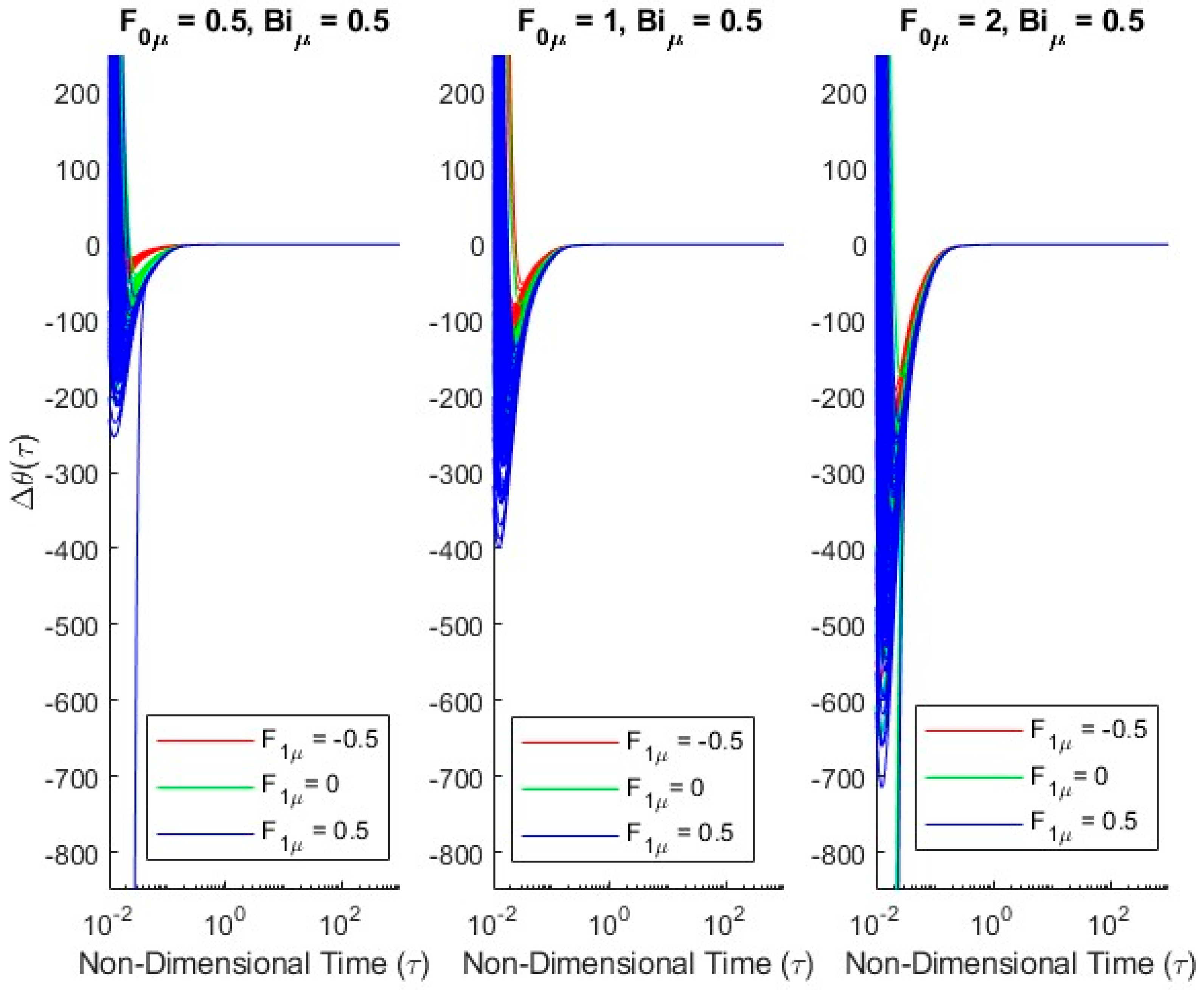
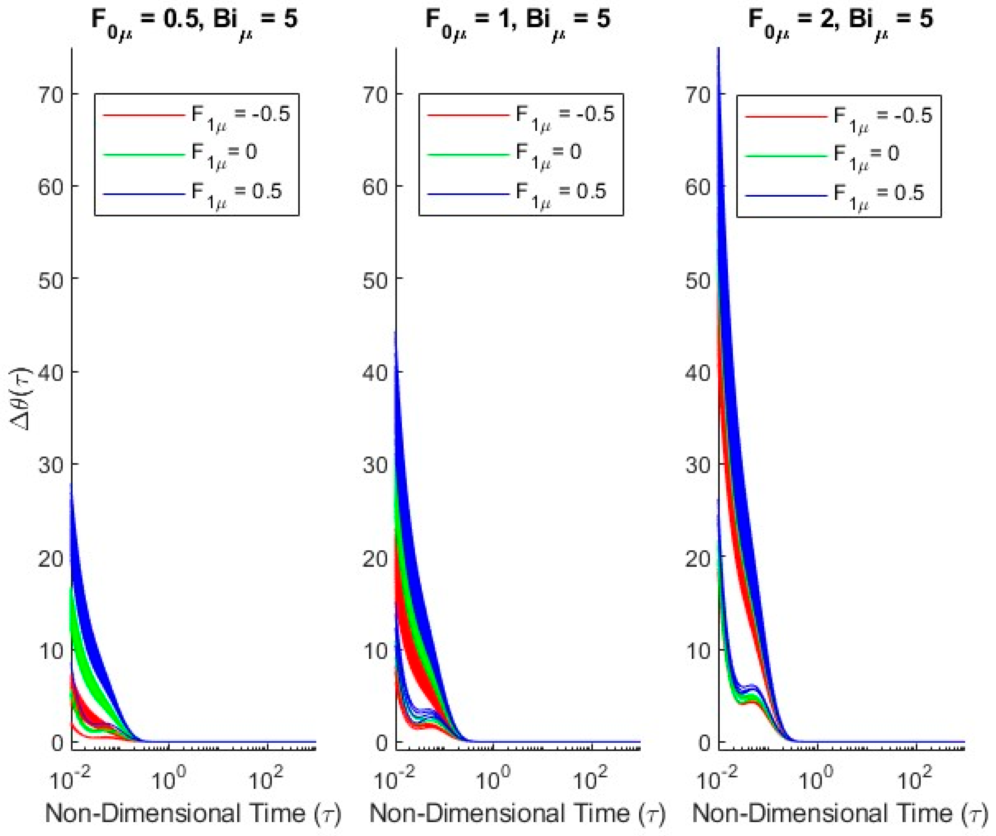
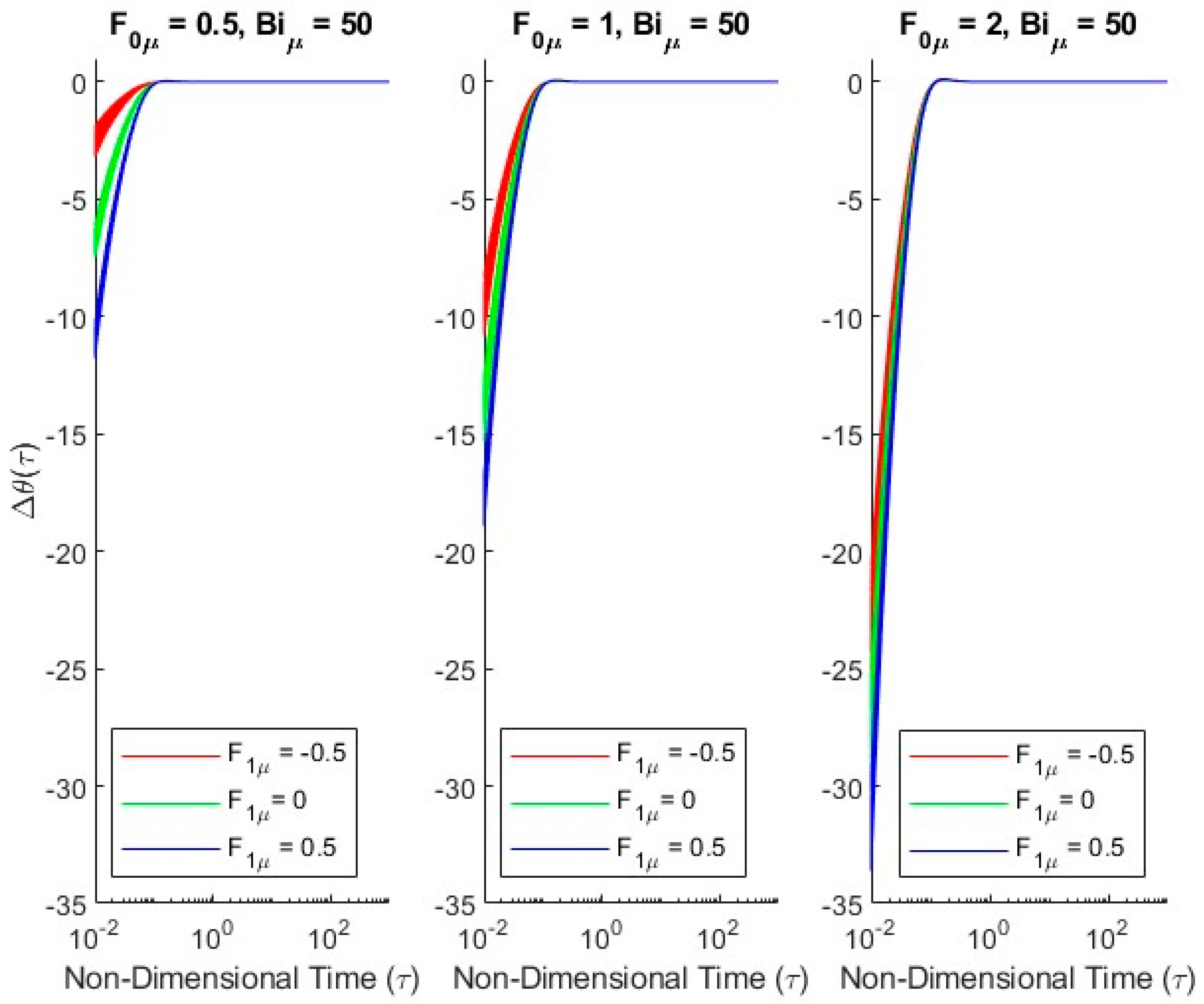
Figure 1, Figure 2 and Figure 3 display the non-dimensional temperature changes across the surfaces of the hollow sphere as non-dimensional time progresses. As the Biot number increases, the general behavior of the non-dimensional temperature differences follows a similar trend. The transient portion of this simulation for all cases lasts until a non-dimensional time of $\tau =1$. Beyond that point, there is a distribution of outputs, but it is much less than the uncertainty observed earlier in each simulation. Additionally, the distribution in the later portion of the simulation is approximately uniform.

We may compare simulations as $F_{0\mu }$ and $F_{1\mu }$ change individually. Across the 45 total simulations accomplished for $\Delta \theta$, as $F_{1\mu }$ changes, the stochastic spread changes very little. The different $F_{1\mu }$ values have a greater impact on the initial values of $\Delta \theta$, therefore affecting the transient path of the simulation. On the other hand, as $F_{0\mu }$ increases, the amount of uncertainty in the transient results also increases. This is most obvious when Biot numbers are small, such as $Bi=0.5$ depicted in Figure 1. In this case, the variation in $\Delta \theta$ increased from a range of about −0.5 to 0 for $F_{0\mu }=0.5$ to a range of about −2 to 0 when $F_{0\mu }=2$. This becomes less apparent as Biot number increases, and the magnitude of the Biot number itself drives the non-dimensional temperature change across the spherical surfaces. Increased stochastic spread in $\left(\mathbf{∆}\mathit{\theta }\right)$ or ${\mathit{\theta }}^{\mathbf{\prime }}(\mathbf{1},\mathit{\tau })$ could influence safety margins or material selection in aerospace design.

4.2. Non-Dimensional Heat Flux ${\theta }^{\prime }(1,\tau )$ at the Outer Surface

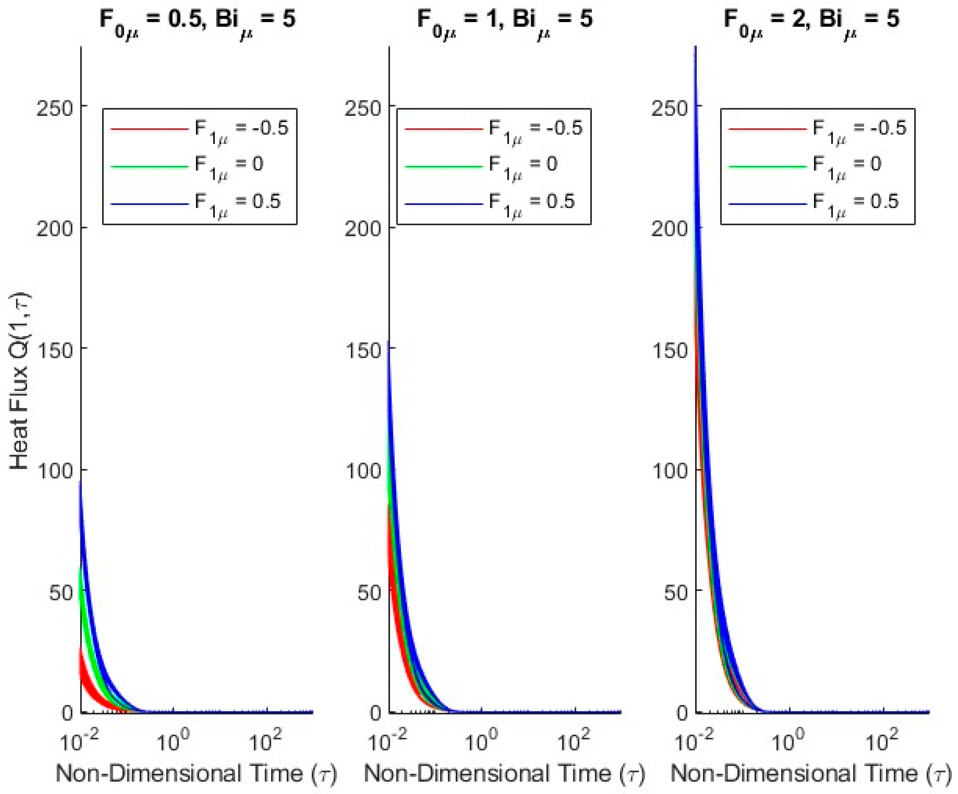
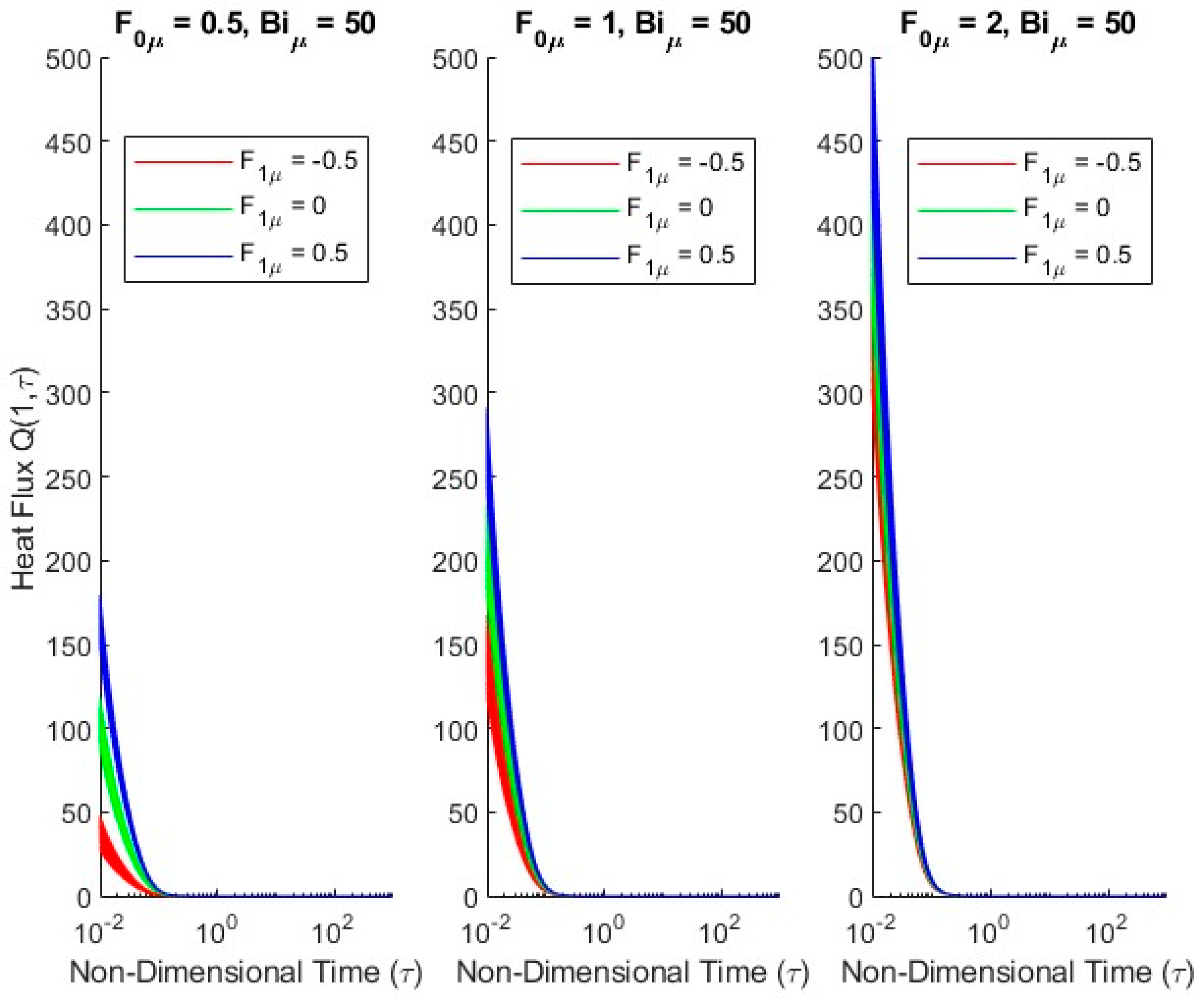
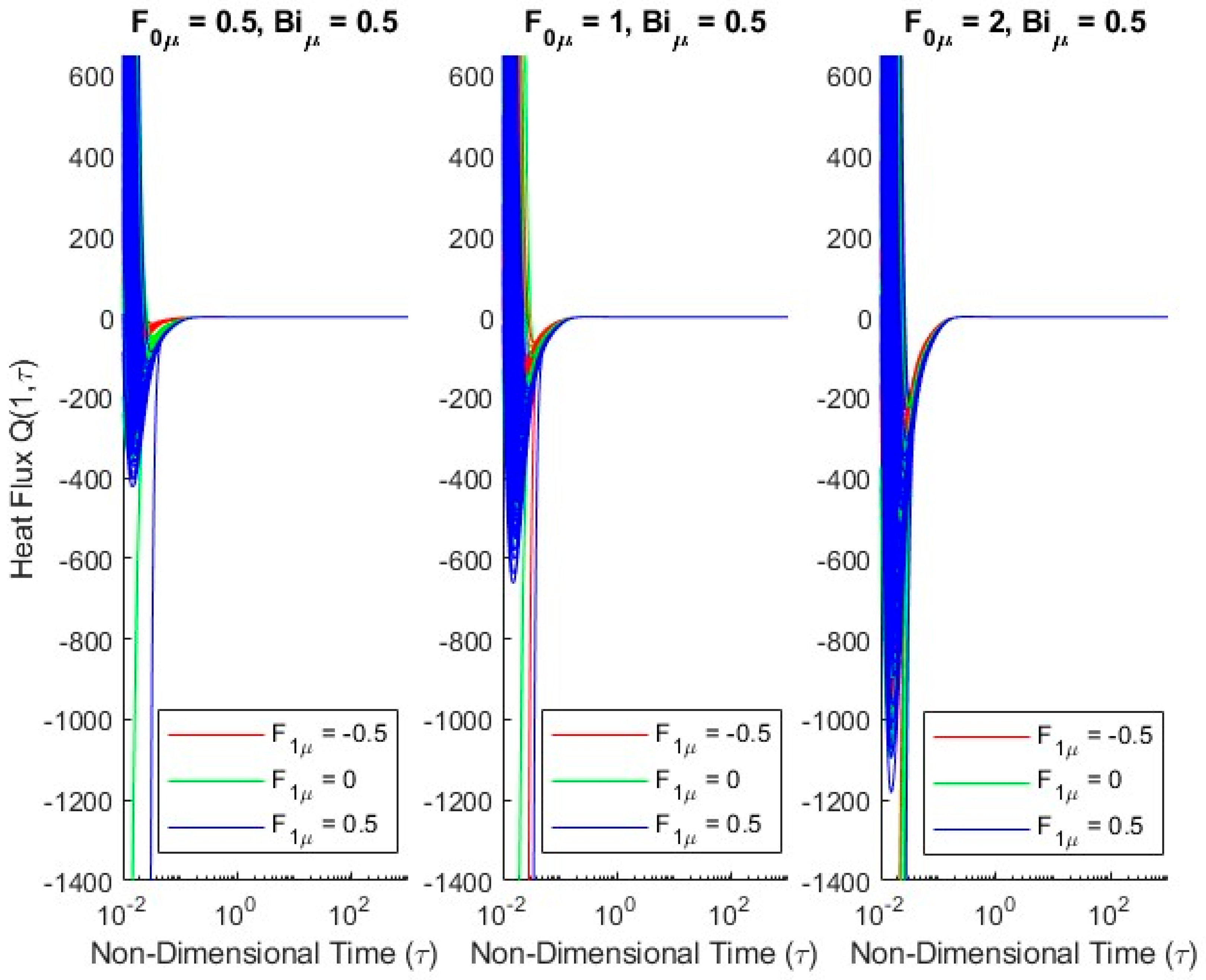
The parameters used for the non-dimensional heat flux are the same as those used in the non-dimensional temperature differences across the hollow sphere. Figure 4, Figure 5 and Figure 6 are laid out and organized in the same manner as seen above.

When observing the effect of $F_{0\mu }$ on ${\theta }^{\prime }\left(1\right)$, there is a much more noticeable change. With values of $F_{0\mu }=0.5$, the uncertainty in ${\theta }^{\prime }\left(1\right)$ is relatively low, and the general trend is an exponential decay with all negative values. With a value of $F_{0\mu }=2$, the uncertainty in ${\theta }^{\prime }\left(1\right)$ increases with an exponentially decaying trend. However, in this case, all values for ${\theta }^{\prime }\left(1\right)$ are positive. This suggests that the $F_{0\mu }$ term drives the direction of heat flux in these types of simulations.

For the third case ($B_i$ = 50) when $F_{0\mu }=0.5$, the simulations provide much more variation in the outputs. In fact, the uncertainty in the initial state of ${\theta }^{\prime }\left(1\right)$ is so great that the direction of heat flux may have different directions with all other conditions held the same. This quickly dampens out, and the final value reaches a constant when non-dimensional time $\tau =1$. This uncertainty in the direction of heat flux may have further implications when applied to a real-life system.

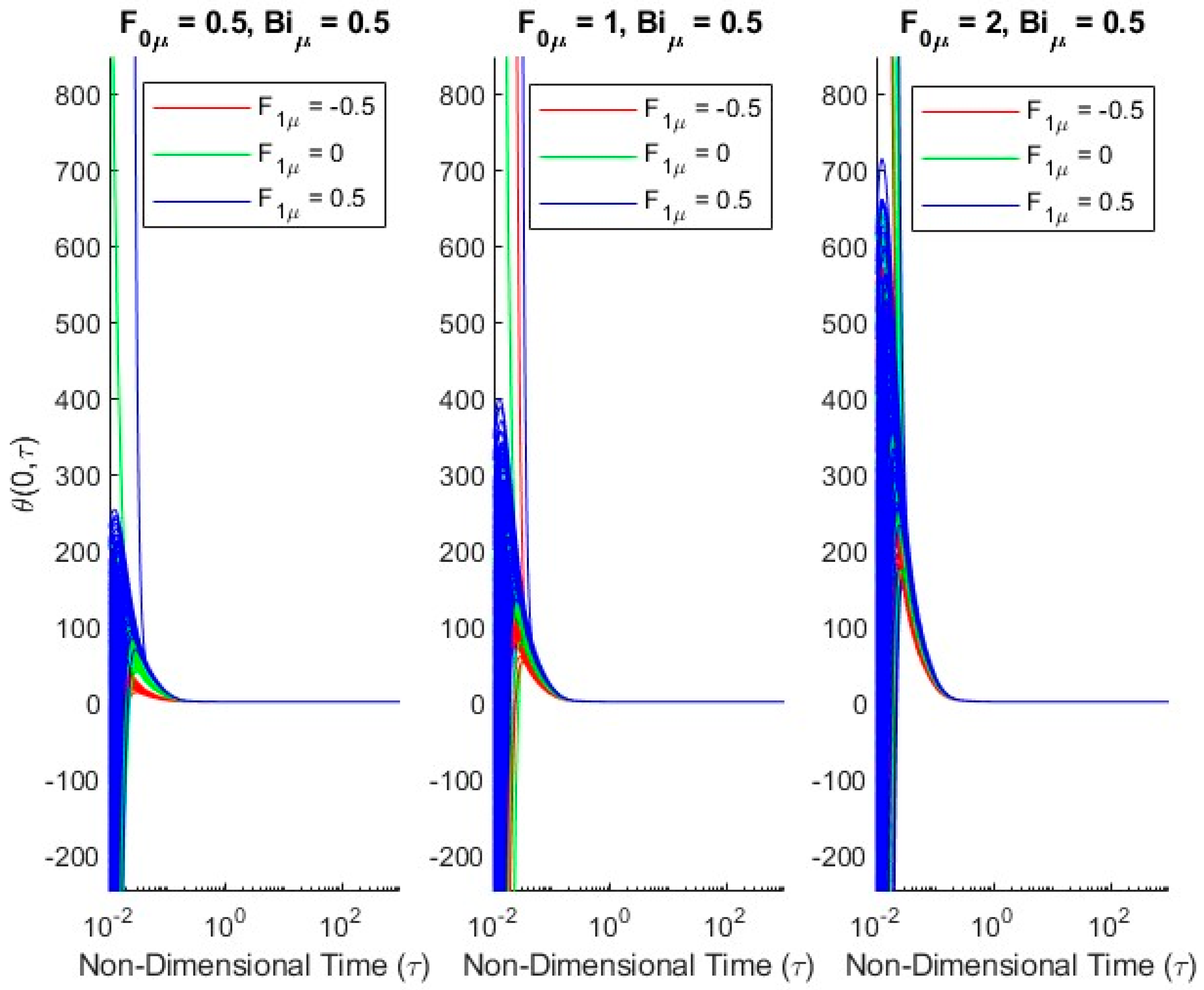
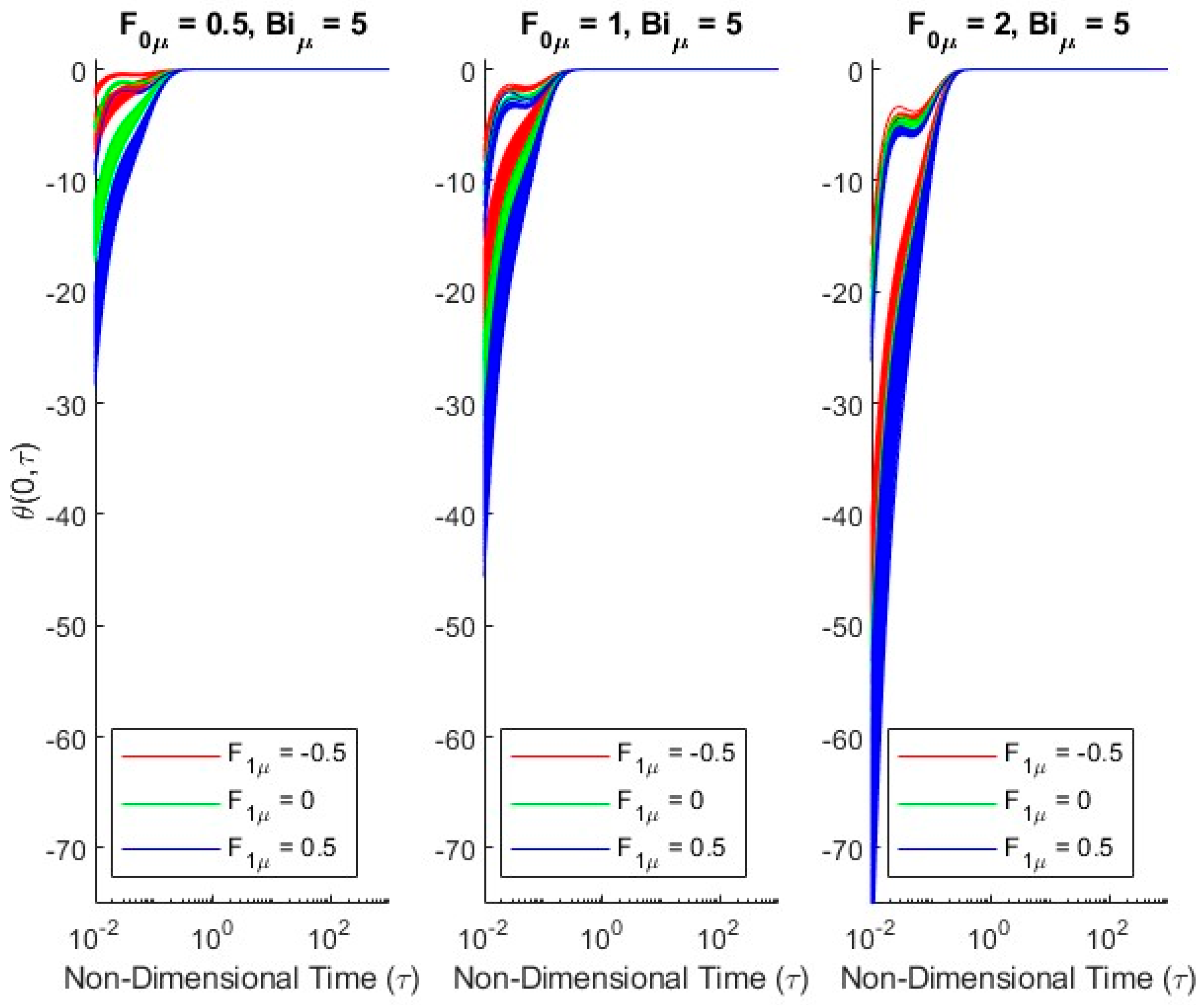
4.3. Non-Dimensional Temperature $\theta (0,\tau )$ at the Inner Surface

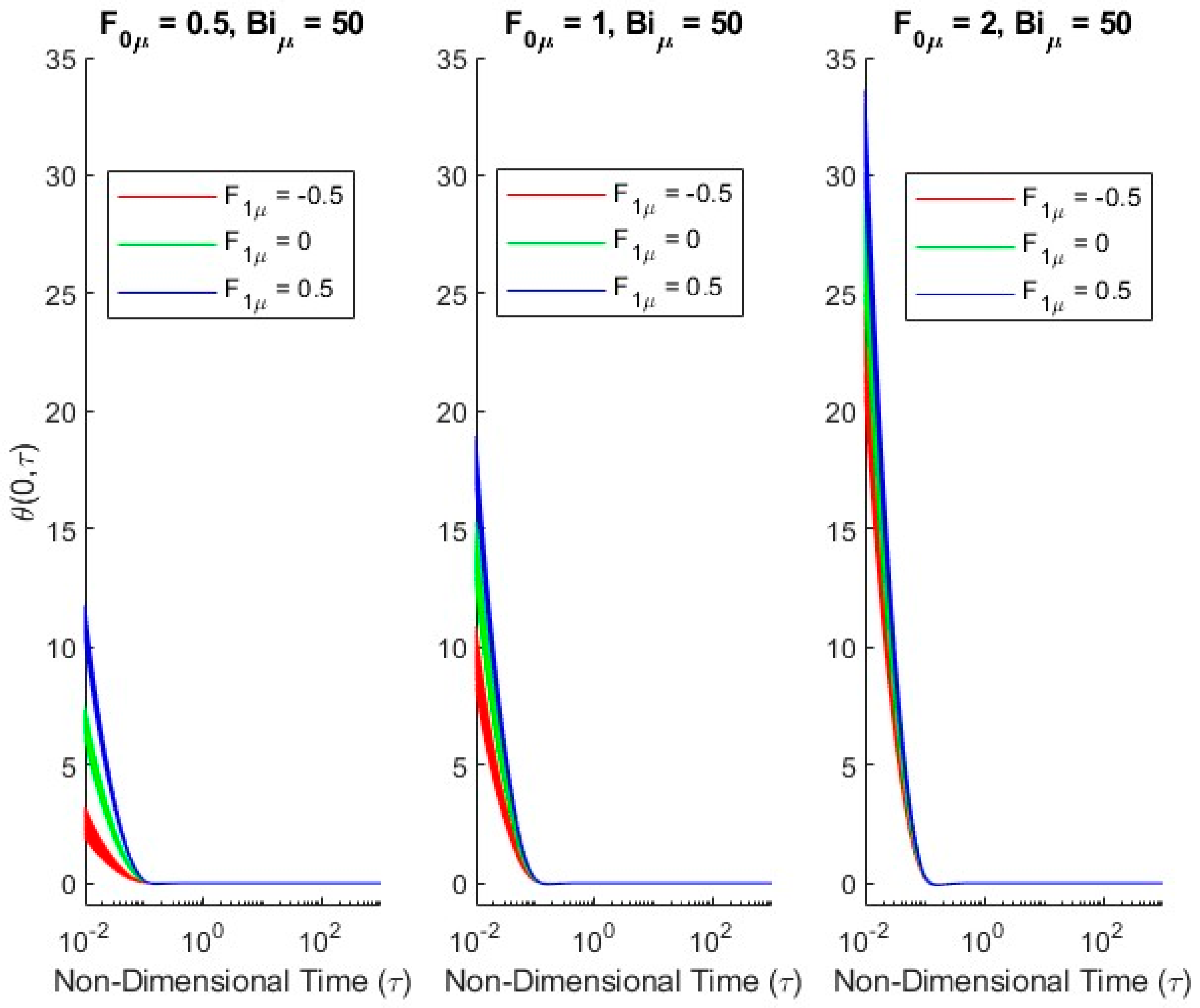
The parameters used for the non-dimensional temperature are the same as those used in the non-dimensional temperature differences across the hollow sphere. Figure 7, Figure 8 and Figure 9 are laid out and organized in the same manner as seen above.

However, in these simulations, the total uncertainty remains relatively consistent as the Biot number changes. The value of $F_{1\mu }$ has little effect on the overall uncertainty of the transient response but instead impacts the initial condition and path of the transients.

When observing the effect of $F_{0\mu }$ on $\theta \left(0\right)$, there is a much more noticeable change. With values of $F_{0\mu }=0.5$, the uncertainty in $\theta \left(0\right)$ is relatively low, and the general trend is an exponential decay with all negative values. With a value of $F_{0\mu }=2$, the uncertainty in $\theta \left(0\right)$ is high, with an exponential decay trend.

5. Concluding Remarks

After several Monte Carlo simulations for the one-dimensional hollow sphere system, the behavior of the transient thermal management properties was documented and displayed. Uncertainty in the Biot number and the initial conditions of each simulation affected the overall behavior of the interaction, but every simulation followed an exponentially decaying trend that ultimately reached a steady-state value with a small, uniform distribution.

The simulations that show the greatest variability in the values of $\Delta \theta$ are those with the highest values of $F_{0\mu }$, especially when the values of the Biot numbers are low. The simulations that show the greatest variability in ${\theta }^{\prime }\left(1\right)$ are those where the value $F_{1\mu }=0.5$.

This research can be extended to examine unsteady two-dimensional heat transfer cases for more practical application to real-life heat exchangers.

References

- Chapman, J.W. Development of Thermal Management System for Electrified Aircraft; NASA/TM-2020-220473; National Aeronautics and Space Administration (NASA): Washington, DC, USA, 2020.
- Li, K.; Liu, Z.; Xu, J.; Liu, S.; Wang, C.; Qin, J. Evaluation of High-Speed Aircraft Thermal Management System Based on Spray Cooling Technology: Energy Analysis, Global Cooling Multi Objective Optimization. Appl. Therm. Eng. 2023, 229, 120632. [Google Scholar] [CrossRef] [Scilit]
- Panasyuk, G.Y.; Yerkes, K.L. Input Uncertainty and Implication for Modeling Generic and High-Fidelity Transient Convection Problems. J. Thermophys. Heat Transf. 2022, 36, 739–748. [Google Scholar] [CrossRef] [Scilit]
- Panasyuk, G.Y.; Yerkes, K.L. Modeling of Uncertainty Propagation for Transient Heat Rejection Problems. J. Thermophys. Heat Transf. 2024, 38, 56–66. [Google Scholar] [CrossRef] [Scilit]
- Muff, J.D.; Gorla, R.S.R.; Forster, E. Uncertainty Quantification for Transient Thermal Management. J. Adv. Therm. Fluid Syst. Aerosp. 2025, 1, 9–17. [Google Scholar] [CrossRef] [Scilit]
- Gorla, R.S.R.; Forster, E.; Pentecost, B. Uncertainty Propagation in Transient Heat Transfer from an Extended Surface. Int. J. Turbo Jet Engines 2025, 42, 779–792. [Google Scholar] [CrossRef] [Scilit]
- Gorla, R.S.R.; Pentecost, B.; Forster, E. Quantification of Uncertainty Propagation in Transient Heat Transfer from Flux-base Extended Surface. Int. J. Turbo Jet Engines 2025, 42, 807–824. [Google Scholar] [CrossRef] [Scilit]