While there are multiple, common approaches to drive the Clapeyron equation, here we will make use the dimensionless (molar) Gibbs free energy,
, as a generating function [
1]. Starting with our definitions of
G:
and
we next work out the corresponding differential for the dimensionless (molar) Gibbs free energy:
which leads to the final expression:
Next, two simplifications are made. Starting with the first differential:
and then the second:
where:
Therefore:
Considering the general case of equilibrium between phases
I and
, at coexistence:
If the system were to remain in a state of equilibrium for a change in
T and
P, we have:
Collecting terms:
For the case of vapor–liquid equilibrium, let phase
be vapor and phase
I be liquid. This results in (one of several forms of) the Clapeyron equation:
2.1. Clausius/Clapeyron Equation
While the Clapeyron Equation (Equation (
14)) is rigorously correct, we next make a series of assumptions that will ultimately lead to the Clausius/Clapeyron equation commonly introduced in the undergraduate curriculum. This is motivated by
Figure 1, wherein a plot of
versus
appears linear from the triple point to the critical point [
1,
2,
3,
4,
5,
6], considering the case of water as an example [
7,
14]. We note that all of the figures included in this manuscript were prepared with MATLAB code available in the
supporting information accompanying the electronic version of this manuscript. While in this manuscript we only consider the case of water and hexane as examples, additional systems are provided as an example in the
supporting information.
On the right hand side, first we consider
. At low temperatures well removed from the critical point, it can be assumed the vapor phase is an ideal gas. For this case we take:
Further assuming that
is much greater than
such that
can be assumed negligible:
This is equivalent to assuming that
and the
is negligible. This results in the expression:
In general, undergraduate students are told that the assumptions are reasonable so long as we are well removed from the critical point [
1,
2,
3,
4,
5,
6].
Next, in order to integrate Equation (
17), the temperature dependence of
must be known. If we assume that
is constant over a temperature range of interest, we obtain the expression:
where
A and
B are positive constants, where:
where
is the reference temperature and
the reference saturation pressure at
, and:
Equation (
18) suggests that a plot of
versus
should be linear with a negative slope. This well explains the observation of
Figure 1. While most undergraduate textbooks acknowledge that the assumption that
and that
is negligible is only reasonable at low pressures well removed from the critical point, Equations (
18)–(
20) are typically the end point for discussion [
1,
2,
3,
4].
While this provides justification of the linear trend in
Figure 1, it is misleading and can cause confusion to the undergraduate student learning the material for the first time. At low pressures well removed from the critical point, it is reasonable to assume
. However, at the critical point where the two phases cease to exist,
. Therefore,
decreases with increasing temperature. Likewise,
is not constant as evident by the Watson equation typically introduced in the undergraduate curriculum [
15,
16,
17]. Below the critical point
, and at the critical point
. We therefore find also that
decreases with increasing temperature. Knowing this, the previous approach used to arrive at Equation (
18) is less than satisfying, even though it appears to agree with
Figure 1.
This shortcoming is acknowledged by two of the common undergraduate textbooks which we reviewed. Koretsky [
6] arrives at Equation (
18) using the assumptions listed earlier. However, he acknowledges that the error introduced by assuming
is constant (assumption 3) is approximately offset by the error introduced by assuming
is negligible and
(assumptions 1 and 2).
A further discussion is provided by Elliott and Lira [
5]. In that work the authors arrive at Equation (
18) using the assumptions listed earlier. However, this is followed in their textbook by Section 9.3 “Shortcut Estimation of Saturation Properties”. Here the authors mention that one may alternatively arrive at Equation (
18) by instead assuming that
is constant. Further, this assumption is reasonable over the range
, where
is the reduced temperature, where
is the critical temperature. The authors then use the critical point (
) and acentric factor (
) as reference points to solve for the constants
A and
B, to develop a predictive vapor pressure expression. We note also that the suggestion of assuming
is constant is also made in references [
17,
18]; however, these are references not typically used in undergraduate courses.
2.2. Updated Clausius/Clapeyron Equation Discussion
Here our motivation is to build upon the work of Elliott and Lira [
5], and present an alternative discussion and motivation for Equation (
18) to explain the linearity of
versus
. Within our discussion here we will consider the case of water and hexane, using reference data readily available from the “Thermophysical Properties of Fluid Systems” by NIST [
7]. MATLAB code used for all of the analysis and figures is provided in the
supporting information accompanying the electronic version of this manuscript, along with additional systems that may be used as an example. The goal of the MATLAB code is to provide a useful resource for undergraduate thermodynamics students.
It is our recommendation that one should start with the rigorously correct Clapeyron equation (Equation (
14)). From there, one need only introduce the single assumption that the ratio
is constant which allows one to obtain the integrated Clausius/Clapeyron equation (Equation (
18)), where now:
where
is the reference temperature and
the reference saturation pressure at
, and:
This is a simple update to the conventional instruction. This is motivated and reinforced to students in a series of simple plots.
First, in
Figure 2 and
Figure 3 we consider plots of
and
versus
T, and a plot of
versus
. The plots span the temperature range from the triple point to the critical point. As expected,
is positive, decreasing to a value of 0 at the critical point. Likewise,
at low temperatures, decreasing to a value of 0 at the critical point. We therefore see that it is not reasonable to assume
over the entire temperature range, nor is it reasonable to assume
is constant over the entire temperature range. However, the functional dependence of
and
versus
T are similar. Furthermore, the plot of
versus
appears to be linear, except near the triple point. Near the triple point, the rate of decrease in
is greater than
.
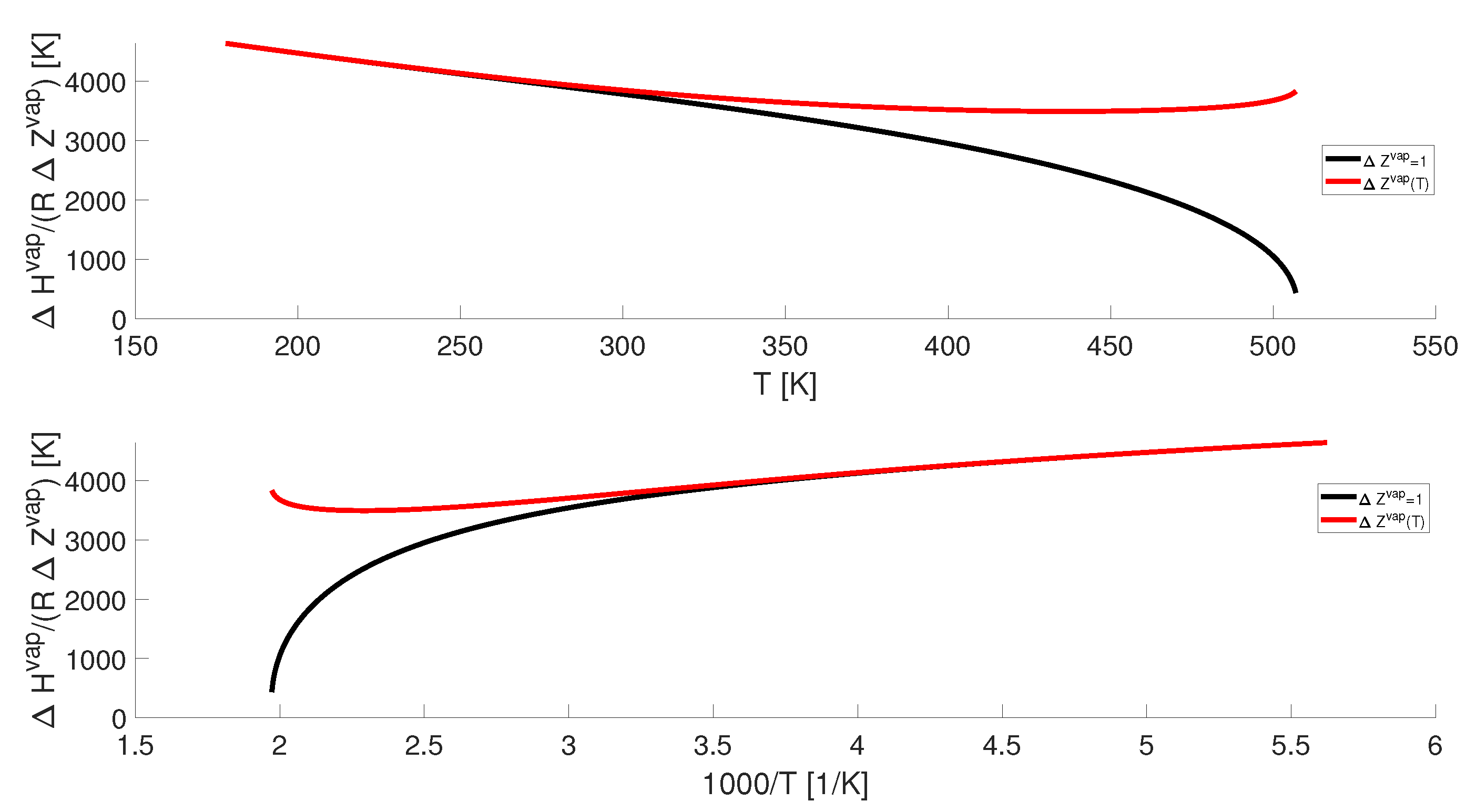
Next, in
Figure 4 and
Figure 5 we plot
versus
T and
from the triple point to the critical point. We compare the case where
, corresponding to the case of
, to the case where we account for the temperature dependence of
. We find that the range of values for
is significantly smaller than for
. While both
and
decrease with increasing temperature, the effect in
appears to cancel. We see that it is more reasonable to assume
is constant as compared to assuming
is constant.
This is further emphasized by the Watson plot in
Figure 6 and
Figure 7. In a Watson plot, we find that
versus
yields a straight line [
15,
16,
17]. In
Figure 6 we consider the case of
and
(where
) versus
. While
versus
yields a straight line as expected, we find that
versus
appears nearly constant. We do observe curvature near the triple point, but in general
appears constant over a wide range of temperatures.
As our final example, we return to our starting point of the Clapeyron equation (Equation (
14)), then separate and numerically integrate the resulting expression. Integrating from a reference temperature (
) and corresponding reference pressure (
):
In order to evaluate this expression, one must know the temperature dependence of
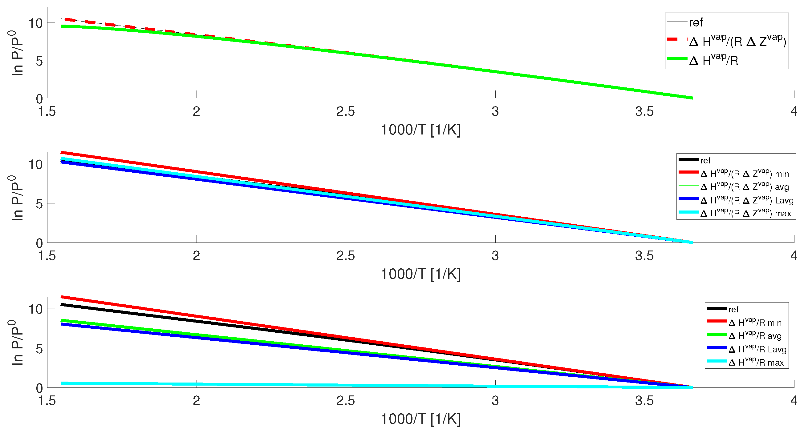
. Fortunately, tabulated data are readily available from the “Thermophysical Properties of Fluid Systems” by NIST which can be numerically integrated and compared to the reference vapor pressure data. In the top pane of
Figure 8 and
Figure 9, we numerically integrate two sets of temperature-dependent data and compare to reference vapor pressure data, taking our reference state to be the triple point. In the first case, we set
, which corresponds to numerically integrating
. The predicted data match the reference vapor pressure at the triple point by construction, but diverge at the critical point due to propagation of errors and the assumption of
breaks down with increasing temperature. Clearly then,
is important for accurate calculations. In the second case we numerically integrate
. The resulting predictions match the reference data as expected.
Following this, in the middle pane we consider the case of assuming is constant. For the value of we compare the use of the value at the lowest temperature (the triple point, min), the average value (avg) and the average (natural) log value (Lavg), and the value at the highest temperature (just below the critical point, max). We find that the use of the average and average log value result in excellent predictions that appear to overlap the reference data. The use of the value at the highest temperature also performs exceptionally well. The performance with the minimum temperature is the worst; nonetheless, the predictions are still very good considering they require only knowledge of at the triple point.
Lastly, in the bottom pane, we consider the case of assuming and assuming is constant. For the value of we again use the value at the lowest temperature (the triple point, min), the average value (avg) and the average (natural) log value (Lavg), and the value at the highest temperature (just below the critical point, max). Interestingly, the best set of predictions is made using the value at the triple point. At the triple point, the assumption that is reasonable, and we find that the predictions using a constant value of and at the triple point are indistinguishable from each other. The other predictions noticeably diverge from the reference data, with the predictions worst using the value of at the highest temperature where the assumption that is least appropriate.


