


Abstract
Uncertainty quantification in science and engineering has become increasingly important due to advances in computational mechanics and numerical simulation techniques. In this work, the relationship between uncertainty in soil material parameters and the variability of failure loads and displacements of a shallow foundation is investigated. A Drucker–Prager constitutive law is implemented within a stochastic finite element framework. The random material variables considered are the critical state line slope c, the unload–reload path slope , and the hydraulic permeability k defined by Darcy’s law. The novelty of this work lies in the integrated stochastic u–p finite element framework. The framework combines Drucker–Prager plasticity with spatially varying material properties, and Latin Hypercube Sampling. This approach enables probabilistic prediction of failure loads, displacements, stresses, strains, and limit-state initiation points at reduced computational cost compared to conventional Monte Carlo simulations. Statistical post-processing of the output parameters is performed using the Kolmogorov–Smirnov test. The results indicate that, for the investigated configurations, the distributions of failure loads and displacements can be adequately approximated by Gaussian distributions, despite the presence of material nonlinearity. Furthermore, the influence of soil depth and load eccentricity on the limit-state response is quantified within the proposed probabilistic framework.
1. Introduction
Determining the bearing capacity of shallow foundations, together with the associated stress and displacement fields, is a fundamental problem in geotechnical engineering. Starting with the work of [1], who proposed the ultimate load of soils as a function of soil depth, friction angle, and total soil density, several subsequent studies extended this research: [2,3,4,5,6]. Most existing studies investigate the failure surface using the Mohr–Coulomb constitutive model combined with linear elastic analyses. Most investigations employ one- or two-dimensional meshes, considering either homogeneous soils or stratified soil profiles [7,8]. Scientific developments were incorporated into regulatory texts for settlement analysis through the definition of variables N (accounting for friction) and variables S (accounting for settlement shape). Following this, the variables , , and , , are defined. Subscripts q, c, account for the three factors that define the ultimate load, namely the effect of present vertical uniform force in the lateral of the foundation, the soil cohesion, and the settlement dimensions combined with the total weight of the soil, respectively [9,10,11].
Several studies have investigated the variability of bearing capacity in saturated porous continua. These studies relate footing settlement response to uncertainty in input material parameters using stochastic finite element analyses. The input randomness may be simulated in two alternative ways. One methodology suggests that the properties of nodal points are modeled following random variables. Then, shape functions are used for the estimation of the material parameters inside the element. The shape functions are deterministic relations [4,12,13,14,15,16,17,18]. An alternative methodology is constructing a random field representation. Algorithms like the Karhunen–Loève, spectral representation, or the spatial average method may be implemented. With this approach, the material input randomness may be presented in a more realistic way [19,20,21,22,23,24,25,26,27,28]. The sampling selection can be performed through non-biased pseudorandom methodologies, or an importance sampling algorithm may be adopted, like sampling through Latin Hypercube (LHS) [29,30]. Following sampling selection and the determination of input parameters, the Monte Carlo analysis may take place.
Precedent works correspond to 1D-2D elastic halfspace analysis with material law using the Mohr–Coulomb constitutive model. In the proposed work, a stochastic model with a Drucker–Prager constitutive law is adopted, which is a model considered reliable for cohesionless soil in terms of stresses and strains estimation in different applications of geotechnical engineering such as shallow foundations or landslides [31,32,33,34]. This constitutive model within a finite element model may reliably demonstrate the stresses, strains, displacements, and loads fields in all loading occasions. The standard Monte Carlo simulation method computational cost may be reduced with computational algorithms as proposed in [35,36]. The bearing capacity determination is performed through a recurrent algorithm proposed and reformatted by the author [37,38]. This algorithm results in valid failure loads with one initial guess and a small number of convergence trials. The recurrence relation is defined, confirmed, and contrasted with the classic bisection algorithm. The main objective of this work is to quantify uncertainty in footing settlement behavior. Specifically, the variability of failure displacements and load responses is examined. Moreover, the randomness of the failure curve in relation to the randomness of the input variables such as the soil depth and the spatial relation of the material soil parameters is also presented. Finally, this work aims to apply the recurrence algorithm derived from the authors of the cited publications in order to speed up the stochastic analyses.
The random material parameters adopted are the variable for compressibility , the hydraulic conductivity factor k, which is the permeability in speed units, and the critical state line slope c of the soil. The shape functions of the material parameters in terms of the depth z of the soil are linear and include the constant function and the random field functions, originating from Karhunen–Loève sum application with the adoption of an exponential autocorrelation relation. In the constant and linear spatial distribution, the truncated normal random variable [39,40] is the random variable probability density function considered at the nodes. The LHS importance sampling algorithm is used to select the input uncertain values. The eccentricity of the foundation and correlation lengths are the parameters and are compared to the respective solid analysis, namely when the pore pressure is not present.
2. U-P Finite Element Formulation
In the event of a porous continuum subjected to static and dynamic forces, the displacements and the pore pressure at nodal points may be found using the Biot partial differential system. If the momentum of the loads is of small velocity or quasi-static conditions are evident, the mathematical system may be transformed into a less computationally expensive system. The so-called u–p formulation consists of a system of ordinary differential equations describing fluid–solid momentum balance and water flow governed by Darcy’s law, combined with strain–stress relations and boundary conditions. In this article, this formulation is selected since static loads are subjected to cohesionless soil continua.
The finite element formulation of the u–p problem is the following:
whereas
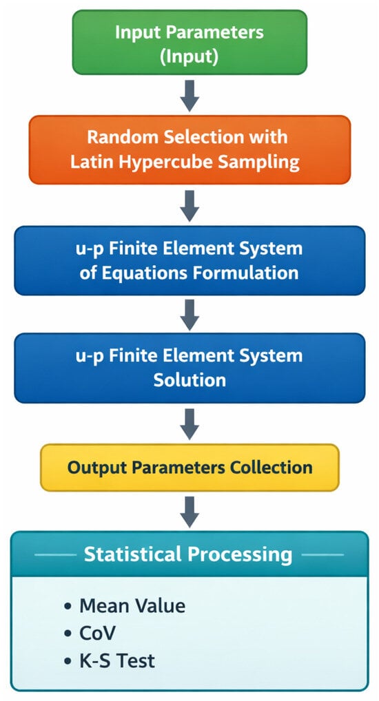
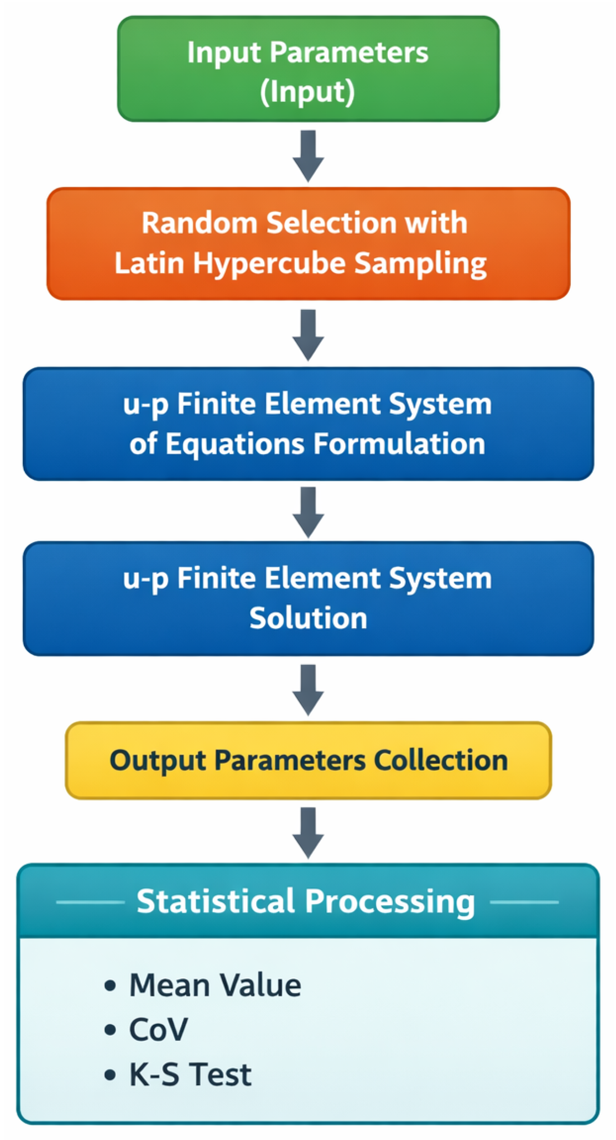
is the matrix containing the permeability coefficient in each global direction, is the gravitational forces in terms of the total density of the soil continua, and is a function of bulk modulus of both pore fluid substance and soil skeleton. represents the matrix of shape functions. are the mass, damping, and stiffness matrices influenced by the soil skeleton only. are the matrix for coupling the equations of the u–p formulation, the matrix for permeability in terms of forces, and the matrix for quantifying the saturation of the soil skeleton. represents the loads that correspond to the forces applied externally. Time integration of the coupled equations is performed using standard solution schemes, such as the Newmark direct integration method. The aforementioned u–p formulation is randomly influenced by the random variability of the material properties of the compressibility factor, critical state line inclination, and permeability. The u–p formulation is solved once per Monte Carlo realization. Each realization yields a set of output parameters for statistical analysis. Subsequently, the statistical moments estimations and moments are performed and discussed. A schematic representation of the algorithmic procedure of this study is given in Figure 1.
Figure 1.
Graphical representation of the methodology of the present study.
3. Drucker–Prager Material Constitutive Model
For predicting failure from a stress–strain perspective, a constitutive material model must be defined. For cohesionless soils, one usual yield criterion is the Mohr–Coulomb function in principal stress systems. However, the Mohr–Coulomb model has two main limitations. Its performance is reduced under dynamic loading conditions. More importantly, the pyramidal yield surface contains sharp corners, which makes the yield function non-differentiable and causes numerical instability. This may lead to numerical instability when the Mohr–Coulomb criterion is used to derive the constitutive matrix at the integration point level. This is clearly a numerical problem rather than a physical abnormal behavior, thus a smoother function is more applicable. In stochastic analysis this is also evident [41]. In particular, in the present study, the mean number of iterations using the Mohr–Coulomb constitutive model for a deterministic failure analysis is about 10, while in the case of the Drucker–Prager constitutive model, the respective number is about 5 iterations. In addition, the maximum number of iterations for convergence for the Mohr–Coulomb model was up to 100, while for the Drucker–Prager model it was up to 15. Therefore, in Drucker–Prager simulations the variation in the number of iterations in each load step is smaller. Furthermore, the mean computational cost for a deterministic simulation of this work in the case of the Mohr–Coulomb model is 45 min. The corresponding cost for the Drucker–Prager model is 27 min. Consequently, a computational cost reduction of approximately 40% is achieved. Therefore, the Drucker–Prager model is more applicable for numerical stability and computational cost.
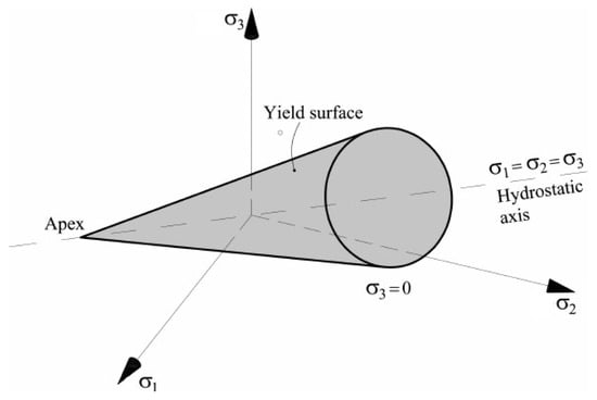
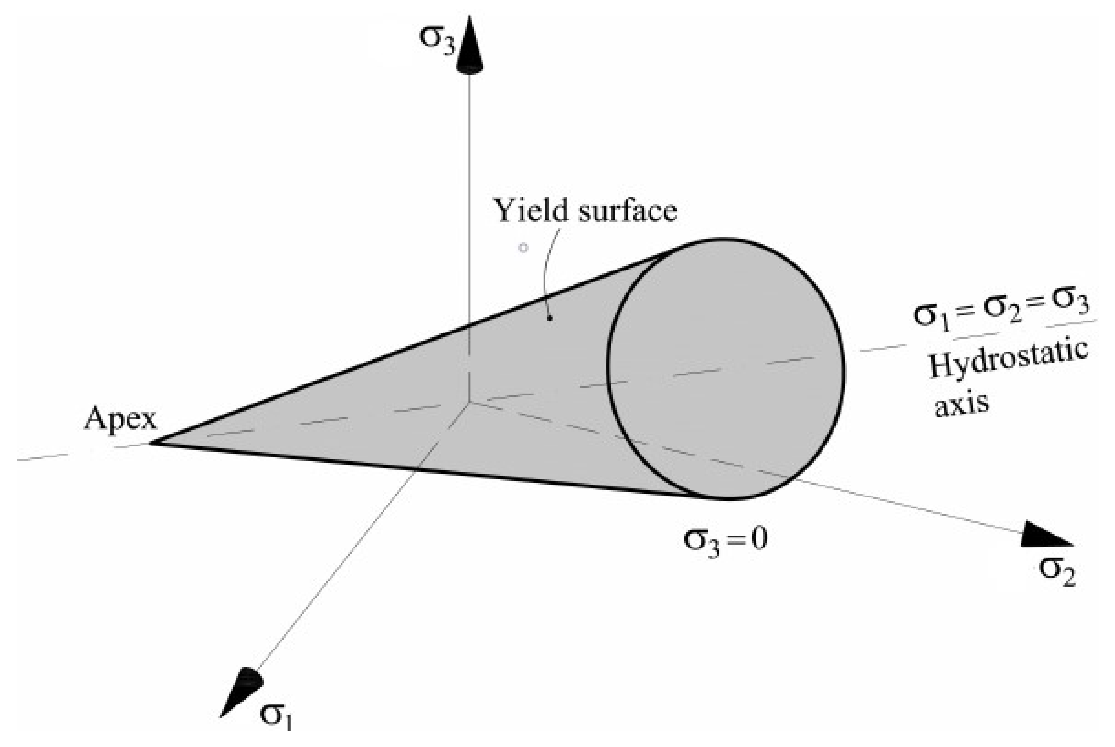
To overcome this difficulty, the Drucker–Prager material yield function is adopted. This function is a cone shaped 3D curve. The instabilities are reduced to only an apex of the curve. However, even in this case a constitutive matrix is easily obtained. This constitutive model is hydrostatically dependent, unlike the Von Mises function but similar to the Mohr–Coulomb criterion. It is applicable to brittle material in static and dynamic loading. Its coefficients are either experimentally found or selected to fit the Mohr–Coulomb pyramid, internally or externally. Finally, other critical points may be selected, like uniaxial compression, so that the Drucker–Prager cone may fit. In general, the main parameters sufficient for coefficient derivation are cohesion , the friction angle , and the dilation angle , and are denoted by . The main equations and a schematic representation of the Drucker–Prager law are given below in Equation (5) and Figure 2. It should be noted that the elasticity law is the isotropic poroelasticity, to which bulk modulus is given by , where is the specific volume, is the hydrostatic stress component, and is the unload–reload curve slope.
Figure 2.
Graphical representation of the Drucker–Prager yield stress model in 2D principal stresses plane.
4. Stochastic Representation for Input Uncertainty
In the stochastic finite element method, an important counterpart of the analysis is the consideration of the randomness of all input variables. Namely, for each parameter a function
is to be assumed, where stand for the input space and possible time vector, or else the deterministic parameters of the problem and the probability parameter of the function, respectively.
This function may be constructed using two possible approaches. In the first approach, this function can be a sum of products of deterministic functions multiplied by a set of univariate probability density functions
where are the deterministic shape functions of the classical finite element approach and the set of one-dimensional probability density functions for the uncertainty considered at the nodal points of the element. The shape functions may not be the ones used for the displacements of the finite element approach, should the uncertainty of the spatial distribution be adopted in another way.
The second approach is the consideration of the classic random field approach. In this case, the function f could also be a sum of products of deterministic and stochastic counterparts. However, this may not be the case in some other approaches, such as the spatial average method, in which the random field is transformed into a set of random variables, each one containing the spatial average of some realizations. In this article, the Karhunen–Loève truncated series are employed. Each function is formulated as follows
In this equation is the mean value, and are the eigenvalue and eigenfunction j, respectively—the solution to the integrodifferential Fredholm problem with defined autocorrelation function . Finally, are a set of standard normal random variables whose cross-correlation is zero.
In this article, both approaches are implemented for input randomness. For the first approach, the shape functions coincide with the ones for the standard finite element approach. For the univariate probability density function, the one corresponding to the truncated normal random variable is employed:
where correspond to the univariate standard deviation of the nodal point and the cumulative density function estimated at the beginning and the end of the subspace .
Finally, for the second approach, the Karhunen–Loève series expansion is selected. The integrodifferential Fredholm equation is solved using the exponential autocorrelation function, namely
The choice of the sampling procedure strongly influences probabilistic integration. It affects both the representation of input uncertainty and the accuracy of output statistics. To this extent, this procedure may be implemented by using fair coin random selection algorithms. However, for speeding up the procedure of crude Monte Carlo analysis, the sampling may be non-uniform and consider the importance of each subspace of the total probability space. One typical importance sampling method, which is implemented in the present work, is Latin Hypercube Sampling. This method is summarized in the following steps:
- Let us assume a random vector .
- For each do the following:
- –
- Break the subspace of the probability space into sub-intervals;
- –
- From each sub-interval choose a , and through the inverse of the cumulative function , find .
- End the loop for and sub-intervals.
- The random vectors are obtained as a random permutation of the sub-intervals for all .
This confirms that for all subsets of the Euclidean subspace of random variables and sub-intervals, exactly one sample will be taken.
The selection of this method for this work is because two major advantages are encountered. It has been confirmed that a smaller number of samples is needed to integrate the probability, thus the required computational expense is reduced. In addition, all possible types of sub-interval construction, as well as cross-correlation types, may be chosen for dealing with material parameters which are cross-correlated. In the present work, the Equations (6)–(9) are implemented to influence the material parameters of unload–reload slope, the critical state line slope, and the hydraulic permeability. Through them, the matrices of inertia, stiffness, and damping, as well as the equivalent forces of Equation (1), are stochastically affected. The sampling procedure is based on the Latin Hypercube Sampling method, which significantly accelerates the Monte Carlo simulations performed in this study.
5. Application of the Proposed Framework: Limit-State Estimation of Shallow Foundations with Uncertain Material Parameters
5.1. Research Methodology and Problem Description
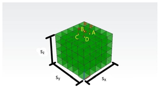
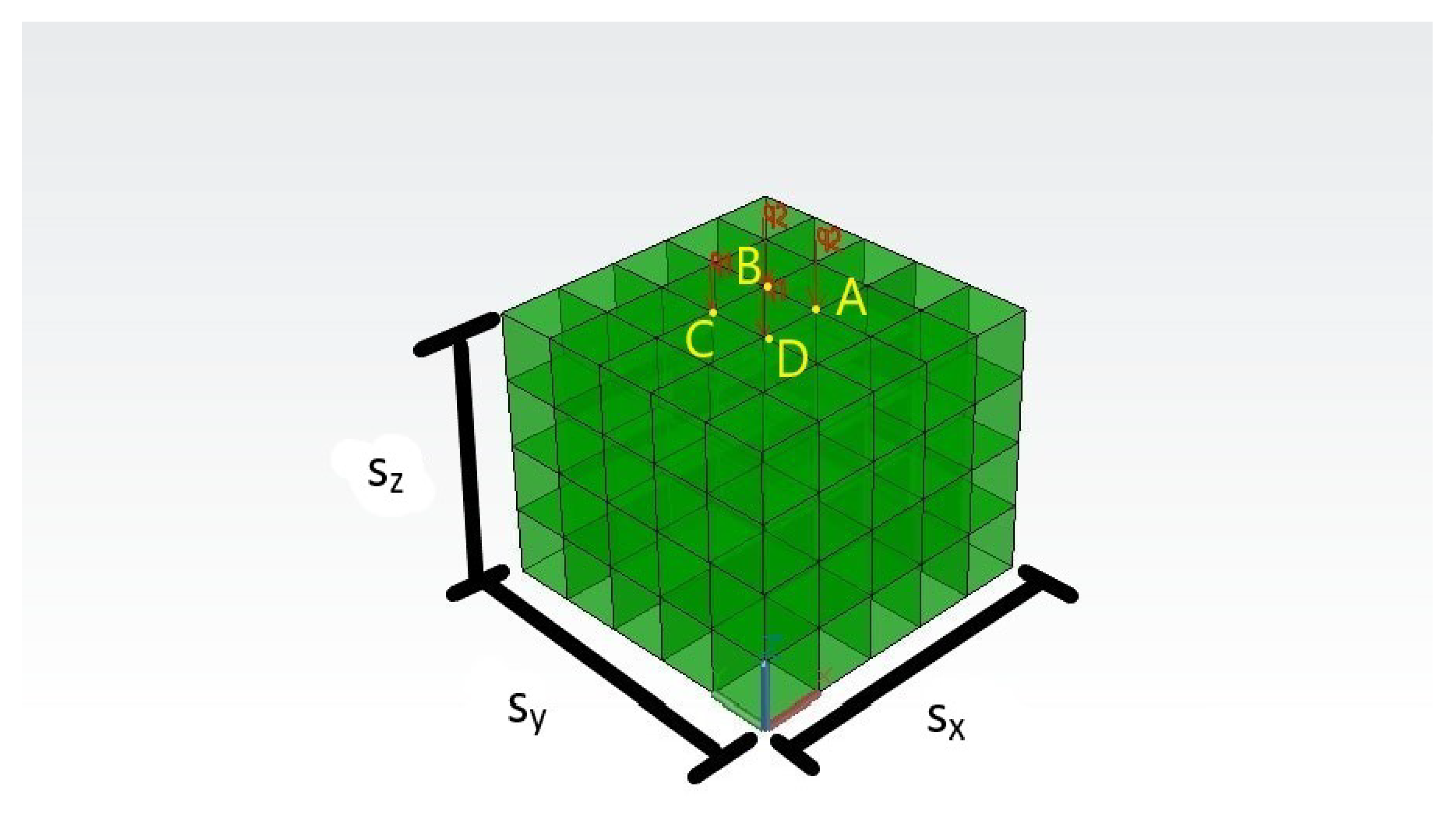
The proposed theoretical framework is applied to the soil continuum shown in Figure 3, which is governed by the coupled equations presented in Equation (1). Outputs of the simulations correspond to the ultimate stress of the foundation, by using a linear function with respect to the settlement area; the shallow foundation normal force; the ultimate foundation settlement, defined as the mean output of the A and B points of Figure 3; and the smallest foundation displacement, defined as the mean output of the C and D points of Figure 3. The nodal loads at C and D points and at A and B points denote the energy substitute nodal forces of a linear force distribution for an known eccentricity of the shallow foundation area. The , namely, the eccentricity is assumed as 0.0, , where is the foundation dimension corresponding to the eccentric load. The finite element model consists of eight-node hexahedral elements with linear shape functions for both displacement and pore pressure fields, as dictated in [42,43]. The soil continua length in X, Y, Z global vectors are, correspondingly, = 5.0 m, = 5.0 m, and = 4.0 m. The geostatic stresses are adopted as initial stresses vector , = 100 Kpa, which corresponds to the centroid of initial stresses of the soil point. The simulation of loading takes place over the duration of one day, and thus the conditions are static, with a time interval of 0.001 days. In Table 1, the soil continuum deterministic variables are given.
Figure 3.
Soil continuum representation ( = 5 m, = 5 m, = 4 m and ).
Table 1.
Soil continuum deterministic variables following [44].
is the initial specific volume of the soil, which leads to a void ratio of 0.6270. Boundary relations are . In the rest of the surfaces of the boundary, no constraints are imposed. The explanation regarding this selection of boundary conditions is the following. In this work, as a result of load and soil geometry, the computational domain that is outside the area of forces is more than twice the width of the area of settlement. It has been demonstrated in finite element simulations that this is sufficient to reliably calculate the failure load and respective displacements in the foundation area. The drainage conditions in boundaries are neglected since it is confirmed that in the nodes of the foundation area the displacements and pore pressure time response are practically the same. In addition, the analysis is static and the pressures have been fully dissipated. The plastic hardening slope is a deterministic parameter of a value of 1 kPa, in order to simulate perfect plasticity without brittle failure before the maximum strain exceeds the value of 0.001. The material parameters that are stochastic are the reload slope , the critical state line slope c, and the hydraulic value k comprising the water to soil permeability.
In the present study, the spatial representation of the material properties may be considered as a linear, constant, or stochastic process made by a Karhunen–Loève truncated series. The constant and linear representations for the unload–reload slope are adopted as the most common assumptions for the soil spatial interpretation. The same assumptions are made for the critical state inclination and the permeability of the Darcian flow. The comparison was made with the random process Karhunen–Loève series realizations, which do indicate the importance of spatial variability. The justification for the selection of the spatial representation of the material properties is as follows. The compressibility factor may be adopted as constant over depth following refs. [1,45]; Terzaghi was the first to adopt this selection. Therefore, a baseline analysis for comparison could be to adopt as constant over depth. The unload–reload slope may be considered linear following refs. [46,47]. This representation is a baseline analysis for interpreting the soil stiffening as the depth increases. Finally, could be a random field with a Karhunen–Loève series sum, following refs. [48,49]. The critical state line inclination may be adopted as constant, following refs. [50,51], as Schofield was the first to adopt this selection. Therefore, a baseline analysis for comparison could be to adopt c as constant over depth. Furthermore, c may be modeled as linear, following ref. [52]. This representation is a baseline analysis for interpreting the soil strength increase as the depth increases. Finally, c could be a random field with a Karhunen–Loève series sum, following refs. [53,54]. The permeability may be adopted as constant, following ref. [1], as Terzaghi was the first to adopt this selection. Therefore, a baseline analysis for comparison could be to adopt k as constant over depth. Finally, k could be a random field with a Karhunen–Loève series sum, following ref. [48,55]. This type of random field representation is used widely to uncertainty quantification studies, as a comparison to constant and linear representations to investigate the sensitivity of spatial randomness to uncertainty of the output parameters of the problem examined. It is shown that random fields are convenient to quantitatively assess the relation between random inputs and outputs in geotechnical engineering.
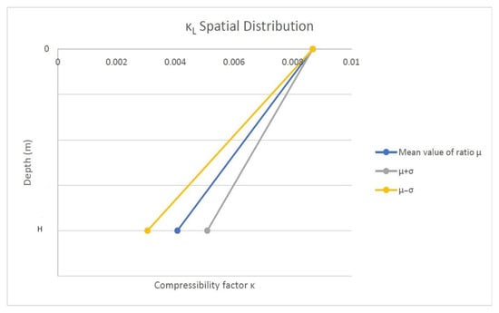
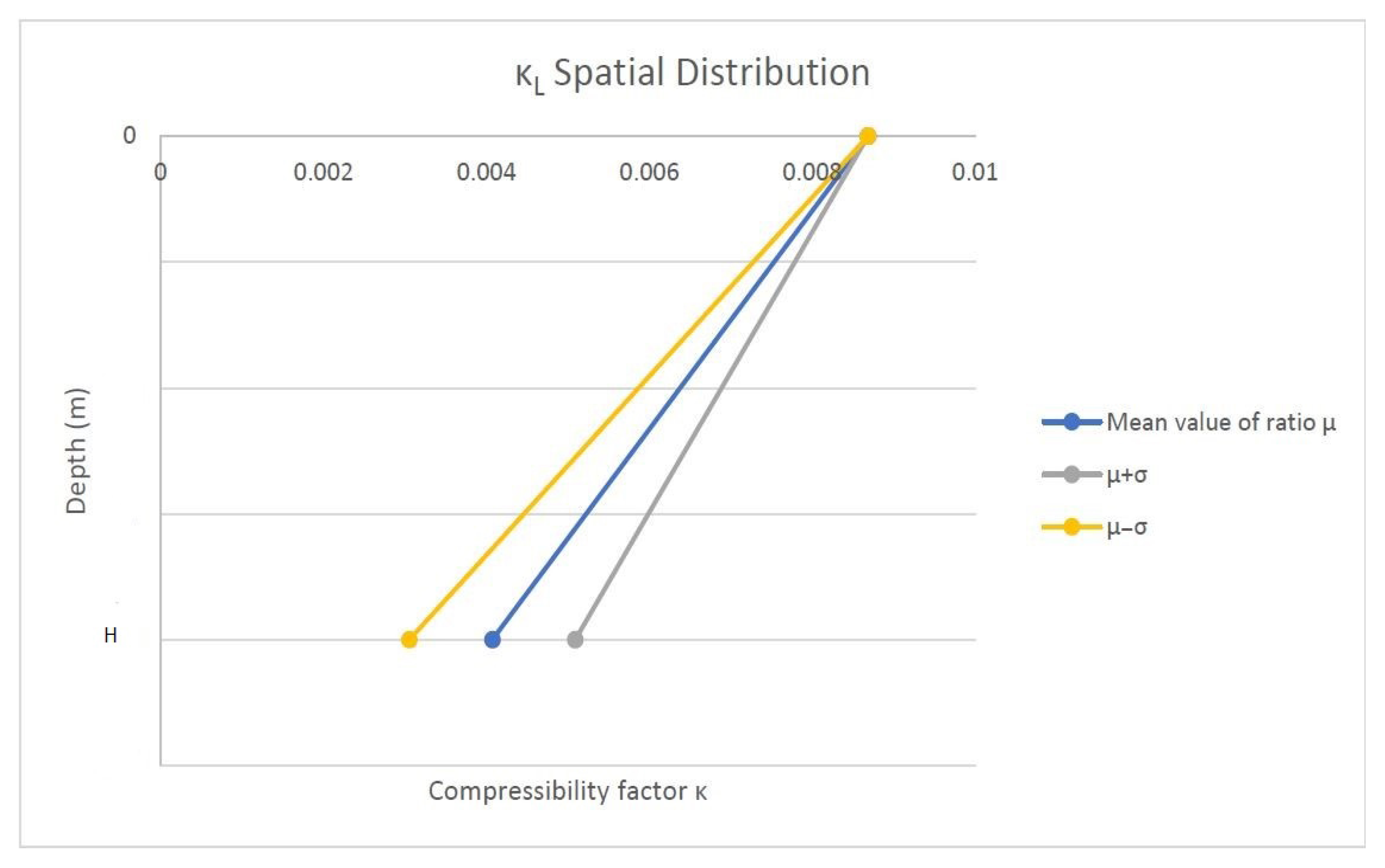
Considering the reload curve slope , the function with respect to depth may be adopted in the present work as linear (), or constant (). When is considered, and is assumed to follow the truncated normal distribution. The statistical moments of the ratio are when CoV is 0.25 and . Consequently, soil continua corresponds to a mean shear velocity of 200 . Figure 4 depicts the case. The bulk and the shear moduli are proportional, because Poisson ratio is considered constant and and shear veloctiy are connected. If is constant, the statistical moments are as follows: mean value is and CoV is 0.25.
Figure 4.
Illustration of the linear function for the unload–reload path slope with respect to depth.
Regarding critical state slope c, the constant function with respect to depth is used. There are two considerations with regard to the absolute value. When a random variable is adopted, , , namely the friction angle, is a truncated normal random variable PDF with the mean value and standard deviation , resulting a random vector for , accounting for middle stiffness cohesionless soils. Components of are taken from the Latin Hypercube Sampling methodology explained in Section 4. Afterwards, c is estimated as . If a deterministic distribution is adopted , c = 0.7336, accounting for the mean friction angle of .
Regarding the hydraulic permeability k, the constant relation is used. The absolute value is considered as follows. For random variable assumption , the mean value relates to and CoV is . If a deterministic case is assumed, , .
The simulations are of two kinds. The dry non-porous simulations, neglecting the pore pressure, and the wet, porous simulations, where the water flow is present. The dry non-porous simulations () are portrayed in Table 2, with constant or linear functions denoted by (L) or (C), respectively, for and with deterministic or random variable functions denoted by (D) or (R), respectively, for c. The corresponding wet, porous simulations () are depicted in Table 3, with constant or linear functions denoted by (L) or (C), respectively, and random process (RF) representation for . Moreover, using deterministic or random variable representations denoted by (D) or (R), respectively, as well as random process (RF) representation, may correspond to the variability for c. Finally, using deterministic or random variables denoted by (D) or (R), respectively, as well as random process representation (RF) may relate to the variability for k.
Table 2.
Dry non-porous continua simulations.
Table 3.
Wet, porous continua simulations.
When a stochastic process is assumed, the following mean values are adopted: , =0.7336 and as proposed in [44,56,57,58]. The standard deviations adopted are , and . The autocorrelation relation of Equation (9) is used in all uncertain functions. Correlation length has the following values: b = 2 m (), b = 4 m () and b = 8 m (). The justification of the selection of the correlation length variables is the following. A typical parametric study regarding the correlation length starts from the value that is the same as the total size of the computational domain . Then, the values and are selected. Furthermore, the values and are investigated. It is known that once the correlation length is increased, the random fields and the corresponding simulation tend to the random variable case. In addition, once the correlation length b is sufficiently decreased, the output uncertainty becomes unrealistically high. In Table 4, the investigation of correlation lengths is presented. It is evident that, for b = 1 m, the output CoV is unrealistically high, and for b = 8 m, the output CoV is practically the same as the --- simulation. The functions for , , and and the random variable representations for all material parameters are a random variable case modeling. Regarding c, a constant deterministic simulation is implemented. The random process (RF) representations relate to the Karhunen–Loève truncated sum, calculated as mentioned in Section 4. It should be emphasized here for clarity that, for each material parameter, a different random field realization is obtained with a completely new random procedure.
Table 4.
Correlation length investigation. Coefficient of variation for the output failure load.
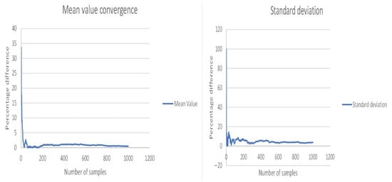
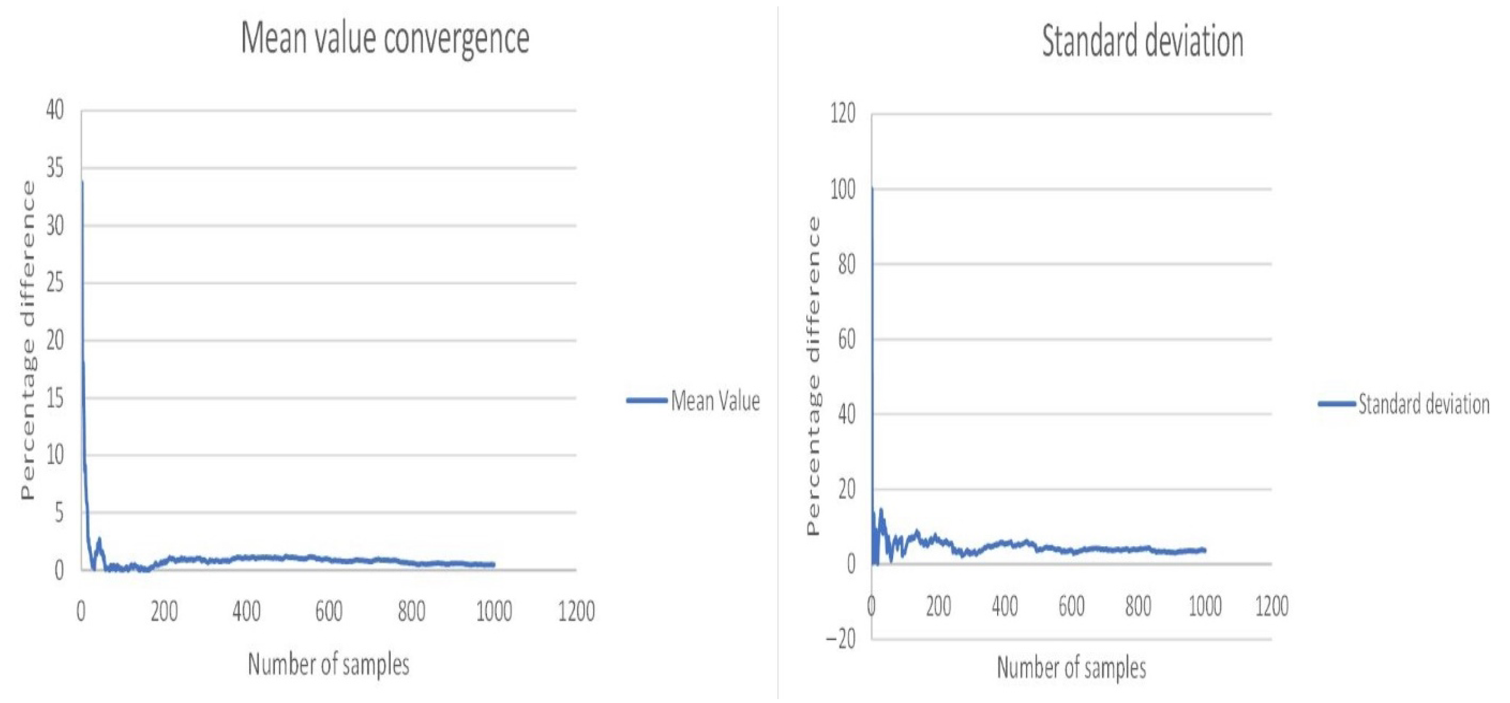
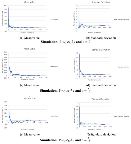
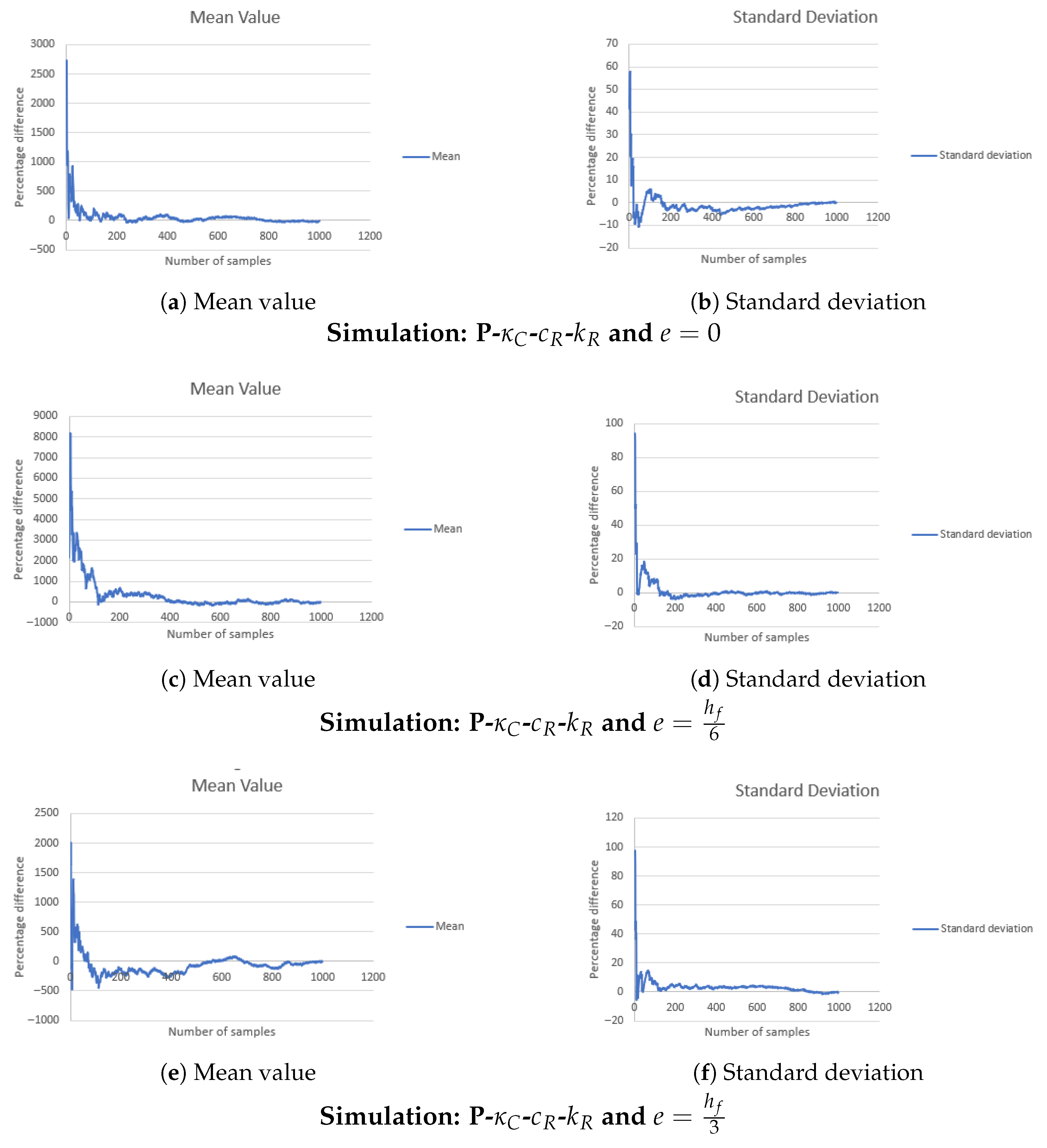
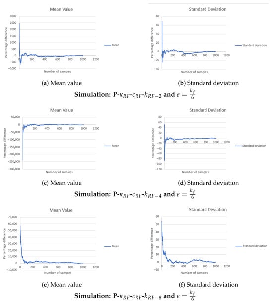
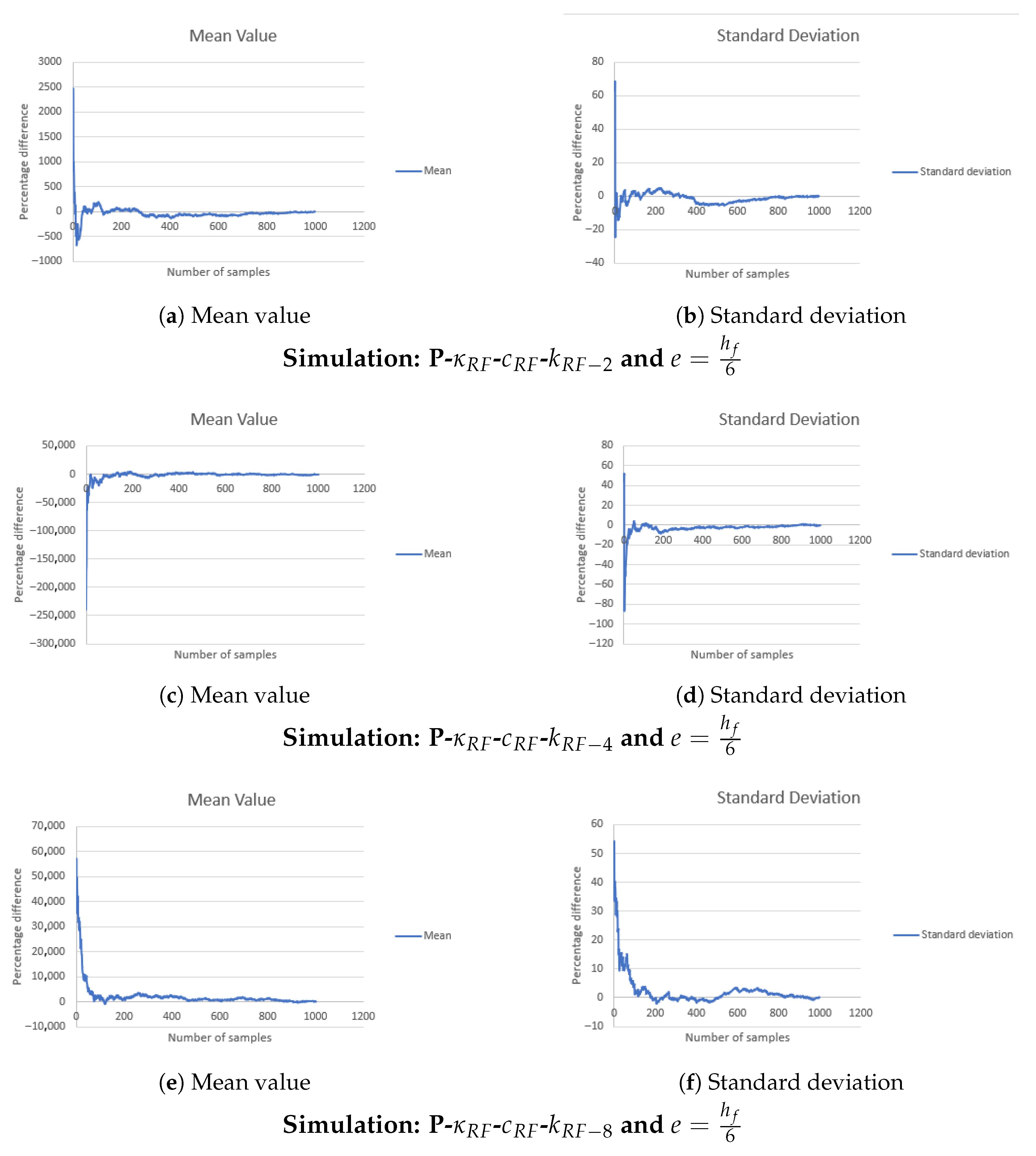
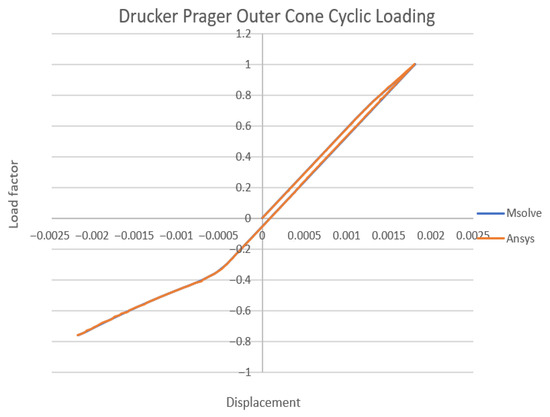
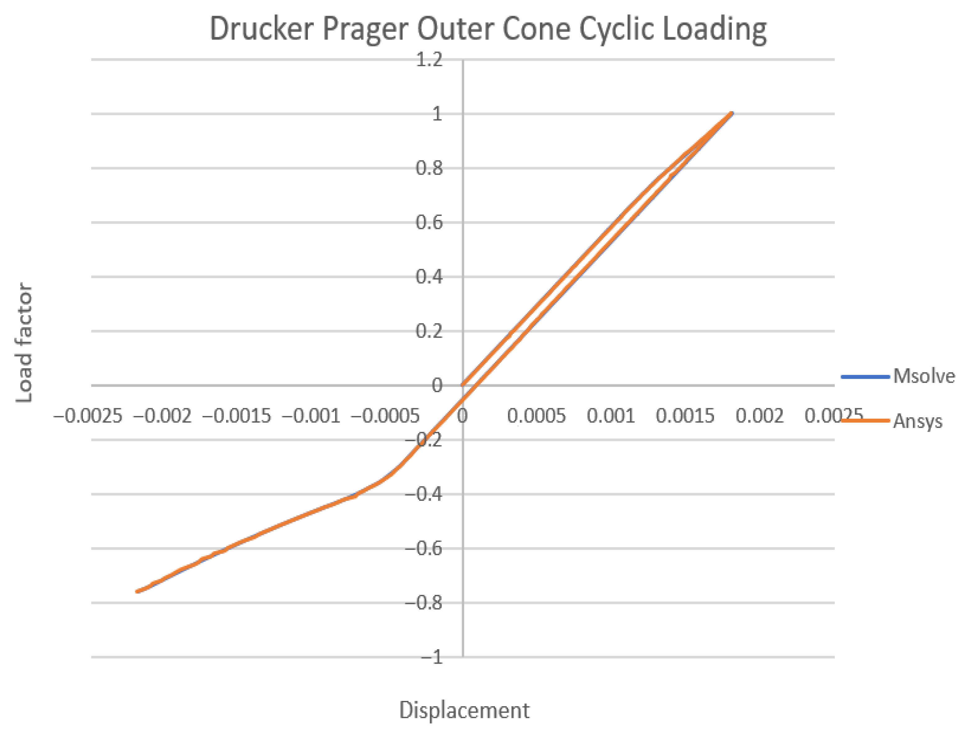
Static forces are applied and eight Fredholm eigenfunctions are used. The limit state is set as if the first Gaussian integration point represents the softening response (i.e., plastic hardening modulus H = 0, or else in this case, when the strain exceeds 0.001). All Monte Carlo analyses consist of 100 deterministic analyses, with input random vectors formulated with the aid of the Latin Hypercube Sampling methodology, which is shown to be enough to find the first two statistical moments of the output displacements, as explained in Figure 5. This holds for varying eccentricities and kinds of simulations, as depicted in Figure 6 and Figure 7. In all cases, the maximum relative deviation of the statistical moment is no more than 5%, and consequently, the 100 sampling size can be considered sufficient for determining the output statistics of this study. In terms of computational expense, a selected Monte Carlo analysis of this study was performed in about 36 h. If Monte Carlo simulations of 1000 random fair coin samplings were performed, the computational cost would be 400 h. Therefore, the proposed LHS framework requires approximately 9% of the computational time of standard Monte Carlo simulation. Analogous consideration can be made for the remaining simulations, not only in terms of computational cost, but also in terms of statistical convergence of average values and standard deviation. Cross-correlation in all material parameters is adopted as zero. The Drucker–Prager criterion is implemented with the outer-cone type of estimation in relation to the approximation using Mohr–Coulomb. Also the dilation is always the same as the friction angle. It should be mentioned here that the aforementioned analyses were performed with open source computational mechanics code MSolve (https://github.com/mgroupntua, accessed on 4 January 2026). For verification purposes, a deterministic test with Drucker–Prager and u–p formulation analysis was performed in comparison with ANSYS software 2025 R2 for cyclic loading. The displacement curves are portrayed in Figure 8. It is evident that the relative divergence is less than 3%; consequently, the code is providing reliable results for the deterministic response of the soil domain.
Figure 5.
Convergence of the mean value and the standard deviation of a randomly selected Monte Carlo simulation for the output failure load. The reference value of the percentage difference is the statistical moment in the 100 samples.
Figure 6.
Mean and standard deviation plots of convergence (part 1 of 2) for different stochastic analyses of this study for the output failure load. The reference value of the percentage difference is the statistical moment in the 100 samples.
Figure 7.
Mean and standard deviation plots of convergence (part 2 of 2) for different stochastic analyses of this study for the output failure load. The reference value of the percentage difference is the statistical moment in the 100 samples.
Figure 8.
Verification example of MSolve using Drucker–Prager constitutive model and u–p formulation. Comparison is made using ANSYS software.
5.2. Results Presentation
5.2.1. Limit Force and Respective Displacement Field
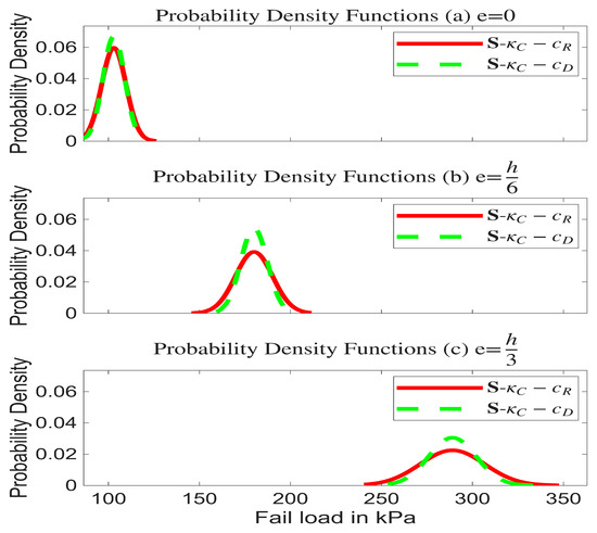
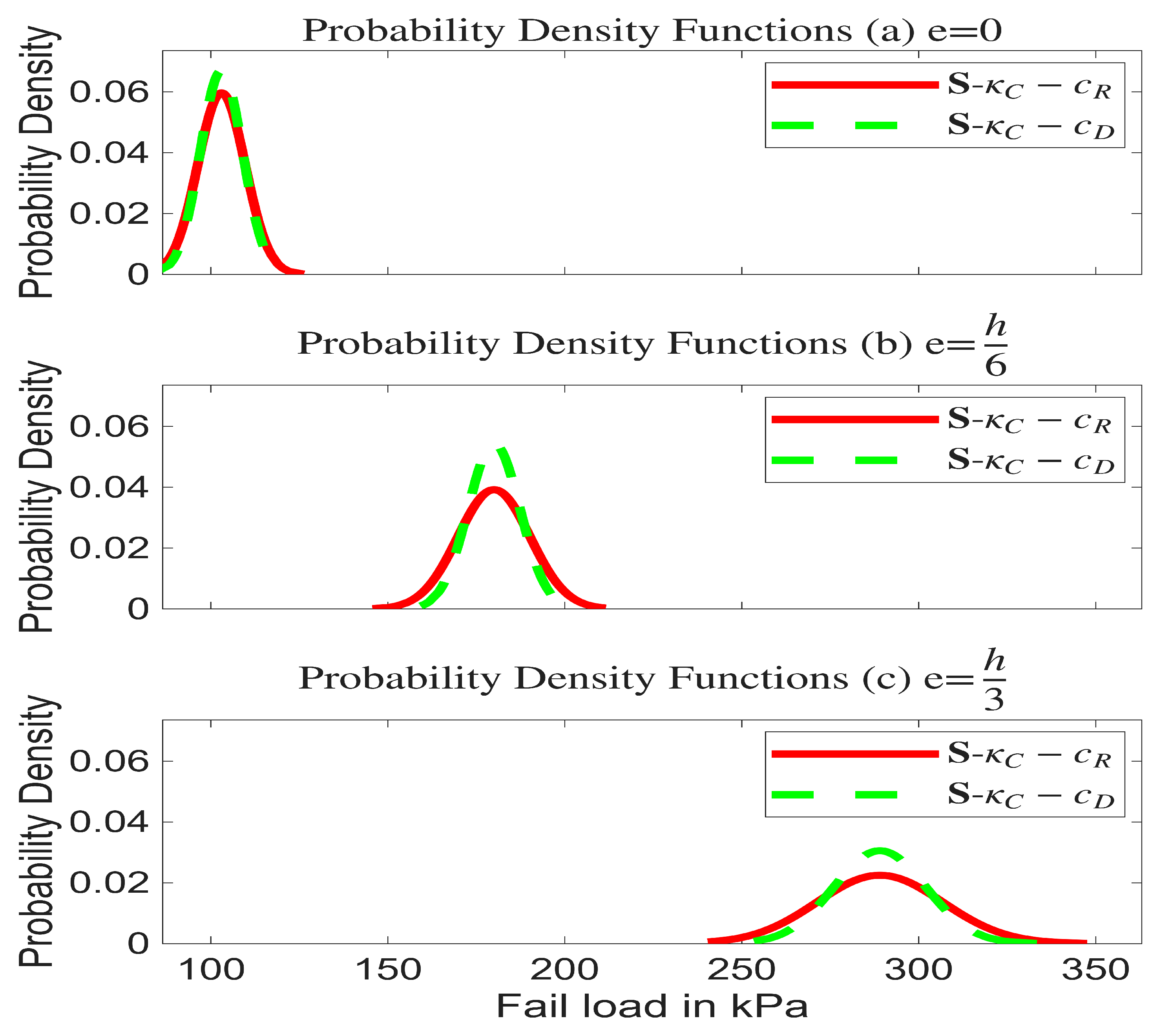
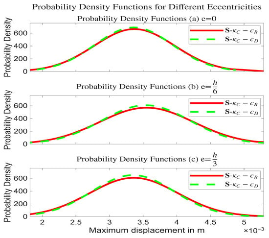
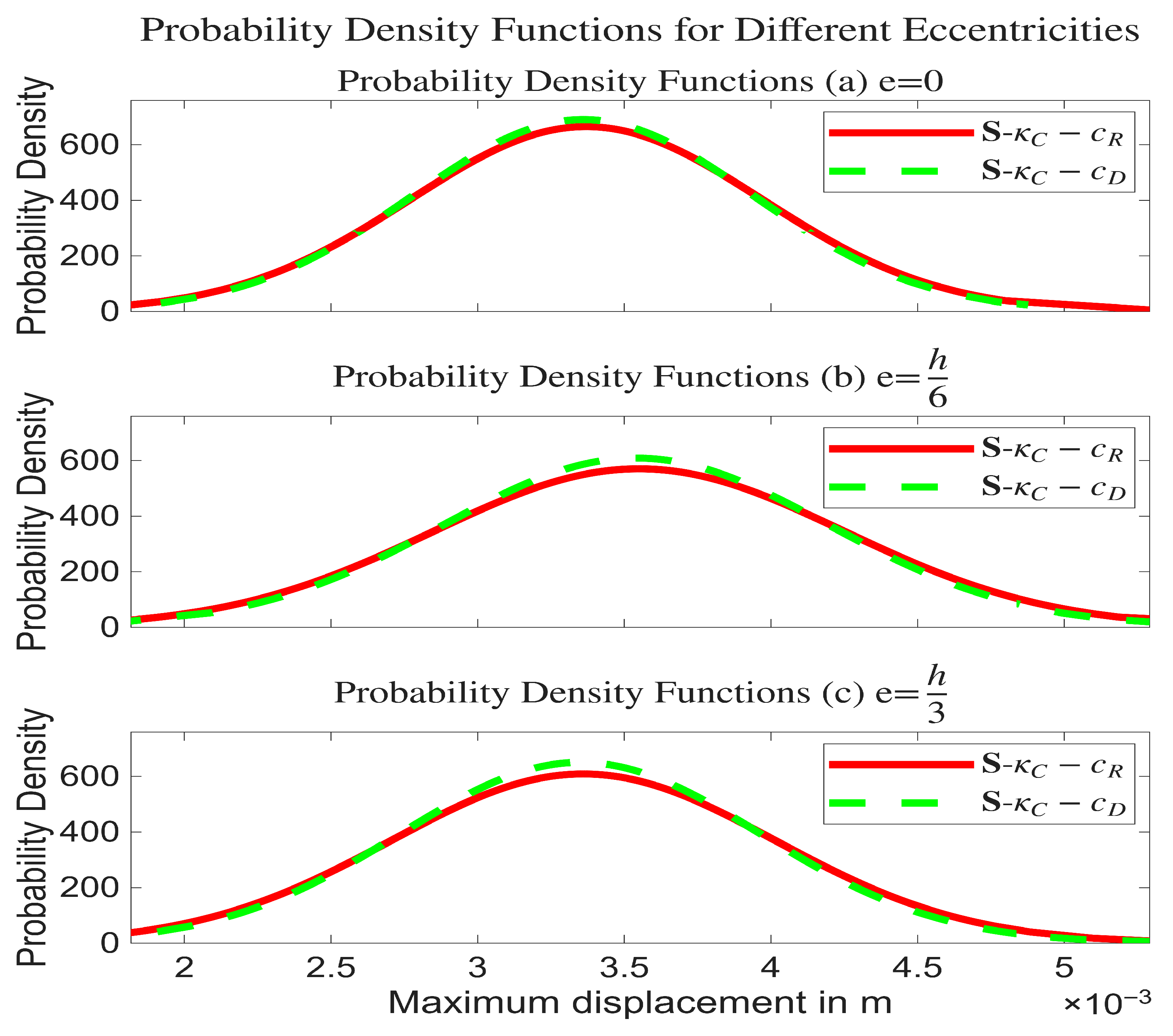
The statistical moments of the ultimate load, extreme displacements, and foundation rotation are presented in Figure 9, Figure 10, Figure 11, Figure 12, Figure 13, Figure 14, Figure 15 and Figure 16 and Table A1, which can be found in the Appendix A section. The mean values () of the footing settlement limit force, the minimum and the maximum displacement of the foundation, and the rotation of the foundation are portrayed in conjunction with the coefficient of variation (CoV) () and the minimum () and maximum () values attained from the stochastic analyses. It should be noted that the constant-with-depth representation of is emphasized, as this case exhibits the largest variability in all output parameters. This is also emphasized for the sake of clarity and simplicity. In Table 5, the summary of the main key findings of Table A1 are given.
Figure 9.
Output failure load probability density functions for dry non-porous soil continuum.
Figure 10.
Output failure maximum displacement probability density functions for dry non-porous soil continuum.
Figure 11.
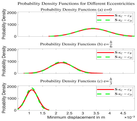
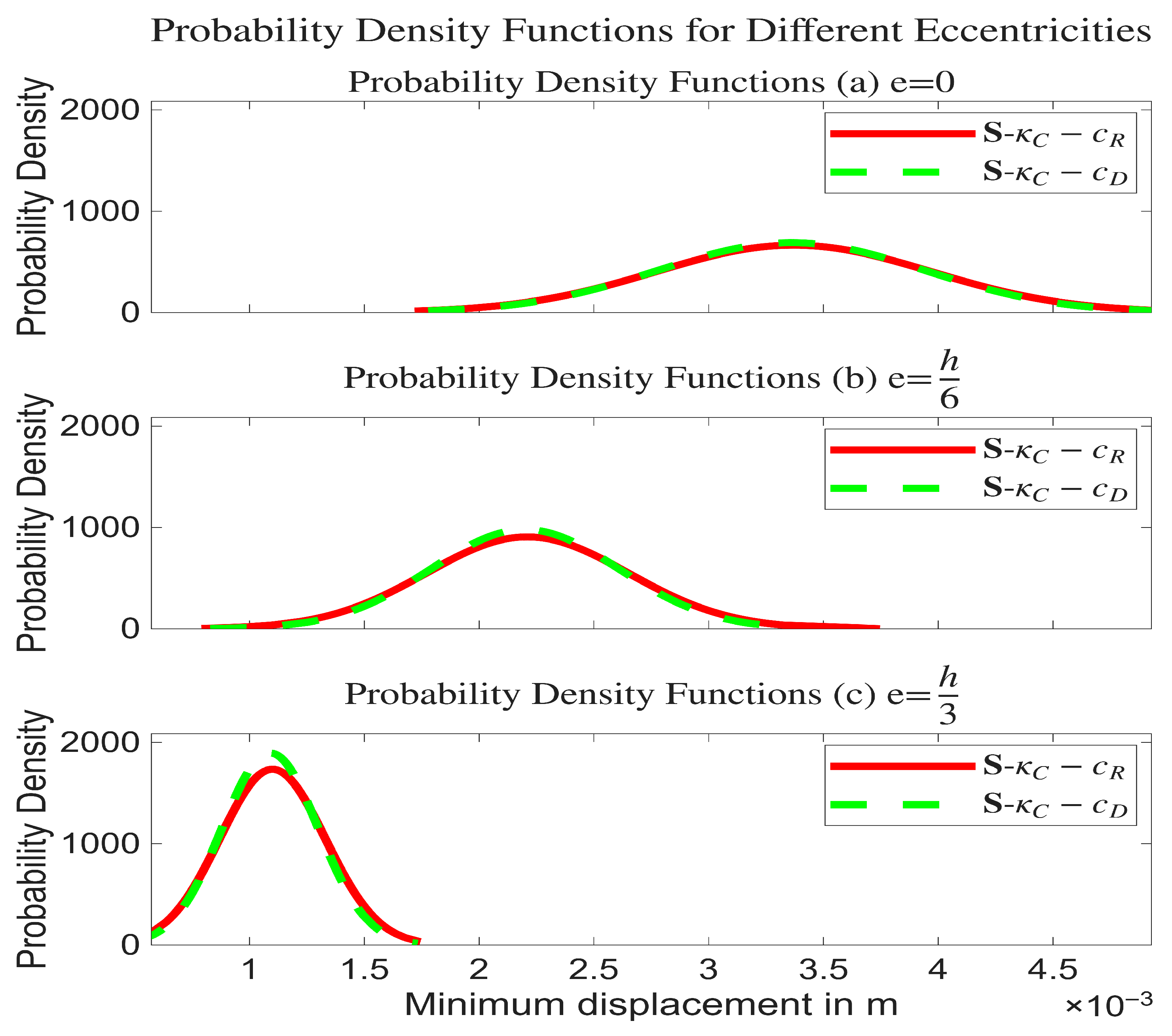
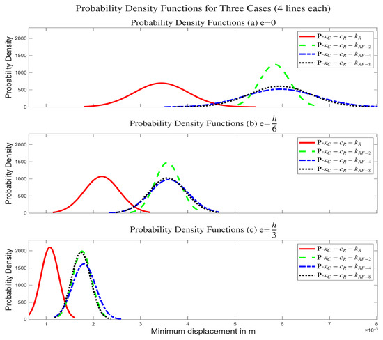
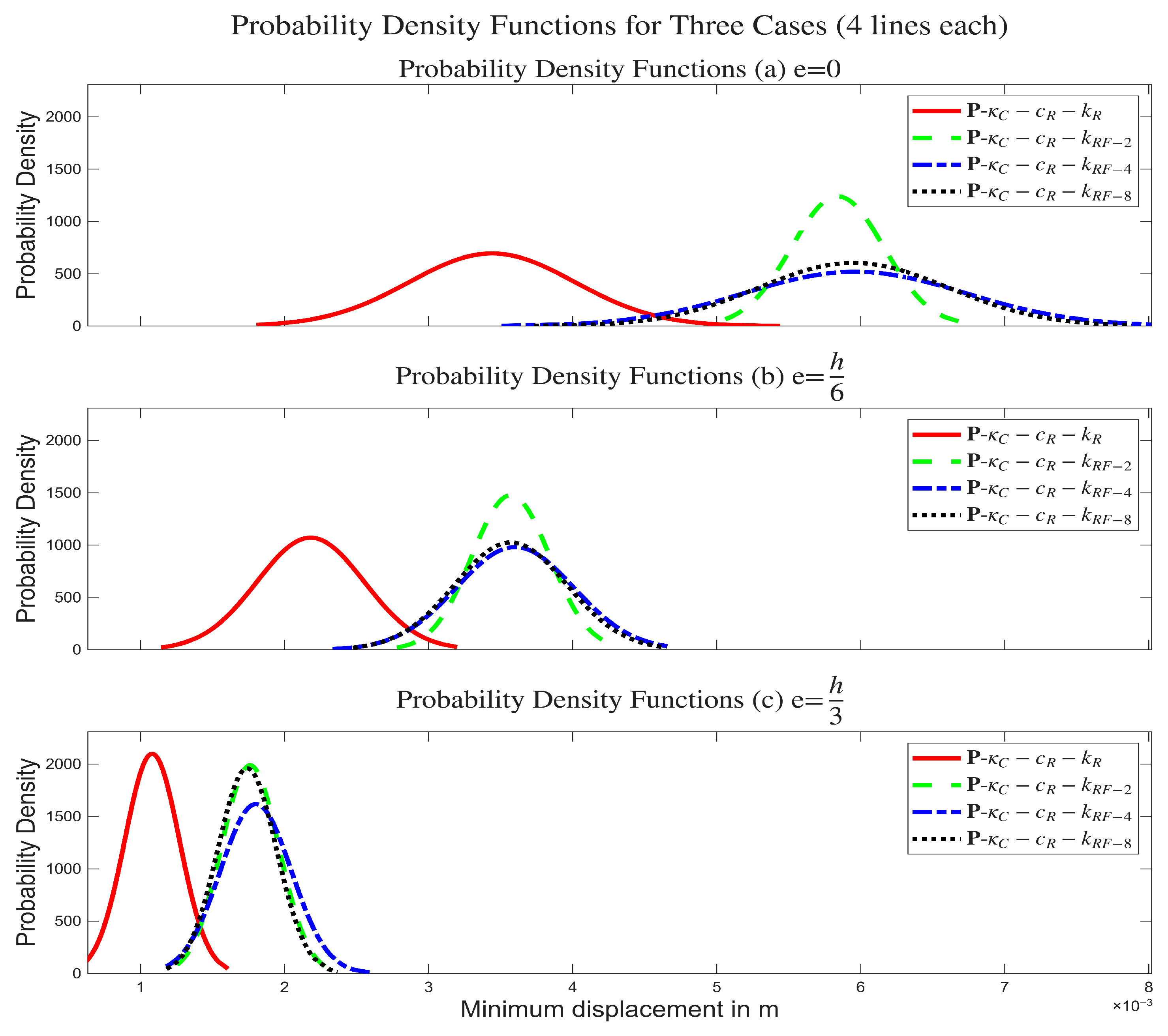
Output failure minimum displacement probability density functions for dry non-porous soil continuum.
Figure 12.
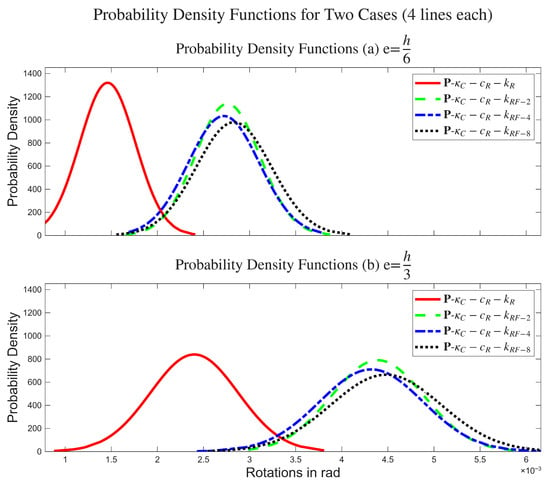
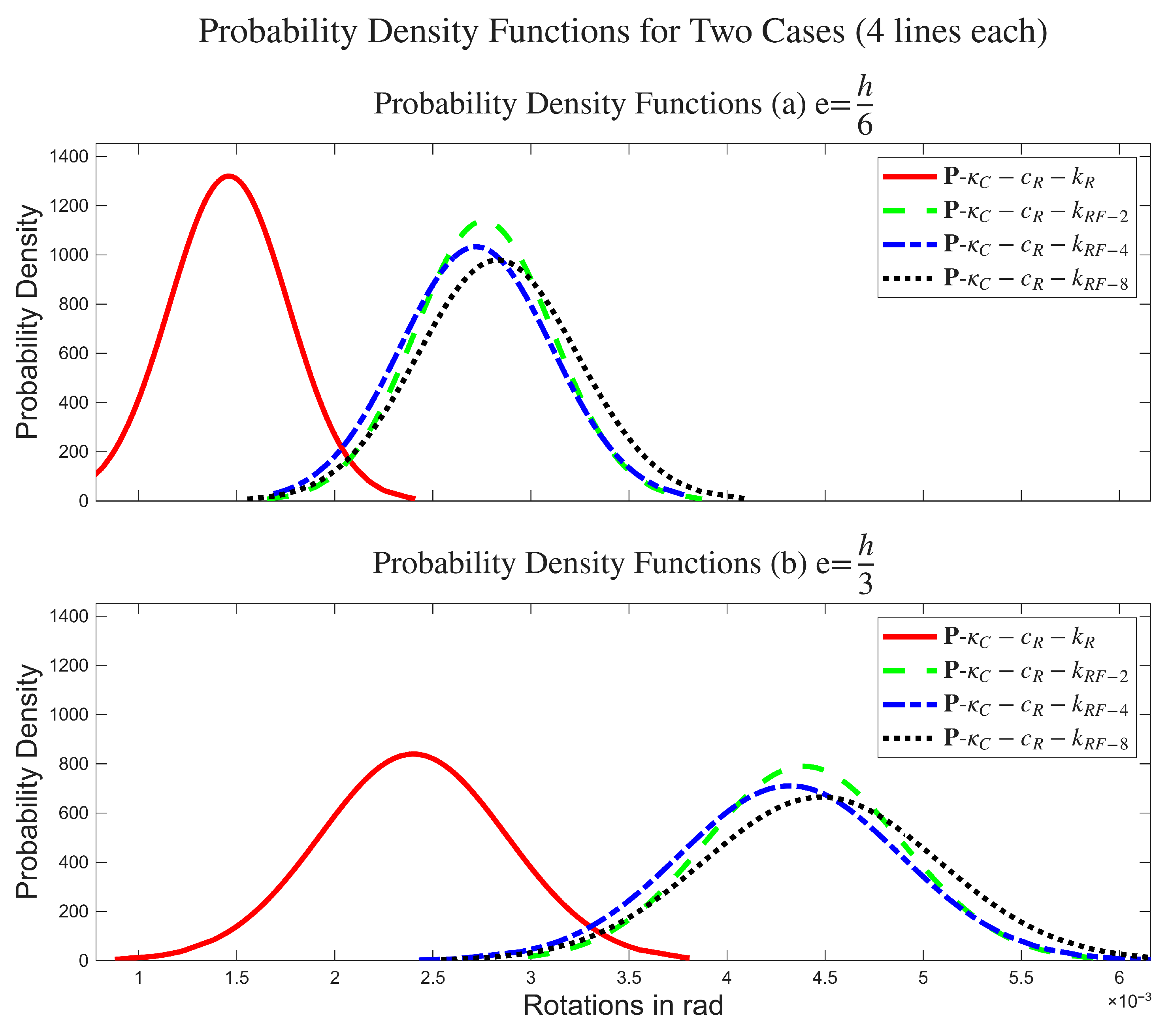
Output failure settlement rotation probability density functions for dry non-porous soil continuum.
Figure 13.
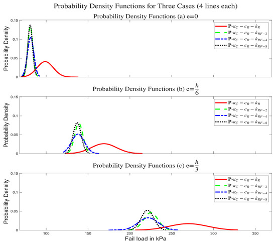
Output failure load probability density functions for wet porous soil continuum.
Figure 14.
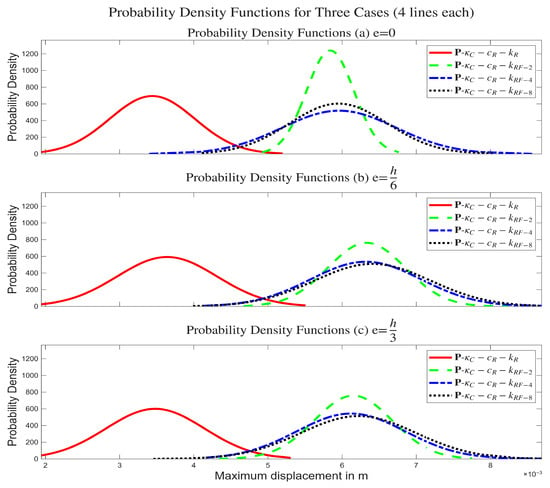
Output failure maximum displacement probability density functions for wet porous soil continuum.
Figure 15.
Output failure minimum displacement probability density functions for wet porous soil continuum.
Figure 16.
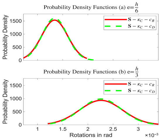
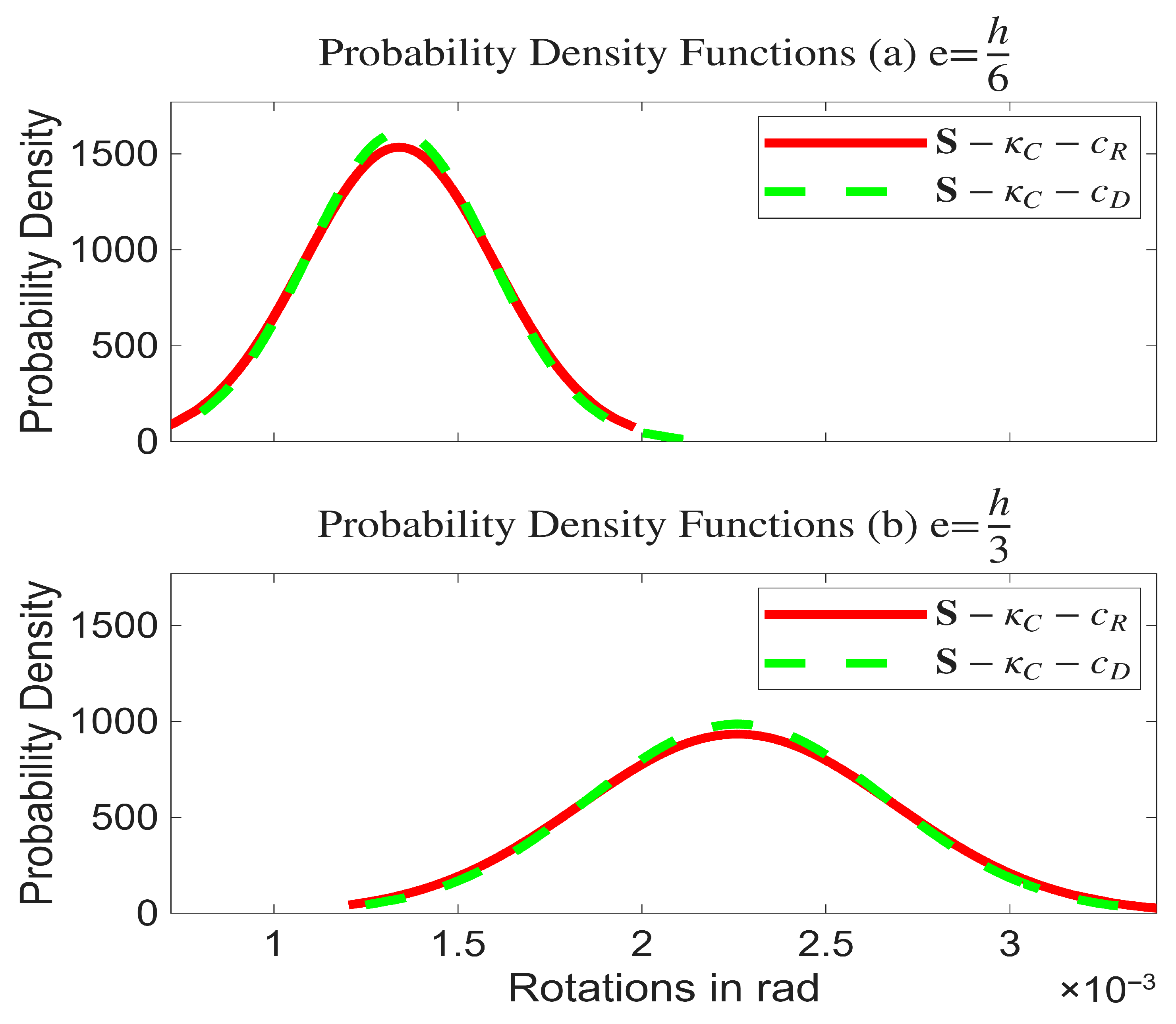
Output failure settlement rotation probability density functions for wet porous soil continuum.
Table 5.
Summary of the main key findings of Table A1.
As seen in Table A1, if dry soil continua are considered, larger mean limit-state displacements and smaller CoVs are evident if is adopted instead of . Larger mean limit-state loads and variability are evident if is adopted, for the majority of eccentricities analyzed. In the stochastic analyses of this study, the greatest CoV of the output for limit load is about 26% of the uncertainty of the input material parameters. The maximum CoV of the settlement displacement and rotations is about 80% of the value of 0.25 (referring to the minimum displacement CoV value in the -- simulation and ). The mean limit load for -- analysis and e = is 2.8 times larger than the corresponding value and e = 0, and the same applies for the corresponding values of the -- simulation. The greatest CoV of the fail force is located when no eccentricity is evident, while maximum and minimum displacements and rotations are having their maximum CoV when , , and , respectively. Subsequently, the most detrimental spatial representation of for the variability of all output parameters is the representation. The probability density functions of the dry non-porous simulations are given in Figure 9, Figure 10, Figure 11 and Figure 12. It can be seen that for limit forces, the mean value is augmented with the augmentation of the eccentricity. For maximum limit-state displacements, the augmentation of the eccentricity does not have a strictly monotonic effect on the mean value. However, for foundation minimum displacements and rotations, the augmentation of the eccentricity reduces the corresponding output value. The conclusions regarding the output displacements and the rotation of the settlement may be explained by the fact that if is adopted, the continuum layers of the upper area, being more compliant, present smaller variability of , resulting in smaller variability for strains and displacement fields. The soil continuum constant representation with respect to depth provides more homogeneous and increased stiffness; therefore, the Gauss points present greater stiffness, and greater limit loads are present.
The output variability of limit loads in wet porous analyses with deterministic shape functions has about the same influence of the eccentricity alteration compared to the dry solid analysis. The output uncertainty for displacement field and settlement rotation is more influence of the eccentricity change in comparison to the corresponding dry solid continua simulations, referring to Table A1. The greatest output CoV of limit force, located at -- for , is 40 % of the input variability. The corresponding greatest CoV of maximum settlement displacement is 0.76 times the uncertainty of the input parameters of 0.25 and is seen at -- for . As a result, if wet porous conditions are assumed, a decrease in the uncertainty of the limit loads is evident and in limit-state displacements, if a constant spatial representation for is assumed, a notable uncertainty augmentation is evident as portrayed in Figure 13, Figure 14, Figure 15 and Figure 16. Regarding the rotation of the shallow foundation if the constant representation of the unload path slope is adopted there exist a notable deviation related to the input variability. This is attained to the actuality that if constant stochastic representation of a material parameter is adopted, all Gauss integration points have greater variability resulting in larger CoV for displacement field and strains. The bulk modulus in porous poroelastic problems is related to the mean stress in wet porous problems and, in general, smaller than in dry non-porous analyses, it is evident that reduced mean values of limit forces and reduced uncertainty are anticipated, as a result of tensile limit state of the originated Gauss integration point. This is seen numerically in Appendix A in Table A2 and Table A3.
Wet porous simulations with all the material parameters represented by a random field are implemented as a generic methodology, because they consider the spatial representation of the uncertainty of the input soil properties. The greatest CoV of the output for limit load is 22% of the input variability, and analogous deductions hold for the largest settlement displacement. Regarding the rotation of the foundation, the output variability is about 57% of the input stochastic variation of 0.25, and is seen if the eccentricity is and b = 8 m. The mean values of limit load in wet porous stochastic process simulations are smaller (relative deviation up to 22%) compared to to the corresponding wet porous stochastic process simulations using deterministic shape relations for the material parameters, while the mean values for extreme limit-state displacements are larger compared to the corresponding simulations with linear representation for , about 1.74 times larger, as depicted in Table A1. In the case of wet porous stochastic process simulations, the augmentation of correlation length results in a non-strictly monotonic behavior for the CoV of the output limit loads, with b = 4 to represent the maximum output variability. Regarding the limit displacements in all eccentricities, as well as the rotation of the foundation, the extreme output variability is evident at b = 4 m. The most detrimental case corresponds to a reduction in the mean failure load; therefore, the critical spatial representation is identified as the one yielding the minimum mean value. Subsequently, the critical spatial representation for the mean value of ultimate force is the stochastic process simulations for all three material parameters. This is physically explained because the relative deviation of the material parameters is more than the respective analyses with deterministic interpolation functions. Subsequently, in the most compressible integration points, the variability is augmented; therefore, the total output variability is increased. The probability density functions of simulations are depicted in Figure 13, Figure 14, Figure 15 and Figure 16.
The results provide both qualitative and quantitative insights into the influence of input material parameter variability in wet porous limit-state simulations. The unload path slope randomness influences the mean values, and the variability of all output quantities. This effect in output CoV is profoundly evident if the representation of as a function of depth is constant. This is true also for the dry non-porous continuum, and it may be explained by being in a direct relation with bulk moduli, subsequently having a notable effect on the strain field, the displacement field, and the total stiffness of the soil continuum, resulting in a larger effect on the limit force.
The hydraulic variable of permeability k appears to have a smaller influence on limit-state loads and the corresponding settlement displacement field and rotation. The representation of the space of k appears to have a reduced effect of the output CoV in the majority of stochastic analyses for and c. Regarding a wet porous consolidation analysis with a certain force and deterministic details, the settlement displacements and limit-state stresses are not changed by the hydraulic permeability alteration because the pore pressure field is totally dissipated, as seen by the study results.
As a concluding remark, the uncertainty of critical state curve slope c of the constitutive law seems to have the most important influence on the uncertainty of the output for extreme shallow foundation loads if the constant representation and univariate random variable simulation are implemented. Larger mean values are attained if the case is used. Analogous considerations may be obtained regarding the displacement field and the rotations of the footing settlement. If a deterministic value for c is selected, the uncertainty of the output extreme loads is not notable; as a result, the influence of this material parameter is the most prominent compared to the others analyzed in this work. This is because c directly governs the limit state of a Gauss integration point, leading to a notable effect on the failure of the soil continuum.
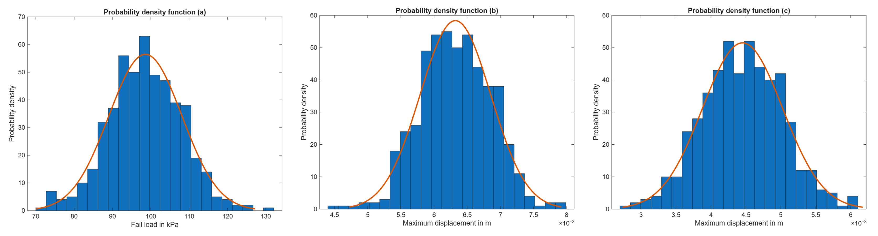
In order to demonstrate that the output parameters of this study follow the truncated normal or the lognormal univariate random variable, the histograms of three chosen stochastic analyses, with the corresponding probability density function fitting, are depicted in Figure 17. The empirical probability density functions predicted by the histograms may be simulated by the above-mentioned functions given in Equation (8) of Section 4. The extrema values given in Table A1 are reliable to set the truncation of the univariate normal distribution.
Figure 17.
Histograms of three randomly selected output Monte Carlo analyses: (a) Simulation -- for and limit-state force; (b) Simulation - for and maximum displacement; (c) Simulation - for and settlement rotation.
For providing a numerical justification of the stochastic nature of the outputs, the Kolmogorov–Smirnov test is implemented [59,60,61]. In the total of the set of output PDFs, the null hypothesis at the 5% significance level is shown to be accepted, as depicted in Table 6, whereas for the stochastic simulations presented in Figure 17, the above-mentioned test is performed. The extreme divergence in absolute terms of the empirical and theoretical cumulative distribution function (CDF) estimated by the stochastic analyses of Figure 17 is compared to the critical corresponding deviation in order to accept . It is evident that the critical value is larger than the extreme absolute deviation of the CDFs, and as a result, the random outputs follow a univariate Gaussian random variable. In addition, K–S test for Weibull distribution is performed for all Monte Carlo analyses. The tests did not accept the null hypothesis. Subsequently, the outputs are observed to follow a normal distribution, which could also be statistically founded based on the Central Limit Theorem. The physical and mechanics-oriented explanation for this behavior is the following: When nonlinear behavior is significant, especially near limit states, stresses and strains are inherently bounded. Subsequently, energy dissipation is maximized. This bounded nature limits extreme responses, which allows the system’s output probability density to approach a Gaussian distribution. The effect is further reinforced when many deterministic elements are aggregated. This is explained by the Central Limit Theorem; consequently, an approximately Gaussian system response is evident. This is in compliance with the existing scientific publications [62].
Table 6.
Kolmogorov–Smirnov test results for the stochastic analyses of Figure 17.
5.2.2. Limit-State Strain–Stress Field and Corresponding Curve
The statistical moments regarding the limit stress–strain relations and limit-state onset curve are given in Table A2 and Table A3, which are placed in the Appendix section. The variables presented are as follows: Mean values, CoVs, and minimum values for the volumetric stresses counterpart, denoted by ; and the deviatoric counterpart of the stresses, given as the Von Mises stresses, denoted by . Moreover, the mean value with the CoV of the volumetric strains counterpart, given by , and the deviatoric strains counterpart, denoted by , are given. Finally, the probability of onset Gauss integration point of the limit Meyerhoff curve for all stochastic analyses is portrayed. It is noted here that the volumetric strain at the limit state is tensile.
As portrayed in the dry non-porous simulations in Table A2, greater output uncertainty for limit stresses are attained if the case is adopted. However, the corresponding mean values are practically the same. Furthermore, for the case, there is greater variability of the limit strains in the majority of eccentricities, which are about 1.3‰ for the random variable case for c and about 1.35‰ for the deterministic distribution for critical state line inclination regarding the deviatoric counterpart. For the volumetric counterpart, the mean values are even smaller. Generally, from the stochastic analyses performed, it may be concluded that the percentage of plastic deviatoric strains is augmented, and subsequently, the distortional type of failure is critical. In all cases, the Gauss integration point (3.79, 2.21, 3.79) represents the most possible failure onset if eccentricity is greater than 0.
In wet porous simulations using deterministic shape relations for material parameters, greater uncertainty for volumetric and deviatoric stresses is attained at e = 0, , respectively, by using a deterministic value for c, and if the eccentricity is greater than zero, the representation is more detrimental. The permeability alteration significantly affects the variability of the output if the - is adopted for eccentricities , as demonstrated in Table A2. The greatest uncertainty of the output in limit volumetric and deviatoric state strains are both evident at e = for -- simulation. From the stochastic analyses performed, it can be seen that the deviatoric type of failure is most detrimental in all cases examined. As a concluding remark, as seen in Table A3, the most possible limit Gauss integration point onset is (2.21, 2.21, 2.79) for e = 0, (3.79, 2.21, 3.79) for e = , and (3.79, 2.21, 3.79) for e = , and this applies for all considerations that do not adopt stochastic processes for the input parameters.
In wet porous simulations with stochastic processes for material parameters, larger CoVs of the output for stresses are generally attained if b = 2 m, as depicted in Table A2. The deviatoric stresses possess the most detrimental correlation length b = 8 m, respectively, for e > 0. Regarding volumetric stresses, the critical correlation length for e = , , is, respectively, b = 2, 4 m. From the stochastic analyses performed, if the eccentricity exceeds zero, the distortional type of limit state is present. By referring to Table A3, the most possible limit-state onset is (2.21, 2.21, 2.79) for e = 0, and when e > 0, the most probable failure mechanism onset point is (3.79, 2.21, 3.79). In most cases, the probability of the most possible onset point is about 100 %. It should be mentioned here the importance of the Meyerhoff curve onset probability to the total probability of the full shape of the curve. The Meyerhoff curve is a function of the onset point position. Therefore, a probabilistic analysis of the onset point results to stochastic quantification of the full shape of the curve.
The comparison of the proposed framework results from the bearing capacity formulas from Terzaghi and Meyerhoff reveals the following. The Terzaghi value of bearing capacity for the mean value of a friction angle of 23 degrees is kN. The Meyerhoff value of bearing capacity for the mean value of a friction angle of 23 degrees is kN. In most cases, the Terzaghi estimation is greater than the mean estimation of this study; therefore, the Terzaghi prediction is on the safe side. In all cases the Meyerhoff estimation is smaller than the mean estimation of this study; therefore, the prediction of the present study is on the safe side. In Table 7, the summary of Terzaghi, Meyerhoff, and the present study estimations for failure load is given, considering that e = 0. The present study estimation has in parentheses the corresponding CoV. An indicative safety factor can be predicted by estimating the ratio of maximum to minimum value of fail loads of the Monte Carlo simulations implemented in this study. From the study conducted and Table A1, row for fail loads, a safety factor between 1.5 is sufficient to cover the uncertainty scenarios presented.
Table 7.
Comparison of the present study estimation with Terzaghi and Meyerhoff formulas for e = 0 and --- simulations. In parentheses is the CoV of the relevant simulation.
6. Conclusions
A computational study of the limit state of footing settlements in cohesionless soil continua is presented, employing wet porous finite element simulations with stochastic material parameters. This study objective is to offer a computational perspective to obtain reliable estimations about the limit stresses, loads, displacements, and rotations of the shallow foundation situated in cohesionless soil mass as a function of the input uncertainty. Additionally, the high fidelity finite element model, alongside an advanced constitutive model, is used. The numerical testing in this study comprises simulations of the stochastic finite element methodology via Monte Carlo analyses of a spatially uncertain cohesionless soil mass subjected to footing settlement force until the limit state is reached. The cohesionless soil is simulated through the Drucker–Prager model and the output random arrays of limit load, limit displacement, and the Gauss integration point, from which the failure curve onsets are attained. The study has the following limitations. Firstly, the stochastic fields could also be formulated using spectral representation. Moreover, different geometries of soil or foundation areas could be employed, such as soil slopes with adjacent foundations or cyclic-shaped foundations. Dynamic foundation loads may also be examined in order to investigate the dynamic failure of the soil. All of the aforementioned limitations demonstrate the future research that could be carried out to extend the present work.
The obtained output arrays indicate that extreme stresses, forces, displacements, and rotations follow a Gaussian univariate distribution, despite the pronounced material nonlinearity present at the limit state. The variability of material poroelasticity is important in the output variability for limit stresses, forces, and failure displacements, particularly if a constant representation with respect to the depth of the soil continuum is assumed. The same applies for the critical state curve derivative c. If a constant representation for is assumed, the CoV of the output extreme displacement is between 0.76 and 1.22 of the input variability. The hydraulic parameter of permeability affects the output uncertainty to a smaller degree. In wet porous material simulations, the limit force is smaller in comparison to the corresponding dry, solid material analyses. In practice, engineers should quantify the reload path slope as accurately as possible, in order to alleviate the uncertainty of the soil response. Furthermore, a possible prestress procedure would increase soil stiffness and strength and would also alleviate the variability of the soil’s predicted displacements once experimentally investigated. Finally, regarding the friction angle, the best experimental procedure of triaxial loading would result in more accurate failure load predictions. Regarding permeability, the exact determination through laboratory or in situ testing would contribute to uncertainty reduction to a smaller extent.
The stochastic processes for the material parameters result in the greatest mean limit strains, especially if the correlation length is smaller. The greater uncertainty for limit stresses in both volumetric and deviatoric counterparts is evident when the critical state line inclination is not deterministic. In wet porous stochastic processes simulations for all investigated eccentricities, the distortional type of failure is critical. When deterministic spatial representations of the material parameters are assumed, the deviatoric failure mode is identified as the most detrimental. The volumetric strains at failure are far smaller than the respective deviatoric ones. The deviatoric strains are in the limit values for linear equivalent analyses. In conclusion, in the majority of cases, (3.79, 2.21, 3.79) is the most detrimental Gauss integration point limit-state onset, and may be assumed as the originating place of the Meyerhoff curve.
Funding
This research received no external funding.
Institutional Review Board Statement
Not applicable.
Informed Consent Statement
Not applicable.
Data Availability Statement
The raw data supporting the conclusions of this article will be made available by the author on request.
Acknowledgments
The author acknowledges Emeritus Manolis Papadrakakis for his constant academic enlightenment.
Conflicts of Interest
The author declares no conflicts of interest.
Appendix A
The following Tables are placed in this section. All reported numerical values are rounded to a level consistent with the uncertainty of the input parameters.
References
- Terzaghi, K.V. Theoretical Soil Mechanics; Wiley and Sons: Hoboken, NJ, USA, 1966. [Google Scholar]
- Zhou, H.; Zheng, G.; Yin, X.; Jia, R.; Yang, X. The bearing capacity and failure mechanism of a vertically loaded strip footing placed on the top of slopes. Comput. Geotech. 2018, 94, 12–21. [Google Scholar] [CrossRef] [Scilit]
- Naderi, E.; Asakereh, A.; Dehghani, M. Bearing Capacity of Strip Footing on Clay Slope Reinforced with Stone Columns. Arab. J. Sci. Eng. 2018, 43, 5559–5572. [Google Scholar] [CrossRef] [Scilit]
- Sultana, P.; Dey, A.K. Estimation of Ultimate Bearing Capacity of Footings on Soft Clay from Plate Load Test Data Considering Variability. Indian Geotech. J. 2019, 49, 170–183. [Google Scholar] [CrossRef] [Scilit]
- Fu, D.; Zhang, Y.; Yan, Y. Bearing capacity of a side-rounded suction caisson foundation under general loading in clay. Comput. Geotech. 2020, 123, 103543. [Google Scholar] [CrossRef] [Scilit]
- Li, S.; Yu, J.; Huang, M.; Leung, G. Upper bound analysis of rectangular surface footings on clay with linearly increasing strength. Comput. Geotech. 2021, 129, 103896. [Google Scholar] [CrossRef] [Scilit]
- Rao, P.; Liu, Y.; Cui, J. Bearing capacity of strip footings on two-layered clay under combined loading. Comput. Geotech. 2015, 69, 210–218. [Google Scholar] [CrossRef] [Scilit]
- Papadopoulou, K.; Gazetas, G. Shape Effects on Bearing Capacity of Footings on Two-Layered Clay. Geotech. Geol. Eng. 2020, 38, 1347–1370. [Google Scholar] [CrossRef] [Scilit]
- Michalowski, R.L. An Estimate of the Influence of Soil Weight on Bearing Capacity Using Limit Analysis. Soils Found. 1997, 37, 57–64. [Google Scholar] [CrossRef] [Scilit] [PubMed]
- Michalowski, R.L. Upper-bound load estimates on square and rectangular footings. Geotechnique 2001, 51, 787–798. [Google Scholar] [CrossRef]
- Martin, C. Exact bearing capacity calculations using the method of characteristics. In Proceedings of the 11th International Conference IACMAG, Graz, Austria, 19–24 June 2005. [Google Scholar]
- Matthies, H.G.; Brenner, C.E.; Butcher, G.; Soares, C.G. Uncertainties in probabilistic numerical analysis of structures and solids- Stochastic finite elements. Struct. Saf. 1997, 19, 283–336. [Google Scholar] [CrossRef] [Scilit]
- Assimaki, D.; Pecker, A.; Popescu, R.; Prevost, J. Effects of spatial variabilty of soil properties on surface ground motion. J. Earthq. Eng. 2003, 7, 1–44. [Google Scholar] [CrossRef] [Scilit]
- Popescu, R.; Deodatis, G.; Nobahar, A. Effects of random heterogeneity of soil properties on bearing capacity. Probabilistic Eng. Mech. 2005, 20, 324–341. [Google Scholar] [CrossRef] [Scilit]
- Meftah, F.; Dal-Pont, S.; Schrefler, B.A. A three-dimensional staggered finite element approach for random parametric modeling of thermo-hygral coupled phenomena in porous media. Int. J. Numer. Anal. Methods Geomech. 2012, 36, 574–596. [Google Scholar] [CrossRef] [Scilit]
- Li, D.Q.; Qi, X.H.; Cao, Z.J.; Tang, X.S.; Zhou, W.; Phoon, K.K.; Zhou, C.B. Reliability analysis of strip footing considering spatially variable undrained shear strength that linearly increases with depth. Soils Found. 2015, 55, 866–880. [Google Scholar] [CrossRef] [Scilit]
- Wang, T.; Chen, W.; Li, T.; Connolly, D.P.; Luo, Q.; Liu, K.; Zhang, W. Surrogate-assisted uncertainty modeling of embankment settlement. Comput. Geotech. 2023, 159, 105498. [Google Scholar] [CrossRef] [Scilit]
- Kumar, V.; Burman, A.; Portelinha, F.H.M.; Kumar, M.; Das, G. Influence of Variation of Soil Properties in Bearing Capacity and Settlement Analysis of a Strip Footing Using Random Finite Element Method. Civ. Eng. Infrastructures J. 2024, 57, 383–403. [Google Scholar] [CrossRef]
- Karhunen, K. Uber lineare Methoden in der Wahrscheinlichkeitsrechnung. In Annales Academiae Scientarium Fenniciae; Series A.1; Suomalainen Tiedeakatemia: Helsinki, Finland, 1947; Volume 37, pp. 1–79. [Google Scholar]
- Ghanem, R.; Spanos, D. Stochastic Finite Elements: A Spectral Approach; Springer: Berlin/Heidelberg, Germany, 1991; Volume 1, pp. 1–214. [Google Scholar] [CrossRef] [Scilit]
- Papadrakakis, M.; Papadopoulos, V. Robust and efficient methods for the stochastic finite element analysis using Monte Carlo simulation. Comput. Methods Appl. Mech. Eng. 1996, 134, 325–340. [Google Scholar] [CrossRef] [Scilit]
- Sett, K.; Jeremic, B. Probabilistic elasto-plasticity: Solution and verification in 1D. Acta Geotech. 2007, 2, 211–220. [Google Scholar] [CrossRef] [Scilit]
- Liu, W.; Sun, Q.; Miao, H.; Li, J. Nonlinear stochastic seismic analysis of buried pipeline systems. Soil Dyn. Earthq. Eng. 2015, 74, 69–78. [Google Scholar] [CrossRef] [Scilit]
- Ali, A.; Lyamin, A.; Huang, J.; Li, J.; Cassidy, M.; Sloan, S. Probabilistic stability assessment using adaptive limit analysis and random fields. Acta Geotech. 2017, 12, 937–948. [Google Scholar] [CrossRef] [Scilit]
- Brantson, E.T.; Ju, B.; Wu, D.; Gyan, P.S. Stochastic porous media modeling and high-resolution schemes for numerical simulation of subsurface immiscible fluid flow transport. Acta Geophys. 2018, 66, 243–266. [Google Scholar] [CrossRef] [Scilit]
- Chwała, M. Undrained bearing capacity of spatially random soil for rectangular footings. Soils Found. 2019, 59, 1508–1521. [Google Scholar] [CrossRef] [Scilit]
- Shi, J.K.; Zhang, J.Z.; Zhao, S.; Guan, Z.C.; Huang, H.W. Probabilistic analysis of ground surface settlement induced by super large diameter shield tunneling based on 3D random finite element method. Comput. Geotech. 2025, 181, 107111. [Google Scholar] [CrossRef] [Scilit]
- Zhou, X.; Wang, T. Uncertainty Analysis and Risk Assessment for Variable Settlement Properties of Building Foundation Soils. Buildings 2025, 15, 2369. [Google Scholar] [CrossRef] [Scilit]
- Olsson, A.; Sandberg, G.; Dahlblom, O. On Latin hypercube sampling for structural reliability analysis. Struct. Saf. 2003, 25, 47–68. [Google Scholar] [CrossRef] [Scilit]
- Simoes, J.; Neves, L.; Antao, A.; Guerra, N. Reliability assessment of shallow foundations on undrained soils considering soil spatial variability. Comput. Geotech. 2020, 119, 103369. [Google Scholar] [CrossRef] [Scilit]
- da Fonseca, J.P.; Potts, D.M. Nonlinear response of drained clay to footings. Comput. Struct. 1978, 8, 123–134. [Google Scholar] [CrossRef] [Scilit]
- Hsieh, C.W.; Wang, M.C. Bearing Capacity Determination Method for Strip Surface Footings Underlain by Voids. Transp. Res. Rec. 1991, 1336, 1–12. [Google Scholar]
- Keba, E.; Isobe, K. Bearing Capacity of a Shallow Foundation Above Soil with a Cavity Based on Rigid Plastic FEM. Appl. Sci. 2024, 14, 1975. [Google Scholar] [CrossRef] [Scilit]
- Feng, D.; Gan, L.; Xiong, M.; Li, W.; Huang, Y. Uncertainty analysis of 3D post-failure behavior in landslide and reinforced slope based on the SPH method and the random field theory. Eng. Geol. 2025, 350, 108017. [Google Scholar] [CrossRef] [Scilit]
- Stavroulakis, G.; Giovanis, D.; Papadopoulos, V.; Papadrakakis, M. A GPU domain decomposition solution for spectral stochastic finite element method. Comput. Methods Appl. Mech. Eng. 2014, 327, 392–410. [Google Scholar] [CrossRef] [Scilit]
- Stavroulakis, G.; Giovanis, D.; Papadopoulos, V.; Papadrakakis, M. A new perspective on the solution of uncertainty quantification and reliability analysis of large-scale problems. Comput. Methods Appl. Mech. Eng. 2014, 276, 627–658. [Google Scholar] [CrossRef] [Scilit]
- Savvides, A.; Papadrakakis, M. A computational study on the uncertainty quantification of failure of clays with a modified Cam-Clay yield criterion. SN Appl. Sci. 2021, 3, 659. [Google Scholar] [CrossRef] [Scilit]
- Savvides, A.; Papadrakakis, M. Uncertainty Quantification of Failure of Shallow Foundation on Clayey Soils with a Modified Cam-Clay Yield Criterion and Stochastic FEM. Geotechnics 2022, 2, 348–384. [Google Scholar] [CrossRef] [Scilit]
- Robert, C.P. Simulation of truncated normal variables. Stat. Comput. 1995, 5, 121–125. [Google Scholar] [CrossRef] [Scilit]
- Barr, D.R.; Sherrill, E.T. Mean and variance of truncated normal distributions. Am. Stat. 1999, 53, 357–361. [Google Scholar] [CrossRef] [Scilit]
- Teshager, D.K.; Chwała, M.; Puła, W. Probabilistic analysis of foundation settlement considering spatial variability in soil parameters: A comparison of hardening soil model and Mohr-Coulomb. In Georisk: Assessment and Management of Risk for Engineered Systems and Geohazards; Taylor & Francis Ltd.: Oxfordshire, UK, 2025; pp. 1–21. [Google Scholar] [CrossRef] [Scilit]
- Melenk, J.M.; Babuska, I. The partition of unity finite element method: Basic theory and applications. Comput. Methods Appl. Mech. Eng. 1996, 139, 289–314. [Google Scholar] [CrossRef] [Scilit]
- Szabo, B.; Babuska, I. Intoduction to finite element analysis. Formulation, verification and validation. Wiley Ser. Comput. Mech. 2011, 1, 1–382. [Google Scholar] [CrossRef] [Scilit]
- Bowles, J.E. Foundation Analysis and Design, 7th ed.; McGraw-Hill Education: New York, NY, USA, 2012. [Google Scholar]
- Lambe, T.W.; Whitman, R.V. Soil Mechanics; John Wiley & Sons: New York, NY, USA, 1969. [Google Scholar]
- Wu, Y.; Zhou, X.; Gao, Y.; Zhang, L.; Yang, J. Effect of soil variability on bearing capacity accounting for non-stationary characteristics of undrained shear strength. Comput. Geotech. 2019, 110, 199–210. [Google Scholar] [CrossRef] [Scilit]
- Almhaidib, A.I. Compressibility of Soil (CE 481 Lecture Notes, Chapter 11). Department of Civil Engineering, King Saud University, n.d. Available online: https://faculty.ksu.edu.sa/sites/default/files/CE%20481%20Compressibility%20of%20Soil%20%282%29.pdf (accessed on 4 January 2026).
- Yue, Q. Stochastic settlement simulation of soil deposit using a new efficient spatial correlation model. In Proceedings of the 7th International Symposium on Geotechnical Safety and Risk (ISGSR), Taipei, Taiwan, 11–13 December 2019; Ching, J., Li, D., Zhang, J., Eds.; Research Publishing: Singapore, 2019; pp. 213–221. [Google Scholar]
- Alibeikloo, M.; Khabbaz, H.; Fatahi, B. Random field reliability analysis for time-dependent behaviour of soft soils considering spatial variability of elastic visco-plastic parameters. Reliab. Eng. Syst. Saf. 2022, 219, 108254. [Google Scholar] [CrossRef] [Scilit]
- Schofield, A.N.; Wroth, C.P. Critical State Soil Mechanics; McGraw-Hill: New York, NY, USA, 1968. [Google Scholar]
- Original Cam-Clay Model. Engineering LibreTexts, n.d. Granular Materials Section, TLP Library I. Available online: https://eng.libretexts.org/Bookshelves/Materials_Science/TLP_Library_I/33%3A_Granular_Materials/33.7%3A_Original_Cam-Clay_Model (accessed on 4 January 2026).
- Yu, H.S.; Zhang, G.; Wang, L. A unified critical state model for geomaterials with an application to tunnelling. J. Rock Mech. Geotech. Eng. 2019, 11, 464–480. [Google Scholar] [CrossRef] [Scilit]
- Sun, J.; Guan, H.; Sun, B.; Wan, Y. Investigating the impact of random field element size on soil slope reliability analysis. Appl. Sci. 2024, 14, 9237. [Google Scholar] [CrossRef] [Scilit]
- Tran Vu-Hoang, T.; Nguyen, T.; Shiau, J.; Ly-Khuong, D.; Pham-Tran, H. Probabilistic analysis of active earth pressures in spatially variable soils using machine learning and confidence intervals. Sci. Rep. 2025, 15, 8823. [Google Scholar] [CrossRef] [Scilit]
- Xia, Y.; Li, N. High-resolution estimation of soil saturated hydraulic conductivity via upscaling and Karhunen–Loève expansion within DREAM(ZS). Appl. Sci. 2024, 14, 4521. [Google Scholar] [CrossRef] [Scilit]
- Lewis, R.W.; Schrefler, B.A. The Finite Element Method in the Deformation and Consolidation of Porous Media; Wiley Sons: Hoboken, NJ, USA, 1988; Volume 1, pp. 1–508. [Google Scholar] [CrossRef] [Scilit]
- Zienkiewicz, O.C.; Chan, A.H.C.; Pastor, M.; Schrefler, B.A.; Shiomi, T. Computational Geomechanics with Special Reference to Earthquake Engineering; Wiley: Chichester, UK, 1999; Volume 1, pp. 17–49. [Google Scholar]
- Stickle, M.M.; Yague, A.; Pastor, M. Free Finite Element Approach for Saturated Porous Media: Consolidation. Math. Probl. Eng. 2016, 2016, 4256079. [Google Scholar] [CrossRef] [Scilit]
- Kolmogorov, A. Sulla determinazione empirica di una legge di distribuzione. G. Ist. Ital. Attuari 1933, 4, 83–91. [Google Scholar]
- Smirnov, N. Table for estimating the goodness of fit of empirical distributions. Ann. Math. Stat. 1948, 19, 279–281. [Google Scholar] [CrossRef] [Scilit]
- Dimitrova, D.; Kaishev, V.; Tan, S. Computing the Kolmogorov-Smirnov Distribution when the Underlying cdf is Purely Discrete, Mixed or Continuous. J. Stat. Softw. 2019, 95, 1–42. [Google Scholar] [CrossRef] [Scilit]
- Fenton, G.; Griffiths, D. Bearing Capacity Prediction of Spatially Random c-ϕ Soils. Can. Geotech. J. 2003, 40, 54–65. [Google Scholar] [CrossRef] [Scilit]

Disclaimer/Publisher’s Note: The statements, opinions and data contained in all publications are solely those of the individual author(s) and contributor(s) and not of MDPI and/or the editor(s). MDPI and/or the editor(s) disclaim responsibility for any injury to people or property resulting from any ideas, methods, instructions or products referred to in the content. |
© 2026 by the author. Licensee MDPI, Basel, Switzerland. This article is an open access article distributed under the terms and conditions of the Creative Commons Attribution (CC BY) license.