
Fully Polarimetric L-Band Synthetic Aperture Radar for the Estimation of Tree Girth as a Representative of Stand Productivity in Rubber Plantations


Abstract
:
1. Introduction
2. Materials and Methods
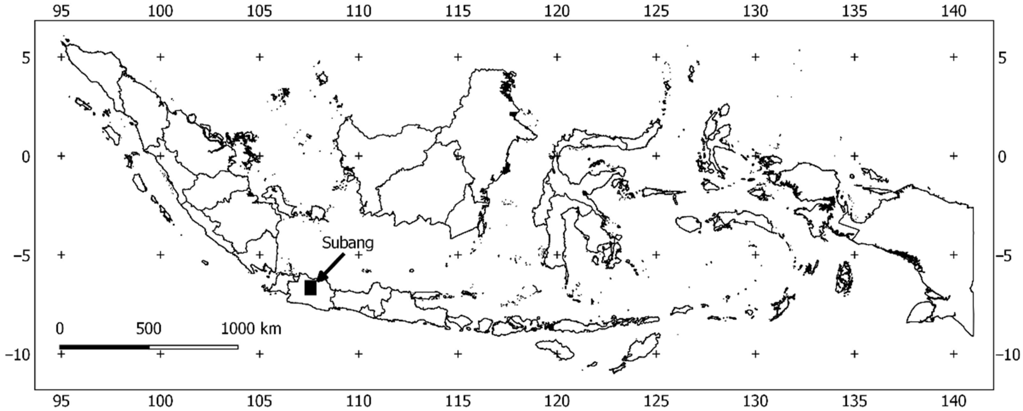
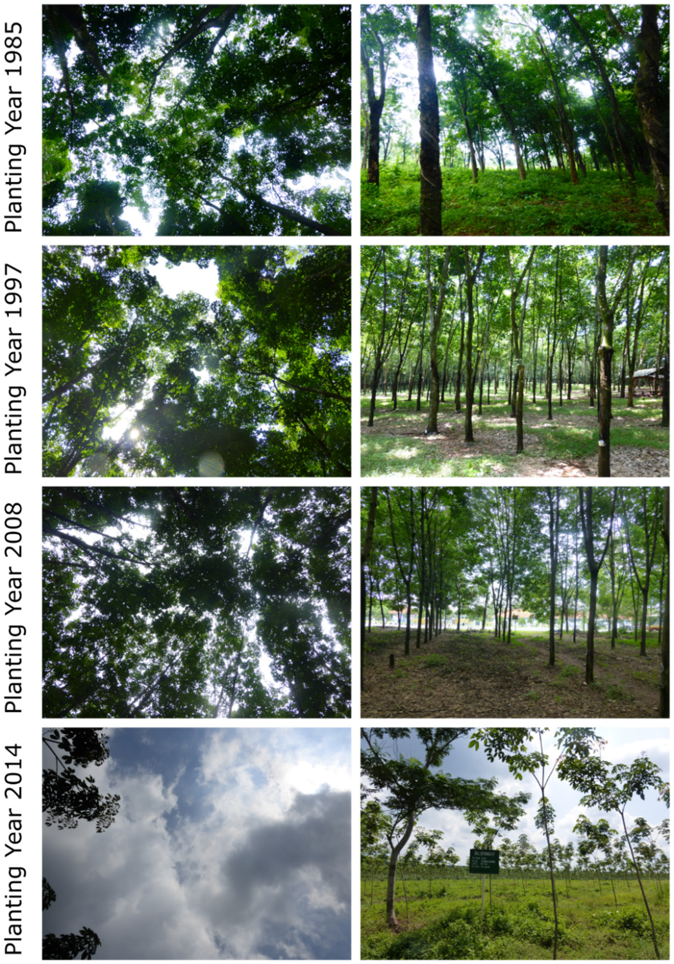
2.1. Test Site
2.2. Datasets and Analysis
3. Results
3.1. Performance of Backscatter Coefficients
3.2. Accuracy Analysis of Decomposition Features
3.3. Feature Stack
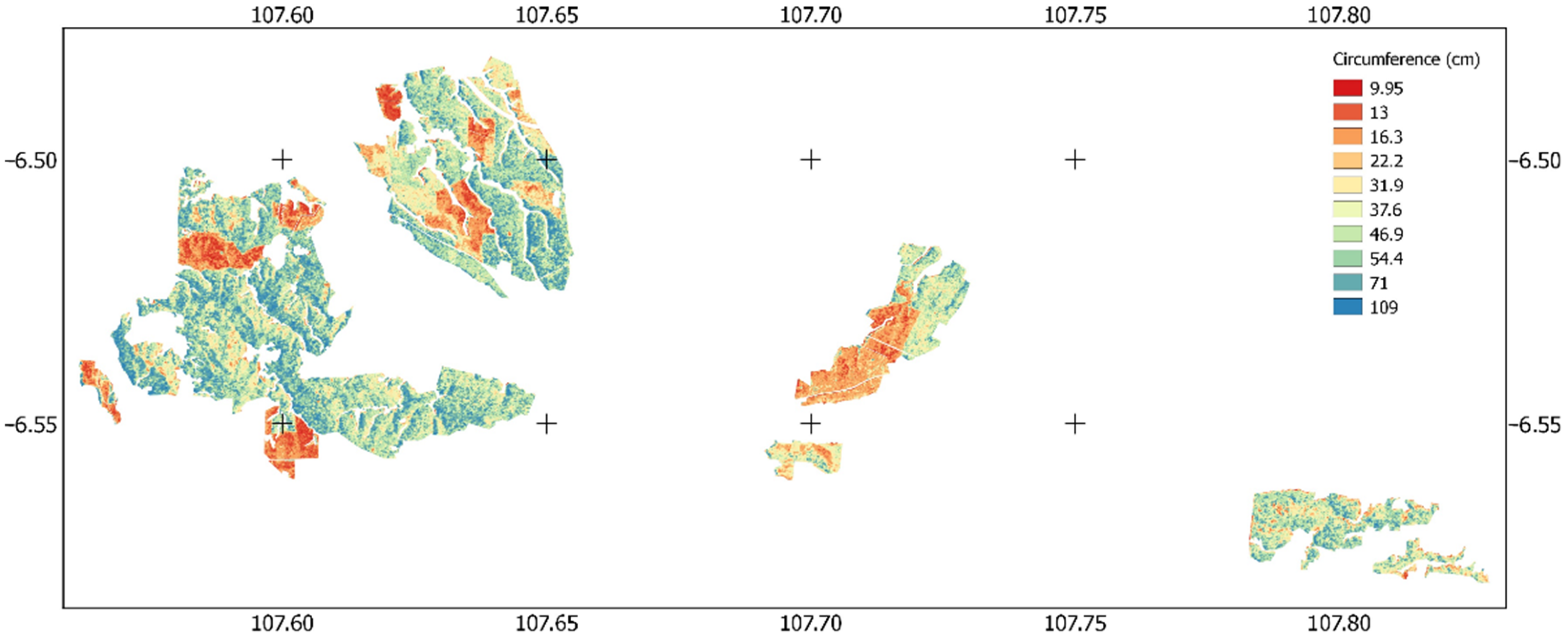
3.4. Prediction
4. Discussion
5. Conclusions
Author Contributions
Funding
Institutional Review Board Statement
Informed Consent Statement
Data Availability Statement
Acknowledgments
Conflicts of Interest
References
- Khatun, R.; Reza, M.I.H.; Moniruzzaman, M.; Yaakob, Z. Sustainable oil palm industry: The possibilities. Renew. Sustain. Energy Rev. 2017, 76, 608–619. [Google Scholar] [CrossRef]
- Castel, T.; Guerra, F.; Caraglio, Y.; Houllier, F. Retrieval biomass of a large Venezuelan pine plantation using JERS-1 SAR data. Analysis of forest structure impact on radar signature. Remote Sens. Environ. 2002, 79, 30–41. [Google Scholar] [CrossRef]
- Allen, M.G.; Burkhart, H.E. A comparison of alternative data sources for modeling site index in loblolly pine plantations. Can. J. For. Res. 2015, 45, 1026–1033. [Google Scholar] [CrossRef]
- Avtar, R.; Suab, S.A.; Syukur, M.S.; Korom, A.; Umarhadi, D.A.; Yunus, A.P. Assessing the influence of UAV altitude on extracted biophysical parameters of young oil palm. Remote Sens. 2020, 12, 3030. [Google Scholar] [CrossRef]
- Azuan, N.H.; Khairunniza-Bejo, S.; Abdullah, A.F.; Kassim, M.S.M.; Ahmad, D. Analysis of Changes in Oil Palm Canopy Architecture from Basal Stem Rot Using Terrestrial Laser Scanner. Plant Dis. 2019, 103, 3218–3225. [Google Scholar] [CrossRef] [Green Version]
- Kobayashi, S.; Omura, Y.; Sanga-Ngoie, K.; Yamaguchi, Y.; Widyorini, R.; Fujita, M.S.; Supriadi, B.; Kawai, S. Yearly variation of Acacia plantation forests obtained by polarimetric analysis of ALOS PALSAR data. IEEE J. Sel. Top. Appl. Earth Obs. Remote Sens. 2015, 8, 5294–5304. [Google Scholar] [CrossRef]
- Broich, M.; Hansen, M.C.; Potapov, P.; Adusei, B.; Lindquist, E.; Stehman, S.V. Time-series analysis of multi-resolution optical imagery for quantifying forest cover loss in Sumatra and Kalimantan, Indonesia. Int. J. Appl. Earth Obs. Geoinf. 2011, 13, 277–291. [Google Scholar] [CrossRef]
- Miettinen, J.; Liew, S.C. Separability of insular Southeast Asian woody plantation species in the 50 m resolution ALOS PALSAR mosaic product. Remote Sens. Lett. 2011, 2, 299–307. [Google Scholar] [CrossRef]
- Abdel-Rahman, E.M.; Mutanga, O.; Adam, E.; Ismail, R. Detecting Sirex noctilio grey-attacked and lightning-struck pine trees using airborne hyperspectral data, random forest and support vector machines classifiers. ISPRS J. Photogramm. Remote Sens. 2014, 88, 48–59. [Google Scholar] [CrossRef]
- Smigaj, M.; Gaulton, R.; Suárez, J.C.; Barr, S.L. Combined use of spectral and structural characteristics for improved red band needle blight detection in pine plantation stands. For. Ecol. Manag. 2019, 434, 213–223. [Google Scholar] [CrossRef]
- Varo-Martínez, M.Á.; Navarro-Cerrillo, R.M. Stand delineation of Pinus sylvestris L. plantations suffering decline processes based on biophysical tree crown variables: A necessary tool for adaptive silviculture. Remote Sens. 2021, 13, 436. [Google Scholar] [CrossRef]
- Amirruddin, A.D.; Muharam, F.M.; Ismail, M.H.; Tan, N.P.; Ismail, M.F. Hyperspectral spectroscopy and imbalance data approaches for classification of oil palm’s macronutrients observed from frond 9 and 17. Comput. Electron. Agric. 2020, 178, 105768. [Google Scholar] [CrossRef]
- Schnell, S.; Kleinn, C.; Ståhl, G. Monitoring trees outside forests: A review. Environ. Monit. Assess. 2015, 187, 600. [Google Scholar] [CrossRef] [PubMed]
- Galidaki, G.; Zianis, D.; Gitas, I.; Radoglou, K.; Karathanassi, V.; Tsakiri–Strati, M.; Woodhouse, I.; Mallinis, G. Vegetation biomass estimation with remote sensing: Focus on forest and other wooded land over the Mediterranean ecosystem. Int. J. Remote Sens. 2017, 38, 1940–1966. [Google Scholar] [CrossRef] [Green Version]
- Dube, T.; Mutanga, O. Quantifying the variability and allocation patterns of aboveground carbon stocks across plantation forest types, structural attributes and age in sub-tropical coastal region of KwaZulu Natal, South Africa using remote sensing. Appl. Geogr. 2015, 64, 55–65. [Google Scholar] [CrossRef]
- Dong, J.; Xiao, X.; Chen, B.; Torbick, N.; Jin, C.; Zhang, G.; Biradar, C. Mapping deciduous rubber plantations through integration of PALSAR and multi-temporal Landsat imagery. Remote Sens. Environ. 2013, 134, 392–402. [Google Scholar] [CrossRef]
- Dibs, H.; Idrees, M.O.; Alsalhin, G.B.A. Hierarchical classification approach for mapping rubber tree growth using per-pixel and object-oriented classifiers with SPOT-5 imagery. Egypt. J. Remote Sens. Space Sci. 2017, 20, 21–30. [Google Scholar] [CrossRef]
- Li, Z.; Fox, J.M. Mapping rubber tree growth in mainland Southeast Asia using time-series MODIS 250 m NDVI and statistical data. Appl. Geogr. 2012, 32, 420–432. [Google Scholar] [CrossRef]
- Kou, W.; Xiao, X.; Dong, J.; Gan, S.; Zhai, D.; Zhang, G.; Qin, Y.; Li, L. Mapping deciduous rubber plantation areas and stand ages with PALSAR and landsat images. Remote Sens. 2015, 7, 1048–1073. [Google Scholar] [CrossRef] [Green Version]
- Trisasongko, B.H.; Panuju, D.R.; Paull, D.J.; Jia, X.; Griffin, A.L. Comparing six pixel-wise classifiers for tropical rural land cover mapping using four forms of fully polarimetric SAR data. Int. J. Remote Sens. 2017, 38, 3274–3293. [Google Scholar] [CrossRef]
- Trisasongko, B.H. Mapping stand age of rubber plantation using ALOS-2 polarimetric SAR data. Eur. J. Remote Sens. 2017, 50, 64–76. [Google Scholar] [CrossRef] [Green Version]
- Trisasongko, B.H. Mapping Stand Age of Indonesian Rubber Plantation Using Fully Polarimetric L-Band Synthetic Aperture Radar. In Advances in Remote Sensing for Natural Resource Monitoring; John & Wiley & Sons, Ltd.: Hoboken, NJ, USA, 2021; pp. 43–57. [Google Scholar]
- Trisasongko, B.H.; Paull, D.J. L-band SAR for estimating aboveground biomass of rubber plantation in Java Island, Indonesia. Geocarto Int. 2020, 35, 1327–1342. [Google Scholar] [CrossRef]
- Azizan, F.A.; Kiloes, A.M.; Astuti, I.S.; Aziz, A.A. Application of optical remote sensing in rubber plantations: A systematic review. Remote Sens. 2021, 13, 429. [Google Scholar] [CrossRef]
- Bickel, S.H.; Bates, R.H.T. Effects of magneto-ionic propagation on the polarization scattering matrix. Proc. IEEE 1965, 53, 1089–1091. [Google Scholar] [CrossRef]
- Freeman, A.; Saatchi, S.S. On the detection of Faraday rotation in linearly polarized L-band SAR backscatter signatures. IEEE Trans. Geosci. Remote Sens. 2004, 42, 1607–1616. [Google Scholar] [CrossRef]
- Aghababaee, H.; Sahebi, M.R. Incoherent target scattering decomposition of polarimetric SAR data based on vector model roll-invariant parameters. IEEE Trans. Geosci. Remote Sens. 2016, 54, 4392–4401. [Google Scholar] [CrossRef]
- Bhattacharya, A.; Singh, G.; Manickam, S.; Yamaguchi, Y. An Adaptive General Four-Component Scattering Power Decomposition with Unitary Transformation of Coherency Matrix (AG4U). IEEE Geosci. Remote Sens. Lett. 2015, 12, 2110–2114. [Google Scholar] [CrossRef]
- Singh, G.; Yamaguchi, Y. Model-Based Six-Component Scattering Matrix Power Decomposition. IEEE Trans. Geosci. Remote Sens. 2018, 56, 5687–5704. [Google Scholar] [CrossRef]
- Singh, G.; Yamaguchi, Y.; Park, S.E. General four-component scattering power decomposition with unitary transformation of coherency matrix. IEEE Trans. Geosci. Remote Sens. 2013, 51, 3014–3022. [Google Scholar] [CrossRef]
- Cloude, S.R.; Pottier, E. An entropy based classification scheme for land applications of polarimetric SAR. IEEE Trans. Geosci. Remote Sens. 1997, 35, 68–78. [Google Scholar] [CrossRef]
- Freeman, A.; Durden, S.L. A three-component scattering model for polarimetric SAR data. IEEE Trans. Geosci. Remote Sens. 1998, 36, 963–973. [Google Scholar] [CrossRef] [Green Version]
- Yamaguchi, Y.; Moriyama, T.; Ishido, M.; Yamada, H. Four-component scattering model for polarimetric SAR image decomposition. IEEE Trans. Geosci. Remote Sens. 2005, 43, 1699–1706. [Google Scholar] [CrossRef]
- Nawar, S.; Buddenbaum, H.; Hill, J.; Kozak, J. Modeling and mapping of soil salinity with reflectance spectroscopy and landsat data using two quantitative methods (PLSR and MARS). Remote Sens. 2014, 6, 10813–10834. [Google Scholar] [CrossRef] [Green Version]
- Migolet, P.; Goïta, K. Evaluation of FORMOSAT-2 and planetscope imagery for aboveground oil palm biomass estimation in a mature plantation in the Congo Basin. Remote Sens. 2020, 12, 2926. [Google Scholar] [CrossRef]
- López-Serrano, P.M.; Corral-Rivas, J.J.; Díaz-Varela, R.A.; álvarez-González, J.G.; López-Sánchez, C.A. Evaluation of radiometric and atmospheric correction algorithms for aboveground forest biomass estimation using landsat 5 TM data. Remote Sens. 2016, 8, 369. [Google Scholar] [CrossRef] [Green Version]
- García, G.A.; Venturini, V.; Brogioni, M.; Walker, E.; Rodríguez, L. Soil moisture estimation over flat lands in the Argentinian Pampas region using Sentinel-1A data and non-parametric methods. Int. J. Remote Sens. 2019, 40, 3689–3720. [Google Scholar] [CrossRef]
- Nawar, S.; Munnaf, M.A.; Mouazen, A.M. Machine learning based on-line prediction of soil organic carbon after removal of soil moisture effect. Remote Sens. 2020, 12, 1308. [Google Scholar] [CrossRef] [Green Version]
- Sonobe, R.; Yamashita, H.; Nofrizal, A.Y.; Seki, H.; Morita, A.; Ikka, T. Use of spectral reflectance from a compact spectrometer to assess chlorophyll content in Zizania latifolia. Geocarto Int. 2021, 1–13. Available online: https://doi.org/10.1080/10106049.2021.1914747 (accessed on 16 March 2022). [CrossRef]
- Rahimikhoob, A. Comparison of M5 Model Tree and Artificial Neural Network’s Methodologies in Modelling Daily Reference Evapotranspiration from NOAA Satellite Images. Water Resour. Manag. 2016, 30, 3063–3075. [Google Scholar] [CrossRef]
- Vapnik, V.N. The Nature of Statistical Learning Theory, 2nd ed.; Springer Verlag: New York, NY, USA, 2000. [Google Scholar]
- Breiman, L. Random forests. Mach. Learn. 2001, 45, 5–32. [Google Scholar] [CrossRef] [Green Version]
- Deng, H.; Runger, G. Gene selection with guided regularized random forest. Pattern Recognit. 2013, 46, 3483–3489. [Google Scholar] [CrossRef] [Green Version]
- Hothorn, T.; Hornik, K.; Zeileis, A. Unbiased recursive partitioning: A conditional inference framework. J. Comput. Graph. Stat. 2006, 15, 651–674. [Google Scholar] [CrossRef] [Green Version]
- Braswell, B.H.; Hagen, S.C.; Frolking, S.E.; Salas, W.A. A multivariable approach for mapping sub-pixel land cover distributions using MISR and MODIS: Application in the Brazilian Amazon region. Remote Sens. Environ. 2003, 87, 243–256. [Google Scholar] [CrossRef]
- Bui, D.T.; Pradhan, B.; Lofman, O.; Revhaug, I.; Dick, Ø.B. Regional prediction of landslide hazard using probability analysis of intense rainfall in the Hoa Binh province, Vietnam. Nat. Hazards 2013, 66, 707–730. [Google Scholar] [CrossRef]
- Filgueiras, R.; Mantovani, E.C.; Dias, S.H.B.; Filho, E.I.F.; Cunha, F.F.D.; Neale, C.M.U. New approach to determining the surface temperature without thermal band of satellites. Eur. J. Agron. 2019, 106, 12–22. [Google Scholar] [CrossRef]
- Maimaitijiang, M.; Ghulam, A.; Sidike, P.; Hartling, S.; Maimaitiyiming, M.; Peterson, K.; Shavers, E.; Fishman, J.; Peterson, J.; Kadam, S.; et al. Unmanned Aerial System (UAS)-based phenotyping of soybean using multi-sensor data fusion and extreme learning machine. ISPRS J. Photogramm. Remote Sens. 2017, 134, 43–58. [Google Scholar] [CrossRef]
- Feng, Z.; Huang, G.; Chi, D. Classification of the complex agricultural planting structure with a semi-supervised extreme learning machine framework. Remote Sens. 2020, 12, 3708. [Google Scholar] [CrossRef]
- Maimaitiyiming, M.; Sagan, V.; Sidike, P.; Kwasniewski, M.T. Dual activation function-based Extreme Learning Machine (ELM) for estimating grapevine berry yield and quality. Remote Sens. 2019, 11, 740. [Google Scholar] [CrossRef] [Green Version]
- Hong, Y.; Chen, S.; Zhang, Y.; Chen, Y.; Yu, L.; Liu, Y.; Liu, Y.; Cheng, H.; Liu, Y. Rapid identification of soil organic matter level via visible and near-infrared spectroscopy: Effects of two-dimensional correlation coefficient and extreme learning machine. Sci. Total Environ. 2018, 644, 1232–1243. [Google Scholar] [CrossRef]
- Chen, T.; Guestrin, C. XGBoost: A scalable tree boosting system. In Proceedings of the 22nd ACM SIGKDD International Conference on Knowledge Discovery and Data Mining, San Francisco, CA, USA, 13–16 August 2016; pp. 785–794. [Google Scholar]
- Buthelezi, M.N.M.; Lottering, R.T.; Hlatshwayo, S.T.; Peerbhay, K. Comparing rotation forests and extreme gradient boosting for monitoring drought damage on KwaZulu-Natal commercial forests. Geocarto Int. 2020, 1–24. Available online: https://doi.org/10.1080/10106049.2020.1852612 (accessed on 16 March 2022). [CrossRef]
- Pham, T.D.; Yokoya, N.; Xia, J.; Ha, N.T.; Le, N.N.; Nguyen, T.T.T.; Dao, T.H.; Vu, T.T.P.; Pham, T.D.; Takeuchi, W. Comparison of machine learning methods for estimating mangrove above-ground biomass using multiple source remote sensing data in the red river delta biosphere reserve, Vietnam. Remote Sens. 2020, 12, 1334. [Google Scholar] [CrossRef] [Green Version]
- Weksler, S.; Rozenstein, O.; Haish, N.; Moshelion, M.; Wallach, R.; Ben-Dor, E. Detection of potassium deficiency and momentary transpiration rate estimation at early growth stages using proximal hyperspectral imaging and extreme gradient boosting. Sensors 2021, 21, 958. [Google Scholar] [CrossRef] [PubMed]
- Neumann, M.; Saatchi, S.S.; Ulander, L.M.H.; Fransson, J.E.S. Assessing performance of L- and P-band polarimetric interferometric SAR data in estimating boreal forest above-ground biomass. IEEE Trans. Geosci. Remote Sens. 2012, 50, 714–726. [Google Scholar] [CrossRef]
- Charoenjit, K.; Zuddas, P.; Allemand, P.; Pattanakiat, S.; Pachana, K. Estimation of biomass and carbon stock in Para rubber plantations using object-based classification from Thaichote satellite data in Eastern Thailand. J. Appl. Remote Sens. 2015, 9, 96072. [Google Scholar] [CrossRef] [Green Version]
- Pope, K.O.; Rey-Benayas, J.M.; Paris, J.F. Radar remote sensing of forest and wetland ecosystems in the Central American tropics. Remote Sens. Environ. 1994, 48, 205–219. [Google Scholar] [CrossRef]
- Mureriwa, N.; Adam, E.; Sahu, A.; Tesfamichael, S. Examining the spectral separability of prosopis glandulosa from co-existent species using field spectral measurement and guided regularized random forest. Remote Sens. 2016, 8, 144. [Google Scholar] [CrossRef] [Green Version]
- Sánchez-Ruiz, S.; Moreno-Martínez, Á.; Izquierdo-Verdiguier, E.; Chiesi, M.; Maselli, F.; Gilabert, M.A. Growing stock volume from multi-temporal landsat imagery through google earth engine. Int. J. Appl. Earth Obs. Geoinf. 2019, 83, 101913. [Google Scholar] [CrossRef]
- Mourtzinis, S.; Edreira, J.I.R.; Grassini, P.; Roth, A.C.; Casteel, S.N.; Ciampitti, I.A.; Kandel, H.J.; Kyveryga, P.M.; Licht, M.A.; Lindsey, L.E.; et al. Sifting and winnowing: Analysis of farmer field data for soybean in the US North-Central region. Field Crops Res. 2018, 221, 130–141. [Google Scholar] [CrossRef]
- Adugna, T.; Xu, W.; Fan, J. Comparison of Random Forest and Support Vector Machine Classifiers for Regional Land Cover Mapping Using Coarse Resolution FY-3C Images. Remote Sens. 2022, 14, 574. [Google Scholar] [CrossRef]
- Geng, L.; Che, T.; Ma, M.; Tan, J.; Wang, H. Corn biomass estimation by integrating remote sensing and long-term observation data based on machine learning techniques. Remote Sens. 2021, 13, 2352. [Google Scholar] [CrossRef]
- Adab, H.; Morbidelli, R.; Saltalippi, C.; Moradian, M.; Ghalhari, G.A.F. Machine learning to estimate surface soil moisture from remote sensing data. Water 2020, 12, 3223. [Google Scholar] [CrossRef]
- Nitze, I.; Schulthess, U.; Asche, H. Comparison of machine learning algorithms Random Forest, Artificial Neural Networks and Support Vector Machine to Maximum Likelihood for supervised crop type classification. In Proceedings of the GEOBIA 4, Rio de Janeiro, Brazil, 7–9 May 2012; pp. 35–40. [Google Scholar]
- Barrett, B.; Nitze, I.; Green, S.; Cawkwell, F. Assessment of multi-temporal, multi-sensor radar and ancillary spatial data for grasslands monitoring in Ireland using machine learning approaches. Remote Sens. Environ. 2014, 152, 109–124. [Google Scholar] [CrossRef] [Green Version]
- Lawrence, R.L.; Moran, C.J. The AmericaView classification methods accuracy comparison project: A rigorous approach for model selection. Remote Sens. Environ. 2015, 170, 115–120. [Google Scholar] [CrossRef]
- Adam, E.; Deng, H.; Odindi, J.; Abdel-Rahman, E.M.; Mutanga, O. Detecting the early stage of phaeosphaeria leaf spot infestations in maize crop using in situ hyperspectral data and guided regularized random forest algorithm. J. Spectrosc. 2017, 2017, 6961387. [Google Scholar] [CrossRef]
- Sai Bharadwaj, P.; Kumar, S.; Kushwaha, S.P.S.; Bijker, W. Polarimetric scattering model for estimation of above ground biomass of multilayer vegetation using ALOS-PALSAR quad-pol data. Phys. Chem. Earth 2015, 83–84, 187–195. [Google Scholar] [CrossRef]
- Pu, W. SAE-Net: A Deep Neural Network for SAR Autofocus. IEEE Trans. Geosci. Remote Sens. 2022, 60, 5220714. [Google Scholar] [CrossRef]


| Model Name | Abbreviation | RMSE | R2 |
|---|---|---|---|
| Multivariate Adaptive Regression Splines | MARS | 10.72 | 0.65 |
| Cubist | Cub | 12.05 | 0.70 |
| Weka-M5 | M5 | 13.88 | 0.64 |
| Bayesian Regularized Neural Networks | NNbr | 14.56 | 0.65 |
| Extreme Learning Machine | NNelm | 15.61 | 0.51 |
| Random Forests | RF | 9.86 | 0.82 |
| Regularized RF | RFg | 9.48 | 0.81 |
| Conditional Inference RF | RFc | 12.75 | 0.75 |
| Support Vector Machine with RBF kernel | SVMrb | 8.82 | 0.77 |
| Extreme Gradient Boosting | GBMxgb | 11.29 | 0.82 |
| Freeman–Durden | Yamaguchi | Singh | ||||
|---|---|---|---|---|---|---|
| Models | RMSE | R2 | RMSE | R2 | RMSE | R2 |
| MARS | 17.69 | 0.84 | 16.23 | 0.80 | 16.50 | 0.78 |
| Cub | 12.05 | 0.70 | 12.05 | 0.70 | 12.05 | 0.70 |
| M5 | 13.88 | 0.64 | 13.88 | 0.64 | 13.88 | 0.64 |
| NNbr | 14.56 | 0.65 | 14.56 | 0.65 | 14.56 | 0.65 |
| NNelm | 18.27 | 0.74 | 17.13 | 0.79 | 18.08 | 0.82 |
| RF | 12.14 | 0.80 | 10.65 | 0.80 | 8.97 | 0.89 |
| RFg | 11.52 | 0.81 | 10.24 | 0.81 | 8.31 | 0.91 |
| RFc | 9.63 | 0.81 | 11.89 | 0.61 | 11.60 | 0.60 |
| SVMrb | 11.28 | 0.65 | 10.22 | 0.67 | 9.70 | 0.71 |
| GBMxgb | 9.50 | 0.81 | 18.40 | 0.66 | 10.13 | 0.86 |
| Abbreviation | RMSE | R2 |
|---|---|---|
| MARS | 15.60 | 0.51 |
| Cub | 19.66 | 0.37 |
| M5 | 12.04 | 0.73 |
| NNbr | 14.56 | 0.65 |
| NNelm | 20.66 | 0.17 |
| RF | 8.82 | 0.86 |
| RFg | 9.69 | 0.83 |
| RFc | 15.03 | 0.64 |
| SVMrb | 17.72 | 0.06 |
| GBMxgb | 8.58 | 0.92 |
Publisher’s Note: MDPI stays neutral with regard to jurisdictional claims in published maps and institutional affiliations. |
© 2022 by the authors. Licensee MDPI, Basel, Switzerland. This article is an open access article distributed under the terms and conditions of the Creative Commons Attribution (CC BY) license (https://creativecommons.org/licenses/by/4.0/).
Share and Cite
Trisasongko, B.H.; Panuju, D.R.; Griffin, A.L.; Paull, D.J. Fully Polarimetric L-Band Synthetic Aperture Radar for the Estimation of Tree Girth as a Representative of Stand Productivity in Rubber Plantations. Geographies 2022, 2, 173-185. https://doi.org/10.3390/geographies2020012
Trisasongko BH, Panuju DR, Griffin AL, Paull DJ. Fully Polarimetric L-Band Synthetic Aperture Radar for the Estimation of Tree Girth as a Representative of Stand Productivity in Rubber Plantations. Geographies. 2022; 2(2):173-185. https://doi.org/10.3390/geographies2020012
Chicago/Turabian StyleTrisasongko, Bambang H., Dyah R. Panuju, Amy L. Griffin, and David J. Paull. 2022. "Fully Polarimetric L-Band Synthetic Aperture Radar for the Estimation of Tree Girth as a Representative of Stand Productivity in Rubber Plantations" Geographies 2, no. 2: 173-185. https://doi.org/10.3390/geographies2020012
APA StyleTrisasongko, B. H., Panuju, D. R., Griffin, A. L., & Paull, D. J. (2022). Fully Polarimetric L-Band Synthetic Aperture Radar for the Estimation of Tree Girth as a Representative of Stand Productivity in Rubber Plantations. Geographies, 2(2), 173-185. https://doi.org/10.3390/geographies2020012