Article

Spatial and Temporal Change of Land Cover in Protected Areas in Malawi: Implications for Conservation Management

by
Daniel Kpienbaareh
*,
Evans Sumabe Batung
and
Isaac Luginaah
Department of Geography and Environment, Social Science Centre, Western University, London, ON N6A 5C2, Canada
*
Author to whom correspondence should be addressed.
Geographies 2022, 2(1), 68-86; https://doi.org/10.3390/geographies2010006
Submission received: 8 January 2022 / Revised: 6 February 2022 / Accepted: 9 February 2022 / Published: 12 February 2022
(This article belongs to the Special Issue Applying Remotely Sensed Imagery in Natural Resource Management)

Abstract

:
Protected areas (PAs) transform over time due to natural and anthropogenic processes, resulting in the loss of biodiversity and ecosystem services. As current and projected climatic trends are poised to pressurize the sustainability of PAs, analyses of the existing perturbations are crucial for providing valuable insights that will facilitate conservation management. In this study, land cover change, landscape characteristics, and spatiotemporal patterns of the vegetation intensity in the Kasungu National Park (area = 2445.10 km2) in Malawi were assessed using Landsat data (1997, 2008 and 2018) in a Fuzzy K-Means unsupervised classification. The findings reveal that a 21.12% forest cover loss occurred from 1997 to 2018: an average annual loss of 1.09%. Transition analyses of the land cover changes revealed that forest to shrubs conversion was the main form of land cover transition, while conversions from shrubs (3.51%) and bare land (3.48%) to forest over the two decades were comparatively lower, signifying a very low rate of forest regeneration. The remaining forest cover in the park was aggregated in a small land area with dissimilar landscape characteristics. Vegetation intensity and vigor were lower mainly in the eastern part of the park in 2018. The findings have implications for conservation management in the context of climate change and the growing demand for ecosystem services in forest-dependent localities.

1. Introduction

Landscapes in protected areas such as National Parks and watersheds change because of natural disturbances, ecological processes, and anthropogenic activities [1]. However, anthropogenic activities by far pose the most significant threat to biodiversity in protected lands [2,3,4]. Hence, it is necessary to continually monitor and map the land cover dynamics within and around protected areas to inform forest resource managers of the most appropriate regulatory measures to adopt for the conservation of biodiversity and to increase precision in the utility of such measures [5]. Making such management decisions is relevant because, in addition to being an essential source of livelihood and income for local communities [6], protected areas also serve as carbon sinks that help to mitigate climate change [7]. Additionally, forests are a vital source of revenue for economic development through ecotourism in many countries [6].
Changes in protected areas can have a dual effect on biodiversity; they may enable some organisms to thrive (by preying on other organisms easily) while making the landscape uninhabitable for others (by exposing them to expected risks/shocks) [8]. The frequency and extent of disturbances in protected areas are a function of the structural and functional attributes of the ecosystem [9,10,11]. Intricate interdependence and interactions between change patterns and the landscape structure over time create complex dynamic and unpredictable mosaics [12] that impact the integrity of ecosystems and ecosystem services—the benefits that humans derive from healthy ecosystems [13]. In particular, land-use practices in and around conservation areas may influence change patterns by reducing the amount of vegetation cover and their contiguity, which creates complex unnatural shapes or uniform natural patterns that may affect the ability of biodiversity to thrive [14,15].
In already fragile ecosystems, disturbances escalate the rate of degradation, which may further aggravate the existing precarious conditions in the habitats. Monitoring landscape changes in such protected areas over time will, therefore, provide crucial information for management regimes and restoration of stressed ecosystems, as well as increase spatial heterogeneity of vegetation [16,17] to provide conducive habitats for wildlife and other secondary dependents such as humans. There are about 8568 protected areas in Africa, constituting 14.18% of its total land [18]. Unfortunately, in many of these protected areas, there have not been sufficient detailed analyses to provide the crucial information needed to inform management decisions even though rapid changes resulting from, especially anthropogenic activities, is the leading cause of the loss of biodiversity on the continent [19,20,21].
Remote sensing represents a cost-effective geospatial tool for monitoring landscape changes in protected lands to provide valuable data for ecosystem management [22,23]. Remote sensing techniques, combined with landscape metrics and geostatistical modelling are effective for documenting the nuances of deforestation rates, characteristics of landscape structure and patterns of change, and the demand and supply of ecosystem services. Results from remote sensing analyses can also provide critical data for addressing questions concerning the ecological conditions of an area, as well as the perturbations that modify the phenological patterns of vegetation [24,25]. While other scholars have applied these geospatial techniques to understand various landscape changes [26,27,28], these studies have focused mostly on forest cover change on a broader scale. Yet, protected areas, which are created primarily to protect and sustain biodiversity, have not received similar widespread attention, especially in sub-Saharan Africa, despite evidence of growing populations density around such lands.
In this study, satellite data, landscape metrics, and geostatistical modelling were deployed to analyze land cover change with a focus on forest cover, landscape characteristics, and the intensity and spatiotemporal pattern of vegetation cover dynamics in the Kasungu National Park (KNP) in western-central Malawi. Our research in a protected area complements studies at the global [29,30], continental [31], national [32], and regional scales [33] by demonstrating that remotely sensed data can be used to explore the intricate details and nuances of changing patterns and transitions in land cover to influence conservation management decisions. Even though landscape changes are apparent in KNP, research on the area has mainly focused on travel and tourism [34,35], the economic benefits of the park to fringe communities [36], and plant and animal censuses [37,38]. As such, little is known about the structural and potentially functional changes the park has undergone over the years. As climate change and variability intensifies, several questions regarding the quantity of forest cover, ecological integrity and sustainability of protected areas continue to surface. For instance, crucial questions include: has the forest cover increased or decreased over the years? Are there any unnatural shapes/patterns of vegetation cover developing? If so, what are the implications of these changes to biodiversity? This study addresses some of these pertinent questions.

Protected Areas in Malawi

Malawi is endowed with several natural ecosystems. With a total area of 118,860 km2, about 27,190 km2 of the land constitutes dry land, and the remaining land area is covered by water [39]. About 11% of the total dry land area is designated as national parks and wildlife reserves while an additional 10% is forest reserves and protected hillslopes. The national parks and protected areas, which are spread across the country, include Nyika National Park and Vwaza Marsh Wildlife Reserve in the north of Malawi; Kasungu National Park and Nkhotakota Wildlife Reserve in central Malawi; Liwonde and Lengwe National Parks and Majete and Mwabvi Wildlife Reserves in the southern region of Malawi; and the Lake Malawi National Park. The size of protected land implies that Malawians likely compete for arable land for agricultural and other uses. With a total population of about 17,563,749 which grows at a rate of 2.9% per annum, according to the 2018 Population and Housing Census [40], the competition for land including protected lands will likely be exacerbated in the coming years. The agrarian nature of Malawi, coupled with current population growth trends, suggests dire implications for the future of biodiversity in protected lands.
The Wildlife and Environmental Society of Malawi asserts that protected areas are critical to the livelihoods of rural farmers [39]. As highlighted by political ecologists who research environmental issues in developing countries [41,42], human-environment interdependence often leads to tension between local communities and resource managers because of issues surrounding the access to and utilization of ecosystem services. In Malawi, the high proportion of protected areas often results in poaching and farming in and around such conservation areas, as highlighted by the political ecologists. Rising poverty rates which disproportionately affect rural areas in Malawi [43] suggest increasing pressure on the protected areas [44,45]. Additionally, the rapidly changing climate, as evidenced by recent floods and droughts [46], call for a thorough re-strategizing in management regimes. There is, thus, a need to provide relevant spatial information through regular monitoring to enhance decision-making for efficient and sustainable management. The KNP was chosen as the study area for detailed analysis and to provide a general understanding of protected areas in Malawi for several reasons. Firstly, the KNP is one of the largest parks in Malawi and hosts a wide variety of biodiversity. For example, because the park covers a large area of the Brachystegia and Julbernardia woodlands, it attracts a significant number of elephants (Loxodonta africana) [47]. In addition, a study by Mkanda and Munthali [35] on public attitudes towards the park revealed that increasing anthropogenic pressures on the park are likely due to the need for ecosystem services including bee-keeping, the collection of firewood, mushrooms, and building materials. The wildlife preservation and biodiversity potential of the park, along with the increasing threats of intense exploitation strongly underpins the primary objective of this study as it will provide necessary information concerning management of these biodiversity.

2. Materials and Methods

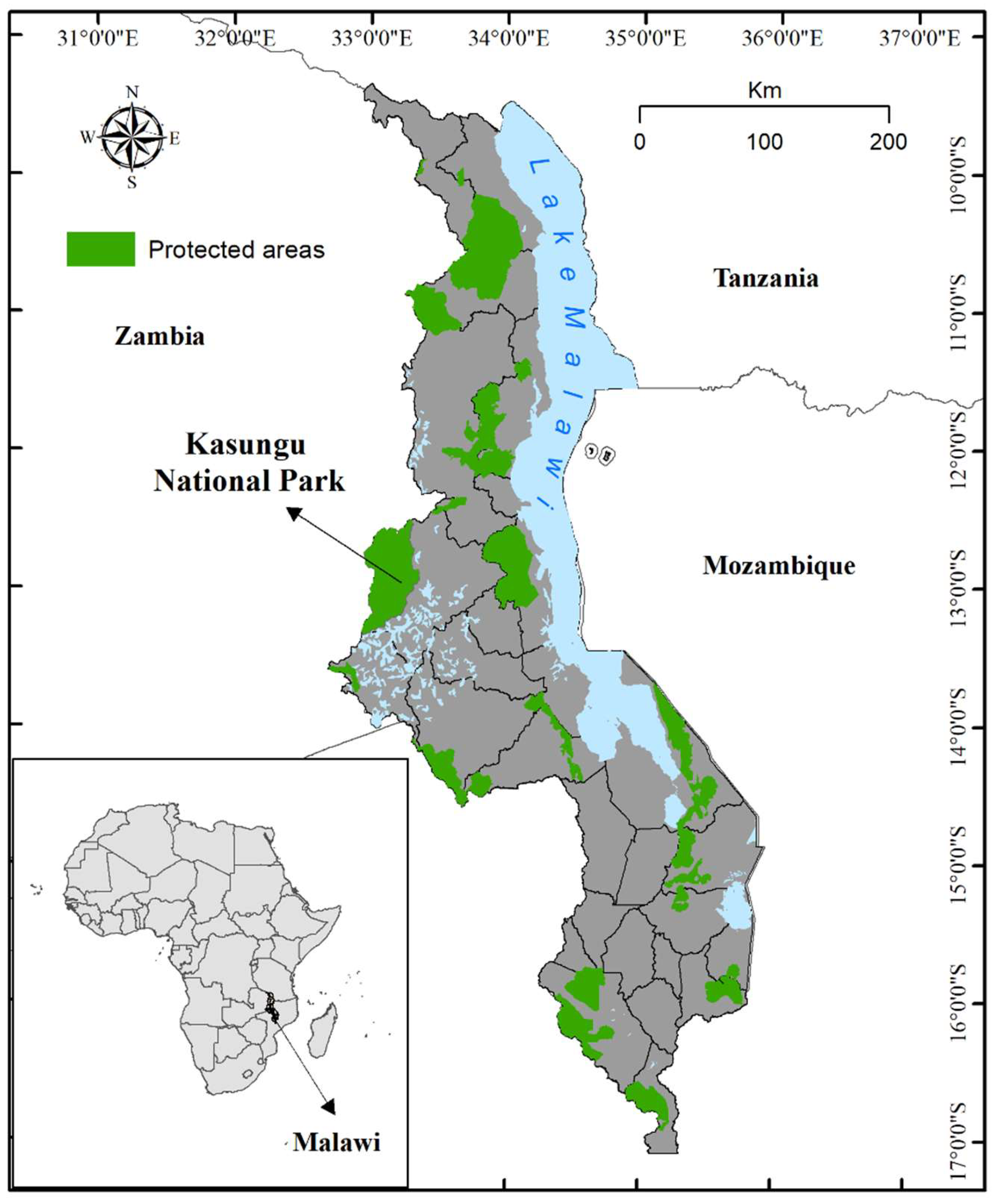
2.1. Study Area Description

The Kasungu National Park (KNP) (Figure 1), located in western-central Malawi, covers an area of 2316 km2 [37]. The vegetation types and composition in the park vary by location and elevation. The plateau areas have deep sandy soils with poor nutrient content and high-water infiltration, and, thus, have a closed-canopy Brachystegia and Julbernardia vegetation (Miombo woodland), which have short to medium height grasses [38]. The plateau dambos (seasonally flooded open grass areas) are flat and sandy, with grasses of medium height. The valley areas, mainly in the central part of the park, have open woodlands, with relatively tall Hyparrhenia grasses [48,49]. The main tree species in this part of the park are of the genera Terminalia, Combretum and Pericopsis.
The variable landscape of the KNP, with elevation ranging between 1000 and 1500 m, partly influences the climatology of the park [50]. The rainy season in the area stretches between October and May, with most rain usually falling in January and February [51]. Mean annual rainfall is about 780 mm [38]. Temperature-wise, June is the coldest month, after which temperatures gradually increase until they reach their highest in November [38]. Despite the relative consistency of atmospheric temperature when compared to other variables, some notable variability does occur. In the hottest month, for instance, maximum temperatures are about 31.3 °C, while the minimum temperatures hover around 19.5 °C [51].
Although estimates of wildlife in the KNP vary, it is generally agreed that animals are relatively concentrated in the valley areas [52]. Wild animals, including elephants, buffalos and waterbucks, comprising 75% of all herbivorous animals in the park, mainly inhabit the valley areas, with more than 50% of these herbivores concentrated in 20% of the total area of the park [52]. A reduction in the forest cover in these concentrated areas could potentially lead to the extinction of weaker species of animals. Smaller animals including roan, zebra, sable and Lichtenstein’s hartebeest also make up about 20% of the total mammal population in the park, with less than 10% of them in the valley areas [52]. Thus, depletion in the vegetation cover in the habitats of the animals could have dire implications for their survival.

2.2. Data Acquisition and Processing

Table 1 describes the characteristics of the Landsat data used in this study, as has been used in other studies that have assessed protected area changes [53]. The image selection and the timing of the years were based on the availability of cloud-free images, as there is high cloud cover in the area during the rainy season [54]. Admittedly, these dry season images may influence the quantity of forest cover and vigor of the vegetation. Given that all the images chosen were all for July, the similarities and differences will likely be uniform across the images, thus providing comparable results. All the images were projected to WGS84_UTM_Zone_36S at 30 m spatial resolution, and geo-rectified to the same coordinate system using seventeen ground control points to ensure spatial coincidence [55]. A Root Mean Square Error (RMSE) of 0.14 was attained for the geo-rectification. Atmospheric correction and haze removal operations were performed to remove dust, smoke, and haze particles that were present in the atmosphere during the time of image capture to enhance local contrast while maintaining the structural information of the original image [56]. The digital numbers were converted to radiance values using gains and offsets contained in the metadata files of the images [57]. Finally, the visible and near infra-red (NIR) bands of the images were selected and composited into a multiband image for use in the classification, while the red and near-infrared (NIR) bands were used for computing the Normalized Difference Vegetation Indices (NDVI). We note that although the spatial resolution of the images was 30 m × 30 m, evidence suggests that the Landsat OLI/TIRS demonstrates higher accuracy in classifying land cover types compared to Landsat 5 TM [58], although studies have shown that both Landsat 5 and 8 have generally produced good classification results that can be compared.

2.3. Land Cover Change Analysis

To derive good results for a land cover classification of remotely sensed images, it is imperative to reduce the number of classes and choose classes that represent markedly distinct land cover types on the landscape [59]. Thus, the three Landsat images were used in a four-class classification schema—forest, shrubs, bare land, and water, to analyze the landscape of the park. The classes were identified based on field knowledge of the park, detailed visual inspection of the landscape from very high resolution images in Google Earth Pro and general guidelines for land use and land cover classification for use with remote sensor data provided by the United States Geological Survey [60]. This comprehensive identification approach was used to reduce uncertainty and confusion among different classes, especially the forest and shrubs classes, as has been done in other studies [58]. The ‘forest class’ comprised matured trees standing individually or in clusters with clearly defined crowns. The ‘shrubs class’ comprised small- to medium-sized perennial woody plant trees with their multiple stems and shorter height, less than 6–10 m tall trees [61], undergrowth, grasses, and re-emerging plants from burning incidents. We considered the ‘bare land class’ as comprising areas with more than 85% exposed land surface either in dried-up waterways, clear-cut areas, roads/tracks, and farmlands mainly at the fringes of the park. The ‘water class’ is composed mainly of three small lakes in the reserve that still have water in them. Global Positioning System (GPS) devices were used to take XY coordinates around these classes as samples in late 2018 as reference data for accuracy assessment of the 2018 image and as reference data for selecting samples for accuracy assessment for the 1997 and 2008 time points. The coordinates in .gpx file format were converted to point feature classes and subsequently to polygons using the ‘point to line tool’ in ArcGIS Pro. These polygons were then used as a guide for selecting the reference data for the original 1997 and 2008 images.
A Fuzzy K-Means unsupervised classification algorithm was used to classify the three images. In a fuzzy clustering [62], each pixel has a degree of belonging to different classes, as in fuzzy logic, rather than belonging exclusively to just one class. Thus, pixels on the edge of a class may be in the class to a lesser degree than pixels in the centre of the class. The Fuzzy K-Means algorithm is based on the fuzzy set theory which makes it possible for uncertainty to be accounted for naturally and realistically during data analysis [63]. The intricate nature of the forest and shrubs in the park detected from field observations means that there is uncertainty between the two classes and hence, the choice of the Fuzzy K-Means algorithm for the classification. A total of twenty (20) clusters were generated in CATALYST Professional software in 5000 iterations and were aggregated into the four classes used in this analysis.
In this study, classification accuracy was assessed using reference samples selected from the original Landsat images as has been applied in other studies [64]. A stratified random sampling strategy was used to select 295 sample polygons from the original images using the polygons generated from the field data for accuracy assessment [58]. The polygons from all the three time points were converted to raster data at the same spatial resolution as the original raster images (30 m × 30 m) and compared with the classified images to create a confusion matrix. Accuracy assessment of the classifications was based on Congalton’s [65] method which involves computing the producer’s, user’s and overall accuracies, as well as their respective Kappa coefficients. The producer’s accuracy is the map accuracy from the map maker’s point of view, while the user’s accuracy is the accuracy from the map user’s point of view. The overall accuracy is usually expressed as a percentage, with 100% accuracy being a perfect classification where all reference sites were correctly classified. The overall accuracy is computed by dividing the total number of correctly classified pixels by the total number of reference pixels. The Kappa on the other hand evaluates how well the classification performed as compared to just randomly assigning values, i.e., did the classification do better than random. The Kappa coefficient ranges from −1 to 1; with a value of 0 indicating that the classification is no better than a random classification. Values close to 1 or −1 indicate that the classification is significantly better or worse than random, respectively. We expect the overall accuracies to be higher than 85% which is often considered the ideal classification accuracy for land cover analysis [60].
For the landscape composition and configuration analysis, the classified images were reclassified into two classes—forest and non-forest (comprising the shrubs, bare land, and water classes). The two classes were used in FRAGSTATS software to compute landscape metrics for assessing the composition and configuration of the park’s landscape for the three time points. The software considers the two reclassified categories as independent classes and computes the metrics for both classes. We did this binary reclassification because some of the landscape metrics cannot be computed with only a single class. Despite this binary re-classification, the outcome of the analysis is not influenced by the values of the other classes—i.e., each class is treated independently by the software.

2.4. Landscape Pattern Analysis

Following McGarigal et al. [66], landscape metrics were used to analyze the temporal pattern of landscape composition and configuration in classified images from 1997, 2008 and 2018. A total of six landscape metrics that could be analyzed, evaluated, and interpreted without any ambiguity [67] were selected for this analysis. We selected these metrics because they quantify fundamental aspects of landscape composition and configuration which are useful descriptors of landscape structure in a wide range of real landscapes [68]. The six metrics are as follows:
  • Clumpiness index (CLUMPY = 0 when the patches are distributed randomly and approach 1 when the patch type is maximally aggregated),
  • Landscape Shape Index (LSI increases without limit as the patch type becomes more disaggregated),
  • Aggregation Index (AI = 0 when the patches are maximally disaggregated and equals 100 when the patches are maximally aggregated into a single compact patch),
  • Patch Density (PD measures the number of patches/100 ha),
  • Shannon’s Diversity Index (SHDI increases when the proportional distribution of area among patch types becomes more equitable), and
  • Largest Patch Index (LPI = percentage of landscape occupied by the largest patch in the ecosystem).
Several studies have adopted these metrics to study fragile ecosystems in landscapes and forest fragmentation as well as their spatial and temporal dynamics [53,69,70,71].

2.5. Spatial Modelling of Vegetation Cover

To assess the spatial patterns of forest cover in the park, NDVI [72], which is related to the leaf area index and fractional vegetation [73] was used. The NDVI for all the three-time points were computed from the following:
N D V I = ( N I R λ R e d λ ) ( N I R λ + R e d λ )
where λ is the centre wavelength of the Landsat 8 OLI/TIRS and Landsat 5 TM sensors (see footnote on Table 1).
NDVI provides information on the health and productivity of vegetation, the fraction of absorbed photosynthetic active radiation intercepted, and biomass and phenological patterns [74], thus, it represents a great information vector for landscape structure and temporal change analyses [75]. As such, the index is useful for identifying patterns of vegetation cover in the park for the three time points. We use ‘vegetation cover’ more broadly here, as opposed to forest cover used in the land cover change analysis and the landscape analysis section above, to include all forests and shrubs in the park because they are all essential for the survival of biodiversity—both animals and plants [76]. Theoretically, the NDVI algorithm cannot discriminate between forests and other forms of vegetation cover when computing values from satellite images.
A semi-variogram analysis was performed to measure the spatial dependence of NDVI values over space and time [77], using 295 randomly selected empirical NDVI values from the NDVI image computed using Equation 1 above. Spatial dependence connotes that below a certain distance threshold, two observations at different locations are statistically dependent on each other (Tobler’s first law of geography; [78]). Through spatial dependence, it is possible to estimate the autocorrelation of NDVI values over distance to provide information on how vegetation amount varies over space (i.e., the intensity of vegetation amount on the landscape). Strong autocorrelation implies high-intensity vegetation cover and vice versa. Observing the patterns of the intensity over time will, therefore, provide information on spatial and temporal variation of vegetation cover due to natural effects and/or anthropogenic activities.
A semi-variogram describes how empirical data are related to each other over space/distance [79]. After exploring the data, a four-step procedure was adopted for the semi-variogram analysis. A linear de-trending procedure was first applied by fitting a plane to the NDVI values to account for medium to long-range spatial anisotropy [53]. Secondly, the data were transformed using the empirical base distribution method and the multiplicative skewing approach because the NDVI data contained negative values. Next, the empirical semi-variogram was calculated for all directions to measure the extent and intensity of geometric anisotropy. Finally, a spherical semi-variogram model (equation 2) was fitted to the de-trended and transformed data. An iterative approach was used to fit semi-variogram models with different parameters to identify the standard model of spatial dependence [80] (results of which are presented here) based on the RMSE values of the models [81]. Mathematically, the model with the smallest RMSE value indicates the one that best fits the data. The spherical semi-variogram is expressed as:
γ 2 ( h ) = C 0 + C 2 [ 3 h a 0 ( h a 0 ) 3 ]
where h is the vector of the directional distance separating two locations, C0 is the nugget or the variability in the empirical data that cannot be explained by the distance between two observations, C is the explained spatial variance, and a 0 is the semi-variogram range. The quantity C 0 + C is the sill (the variance of the data at which the semi-variance is at maximum). The range represents the distance at which two observations are unrelated (i.e., separated by distances greater than the range). Low range values indicate that the total variance of NDVI is expressed in small areas. The ratio of the nugget to total semi-variance (C0/(C0 + C) was computed to measure the strength of spatial autocorrelation between NDVI values. A ratio <0.25 represents a strong autocorrelation, 0.25–0.75 a medium autocorrelation, and >0.75 a weak degree of spatial autocorrelation in the NDVI values [82].
Using both landscape metrics and spatial dependence models in this study allowed us to examine the landscape of the park for the existence of a relationship between the vegetation spatial heterogeneity and the occurrence/spread of disturbance events [53], which may have created clustering/aggregation or disaggregation of forest cover on the landscape. Therefore, we account for essential information that can be generated to more thoroughly understand protected area landscapes.

3. Results

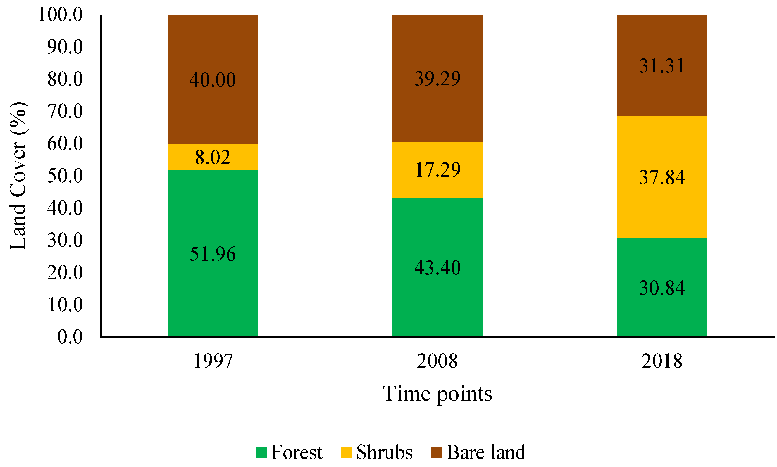
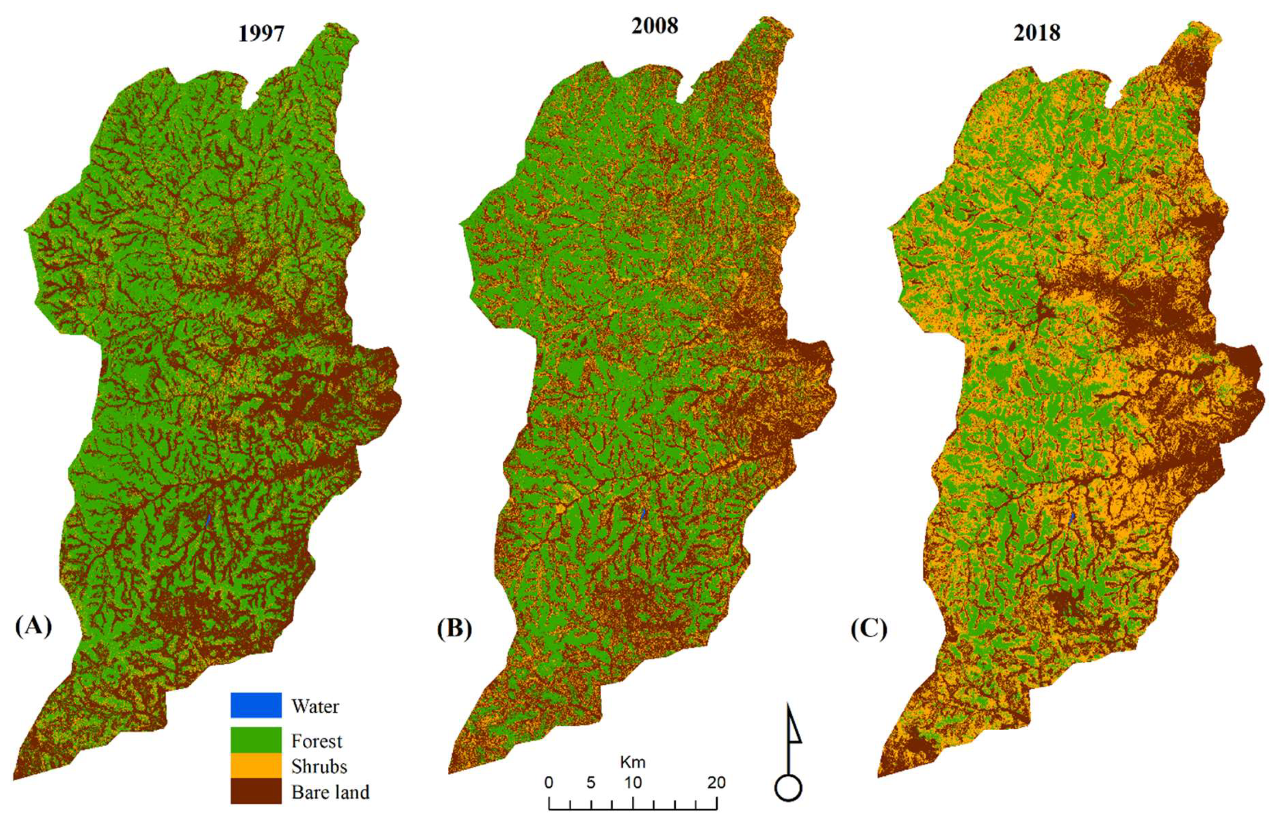
3.1. Image Classification

The results of the producer’s and user’s accuracy assessments are indicated in Table 2. The assessment results for each classified satellite image for 1997, 2008 and 2018 were 92%, 90%, and 93%, respectively, while the corresponding kappa statistics were 0.87, 0.86, and 0.84, respectively. The Landsat 8 OLI/TIRS image which was assessed using the field reference data produced the highest accuracy. All the overall accuracies were higher than the generally accepted minimum of 85% accuracy for an ideal classification in remote sensing, with equally acceptable user’s and producer’s accuracies.
Figure 2 presents the results of the land cover categories in the KNP in percentages. The forest cover consistently decreased from 51.96% of the 2445.10 km2 total land area in 1997 to 43.40% in 2008 and 30.84% in 2018, while the percentage of shrubs increased from 8.02% in 1997 to 17.29% in 2008 and 37.84% in 2018. The percentage of bare land also reduced over this period. Water class was the smallest land cover category in the park but reduced during the period of the study. Overall, there was a 21.12% reduction in forest cover from 1997 to 2018, representing an average annual reduction of 1.09% over the twenty years.
Figure 3 shows the spatial and temporal patterns of land cover categories in the park for the three-time points. There was a noticeable reduction in the amount of forest cover for 1997 compared to 2008 and 2018, while at the same time, the distribution of shrubs increased over the three-time points. Figure 3C also shows the emergence of more bare lands in the northern tip of the park as well as in the eastern part of the map, indicating areas of intense deforestation. There are also areas of bare land, mostly farm plots along the western border of the park which also is the eastern border with Zambia, indicating a notable degree of encroachment by farmers likely from Zambia. The southern tip of the park has also experienced an increase in the amount of bare land in 2018. Overall, however, the distribution of shrubs dominates the park in 2018, possibly an indication that most of the conversions from the forest were to shrubs and that there is likely a high rate of harvesting of forest trees for various livelihood purposes.

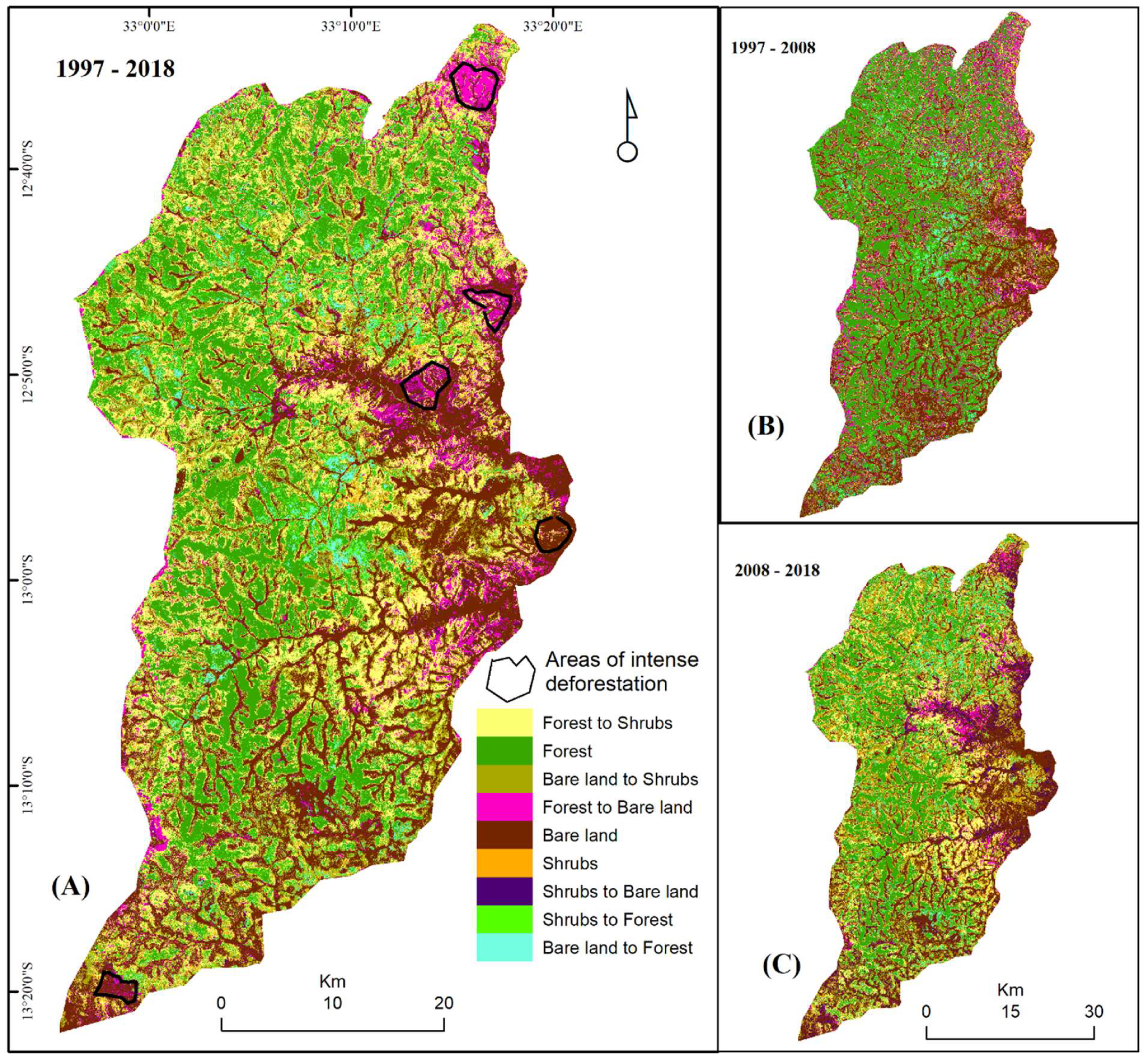
3.2. Transitions of Land Use/Cover Change

Table 3 shows the pattern of land cover transitions between the various categories for the three-time points. The column IDs indicate the transitions from one land cover class (Column 1) to another land cover class (Column 2). The Row IDs show the various permutations of change that occurred in the nearly 21-year period. Column 5 shows the total amount of transition to the ‘To Class’ or persistence of a particular land cover class from 1997 to 2018. The results show that 531.31 km2 of forest transitioned to shrubs from 1997 to 2018 (Row ID 1) while the corresponding conversion from shrubs to forest over the same period was only 85.78 km2 (Row ID 8). At the same time, an additional 156.04Km2 of forest transitioned to bare land in 2018 (Row ID 4), but 321.37 km2 converted to shrubs (Row ID 3). Meanwhile, only 85.04 km2 of bare land transitioned to forests (Row ID 9) over the period.
Figure 4 shows the distribution of changes for the various periods analyzed. Figure 4A shows the overall (1997 to 2018) gains, losses, and persistence of land cover classes in the KNP. It shows areas of gains in forest cover in the central part of the park and the increased emergence of shrubs across the park, likely the effect of natural causes such as droughts or seasonality. Figure 4B and Figure 4C indicate the forest changes for 1997–2008 and 2008–2018 respectively, during which there were areas of intense deforestation.

3.3. Landscape Composition and Configuration

Table 4 highlights the complexities in the structure and shape of changing forest cover over the years. With the CLUMPY, AI and LPI all consistently increasing over the period, there is a strong indication that over the twenty years, the forest patches became more clustered/aggregated. The increasing LPI further confirms that the forest experienced continual clustering. The PD, LSI and SHDI on the other hand consistently decreased, also indicating more disaggregated and diverse forest cover characteristics. The decreasing SHDI indicates dissimilarity in the clustered or aggregated forest clusters. Even though the analysis shows an overall decrease in forest cover, the decreasing SHDI indicates that the remaining forest cover on the landscape has become more diverse, a sign of disproportionate loss in forest cover over the landscape. These seemingly contrasting findings highlight some of the key complexities of such a rapidly changing landscape. Overall, the metrics indicate that by 2018, the landscape of the KNP became more aggregated, but likely partly because the forest reduced and became more concentrated in a smaller area of the park, hence the indication of clumpiness and aggregation.

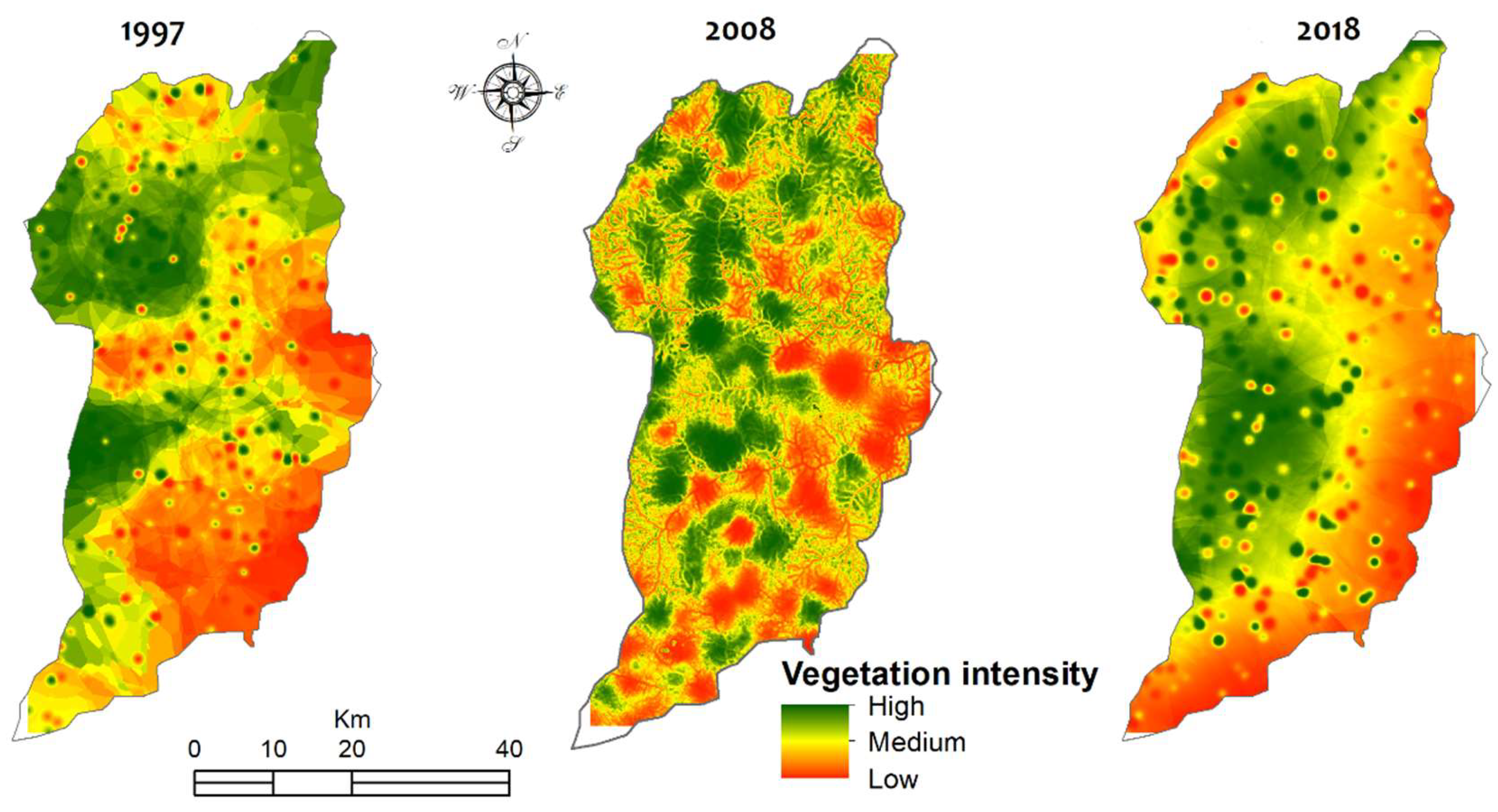
3.4. Intensity and Spatial Pattern of Vegetation Cover

In the semi-variogram analysis, both forest and shrubs were considered as vegetation cover because NDVI computation considers all healthy vegetation in the landscape, which includes both forests and shrubs. The semi-variogram analysis revealed that vegetation exhibited temporal and spatial variability over the study period, as shown by the landscape pattern analysis. The predicted 2018 NDVI produced a negligible nugget effect (Table 5), and a larger sill, indicating a strong spatial autocorrelation between the empirical and predicted values. The autocorrelation indicates high-intensity vegetation cover (high NDVI values surrounded by high values). Compared to 1997, however, the 2008 model produced a larger nugget effect and a relatively smaller sill, even though the nugget was still smaller than the sill, indicating medium autocorrelation. The range, which describes the distance at which the semi-variance stops increasing, was relatively higher in 2018 than in 1997 but smaller in 2008. This means there were fewer patches in 2018 than the other years and more patches in 2008 than in 1997. Overall, the lower range value in 2008 implies small-scale heterogeneity in small areas, with relatively many patches, as revealed by the landscape metrics.
Figure 5 presents the modelled surface of the NDVI values. In 1997, high-intensity NDVI values were concentrated mainly in the northern and southern half of the park, with low intensity in the central part. The intensity was more variable in 2008, producing patches of high intensity interspersed with low intensity, indicating a more fragmented landscape (see Table 4). The 2018 model shows the high intensity of vegetation cover in the eastern part of the park, but with a contiguous patch of high values from the central to the western half of the park. The high clustering of low values in the northern and southern edges reveals a permanent loss of vegetation cover. Overall, the high intensity of NDVI values was more prevalent on higher grounds in comparison to the low-lying areas. Low-intensity values in the northern and southern edges in 2018 coincided with increased forest cover loss, while 2008 revealed patchy/fragmented intensity patterns which reflect our results of the landscape composition and configuration analysis.

4. Discussion

The primary objective of this study was to analyze land cover change, intensity, spatial and temporal patterns of vegetation cover, and landscape composition and configuration in Malawi’s Kasungu National Park (KNP). Such analyses highlight the relevance of remote sensing data and methods for providing detailed information needed for conservation management decisions in protected areas. The results of the classification produced acceptable accuracies (see Table 2) that are generally consistent with other studies involving Landsat image classification [83,84], with the Landsat 8 OLI/TIRS images producing the highest accuracy. According to Poursanidis [58], the higher overall accuracy of the OLI/TIRS image is likely because of the better quality of the Landsat 8 sensor. The study reveals three major characteristics of the KNP: first, consistent with the national deforestation rate of Malawi, there is a high rate of deforestation in KNP, with more of the forest converting to shrubs in 2018 (Table 3 and Figure 4); secondly, there were variations in the composition and configuration of forest cover in the park for 1997, 2008 and 2018 time points as revealed by the landscape metrics (Table 4); and, thirdly, the semi-variogram analysis showed varying temporal patterns of overall vegetation cover, with higher aggregation of vegetation patches observed in 2018 (see Table 5, Figure 5). As demonstrated in this research, and corroborated by other researchers [85,86], a majority of studies have used Landsat TM/ETM+ and OLI/TIRS images to assess changes in and around protected areas, highlighting the utility of these data for making conservation management decisions.
Malawi has a national deforestation rate of about 2.8% or 2500 km2 average annual loss of forest cover [87]. Although our finding of about 1.09% annual loss of forest from 1997 to 2018 is lower than this high rate of deforestation in the country, the findings are, however, consistent with the general assertion that the rate of deforestation in protected areas is often lower than in unprotected areas [88,89], thus justifying the use of protected areas as an effective conservation strategy for biodiversity. Studies [90,91,92,93,94] have reported that other national parks in Malawi face similar high rates of deforestation. According to scholars such as Mauambeta [39] and Lindsey et al. [95], weak enforcement of the law, inadequate funds to deploy law enforcement agents, and the lack of alternative sources of income to alleviate poverty and divert locals from exploiting protected areas constitute some of the main constraining factors to their efficient management. Though we did not investigate the drivers of forest cover loss in the park, nonetheless, we posit that other national parks and the general landscape in the country may be experiencing similarly high rates of deforestation, thus posing a conservation challenge. The African continent has some of the world’s most unique, diverse and rare wildlife and supports about 33% of all global biodiversity [96]. The majority of this diverse biodiversity is located in national parks and forest reserves. The high rate of habitat loss in these parks is considered the main driver of the loss of wildlife in SSA [19,20,21]. These land uses not only fragment the landscape, as indicated by the landscape analysis, but also destroy sensitive habitats and inhibit the natural movements of animals [97].
Beyond forest cover loss, the composition and configuration of forest landscapes have implications for the movement of wildlife across habitats. The compositional and configurational changes of landscapes in the park suggest that in tropical landscapes where animals are an integral part of the forest ecology, the type of changes that occur could negatively inhibit the movement of animals and can result in extinction due to perturbations in their natural habitats and biorhythms. We found that by 2018, the landscape became more aggregated, but given that forest loss was high, it means habitable forest areas were concentrated in a small portion of the park, with the valley areas which contain a high concentration of mammals being the most degraded, which may have a limiting effect on animal mobility especially during perennial migration or when fleeing dangers such as wildfires and preys. Poodat [98] demonstrated that connectivity/contiguity of habitats is significant to the survival of wildlife, suggesting that the concentration of forest cover in a very small area in the park potentially endangers some animal species.
The results of the semi-variogram models confirmed a concentration of dense and vigorous vegetation in smaller areas of the park. NDVI is an indicator of photosynthesis and is efficient for monitoring the changes in the intensity and health of plants, as well as changes in these parameters over time [99]. The high NDVI values indicate the concentration of healthy and lush vegetation in highland areas in the park. The high concentration is related to and explains the high CLUMPY values. Therefore, we assert that during the two decades which this study covers, reduction in overall vegetation cover likely led to a concentration of vigorous vegetation cover in the plateau areas of the KNP, holding all seasonal dynamics constant. The over-concentration of vegetation in smaller areas has implications for maintaining the balanced and symbiotic relations of flora and fauna in conservation areas. The finding suggests that the valley areas, where 75% of all herbivorous animals in the park inhabit [52], experienced more degradation of the vegetation cover, thus making it uninhabitable. Scholars have indicated that landscape structure plays a crucial role in the species richness distribution of birds, amphibians, reptiles and lepidopterans [100,101,102]. Indeed, Burkey [103] states that all other things being equal, highly fragmented vegetation will be of less value for protecting biodiversity. As such, the transformation of park landscapes into patchy fragments implies that the range of movement of some species will likely reduce, which will expose them to the risk of extinction. Similarly, Mauambeta [39] found that bird species are among the most endangered in the KNP, along with elephants and other large mammals [38], and carnivores such as resident lions [104,105], likely due to the loss of forest cover. The rapid rate of landscape change, coupled with climate change and variability, also implies that animals may not be able to adapt quickly enough to such pronounced short-term changes and may become extinct [106,107].
While the research mainly highlights the role that remote sensing can play in assisting protected area managers to characterize and map habitats and monitor change in protected areas, the data generated can also provide information on modifications of ecosystem conditions related to climate change. With increasing climate change which will exacerbate forest fragmentation in protected landscapes, wildlife will be endangered; evidence suggests that their concentration in fragmented habitats exposes them to poachers and other predators [108]. Several studies [109,110,111] have demonstrated that a reduction in forest cover and fragmentation of these forests due to changes in climate conditions result in biodiversity loss, with cascading effects that will potentially trigger even higher rates of deforestation due to the loss of livelihoods [112] of forest-dependent households, thus compounding on existing conservation management challenges. Additionally, the rapid rate of deforestation has a relay effect on other forms of environmental degradation, primarily higher erosion rates, ref. [84] which could, in turn, reduce the sustenance and ability of biodiversity to regenerate and the release of carbon stored in soils into the atmosphere. Cumulatively, these interactions and feedbacks will jeopardize current poor management regimes.
Even though the study does not set out to draw direct linkages between the spatial pattern of forest cover and natural and human-induced causes, which is an inherent limitation of the study, it nonetheless provides useful pointers for conservation managers on where high rates of deforestation might be occurring. More often than not, the need to improve the condition of protected areas relies first upon an assessment of the existing state of forest/vegetation which can serve as a baseline for understanding how the protected area may be best managed to improve its condition in the future, using principles of adaptive management—a management style that seeks to achieve sustainability by incorporating good management practices based on social and natural ecosystem integration [113]. That notwithstanding, future research could use more detailed ground observations and qualitative methods to understand the main factors driving the rapid rate of forest loss in this and other parks in Malawi and other countries in SSA.

5. Conclusions

In conclusion, remote sensing and geospatial analysis can play a vital role in the mapping and characterization of forest/vegetation conditions in protected areas and ultimately assist in their management. Whilst the Landsat sensors have been crucial for many monitoring programs and activities, the development in sensor technology has resulted in a more complex assessment of protected areas such as in this study, which will allow for changes to be better monitored. Remote sensing data can be used to map changes in the landscape and also allow for the long term restoration of habitats. For example, through afforestation, the establishment of corridors and/or the promotion of regeneration can offer protection from the adverse effects of factors such as climate change [114]. Finally, remote sensing data can provide managers of protected areas with spatial and temporal information on the extent and condition of habitats and their response to change over varying time scales.

Author Contributions

Conceptualization, D.K. and I.L.; Methodology, D.K. and E.S.B.; Software, D.K.; Formal Analysis, D.K. and E.S.B.; Investigation, D.K.; Resources, I.L.; Writing—Original Draft Preparation, D.K.; Writing—Review & Editing, D.K., I.L. and E.S.B.; Visualization, D.K.; Supervision, I.L. All authors have read and agreed to the published version of the manuscript.

Funding

This research received no external funding.

Institutional Review Board Statement

Not applicable.

Informed Consent Statement

Not applicable.

Data Availability Statement

Publicly available datasets were analyzed in this study. This data can be found here: https://earthexplorer.usgs.gov/ (accessed on 23 December 2021).

Acknowledgments

We are grateful to the anonymous reviewers who dedicated time to review this manuscript in these difficult times of COVID-19.

Conflicts of Interest

The authors declare no conflict of interest.

References

  1. Ferreira, I.J.M.; Bragion, G.D.R.; Ferreira, J.H.D.; Benedito, E.; Couto, E.V.D. Landscape pattern changes over 25 years across a hotspot zone in southern Brazil. South. For. J. For. Sci. 2019, 81, 175–184. [Google Scholar] [CrossRef]
  2. Hansen, A.J.; Neilson, R.P.; Dale, V.H.; Flather, C.H.; Iverson, L.R.; Currie, D.J.; Shafer, S.; Cook, R.; Bartlein, P.J. Global change in forests: Responses of species, communities, and biomes: Interactions between climate change and land use are projected to cause large shifts in biodiversity. BioScience 2001, 51, 765–779. [Google Scholar] [CrossRef]
  3. Wang, H.; Liu, X.; Zhao, C.; Chang, Y.; Liu, Y.; Zang, F. Spatial-temporal pattern analysis of landscape ecological risk assessment based on land use/land cover change in Baishuijiang National nature reserve in Gansu Province, China. Ecol. Indic. 2021, 124, 107454. [Google Scholar] [CrossRef]
  4. Xing, L.; Hu, M.; Wang, Y. Integrating ecosystem services value and uncertainty into regional ecological risk assessment: A case study of Hubei Province, Central China. Sci. Total Environ. 2020, 740, 140126. [Google Scholar] [CrossRef]
  5. Lin, J.C.; Su, S.J. Landscape Conservation as a Tool for Sustainability. In Geoparks of Taiwan; Springer: Berlin/Heidelberg, Germany, 2019; pp. 133–141. [Google Scholar]
  6. Sene-Harper, A.; Matarrita-Cascante, D.; Larson, L.R. Leveraging local livelihood strategies to support conservation and development in West Africa. Environ. Dev. 2018, 29, 16–28. [Google Scholar] [CrossRef]
  7. Serrano, O.; Kelleway, J.J.; Lovelock, C.; Lavery, P.S. Conservation of Blue Carbon Ecosystems for Climate Change Mitigation and Adaptation. In Coastal Wetlands; Elsevier: Amsterdam, The Netherlands, 2019; pp. 965–996. [Google Scholar]
  8. Ickowitz, A.; Powell, B.; Rowland, D.; Jones, A.; Sunderland, T. Agricultural intensification, dietary diversity, and markets in the global food security narrative. Glob. Food Secur. 2018, 20, 9–16. [Google Scholar] [CrossRef]
  9. Leitão, A.B.; Miller, J.; Ahern, J.; McGarigal, K. Measuring Landscapes: A Planner’s Handbook; Island Press: Washington, DC, USA, 2012. [Google Scholar]
  10. Jin, X.; Jin, Y.; Mao, X. Ecological risk assessment of cities on the Tibetan Plateau based on land use/land cover changes—Case study of Delingha City. Ecol. Indic. 2019, 101, 185–191. [Google Scholar] [CrossRef]
  11. Zhang, W.; Chang, W.J.; Zhu, Z.C.; Hui, Z. Landscape ecological risk assessment of Chinese coastal cities based on land use change. Appl. Geogr. 2020, 117, 102174. [Google Scholar] [CrossRef]
  12. Lloret, F.; Calvo, E.; Pons, X.; Díaz-Delgado, R. Wildfires and landscape patterns in the Eastern Iberian Peninsula. Landsc. Ecol. 2002, 17, 745–759. [Google Scholar] [CrossRef] [Green Version]
  13. Finlayson, M.; Cruz, R.D.; Davidson, N.; Alder, J.; Cork, S.; de Groot, R.S.; Lévêque, C.; Milton, G.R.; Peterson, G. Millennium Ecosystem Assessment: Ecosystems and Human Well-Being: Wetlands and Water Synthesis; Island Press: Washington, DC, USA, 2005. [Google Scholar]
  14. Heatherington, C.; Jorgensen, A.; Walker, S. Understanding landscape change in a former brownfield site. Landsc. Res. 2017, 44, 19–34. [Google Scholar] [CrossRef]
  15. Hessburg, P.; Salter, R.; Richmond, M.; Smith, B. Ecological subregions of the Interior Columbia Basin, USA. Appl. Veg. Sci. 2000, 3, 163–180. [Google Scholar] [CrossRef]
  16. Rautaray, S.K.; Ghosh, B.C.; Mittra, B.N. Effect of fly ash, organic wastes and chemical fertilizers on yield, nutrient uptake, heavy metal content and residual fertility in a rice–mustard cropping sequence under acid lateritic soils. Bioresour. Technol. 2003, 90, 275–283. [Google Scholar] [CrossRef]
  17. Larson, A.J.; Churchill, D. Tree spatial patterns in fire-frequent forests of western North America, including mechanisms of pattern formation and implications for designing fuel reduction and restoration treatments. For. Ecol. Manag. 2012, 267, 74–92. [Google Scholar] [CrossRef]
  18. UNEP-WCMC. Protected Area Profile for Africa from the World Database of Protected Areas. 2022. Available online: https://www.protectedplanet.net/ (accessed on 6 February 2022).
  19. Curry, C.J.; Davis, B.W.; Bertola, L.D.; White, P.A.; Murphy, W.J.; Derr, J.N. Spatiotemporal Genetic Diversity of Lions Reveals the Influence of Habitat Fragmentation across Africa. Mol. Biol. Evol. 2020, 38, 48–57. [Google Scholar] [CrossRef]
  20. Martins-Oliveira, A.T.; Zanin, M.; Canale, G.R.; da Costa, C.A.; Eisenlohr, P.V.; de Melo, F.C.S.A.; de Melo, F.R. A global review of the threats of mining on mid-sized and large mammals. J. Nat. Conserv. 2021, 62, 126025. [Google Scholar] [CrossRef]
  21. Mundia, C.N.; Murayama, Y. Analysis of Land Use/Cover Changes and Animal Population Dynamics in a Wildlife Sanctuary in East Africa. Remote Sens. 2009, 1, 952–997. [Google Scholar] [CrossRef] [Green Version]
  22. Kpienbaareh, D.; Kerr, R.B.; Luginaah, I.; Wang, J.; Lupafya, E.; Dakishoni, L.; Shumba, L. Spatial and Ecological Farmer Knowledge and Decision-Making about Ecosystem Services and Biodiversity. Land 2020, 9, 356. [Google Scholar] [CrossRef]
  23. Weiss, M.; Jacob, F.; Duveiller, G. Remote sensing for agricultural applications: A meta-review. Remote Sens. Environ. 2019, 236, 111402. [Google Scholar] [CrossRef]
  24. Herold, M.; Scepan, J.; Clarke, K.C. The Use of Remote Sensing and Landscape Metrics to Describe Structures and Changes in Urban Land Uses. Environ. Plan. A Econ. Space 2002, 34, 1443–1458. [Google Scholar] [CrossRef] [Green Version]
  25. Von Holdt, J.; Eckardt, F.D.; Baddock, M.C.; Wiggs, G.F.S. Assessing Landscape Dust Emission Potential Using Combined Ground-Based Measurements and Remote Sensing Data. J. Geophys. Res. Earth Surf. 2019, 124, 1080–1098. [Google Scholar] [CrossRef] [Green Version]
  26. Wang, J.; Peng, J.; Feng, X.; He, G.; Fan, J. Fusion method for infrared and visible images by using non-negative sparse representation. Infrared Phys. Technol. 2014, 67, 477–489. [Google Scholar] [CrossRef]
  27. Cardille, J.A.; Turner, M.G. Understanding landscape metrics. In Learning Landscape Ecology; Gergel, S.E., Turner, M.G., Eds.; Springer: New York, NY, USA, 2017; pp. 45–63. [Google Scholar]
  28. Tarolli, P.; Rizzo, D.; Brancucci, G. Terraced Landscapes: Land Abandonment, Soil Degradation, and Suitable Management. In World Terraced Landscapes: History, Environment, Quality of Life; Springer: Berlin/Heidelberg, Germany, 2019; pp. 195–210. [Google Scholar]
  29. Liu, X.; Yu, L.; Si, Y.; Zhang, C.; Lu, H.; Yu, C.; Gong, P. Identifying patterns and hotspots of global land cover transitions using the ESA CCI Land Cover dataset. Remote Sens. Lett. 2018, 9, 972–981. [Google Scholar] [CrossRef]
  30. Potapov, P.; Hansen, M.C.; Kommareddy, I.; Kommareddy, A.; Turubanova, S.; Pickens, A.; Adusei, B.; Tyukavina, A.; Ying, Q. Landsat Analysis Ready Data for Global Land Cover and Land Cover Change Mapping. Remote Sens. 2020, 12, 426. [Google Scholar] [CrossRef] [Green Version]
  31. Gerard, F.; Petit, S.; Smith, G.; Thomson, A.; Brown, N.; Manchester, S.; Wadsworth, R.; Bugár, G.; Halada, L.; Bezák, P.; et al. Land cover change in Europe between 1950 and 2000 determined employing aerial photography. Prog. Phys. Geogr. Earth Environ. 2010, 34, 183–205. [Google Scholar] [CrossRef] [Green Version]
  32. Fry, J.A.; Coan, M.J.; Homer, C.G.; Meyer, D.K.; Wickham, J.D. Completion of the National Land Cover Database (NLCD) 1992–2001 land cover change retrofit product. US Geol. Surv. Open-File Rep. 2008, 1379, 18. [Google Scholar]
  33. Vittek, M.; Brink, A.; Donnay, F.; Simonetti, D.; Desclée, B. Land Cover Change Monitoring Using Landsat MSS/TM Satellite Image Data over West Africa between 1975 and 1990. Remote Sens. 2014, 6, 658–676. [Google Scholar] [CrossRef] [Green Version]
  34. Walpole, M.J.; Goodwin, H.J. Local attitudes towards conservation and tourism around Komodo National Park, Indonesia. Environ. Conserv. 2001, 28, 160–166. [Google Scholar] [CrossRef]
  35. Mkanda, F.X.; Munthali, S.M. Public attitudes and needs around Kasungu National Park, Malawi. Biodivers. Conserv. 1994, 3, 29–44. [Google Scholar] [CrossRef]
  36. Munthali, S.M.; Mughogho, D.E. Economic incentives for conservation: Beekeeping and Saturniidae caterpillar utilization by rural communities. Biodivers. Conserv. 1992, 1, 143–154. [Google Scholar] [CrossRef]
  37. Jachmann, H.; Bell, R.H.V. The assessment of elephant numbers and occupance by means of droppings counts in the Kasungu National Park, Malawi. Afr. J. Ecol. 1979, 17, 231–239. [Google Scholar] [CrossRef]
  38. Bhima, R.; Howard, J.; Nyanyale, S. The status of elephants in Kasungu National Park, Malawi, in 2003. IUCN 2003, 31. [Google Scholar]
  39. Mauambeta, D.D. Private investments to support protected areas: Experiences from Malawi. Institutions 2003. [Google Scholar]
  40. Government of Malawi. 2018 Population and Housing Census, Zomba. 2018. Available online: https://malawi.unfpa.org/sites/default/files/resource-pdf/2018CensusPreliminaryReport.pdf%0D (accessed on 6 February 2022).
  41. Bryant, R.L. Power, knowledge and political ecology in the third world: A review. Prog. Phys. Geogr. 1998, 22, 79–94. [Google Scholar] [CrossRef]
  42. Bryant, R.L.; Bailey, S. Third World Political Ecology; Routledge: New York, NY, USA, 1997. [Google Scholar]
  43. McCarthy, N.; Brubaker, J.; De La Fuente, A. Vulnerability to Poverty in Rural Malawi; World Bank: Washington, DC, USA, 2016. [Google Scholar]
  44. Mukhopadhyay, S.; Bouwman, H. Multi-actor collaboration in platform-based ecosystem: Opportunities and challenges. J. Inf. Technol. Case Appl. Res. 2018, 20, 47–54. [Google Scholar] [CrossRef]
  45. Theu, R. Poverty and Overpopulation Worsen Poaching; National Publications Limited: Blantyre, Malawi, 2006. [Google Scholar]
  46. Hamel, R. Drought-Ravaged Malawi Faces Largest Humanitarian Emergency in its History; Social Science in Humanitarian Action Platform: Brighton, UK, 2016. [Google Scholar]
  47. Jachmann, H.; Bell RH, V. Utilization by elephants of the Brachystegia woodlands of the Kasungu National Park, Malawi. Afr. J. Ecol. 1985, 23, 245–258. [Google Scholar] [CrossRef]
  48. Bell, R.H.V. Wildlife management in Malawi. In Problems in Managemenf of Locally Abundant Wild Mammals; Jewel, P.A., Holt, S.J., Eds.; Academic Press: New York, NY, USA, 1982. [Google Scholar]
  49. Mkanda, F.X. The effects of prescribed burning on soil and vegetation in Kasungu National Park, Malawi. Nyala 1993, 17, 17–22. [Google Scholar]
  50. Davis, R.S.; Stone, E.L.; Gentle, L.K.; Mgoola, W.O.; Uzal, A.; Yarnell, R.W. Spatial partial identity model reveals low densities of leopard and spotted hyaena in a miombo woodland. J. Zool. 2020, 313, 43–53. [Google Scholar] [CrossRef]
  51. Warnatzsch, E.A.; Reay, D.S. Temperature and precipitation change in Malawi: Evaluation of CORDEX-Africa climate simulations for climate change impact assessments and adaptation planning. Sci. Total Environ. 2018, 654, 378–392. [Google Scholar] [CrossRef]
  52. Jewell, P.A. Problems in Management of Locally Abundant Wild Mammals; Elsevier: Amsterdam, The Netherlands, 2012. [Google Scholar]
  53. Costantini, M.L.; Zaccarelli, N.; Mandrone, S.; Rossi, D.; Calizza, E.; Rossi, L. NDVI spatial pattern and the potential fragility of mixed forested areas in volcanic lake watersheds. For. Ecol. Manag. 2012, 285, 133–141. [Google Scholar] [CrossRef]
  54. Kpienbaareh, D.; Sun, X.; Wang, J.; Luginaah, I.; Kerr, R.B.; Lupafya, E.; Dakishoni, L. Crop Type and Land Cover Mapping in Northern Malawi Using the Integration of Sentinel-1, Sentinel-2, and PlanetScope Satellite Data. Remote Sens. 2021, 13, 700. [Google Scholar] [CrossRef]
  55. Doepke, F. Spatially coinciding objects. Ratio 1982, 24, 45–60. [Google Scholar]
  56. Jiang, H.; Lu, N.; Yao, L. A High-Fidelity Haze Removal Method Based on HOT for Visible Remote Sensing Images. Remote Sens. 2016, 8, 844. [Google Scholar] [CrossRef] [Green Version]
  57. Chander, G.; Markham, B. Revised landsat-5 tm radiometric calibration procedures and postcalibration dynamic ranges. IEEE Trans. Geosci. Remote Sens. 2003, 41, 2674–2677. [Google Scholar] [CrossRef] [Green Version]
  58. Poursanidis, D.; Chrysoulakis, N.; Mitraka, Z. Landsat 8 vs. Landsat 5: A comparison based on urban and peri-urban land cover mapping. Int. J. Appl. Earth Obs. Geoinf. 2015, 35, 259–269. [Google Scholar] [CrossRef]
  59. Falcucci, A.; Maiorano, L.; Boitani, L. Changes in land-use/land-cover patterns in Italy and their implications for biodiversity conservation. Landsc. Ecol. 2007, 22, 617–631. [Google Scholar] [CrossRef]
  60. Anderson, J.R. A Land Use and Land Cover Classification System for Use with Remote Sensor Data; US Government Printing Office: Washington, DC, USA, 1976; Volume 964. [Google Scholar]
  61. Allaby, M. A Dictionary of Plant Sciences; Oxford University Press: Oxford, UK, 2012. [Google Scholar]
  62. Ye, P. Fuzzy K-means algorithms based on membership function improvement. Chang. Inst. Technol. 2007. [Google Scholar]
  63. Bezdek, J.C. Pattern Recognition with Fuzzy Objective Function Algorithms; Springer Science & Business Media: Berlin/Heidelberg, Germany, 2013. [Google Scholar]
  64. Haque, M.I.; Basak, R. Land cover change detection using GIS and remote sensing techniques: A spatio-temporal study on Tanguar Haor, Sunamganj, Bangladesh. Egypt. J. Remote Sens. Sp. Sci. 2017, 20, 251–263. [Google Scholar] [CrossRef]
  65. Congalton, R.G. A review of assessing the accuracy of classifications of remotely sensed data. Remote Sens. Environ. 1991, 37, 35–46. [Google Scholar] [CrossRef]
  66. McGarigal, K.; Cushman, S.A.; Ene, E. Spatial Pattern Analysis Program for Categorical and Continuous Maps. 2012. Available online: http://www.umass.edu/landeco/research/fragstats/fragstatshtml (accessed on 6 February 2022).
  67. Gustafson, E.J. Minireview: Quantifying Landscape Spatial Pattern: What Is the State of the Art? Ecosystems 1998, 1, 143–156. [Google Scholar] [CrossRef]
  68. Riitters, K.H.; O’Neill, R.V.; Hunsaker, C.T.; Wickham, J.D.; Yankee, D.H.; Timmins, S.P.; Jones, K.B.; Jackson, B.L. A factor analysis of landscape pattern and structure metrics. Landsc. Ecol. 1995, 10, 23–39. [Google Scholar] [CrossRef]
  69. Appiah, J.O.; Agyemang-Duah, W.; Sobeng, A.K.; Kpienbaareh, D. Analysing patterns of forest cover change and related land uses in the Tano-Offin forest reserve in Ghana: Implications for forest policy and land management. Trees For. People 2021, 5, 100105. [Google Scholar] [CrossRef]
  70. Badora, K.; Wróbel, R. Changes in the Spatial Structure of the Landscape of Isolated Forest Complexes in the 19th and 20th Centuries and Their Potential Effects on Supporting Ecosystem Services Related to the Protection of Biodiversity Using the Example of the Niemodlin Forests (SW Poland). Sustainability 2020, 12, 4237. [Google Scholar]
  71. De Vreese, R.; Leys, M.; Fontaine, C.M.; Dendoncker, N. Social mapping of perceived ecosystem services supply–The role of social landscape metrics and social hotspots for integrated ecosystem services assessment, landscape planning and management. Ecol. Indic. 2016, 66, 517–533. [Google Scholar] [CrossRef]
  72. Qi, J.; Kerr, Y.; Chehbouni, A. External factor consideration in vegetation index development. In Proceedings of 6th International Symposium on Physical Measurements and Signatures in Remote Sensing; PII: S0034-4257(96)00248-9|Elsevier Enhanced Reader; 1994; pp. 723–730. Available online: https://ntrs.nasa.gov/citations/19950010656 (accessed on 14 December 2021).
  73. Carlson, T.N.; Ripley, D.A. On the relation between NDVI, fractional vegetation cover, and leaf area index. Remote Sens. Environ. 1997, 62, 241–252. [Google Scholar] [CrossRef]
  74. De Jong, R.; De Bruin, S.; De Wit, A.; Schaepman, M.E.; Dent, D.L. Analysis of monotonic greening and browning trends from global NDVI time-series. Remote Sens. Environ. 2011, 115, 692–702. [Google Scholar] [CrossRef] [Green Version]
  75. Griffith, J.A.; Martinko, E.A.; Whistler, J.L.; Price, K.P. Interrelationships among landscapes, NDVI, and stream water quality in the US Central Plains. Ecol. Appl. 2002, 12, 1702–1718. [Google Scholar] [CrossRef]
  76. Zurlini, G.; Zaccarelli, N.; Petrosillo, I. Indicating retrospective resilience of multi-scale patterns of real habitats in a landscape. Ecol. Indic. 2006, 6, 184–204. [Google Scholar] [CrossRef]
  77. Daggers, T.D.; Herman, P.; Van Der Wal, D. Seasonal and Spatial Variability in Patchiness of Microphytobenthos on Intertidal Flats From Sentinel-2 Satellite Imagery. Front. Mar. Sci. 2020, 7, 392. [Google Scholar] [CrossRef]
  78. Waters, N. Tobler’s first law of geography. Int. Encycl. Geogr. People Earth Environ. Technol. 2016, 1–15. [Google Scholar]
  79. Schabenberger, O.; Gotway, C.A. Statistical Methods for Spatial Data Analysis; CRC Press: Boca Raton, FL, USA, 2017. [Google Scholar]
  80. Smith, T.E. Notebook on spatial data analysis. Lect. Note. 2016. Available online: http://www.seas.upenn.edu/~ese502/#notebook (accessed on 14 December 2021).
  81. Webster, R.; Oliver, M.A. Geostatistics for Environmental Scientists; John Wiley & Sons: Hoboken, NJ, USA, 2007. [Google Scholar]
  82. Cambardella, C.A.; Moorman, T.B.; Novak, J.M.; Parkin, T.B.; Karlen, D.L.; Turco, R.F.; Konopka, A.E. Field-Scale Variability of Soil Properties in Central Iowa Soils. Soil Sci. Soc. Am. J. 1994, 58, 1501–1511. [Google Scholar] [CrossRef]
  83. Kpienbaareh, D.; Appiah, J.O. A geospatial approach to assessing land change in the built-up landscape of Wa Municipality of Ghana. Geogr. Tidsskr. J. Geogr. 2019, 119, 1–15. [Google Scholar] [CrossRef]
  84. Magliulo, P.; Cusano, A.; Russo, F. Land-Use Changes in the Sele River Basin Landscape (Southern Italy) between 1960 and 2012: Comparisons and Implications for Soil Erosion Assessment. Geographies 2021, 1, 315–332. [Google Scholar] [CrossRef]
  85. Nagendra, H.; Lucas, R.; Honrado, J.P.; Jongman, R.H.; Tarantino, C.; Adamo, M.; Mairota, P. Remote sensing for conservation monitoring: Assessing protected areas, habitat extent, habitat condition, species diversity, and threats. Ecol. Indic. 2013, 33, 45–59. [Google Scholar] [CrossRef]
  86. Newton, A.C.; Hill, R.A.; Echeverría, C.; Golicher, D.; Benayas, J.M.R.; Cayuela, L.; Hinsley, S.A. Remote sensing and the future of landscape ecology. Prog. Phys. Geogr. Earth Environ. 2009, 33, 528–546. [Google Scholar] [CrossRef] [Green Version]
  87. Government of Malawi. National Forest Policy. 2016. Available online: https://www.dof.gov.mw/storage/app/media/Policies%20and%20Strategies/National%20Forest%20Policy%202016.pdf (accessed on 6 February 2022).
  88. Gaveau, D.L.A.; Epting, J.; Lyne, O.; Linkie, M.; Kumara, I.; Kanninen, M.; Leader-Williams, N. Evaluating whether protected areas reduce tropical deforestation in Sumatra. J. Biogeogr. 2009, 36, 2165–2175. [Google Scholar] [CrossRef]
  89. Van der Hoek, Y. The potential of protected areas to halt deforestation in Ecuador. Environ. Conserv. 2017, 44, 124–130. [Google Scholar] [CrossRef]
  90. Kamoto, J.; Clarkson, G.; Dorward, P.; Shepherd, D. Doing more harm than good? Community based natural resource management and the neglect of local institutions in policy development. Land Use Policy 2013, 35, 293–301. [Google Scholar] [CrossRef] [Green Version]
  91. Munthali, M.G.; Davis, N.; Adeola, A.M.; Botai, J.O.; Kamwi, J.M.; Chisale, H.L.; Orimoogunje, O.O. Local Perception of Drivers of Land-Use and Land-Cover Change Dynamics across Dedza District, Central Malawi Region. Sustainability 2019, 11, 832. [Google Scholar] [CrossRef] [Green Version]
  92. Ngwira, S.; Watanabe, T. An Analysis of the Causes of Deforestation in Malawi: A Case of Mwazisi. Land 2019, 8, 48. [Google Scholar] [CrossRef] [Green Version]
  93. Zulu, L.C.; Richardson, R. Charcoal, livelihoods, and poverty reduction: Evidence from sub-Saharan Africa. Energy Sustain. Dev. 2013, 17, 127–137. [Google Scholar] [CrossRef]
  94. Djenontin, I.N.; Zulu, L.C. The quest for context-relevant governance of agro-forest landscape restoration in Central Malawi: Insights from local processes. For. Policy Econ. 2021, 131, 102555. [Google Scholar] [CrossRef]
  95. Lindsey, P.A.; Balme, G.; Becker, M.; Begg, C.; Bento, C.; Bocchino, C.; Dickman, A.; Diggle, R.W.; Eves, H.; Henschel, P.; et al. The bushmeat trade in African savannas: Impacts, drivers, and possible solutions. Biol. Conserv. 2013, 160, 80–96. [Google Scholar] [CrossRef] [Green Version]
  96. AWF. Land Conservation. 2018. Available online: https://www.awf.org/sites/default/files/public/media/Resources_0/Facts%2520%2526amp%253B%2520Brochures/2018_Factsheet_Land_Conservation_English.pdf (accessed on 6 February 2022).
  97. Ntshanga, N.K.; Procheş, S.; Slingsby, J.A. Assessing the threat of landscape transformation and habitat fragmentation in a global biodiversity hotspot. Austral Ecol. 2021, 46, 1052–1069. [Google Scholar] [CrossRef]
  98. Poodat, F.; Arrowsmith, C.; Fraser, D.; Gordon, A. Prioritizing Urban Habitats for Connectivity Conservation: Integrating Centrality and Ecological Metrics. Environ. Manag. 2015, 56, 664–674. [Google Scholar] [CrossRef]
  99. Ji, L.; Peters, A.J. Assessing vegetation response to drought in the northern Great Plains using vegetation and drought indices. Remote Sens. Environ. 2003, 87, 85–98. [Google Scholar] [CrossRef]
  100. Doherty, T.S.; Hays, G.C.; Driscoll, D.A. Human disturbance causes widespread disruption of animal movement. Nat. Ecol. Evol. 2021, 5, 513–519. [Google Scholar] [CrossRef] [PubMed]
  101. Atauri, J.A.; de Lucio, J.V. The role of landscape structure in species richness distribution of birds, amphibians, reptiles and lepidopterans in Mediterranean landscapes. Landsc. Ecol. 2001, 16, 147–159. [Google Scholar] [CrossRef]
  102. Tucker, M.A.; Böhning-Gaese, K.; Fagan, W.F.; Fryxell, J.M.; Van Moorter, B.; Alberts, S.C.; Ali, A.H.; Allen, A.M.; Attias, N.; Avgar, T.; et al. Moving in the Anthropocene: Global reductions in terrestrial mammalian movements. Science 2018, 359, 466–469. [Google Scholar] [CrossRef] [Green Version]
  103. Burkey, T.V. Extinction in Nature Reserves: The Effect of Fragmentation and the Importance of Migration between Reserve Fragments. Oikos 1989, 55, 75–81. [Google Scholar] [CrossRef]
  104. Everatt, K.T.; Moore, J.F.; Kerley, G.I. Africa’s apex predator, the lion, is limited by interference and exploitative competition with humans. Glob. Ecol. Conserv. 2019, 20, e00758. [Google Scholar] [CrossRef]
  105. Rafiq, K.; Jordan, N.; Wilson, A.M.; McNutt, J.W.; Hayward, M.W.; Meloro, C.; Wich, S.A.; Golabek, K.A. Spatio-temporal factors impacting encounter occurrences between leopards and other large African predators. J. Zool. 2019, 310, 191–200. [Google Scholar] [CrossRef]
  106. Robinson, R.; Crick, H.; Learmonth, J.A.; Maclean, I.; Thomas, C.D.; Bairlein, F.; Forchhammer, M.C.; Francis, C.M.; Gill, J.A.; Godley, B.; et al. Travelling through a warming world: Climate change and migratory species. Endanger. Species Res. 2009, 7, 87–99. [Google Scholar] [CrossRef]
  107. Tauber, M.J.; Tauber, C.A.; Masaki, S. Seasonal Adaptations of Insects; Oxford University Press on Demand: Oxford, UK, 1986. [Google Scholar]
  108. Van Velden, J.L.; Wilson, K.; Lindsey, P.A.; McCallum, H.; Moyo, B.H.Z.; Biggs, D. Bushmeat hunting and consumption is a pervasive issue in African savannahs: Insights from four protected areas in Malawi. Biodivers. Conserv. 2020, 29, 1443–1464. [Google Scholar] [CrossRef]
  109. Zuidema, P.A.; Sayer, J.A.; Dijkman, W. Forest fragmentation and biodiversity: The case for intermediate-sized conservation areas. Environ. Conserv. 1996, 23, 290–297. [Google Scholar] [CrossRef]
  110. Liu, J.; Coomes, D.A.; Gibson, L.; Hu, G.; Liu, J.; Luo, Y.; Wu, C.; Yu, M. Forest fragmentation in China and its effect on biodiversity. Biol. Rev. 2019, 94, 1636–1657. [Google Scholar] [CrossRef]
  111. Wilson, M.C.; Chen, X.Y.; Corlett, R.T.; Didham, R.K.; Ding, P.; Holt, R.D.; Holyoak, M.; Hu, G.; Hughes, A.C.; Jiang, L.; et al. Habitat fragmentation and biodiversity conservation: Key findings and future challenges. Landsc. Ecol. 2016, 31, 219–227. [Google Scholar] [CrossRef] [Green Version]
  112. Grignolio, S.; Merli, E.; Bongi, P.; Ciuti, S.; Apollonio, M. Effects of hunting with hounds on a non-target species living on the edge of a protected area. Biol. Conserv. 2011, 144, 641–649. [Google Scholar] [CrossRef]
  113. Agrawal, A. Adaptive management in transboundary protected areas: The Bialowieza National Park and Biosphere Reserve as a case study. Environ. Conserv. 2000, 27, 326–333. [Google Scholar] [CrossRef]
  114. Jones, D.A.; Hansen, A.J.; Bly, K.; Doherty, K.; Verschuyl, J.; Paugh, J.I.; Carle, R.; Story, S.J. Monitoring land use and cover around parks: A conceptual approach. Remote Sens. Environ. 2009, 113, 1346–1356. [Google Scholar] [CrossRef]
Figure 1. The Kasungu National Park and other protected areas in Malawi.
Geographies 02 00006 g001
Figure 2. Percentage of land cover categories in the KNP for 1997, 2008 and 2018. The water class is not shown on the graph because of the small size of its area.
Geographies 02 00006 g002
Figure 3. Distribution of land cover categories in the Kasungu National Park for (A) 1997, (B) 2008, and (C) 2018 time points.
Geographies 02 00006 g003
Figure 4. Change maps for land cover in the Kasungu National Park. Map (A) represents the overall changes that occurred in the park in 2018. Map (B) represents the changes from 1997 to 2008, while (C) shows the changes from 2008 to 2018. The black polygons on (A) are examples of locations with intense persistent forest loss.
Geographies 02 00006 g004
Figure 5. Spatial pattern and distribution of NDVI intensity produced from the spherical semi-variogram models.
Geographies 02 00006 g005
Table 1. Description of data. *.
Sensor TypeAcquisition DateScene IDSun Elevation
Landsat 8 OLI/TIRS31 July 2018LC81690692018212LGN0046.57
Landsat 5 TM3 July 2008LT51690692008185JSA0040.03
Landsat 5 TM21 July 1997LT51690691997202JSA0041.62
* All images were downloaded from the United States Geological Survey (USGS) website (https://earthexplorer.usgs.gov/ (accessed on December 23 2021)). The centre wavelengths for the red and NIR bands for Landsat 8 OLI/TIRS are 0.655 λ and 0.865 λ respectively, while those for the Landsat 5 TM are 0.66 λ (red) and 0.83 λ (NIR).
Table 2. Accuracy assessment results for 1997, 2008 and 2018.
Classes199720082018
Producer’s AccuracyUser’s AccuracyProducer’s AccuracyUser’s AccuracyProducer’s AccuracyUser’s Accuracy
Forest0.880.970.860.950.960.92
Shrubs0.880.710.910.810.880.95
Bare land0.950.910.910.900.920.86
Water0.971.000.971.001.001.00
Overall accuracy0.92 0.90 0.93
Kappa coefficient0.87 0.86 0.89
Table 3. Area (in km2) of transitions between land cover classes in the Kasungu National Park from 1997 to 2018.
Column ID
12345
Row IDFrom
Class
To
Class
1997 to
2008
2008 to
2018
Overall Change
(1997 to 2018)
1ForestShrubs145.21384.30531.31
2 *ForestForest849.22608.96583.19
3Bare landShrubs251.23325.09321.37
4ForestBare land276.1268.02156.04
5 *Bare landBare land617.58530.31571.62
6 *ShrubsShrubs26.41216.0672.75
7ShrubsBare land67.28167.3137.98
8ShrubsForest102.8439.4885.78
9Bare landForest109.22105.5885.04
10WaterBare land0.040.040.05
Total 2445.142445.142445.14
The rows with (*) indicate persistence (i.e., the area that remained unchanged over the period for the indicated class).
Table 4. Landscape metrics used to describe the composition and configuration of landscape characteristics. Computed from the reclassification of the land cover categories into the forest and non-forest classes.
Metrics199720082018
Clumpiness (CLUMPY)0.600.700.73
Aggregation index (AI)79.8684.1295.80
Patch density (PD)25.8621.1416.61
Largest patch index (LPI)38.1152.7667.70
Landscape shape index (LSI)167.40132.2797.65
Shannon’s Diversity Index (SHDI)0.690.680.62
Table 5. The result of the spherical semi-variogram model for describing the spatial characteristics of NDVI values from 1997 to 2018.
YearRange (m)Nugget (C0)Sill (C0 + C)C0/(C0 + C)Autocorrelation
19971131.470.02581.0800.023Strong
20081001.020.2970.5840.509Medium
20181147.909.16 × 10−40.5070.002Strong
Publisher’s Note: MDPI stays neutral with regard to jurisdictional claims in published maps and institutional affiliations.

