Juxtaposing GIS and Archaeologically Mapped Ancient Road Routes

Abstract

Mapping ancient roads is crucial to tell credible geospatial stories about where, how, or why different people might have travelled or transported materials within and between places in the distant past. Achieving this process is challenging and commonly accomplished by means of archaeological and GIS methods and materials. It is not uncommon for different experts employing these methods to generate inconsistent delineations of the same ancient roads, creating confusion about how to produce knowledge and decisions based on multiple geospatial perspectives. This yet to be adequately addressed problem motivates our desire to enrich existing literature on the nature and extents of these differences. We juxtapose GIS and archaeologically generated road maps for northern Etruria, a region of ancient Italy with a well-developed road network built by the Etruscans and Romans. We reveal map differences through a map comparison approach that integrates a broad set of qualitative and quantitative measures plus geospatial concepts and strategies. The differences are evident in route locations, sinuosities, lengths, and complexities of the terrains on which the routes were set as defined by subtle variations in elevation, slope, and ruggedness. They ranged from 11.2–34.4 km in road length, 0–65.7 m in road relief, 1.0–13.5% in mean road grade, 0.07–0.79 in detour indices and 0.19–3.08 for mean terrain roughness indices, all of which can be considerable depending on application. Taken together, the measures proved effective in furthering our understanding of the range of possible disagreements between ancient linear features mapped by different experts and methods and are extensible for other application areas. They point to the importance of explicitly acknowledging and maintaining all usable perspectives in geospatial databases as well as visualization and analysis processes, regardless of levels of disagreement, and especially where ground-truth informed assessments cannot be reliably performed.

1. Introduction

Roads are terrestrial pathways planned and built by humans since time long past [1]. These pathways make it easier to travel and move goods and people between locations that afford different senses of place [2]. Making maps that illustrate ancient roads and incorporate ancillary geospatial features such as different places (e.g., villages, markets, and forts) and terrain relief can provide an effective tool for thinking visually, spatially, and geographically about the ancient world. This is important to develop rich knowledge and understanding of the routes, places connected, users, and uses of different roads. Road network maps are also valuable in telling credible geospatial stories about the dynamics of past communities, including their interactions with their environments, and how they might have influenced future communities’ social, economic, and cultural systems [3,4,5].

Identifying and delineating ancient features such as road and building footprints is not easy or precise because required data are often missing or incomplete for many geographic areas. The data are derived from archaeological evidence, which is gradually destroyed or buried by natural or anthropogenic processes [6,7]. The data also come from ancient written (and sometimes map-based) sources such as the Peutinger Table, Antonine Itineraries, and Livy’s ab Urbe Condita, which can selectively omit roads considered unimportant to their authors, rendering them incomplete. Another challenge is methodological in nature. This is because archaeological, geographic information systems (GIS) [8,9,10] and remote sensing [11,12] mapping methods commonly used by experts either separately or together typically produce equivalent maps that exhibit mismatches, such as in road positions [6,13,14]. Because all maps are made to be used, confusion arises when employing a map with several perspectives of the same feature or multiple maps displaying conflicting features, especially in the absence of clear guidance (e.g., confidence levels for mapping different routes or sections or roads) on how to process or decide on various inconsistencies.

Another piece of information that facilitates effective, appropriate, and ethical map use is metadata, which can include pointers to the quality of stories to be told, decisions to be made, or actions to be taken based on exploring and analyzing one or more maps [15]. Quality metadata content such as positional accuracy is difficult to determine for ancient maps with sparse or no ground truth needed to successfully conduct scientifically sound accuracy assessments. Access to this physical evidence as well as technological solutions (e.g., GIS and remote sensing) and other materials can vary among experts, causing them to make maps that differ in some ways, as previously stated [6,14]. These differences should not be ignored, but instead determined, analyzed, assessed, and documented [16]. This strategy can go a long way toward addressing questions such as (1) What is the possible range of ancient map disagreements due to different creators, methods, and materials, and how big or serious are these? (2) How can the disagreements be minimized or dealt with in knowledge and decision-making processes? Finding answers to these questions can promote more critical ancient map use and better handling of divergent geospatial views of the ancient world. Acknowledging divergent perspectives and considering all possible features put forward by scholars is indispensable in enriching our spatiotemporal knowledge about the past.

A few studies have explored ancient road map disagreements using few criteria [17,18]. Clearly, more work is needed to further our current understanding of this mapping problem as well as intra and inter-community interactions enabled by road networks. An important part of this research work involves compiling, applying, and interpreting the outputs of a robust set of measures for assessing the differences between ancient road maps. This is central to our study, which is aimed at uncovering, analyzing, and discussing the nature and extents of these differences in a comprehensive way that can inform and guide other stakeholders. We put together and apply a rigorous approach that integrates several qualitative and quantitative measures, and employs cartographic, geovisualization, and GIS ideas, tools, and methods. Although extensible, the set of measures is ideally suited to comparing linear spatial features and comprises route locations, sinuosities, lengths, and the complexities of the terrains on which the routes were set as defined by subtle variations in elevation, slope, and ruggedness. We use northern Etruria, a region of ancient Italy with well-developed terrestrial pathways built and maintained by the Etruscans and Romans as study area for juxtaposing and revealing the differences between GIS and archaeologically produced maps of equivalent ancient roads routes.

2. Study Area and Roads

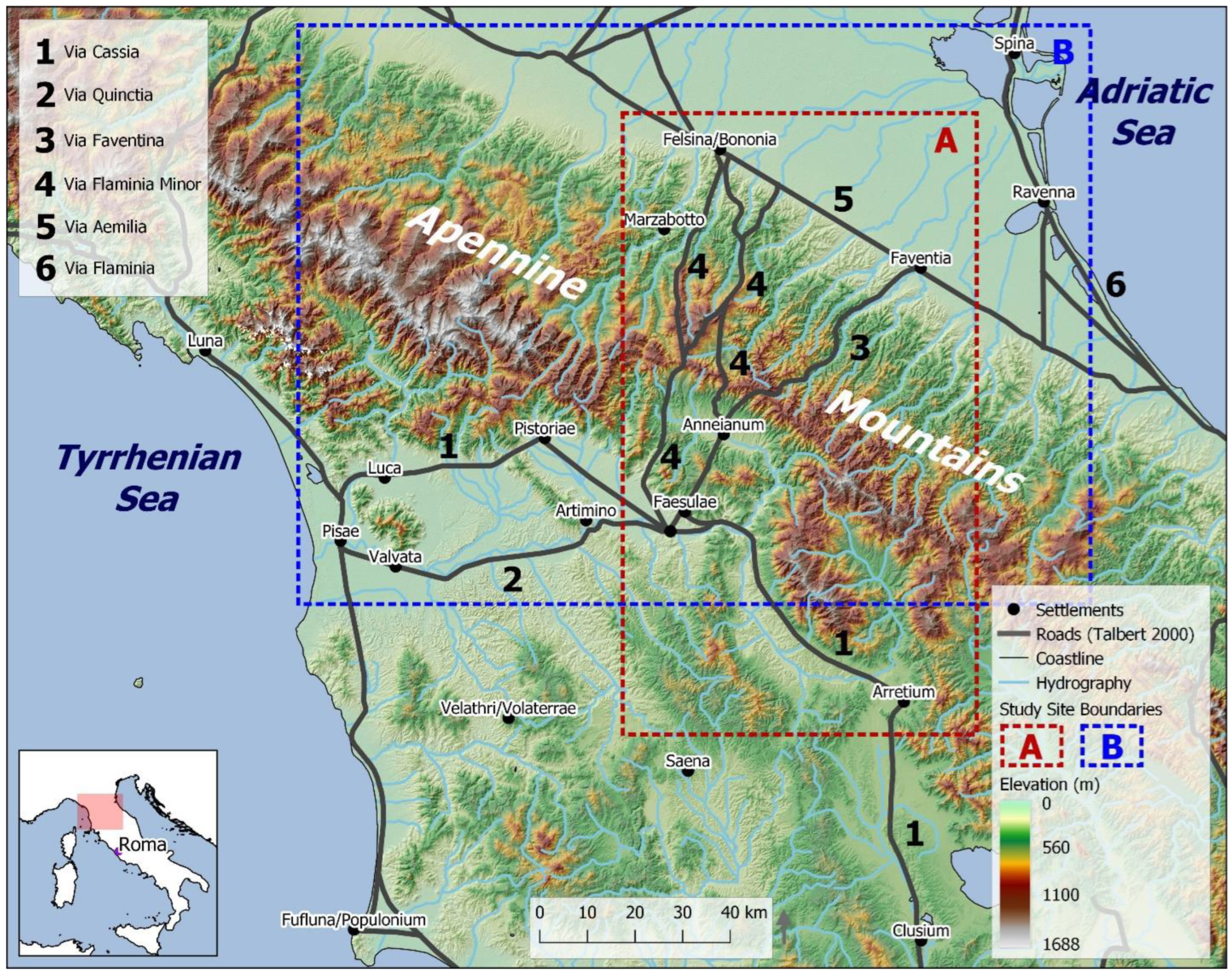
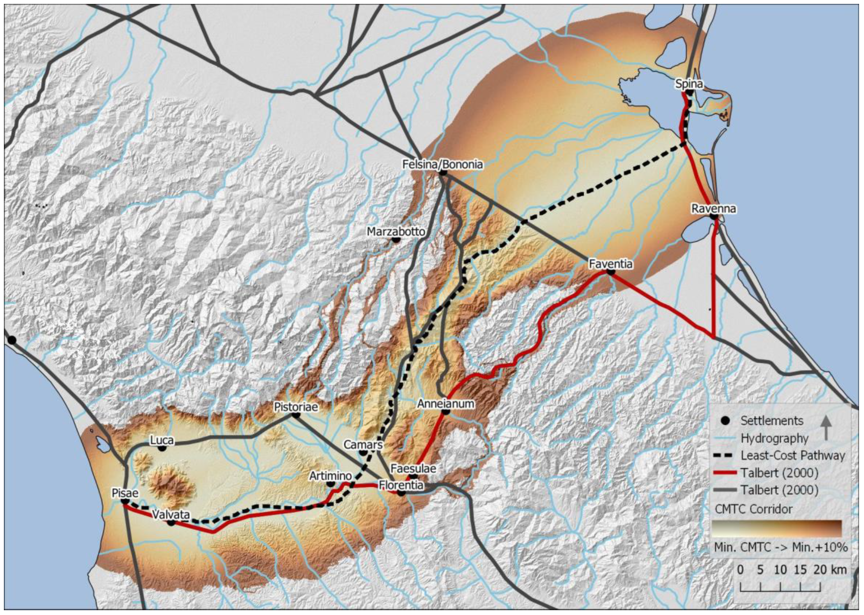
The study area for our research is northern Etruria, a region located in the northern part of ancient Italy. This region has two overlapping study sites roughly outlined by bounding boxes in Figure 1 and identified by the names of the main roads under investigation: Via Flaminia Minor (Site A) and Via Etrusca del Ferro (Site B). Northern Etruria was framed by the Apennine Mountains to the north and east, the Tyrrhenian Sea to the west, and southern Etruria and Umbria to the south (Figure 1). In this region of about 11,500 km², terrain elevation ranged from sea level to about 1688 m in the Apennine Mountains, and the Arno River (ancient name Arnus) was the largest water body and was most commonly used for water transportation in the region.

According to ancient sources such as the geographer Pseudo-Skylax, the Etruscans initially built roads in northern Etruria as far back as the fifth century BCE [19]. Several locations in southern Etruria evidence the sophistication of Etruscan road building [20]. As Rome colonized Italy from the third to the first century BCE, the Romans built new roads in the region and also reconstructed and took over the maintenance of some Etruscan-built roads [3,21]. (Re)constructed Roman roads followed the guidelines and standards laid down in the Twelve Tables, which stipulated that roads must be paved, layered, and measure eight Roman feet wide on a straightway and 16 Roman feet wide on bended sections to enable side-by-side passage of two wagons [3]. Over the years, many scholars such as Riparbelli [13] and Talbert [6] have mapped northern Etruria roads, yielding conflicting results in some areas.

2.1. Site A: Via Flaminia Minor

In one of his writings in the first century BCE, Livy (39.2.5-7) credited the Romans for building the Via Flaminia Minor to connect Bononia and Arretium, following their military victories over the Ligurian Apuani in 187 BCE. This was the second Roman road constructed in northern Etruria, and the first in the eastern part of the Arno Valley, despite the Romans having been active in the region since at least the third century [22]. 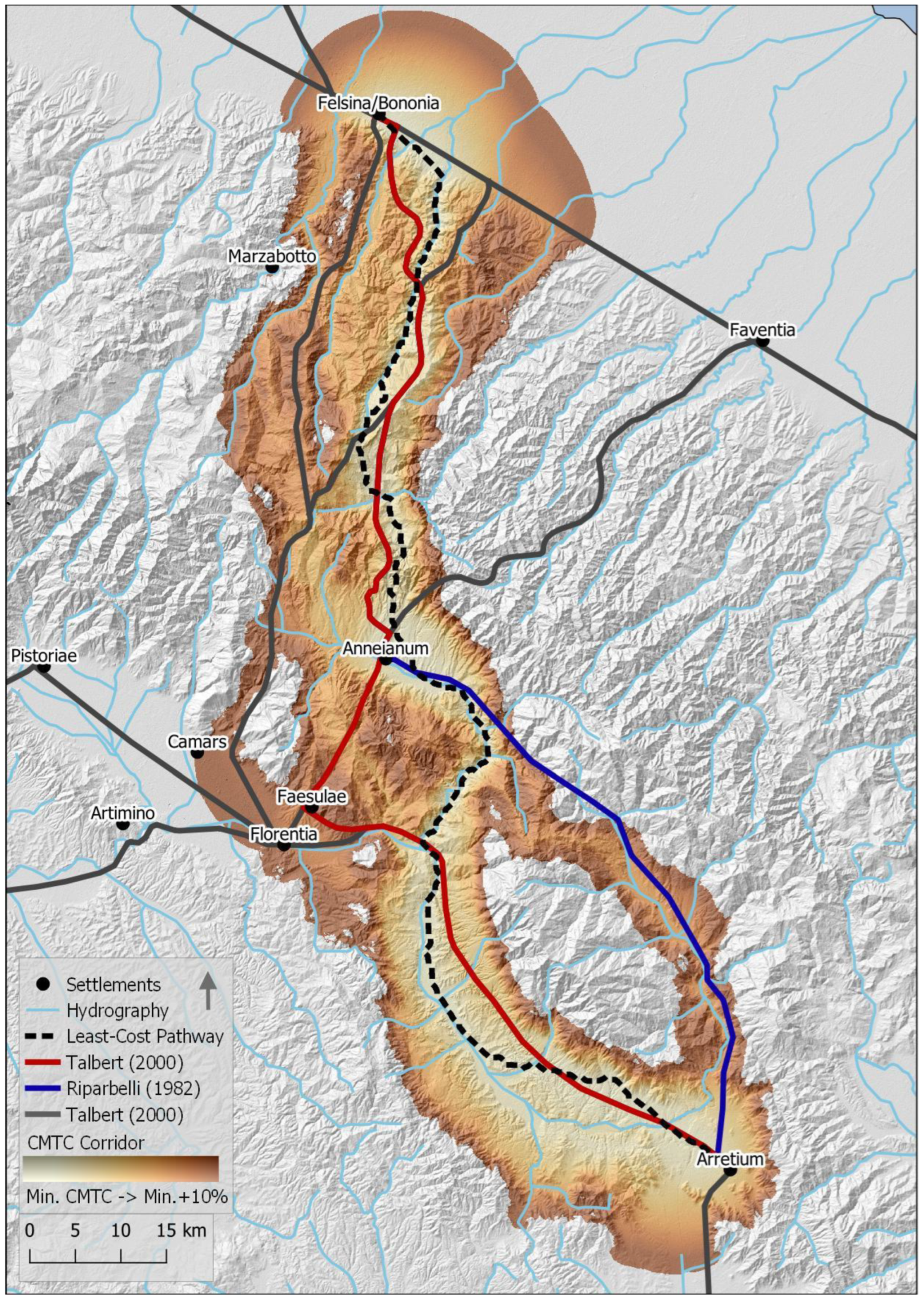Alfieri [23] was first to identify the northern segment of the Via Flaminia Minor, starting at Bononia and going south roughly along the Idex River and close to the Etruscan city of Marzabotto. Other scholars have extended this segment to reach Arretium, albeit along different routes. Riparbelli [13], for example, suggested that the southern portion of the Via Flaminia Minor went via Anneianum and along the headwaters of the Arno River to Arretium. Talbert [6] conversely drew several routes that connected Alfieri’s segment to the cities of Faesulae and Florentia before following the Via Cassia along the Arno River to Arretium. If we accept the logic that military roads actively avoided existing non-Roman population centers, then Riparbelli’s route seems more plausible but the establishment and importance of Florentia to the Romans in the 1st century BCE may alternatively indicate that the road was much closer to Faesulae as mapped by Talbert.

2.2. Site B: Via Etrusca del Ferro

Pseudo-Skylax’s report, written around the mid-fourth century BCE, states that the Via Etrusca del Ferro was built before the Romans arrived in northern Etruria [19]. Pointing out that this created a transportation link connecting the western and eastern coastal cities of Pisae and Spina, Pseudo-Skylax claimed that the road enabled people to travel across the Italian peninsula between the two settlements in just three days on average [19]. This timeframe seems to underestimate the straight-line distance of nearly 175 km or the distance along Talbert’s [6] route of approximately 255 km between the cities (see Section 5). Although questionable by ancient standards, Pseudo-Skylax’s claim is tempting to accept as merely an implication that the Via Etrusca del Ferro was well-constructed and relatively efficient to travel.

Many scholars have put forward different views about the exact route for Via Etrusca del Ferro. Rauty [24] described it as an Etruscan road that passed through modern Pistoia before crossing the Apennines and connecting to Bononia. Mosca [25,26] suggested that the Via Quinctia and Via Faventina (Figure 1) built by the Romans in the second and first centuries BCE were basically reconstructions of an original Etruscan road that corresponds to the Via Etrusca del Ferro. Other scholars have also argued that the original Etruscan road was located further north in the Arno Valley, along the later Roman Via Cassia [13,21]. Still, some scholars believe that physical evidence of Etruscan-built roads found near Luca are the remnants of the Via Etrusca del Ferro [27].

3. Ancient Road Mapping Methods and Materials

Encouraged by the spatial turns in archaeology and history, and the computational power of geospatial technologies, many studies about the past are employing GIS together with archaeological approaches to map and understand how road networks shaped human mobility patterns [12,28,29,30]. 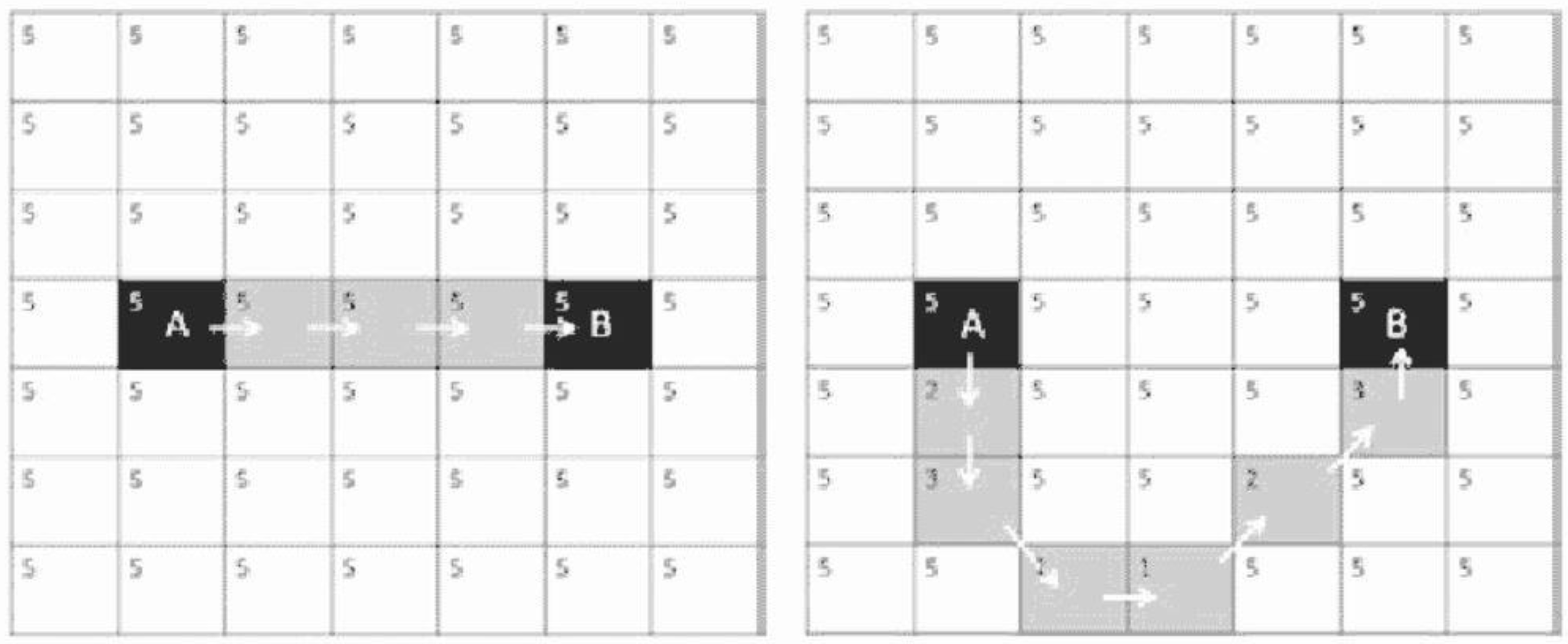Least-cost path analysis (LCPA) is the most widely used GIS technique for determining optimal pathways between points (e.g., cities) on a cost surface created at point of origin based on one or more criteria [16,17,18,28,31,32]. LCPA pathways are drawn starting at destination (i.e., target) and ending at origin (i.e., source) points, which makes identifying these points based on characteristics such as functions, roles, and pull or push factors that cause unequal ‘two-way’ movement between settlements an important step (Figure 2) [32]. Criteria such as landcover, slope gradient, means of transport (e.g., animal-drawn cart), and physical barriers (e.g., steep cliffs and non-navigable waters) can be weighted to reflect their perceived importance or levels of influence on human movements or other phenomena.

LCPA has concerns of its own related to input data, cost-surface criteria, and the output [30]. Incomplete data for modeling movement between sites or representing ancient phenomena through recent geospatial data all present challenges in creating reliable feasible paths [32]. The same is true for identifying complete sets and assigning appropriate weights to criteria for generating cost-surfaces. LCPA pathways are typically discrete, giving the impression of precise GIS modeling, a problem that can be solved by generating fuzzy paths where pixel values denote relative likelihood of a given route passing through that pixel or geospatial location. We implement this solution through the conditional minimum transit cost (CMTC) technique, developed for ecology, creating least-cost travel corridors that convey mapping uncertainty, which degrades with distance from the optimal path [33].

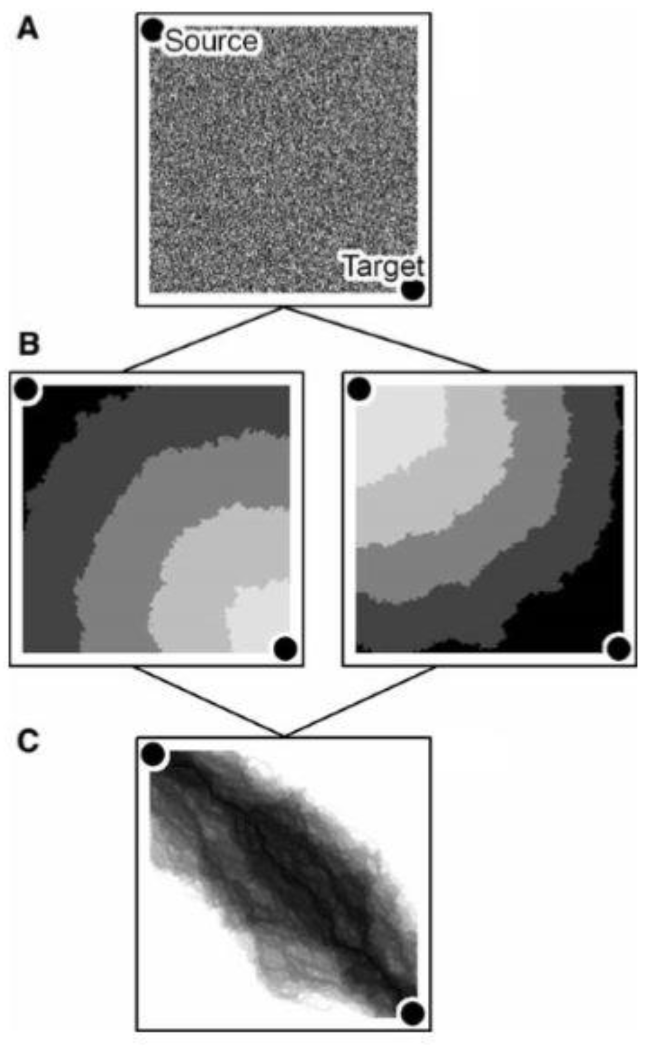
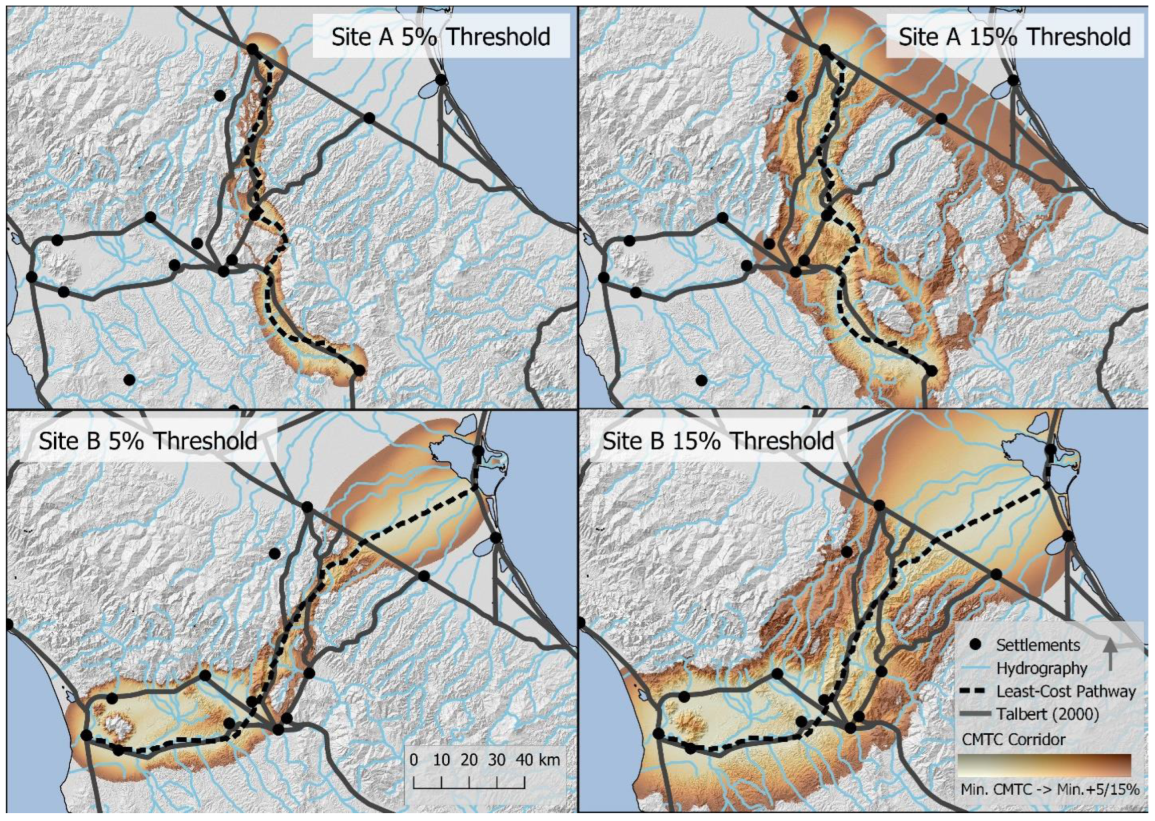
Citing Forman [34], Pinto and Keitt [33] treat corridors as thin land areas that differ from their surroundings in some specific way(s) (e.g., ease of travel). The corridors are created in two related steps [33]. First, cost surfaces are generated radiating from both source and target points, based on the energy “cost” expended to traverse landscapes and water features, and combined into a single surface by averaging (Figure 3). Second, pixel values ranging from the averaged minimum travel cost to the averaged minimum travel cost plus 10% of that least value are identified to highlight the travel corridor. Although 10% is an arbitrary figure chosen by Pinto and Keitt, we also found this threshold optimal for our study. The threshold helped us to create travel corridors that wholly contained archaeologically-mapped roads of interest. Threshold values above 10% generated wider corridors at odds with Forman’s definition, while values below 10% created thin regions that excluded important roads (Figure 4).

3.1. Geospatial Datasets

Study data are divisible into vector (i.e., cities, towns, roads, coastlines, and hydrography), raster (i.e., DEM) and non-geospatial (e.g., road, river, and settlement names). Most of these data (i.e., vector and attribute) are digitized versions of analog map layers available in the Barrington Atlas of the Greek and Roman World but were sourced from these public-facing repositories: Digital Atlas of Roman and Medieval Civilizations (DARMC) (https://darmc.harvard.edu/ (accessed on 5 April 2020)), Ancient World Mapping Center (AWMC) (http://awmc.unc.edu/wordpress (accessed on 5 April 2020)), and Pleiades Project (https://pleiades.stoa.org/places (accessed on 5 April 2020)). The 30 m DEM accessed from AWMC is NASA’s product from 2012 Shuttle Radar Topography Mission (STRM) and clearly not ancient or bare earth data. These data are the basis for generating important slope and relief maps, elevation profiles, and other visualizations of terrain attributes. It should ideally be adjusted to mirror ancient topography but this has not been achieved because considerable topographic changes occurred in relatively small areas around metropolitan areas such as Florence and Arezzo and only more substantially on the western coast of the Arno Valley near port of Pisa [35,36]. Although the correction of DEMs is preferred, the use of modern elevation models in studies such as these has long been accepted, especially in areas where terrain surface corrections are difficult to determine [32]. Modern DEMs may not faithfully represent ancient terrain in regions that have undergone considerable topographic changes (e.g., due to earthquakes), thereby affecting the quality of results of geospatial analytical exercises involving terrain modeling. Here, we assume that any topographic changes or nuances introduced by terrain features such as vegetation and urban developments are barely noticeable on the relatively low-resolution DEM and have little or negligible impact at our study site levels.

3.2. GIS-Based Tools and Techniques

Initial steps for GIS-based ancient road mapping included identifying source and target points and appropriate criteria for constructing human movement cost surfaces. Without strong rationale (e.g., relative sense of place) to distinguish between settlement points, we randomly selected Arretium and Spina as source points for LCPA of Via Flaminia Minor and Via Etrusca del Ferro. Cities at the ends of these highways served as origin points in making CMTC cost surfaces. 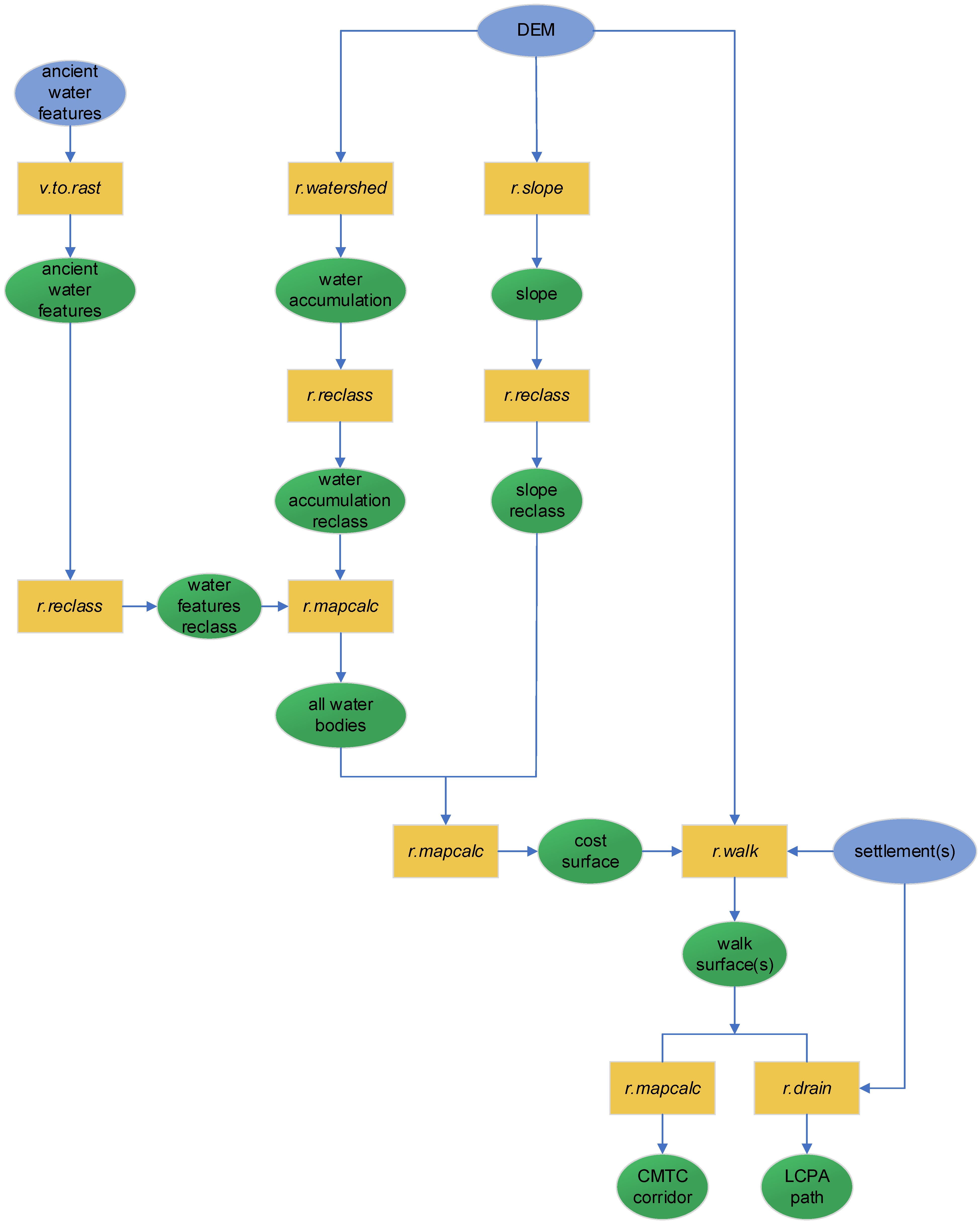Figure 5 shows that criteria related to terrain elevation, terrain slope, hydrography (i.e., water bodies), and mode of transport were used to model CMTC corridors and LCPA paths. The unavailability of reliable data led us to leave out possible criteria such as landcover, landscape visibility, and attractiveness of cultural centers for future work [37]. For example, landcover data for ancient features such as forests were not accessible, and although long-range landscape visibility can avert ambushes or expand scenic areas, we were uncertain about the importance of this factor in routing Via Flaminia Minor and Via Etrusca del Ferro, even though it was considered in modeling other Roman roads by Verhagen and Jeneson [16]. Incomplete cultural data encouraged us to focus on physical efficiencies of routes connecting settlements explicitly mentioned in ancient written sources. This allowed us to speculate on the cultural significance required to detour routes from physically optimal pathways to those settlements between explicitly stated locations.

The tenets of open-source software [38] persuaded us to opt for two cost-free but advanced and user-friendly open GIS: Quantum GIS (QGIS) and GRASS GIS. We were able to use these software seamlessly together to organize, integrate, explore, and make sense of complex geospatial information. Figure 5 depicts our GIS-based geoprocessing workflow that identifies GRASS GIS functions and geospatial data used to complete LCPA and CMTC modeling. An r.slope function was first run on the DEM, generating a terrain slope map useful to identify where people could efficiently walk across the study area. Drawing on previous studies [39,40], we allocated prohibitive travel costs that increased with terrain slope such that feasible paths would avoid gradients (i.e., >15% or 9°) viewed to be challenging for wheeled vehicles. A 100-point scale was used to reclassify and transform all datasets to the same unit costs to facilitate integrative analysis. This included the slope map, which was reclassified based on the perceived difficulty different gradients would present to pedestrian and wheeled transport.

To ensure that LCPA paths did not follow less demanding slopes in areas such as valleys where water typically accumulates, we executed r.watershed on the DEM, creating a drainage flow accumulation raster map of streams, rivers, and precipitation runoff, which were all considered in creating travel cost surfaces. One important aspect of this map is that it highlighted areas with little or no water accumulation where roads could be built without risk of being washed away. We also prohibited modeling human movement across large hydrography by rasterizing and assigning high pixel values to ponds, lakes, and seas. Using r.mapcalc to combine these rasterized and reclassified water features and reclassified water accumulation helped us to create a comprehensive water bodies dataset. The resulting layer was then combined with reclassified slope gradients using r.mapcalc to create a cost surface.

Although it is conceivable that modes of transport such as horse-riding and wagons were used in northern Etruria, we assumed that even travel with those vehicles were typically accompanied by people principally walking between locations. Thus, we implemented r.walk on a combination of cost surface, DEM, and settlement datasets. The function “computes anisotropic cumulative cost of moving between different geographic locations on an input elevation raster map whose cell category values represent elevation combined with an input raster map layer whose cell values represent friction cost” (https://grass.osgeo.org/grass78/manuals/r.walk.html (accessed on 15 September 2020)). Put differently, r.walk applies Naismith’s Rule about people’s rate of walking on various terrain slopes on the DEM and a friction surface considering the other travel costs [41,42] to produce walk surfaces or anisotropic cost surfaces. Walk surfaces originating at one (i.e., for LCPA) and two endpoints (i.e., for CMTC modeling) of Via Flaminia Minor and Via Etrusca del Ferro were input datasets to r.drain and r.mapcalc functions. The former was used to draw the least-cost path beginning at target point going over cost surface pixels with lowest travel cost all the way to source point. The latter was first used to average walk surfaces originating at both highway endpoints and second highlight areas with minimum average cost outward to areas up to minimum average cost plus 10%.

4. Road Map Comparison Criteria and Methods

There are many criteria available to describe and measure the types of inconsistencies between linear geospatial features such as roads, trails, and streams. A question that immediately comes to mind is how many criteria and which ones are essential to gain detailed insight and take appropriate actions for conflicts between ancient road maps. The specific answer is context-dependent and might be related to map comparison goals and purpose, for example. Here, our interest is broadly driven by the need to reveal potential geospatial differences between several views of ancient features, discourage uncritical use of single map perspectives where ground-truth is not comprehensive, encourage consideration of available possibilities about ancient communities, and motivate evaluations that produce knowledge about possible impacts of conflicting map views on projects.

As maps are visual displays, visual methods are naturally part and parcel of juxtapositions of these products. These methods engage our visual senses, allowing us to ‘see’ map inconsistencies sometimes much faster than computational techniques [43,44]. In previous studies, they brought to light perceptible differences between equivalent roads mapped by different experts [17], various tools and techniques [31], and similar methods [16]. Other scholars have superimposed ancient roads on different geospatial features to visually evaluate (mis)matches and ascertain the relative quality of their routes. This geospatial overlay technique showed that ancient roads in two separate study areas fell within at least 1 km of most archaeological sites and matched nearly a quarter of modern roads buffered by 500 m [18,45]. Together, the studies discussed here employed length, sinuosity, travel time along the features and proximity to other features of interest as linear feature comparison criteria. Verhagen et al. [37] also suggest deviation from the straight-line path between points as a criterion that could provide an additional perspective for improved understanding of linear feature differences.

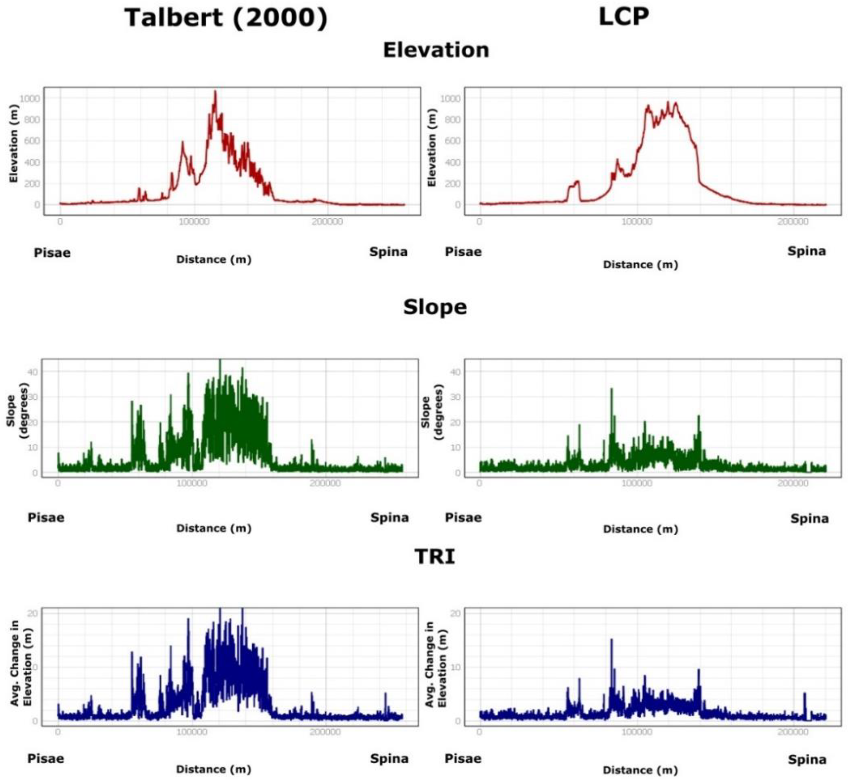
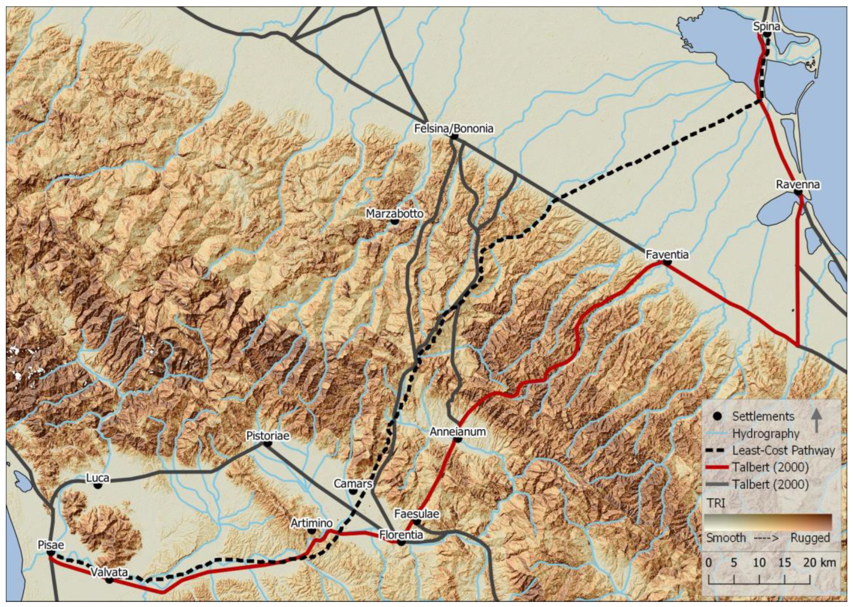
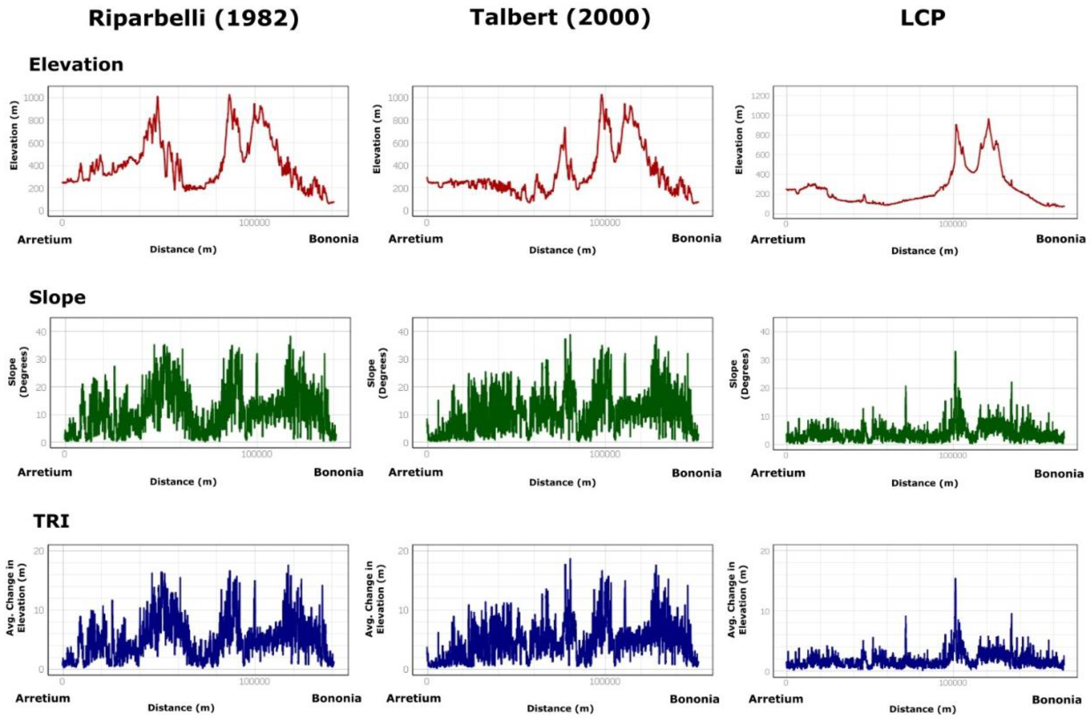
Another takeaway from the above studies is that blending qualitative and quantitative criteria and methods offers an ideal approach to display, uncover, analyze and assess road map differences. We adopt some of the criteria and incorporate others to compile a relevant and robust set to achieve our goals, and provide a basis on which others can identify and adapt practical measures for their applications. We employ visual skills to qualitatively measure route (1) lengths, (2) sinuosities, and (3) locations in study sites, CMTC corridors, terrain elevation surfaces, and terrain roughness index (TRI) surfaces. TRI surfaces enable visualizing and sense-making about the complexity of the terrain upon which ancient roads were likely set. The surfaces are determined from the elevations of individual pixels and their contiguous neighbors and offer a quantitative means for assessing the degree of terrain ruggedness. Low pixel values describe level to slightly rugged terrain generally easy to navigate, and therefore we assumed these areas were preferred for road construction [46]. High pixel values imply highly or extremely rugged terrain generally difficult to traverse (ibid). Thus, our qualitative and quantitative criteria overlap slightly, and the latter are related to (1) route lengths; (2) route separations; and (3) the complexity of the terrain on which different routes were embedded as determined by minimum, maximum, and mean values plus profiles of terrain elevation, slope, and TRI. We use Cole and King’s [47] detour index (DI) to measure the degrees of possible route separations. This index is calculated by dividing straight-line and actual path distances between two points, giving values that range from 0 to 1 and indicate greater and smaller deviations from the straight line, respectively [47].

5. Results and Analysis

5.1. Site A: Via Flaminia Minor

Many researchers agree with Livy (39.2.5-7) that the Via Flaminia Minor was established to connect communities in Arretium and Bononia. Taking Livy as a credible source, we know the exact starting and ending ‘points’ of this highway. Based on physical evidence, researchers also have confidence in the courses of the northern segments of this highway that ran roughly between Anneianum and Bononia [23] (Figure 6). What remains largely unknown are the whereabouts of the southern segment(s) currently informed by mixed and inconclusive ideas. Both Riparbelli [13] and Talbert [6] proposed segments that start at Arretium but proceed along different paths to Anneianum and Faesulae, respectively, although Talbert’s [6] route is generally the more widely accepted route [48]. Because these scholars separately sought to map only the southern piece of Via Flaminia Minor given widely accepted information about the northern portion, there are essentially many complete versions of this highway matching in northern but not southern portions.

It seems fair to juxtapose the full-length variants of Via Flaminia Minor suggested by Riparbelli [13] and Talbert [6] against the GIS-modeled least-cost path (LCP) which, based on Livy, has Arretium and Bononia as endpoints. We digitized the southern section of Riparbelli’s version into our GIS from a PDF copy of Riparbelli [13] and downloaded Talbert’s [6] version from the DARMC as a GIS-ready file. We describe Riparbelli’s full version of the Via Flaminia Minor as one that begins at Arretium and goes through Anneianum before heading north along one of the widely accepted and, for analytical purposes, shortest routes to Bononia (Figure 6). Although the starting point for Talbert’s route is also Arretium, this road initially goes to Faesulae before passing through Anneianum and following the same road segment to Bononia as Riparbelli.

In examining Figure 6 and Figure 7, we learn that the southern segments of the Via Flaminia Minor put forward by Riparbelli and Talbert do not coincide or cross paths anywhere along their lengths of 74 km (i.e., Arretium to Anneianum) and 85 km (i.e., Arretium to Faesulae and then Anneianum), respectively. These segments generally fall within the same CMTC corridor and appear to be delineated on terrains with similar elevations and roughness. A portion of Riparbelli’s route falls outside the CMTC corridor and about two-thirds of this highway appears to closely follow the Arno River feature near its headwaters before intersecting another water body close to Anneianum. Talbert’s route also intersects the Arno River, although near Arretium, and cuts across several tributaries, much like Riparbelli’s, indicating that the southern section of the Via Flaminia Minor likely had many bridges that, for lack of information, are not represented along either route.

Although Talbert’s route takes a somewhat sharp turn as it veers west away from the LCP, both archaeological roads show overall gradual changes in direction. The limited degree of sinuosity or meandering appears to be in line with Roman standards that encouraged designing and constructing straight roads which, as a result, sometimes went through complex (e.g., very steep) terrain [3]. Taking a closer look at archaeological versus GIS roads (i.e., LCP’s) reveals that Talbert’s route generally agrees with the LCP, while Riparbelli’s is relatively close to this path only near Anneianum. Digging into the specific causes of these (dis)agreements is important but outside of the scope of this study. That said, we suspect that pictures developed here are explainable by factors such as (1) inconsistent sources of foundational information, (2) different assumptions, biases, or levels of imprecision built into archaeological and GIS mapping processes, and (3) criteria considered relevant and then weighted, combined, and applied in various ways in different mapping exercises.

Looking at route lengths, it is clear that the GIS LCP is longer than archaeologically produced variants of Via Flaminia Minor by distances of 14.0 km and 25.2 km, which may be viewed as considerable (

Table 1. Summary of quantitative differences between variants of the Via Flaminia Minor.

Comparison Measure			Riparbelli (1982) ®	Talbert (2000) (T)	GIS LCP	R-T	R-LCP	T-LCP
Length (km)			141.2	152.4	166.4	−11.2	−25.2	−14
DI (straight-line: 122.3 km)			0.87	0.8	0.73	0.07	0.14	0.07
Terrain Landscape Complexity	Elevation (m)	min	62.3	62.3	66.8	0	−4.5	−4.5
		max	1028.7	1028.7	967.5	0	61.2	61.2
		mean	412.6	331.6	259.5	81	153.1	72.1
		relief	966.4	966.4	900.7	0	65.7	65.7
	Slope (deg/%)	min	0/0	0/0	0/0	0/0	0/0	0/0
		max	38.4/79.2	38.9/80.8	33.1/65.3	−0.5/−1.6	5.3/13.9	5.8/15.5
		mean	11.4/20.6	10.9/19.6	4.1/7.1	0.5/1.0	7.3/13.5	6.8/12.5
	TRI	min	0.01	0.02	0.03	−0.01	−0.02	−0.01
		max	17.63	18.67	15.44	−1.04	2.19	3.23
		mean	4.89	4.7	1.81	0.19	3.08	2.89

). Despite being initially close to the LCP, Talbert’s route is ultimately longer than Riparbelli’s and its lower DI value (i.e., 0.80) implies that it is not the more direct link between Arretium and Bononia. A journey along each archaeological route would take individuals through high relief (i.e., 966.4 m) terrain, although those on Riparbelli’s would experience overall higher mean elevation due to their closer proximity to the foot of the Apennine Mountains. Mean slopes of archaeological versions of Via Flaminia Minor are close to 15–20% grades typical and acceptable for Roman roads built in hilly areas but less than half (i.e., 7.1%) of these figures and more manageable for LCP [49]. The maximum slopes of 65.3–80.8% seem unrealistically too high, though. This could be the result of incorporating terrain feature heights into the SAR-derived DEM or an artifact of DEM resolution, which can increase the grade by up to an incredible 420% when improved from 90 m to 3 m [50].

The profiles in Figure 8 offer a strong means to further explore and comprehend how the physiographic attributes of elevation, slope, and ruggedness varied along each version of the Via Flaminia Minor. Taken together, these cross-sectional views illustrate that people travelling between Arretium and Bononia would repeatedly go up and down in altitude through generally rough terrain characterized by diverse slopes ranging from flat (i.e., 0°) to very steep (i.e., 33.1–38.9° or 65.3–80.8%). Going from Arretium (altitude 250 m) to Bononia (altitude 72 m), the individuals would reach an altitude of about 1000 m along Riparbelli’s and Talbert’s routes after about 49 km and 97 km, respectively, which suggests that there is a quicker and likely more challenging elevation gain along the former. Zeroing in on the elevation profiles, it appears that all three routes go over many hills including at least three with peak altitudes greater than 600 m, which could be demanding depending on whether one is on foot, horseback, animal-drawn cart, or using some other mode of transport. The elevation profiles also reflect fewer and relatively less striking random fluctuations than those for slope and TRI, which appear identical or strongly related. All three types of profiles seem to point to strong similarities between the intricacies of the terrain landscapes of Talbert’s route and LCP.

5.2. Site B: Via Etrusca del Ferro

Of the several ideas concerning the location of the Via Etrusca del Ferro, we are aware of only two that are conveniently available in map form, that is, Talbert’s [6] (citing Mosca [25,26]) and our LCP. Although Rauty’s [24] text-based perspective is valuable, it seems appropriate and reasonable to compare only map-based forms of this highway. Doing so enables us to perform more reliable geospatial visualization, analysis, and interpretation tasks and uncover subtle differences between equivalent routes. With respect to Figure 9, it can be said that beginning at Pisae, Talbert’s road proceeds eastward through seven notable settlements (i.e., Valvata, Artimino, Florentia, Faesulae, Anneianum, Faventia, and Ravenna) before reaching Spina. In contrast, LCP goes through Valvata and comes close to the Etruscan settlements of Artimino and Camars before going halfway between Bononia and Faventia to reach Spina. There is initial agreement between LCP and Talbert’s road between Pisae and Artimino but after that the two routes are fairly distant from each other except near Spina.

Although we do not endorse or refute either map-based view discussed above, Mosca’s [25,26] suggestion that Roman roads represented in the Arno Valley and Apennine Mountains replaced an older Etruscan highway lends credence to Talbert’s route, which, as can be deduced from superimposing Figure 1 and Figure 9, is essentially an aggregation of several Roman roads connecting various settlements. Talbert’s route is clearly longer than LCP and barely makes it inside the CMTC corridor roughly between Anneianum and Faventia. Both routes exhibit overall similar degrees of sinuosity for most of their lengths and occur in low (e.g., near Pisae and in the Po River Valley) and high-altitude areas and in flat and rolling terrains. The routes differ in their relationships with regional water bodies and possible sources of drinking water for travelers in that Talbert’s route follows the Arno River while LCP mostly cuts across its tributaries.

As can be seen in

Table 2. Summary of quantitative differences between versions of the Via Etrusca del Ferro.

Comparison Measure			Talbert (2000) (T)	GIS LCP	T-LCP
Length (km)			255.1	220.7	34.4
DI (straight-line: 174.8 km)			0.69	0.79	0.1
Terrain Landscape Complexity	Elevation (m)	min	−8.9	−6	−2.9
		max	987.4	967.5	19.9
		mean	129.4	183.3	−53.9
		relief	996.3	973.5	22.8
	Slope (deg/%)	min	0/0	0/0	0/0
		max	43.3/94.2	33.4/65.9	9.9/28.3
		mean	6.3/11.5	2.9/5.2	3.4/6.3
	TRI	min	0	0	0
		max	21.99	15.24	6.75
		mean	2.81	1.41	1.4

, each route is characterized by negative minimum elevation values, implying that a portion of each road is below mean sea level or possibly under water. GIS analysis located these lowest altitude areas near Spina. Upon zooming into the vicinity of Spina (Figure 10), we see some interesting but expected mismatches between the GIS data layers gathered from several sources that vary in map scale and quality, including currency and locational accuracy. In essence, Figure 10 brings to light some of the issues that can be encountered when ancient (e.g., coastline) and modern (e.g., DEM) datasets are combined and visualized together [51]. A common way to fix misaligned geospatial phenomena within GIS is to adjust one dataset to conform to the other considered true or more reliable. This study intentionally did not attempt to implement this solution because we considered the level of inconsistency minor in mapping the ancient world at a scale of 1:500,000 or 1:1,000,000 [6,7].

Focusing on the horizontal axes of the profiles in Figure 11 we note that Talbert’s route stretches between Pisae and Spina over a longer distance than the LCP. The lengths of the two routes differ by 34.4 km (~21.2 mi), which seems substantial by any measure (Table 2). At the same time, a smaller difference would probably be just that and not necessarily point to similarities between the criteria, tools (e.g., input data or supporting evidence), approaches, or other elements which can influence the nature of the outputs, including overall quality of GIS and archaeological mapping exercises. The difference between DI values of 0.10 (Table 2) seems to confirm the scale-dependent map perspectives from Figure 9 and Figure 12 that Talbert’s route deviates considerably from the LCP. Whether one travels efficiently or not along either road is determined by several factors such as terrain elevation, slope, and roughness. Higher elevations (e.g., +1500 m), for example, require getting used to failure of which one can experience altitude sickness (Fleetwood 2019). Talbert’s route peaks at an altitude of 987.4 m, which is 19.9 m above the LCP summit (altitude 967.5 m) (Table 2) and the two peaks of the two routes are reached after about 116 km and 91 km from Pisae, respectively, indicating a steadier ascend that is good for height acclimation along the former.

Moving between Pisae and Spina, one would navigate through generally gentle terrain in the Arno River and Po River valleys at the beginning and end of that journey, respectively, but experience rough terrain in the Apennine Mountains between the two cities. Based on terrain relief (Table 2) and elevation profiles (Figure 11), one would also experience a higher overall elevation gain/loss along Talbert’s route, which also exhibits higher amplitudes for slope and TRI variables than the LCP. The TRI values and profiles also suggest overall similar levels of terrain complexity at the beginning and end sections of all versions of the Via Etrusca del Ferro but the middle portions appear to be more rugged and steep along Talbert’s route. As was the case in the previous study site, the mean slopes of 11.5% and 5.2% for Talbert’s route and the LCP, respectively, fall within acceptable standards for ancient Roman roads.

6. Conclusions

The process of creating quality maps of ancient settlements can expend quite a lot of time, effort, money, and other resources but is essential to tell elaborate and meaningful spatial stories about how past communities might have existed and possibly influenced the trajectory of later groups [5]. A crucial part of our study involved differentiating between map-based perspectives of similar ancient road routes in northern Etruria. These juxtapositions did not and were intentionally not intended to identify any mapping products, professionals, or methods that might be considered better (e.g., more trustable) than their counterparts. Rather, they were conceived and proved useful for highlighting the types and degrees of possible differences between maps of similar geographic phenomena made by different experts through GIS and archaeological approaches.

Map (dis)agreements were determined, understood, and explained based on a combination of qualitative and quantitative methods and specially compiled comparison criteria. As expected, the qualitative method was more efficient at detecting nuanced differences and similarities between map content but suffers from limitations of human subjectivity such that analysts with different proficiencies in visual analysis and interpretation have great potential to reach different findings and conclusions. Thus, qualitative methods of comparing maps should ideally be applied in conjunction with their quantitative counterparts that can greatly reduce the element of subjectivity while simultaneously adding important reproducibility and credibility factors.

The study findings underscored and reiterated that both traditional and modern (e.g., GIS-based) processes of mapping the past incorporate inexactitudes influenced by data, human, technological, and methodological factors. The findings exposed substantial differences between equivalent roads mapped using similar archaeological methods by different experts, and between these roads and those produced through GIS modeling. The differences were evident in terms of road lengths, sinuosity, and geographic locations as well as levels of complexity of the landscapes the roads went through as defined by subtle variations in terrain elevation, slope, and ruggedness. Their magnitudes ranged from 11.2–34.4 km in road length, 0–65.7 m in road relief, 1.0–13.5% in mean road grade, 0.07–0.79 in DI and 0.19–3.08 for average TRI values. Surprisingly, GIS and archaeologically produced roads matched only where they originated, intersected, or terminated and were sometimes apart by as much as 30 km in perpendicular distance.

The types and magnitudes of inconsistencies uncovered in this study bring up valid concerns about the quality of different mapping processes and associated products. Assessing these concerns is valuable toward understanding inextricably linked levels of quality of the conclusions, decisions, or actions that may be taken based on the content of different maps. Where ground-truth informed assessments cannot be reliably performed, the more the number of conflicting or congruous ideas or insights the better, especially where investigators are trying to dig deeper into the lives and connections between ancient communities. It is thus imperative to explicitly acknowledge and maintain all usable perspectives in geospatial databases plus visualization and analysis processes regardless of the degrees of disagreement. This may be challenging, particularly in applications that have traditionally sought to construct and propagate a single authoritative understanding of certain aspects of the real-world. It is, of course, not to say that there are no applications which deal with a single and perhaps widely accepted view of reality.

The methods and materials used to create maps examined in this study are strong and limited at identifying the real routes used in the ancient world, and it is important to identify and incorporate their best aspects in studies about the ancient world. For instance, the content of GIS maps is often well packaged and looks aesthetically pleasing, giving an aura of accuracy and authenticity, but these products may not necessarily be better than those created through archaeological or other mapping techniques. As noted in other studies [30], contemporary GIS datasets such as DEMs and landuse-landcover maps may need to be antiqued before being used to map ancient settlements, especially those in geographic regions believed to have undergone significant landscape changes over time. The cost of a GIS solution has also been cited as a factor that discourages implementing this interdisciplinary technology, but it is worth repeating here that all geospatial tasks in this study were completed satisfactorily using open-source GIS software available free of charge, illustrating that their power is just as strong as that of commercial proprietary products.

There are many ways to improve and extend this study and these include those broadly concerned with data, analytical, and assessment issues. The first is about conducting on-site surveys in search of more physical evidence, perhaps through drone-supported surveying or ground penetrating radar, or to develop a complete LiDAR dataset for the area. That evidence would support more effective assessments of ancient road maps. The second is related to LCPA and focused on creating better cost surfaces that incorporate additional or appropriately weighted criteria (e.g., historical landcover). A third approach might apply higher resolution and temporally-corrected DEMs to acquire a good picture of ancient terrain landscapes and where different roads might have cut through. Finally, it would be interesting to apply the linear referencing technique to measure the average separation between corresponding roads deduced or modeled through different approaches.

References

1. Newhard, J.M.L.; Levine, N.S.; Phebus, A.D. The development of integrated terrestrial pathways in the Argo-Saronic region, Greece. Cartogr. Geogr. Inf. Sci. 2014, 41, 379–390. [Google Scholar] [CrossRef]
2. Rippon, S. Historic landscape character and sense of place. Landsc. Res. 2013, 38, 179–202. [Google Scholar] [CrossRef]
3. Laurence, R. The Roads of Roman Italy: Mobility and Cultural Change; Routledge: London, UK, 1999. [Google Scholar]
4. Bodenhamer, D.J.; Corrigan, J.; Harris, T.M. Deep Maps and Spatial Narratives. Bloomington; Indiana University Press: Bloomington, IN, USA, 2015. [Google Scholar]
5. Martinez-Davila, R.L.; Hodza, P.; Kapadia MPerrone, S.T.; Holscher, C.; Schinazi, V.R. Telling Stories: Historical Narratives in Virtual Reality. In The Routledge Handbook of Digital Medieval Literature; Boyle, J., Burgess, H., Eds.; Taylor & Francis Ltd.: Oxfordshire, UK, 2017; pp. 107–130. [Google Scholar]
6. Talbert, R.J.A. Barrington Atlas of the Greek and Roman World; Princeton University Press: Princeton, NJ, USA, 2000. [Google Scholar]
7. Talbert, R.J.A. Challenges of Mapping the Classical World; Routledge: London, UK, 2019. [Google Scholar]
8. Conolly, L.; Lake, M. Geographical Information Systems in Archaeology; Cambridge University Press: Cambridge, UK, 2006. [Google Scholar]
9. Cope, M.; Elwood, S. Qualitative GIS: A Mixed Methods Approach; SAGE Publications Ltd.: London, UK, 2009; p. 192. [Google Scholar]
10. Bolstad, P. GIS Fundamentals: A First Text on Geographic Information Systems; XanEdu Publishing Inc: Ann Arbor, MI, USA, 2019; p. 764. [Google Scholar]
11. Parcak, S. Satellite Remote Sensing for Archaeology; Routledge: London, UK, 2009. [Google Scholar] [CrossRef]
12. Verdonck, L.; Launaro, A.; Vermeulen, F.; Millett, M. Ground-penetrating radar survey at Falerii Novi: A new approach to the study of Roman cities. Antiquity 2020, 94, 705–723. [Google Scholar] [CrossRef]
13. Riparbelli, A. La Rete Viaria. Paolo Mencacci and Michelangelo Zecchini; Romana, L., Ed.; Maria Pacini Fazzi: Lucca, Italy, 1982; pp. 249–265. [Google Scholar]
14. Kiiskinen, H. Production and Trade of Etrurian Terra Sigillata Pottery in Roman Etruria and Beyond between C. 50 BCE and C. 150 CE. Ph.D. Dissertation, University of Turku, Turku, Finland, 2013. [Google Scholar]
15. Kimerling, A.J.; Buckley, A.R.; Muehrcke, P.C.; Muehrcke, J.O. Map Use: Reading, Analysis, Interpretation; Esri Press: Redlands, CA, USA, 2016. [Google Scholar]
16. Verhagen, P.; Jeneson, K. A Roman Puzzle. Trying to Find the Via Belgica with GIS. In Thinking beyond the Tool: Archaeological Computing & the Interpretive Process; Chrysanthi, A., Murrieta Flores, P., Papadopoulos, C., Eds.; Archaeopress: Oxford, UK, 2012; pp. 123–130. [Google Scholar]
17. Güimil-Fariña, A.; Parcero-Oubiña, C. “Dotting the joins”: A non-reconstructive use of Least Cost Paths to approach ancient roads. The case of the Roman roads in the NW Iberian Peninsula. J. Archaeol. Sci. 2015, 54, 31–44. [Google Scholar] [CrossRef]
18. Verbrugghe, G.; De Clercq, W.; Van Eetvelde, V. Routes across the Civitas Menapiorum: Using least cost paths and GIS to locate the Roman roads of Sandy Flanders. J. Hist. Geogr. 2017, 57, 76–88. [Google Scholar] [CrossRef]
19. Shipley, G. Pseudo-Skylax’s Periplous: The Circumnavigation of the Inhabited World: Text, Translation and Commentary; University of Exeter: Exeter, UK; Phoenix Press: Bristol, UK, 2011. [Google Scholar]
20. Ward-Perkins, J.B. Etruscan Engineering: Road building, Water Supply and Drainage. Hommages À Albert Grenier 1962, 3, 1636–1643. [Google Scholar]
21. Lopes-Pegna, M. Itinera Etruriae. Studi Etruschi 1950, 21, 407–442. [Google Scholar]
22. Harris, W.V. Rome in Etruria and Umbria; Claredon Press: Oxford, UK, 1971. [Google Scholar]
23. Alfieri, N. Alla ricerca della via Flaminia ‘Minore’. Atti Dell’Academia Delle Sci. Dell’Istituto Di Bologna 1976, 64, 51–67. [Google Scholar]
24. Rauty, N. Viabilita Medievale Attraverso L’Appennino Pistoiese. La Viabilita Tra Bologna E Firenze Nel Tempo 1989, 179–190. [Google Scholar]
25. Mosca, A. La Via Faventina. Da Firenze a Faenza attraverso il Mugello e la valle del Lamone. La Viabilita Tra Bologna E Firenze Nel Tempo 1989, 179–190. [Google Scholar]
26. Mosca, A. Via Quinctia. La strada romana fra Fiesole e Pisa. I. Da Firenze a Empoli. Riv. Di Topogr. Antica II 1992, 2, 91–108. [Google Scholar]
27. Zecchini, M. La Strada Etrusca del Frizzone (Capannori, Lucca) e la Via del Ferro. Archaemedia 2007. Available online: https://www.archeomedia.net/michelangelo-zecchini-la-stra-etrusca-del-fruzzone-capannori-lucca-e-la-via-del-ferro/ (accessed on 3 September 2021).
28. Newhard, J.M.L.; Levine, N.S.; Rutherford, A. Least-Cost Pathway Analysis and Inter-Regional Interaction in the Göksu Valley, Turkey. Anatol. Stud. 2008, 58, 87–102. [Google Scholar] [CrossRef]
29. Torre, A.A. “Spatial Turn” in History? Landscapes, Visions, Resources. In Annales. Histoire, Sciences Sociales, 63rd ed.; Editions de l’E.H.E.S.S.: Paris, France, 2008; Volume 5, pp. 1127–1144. [Google Scholar]
30. Verhagen, P. Spatial Analysis in Archaeology: Moving into New Territories. In Digital Geoarchaeology: New Techniques for Interdisciplinary Human-Environmental Research; Siart, C., Forbriger, M., Bubenzer, O., Eds.; Springer International: Cham, Switzerland, 2018; pp. 11–25. [Google Scholar]
31. Howey, M.C.L. Using multi-criteria cost surface analysis to explore past regional landscapes: A case study of ritual activity and social interaction in Michigan, AD 1200–1600. J. Archaeol. Sci. 2007, 34, 1830–1846. [Google Scholar] [CrossRef]
32. White, D.A.; Surface-Evans, S.L. Least Cost Analysis of Social Landscapes: Archaeological Case Studies; University of Utah Press: Salt Lake City, UT, USA, 2012. [Google Scholar]
33. Pinto, N.; Keitt, T.H. Beyond the least-cost path: Evaluating corridor redundancy using a graph theoretic approach. Landsc. Ecol. 2008, 24, 253–266. [Google Scholar] [CrossRef]
34. Forman, R.T.T. Land Mosaics: The Ecology of Landscapes and Regions; Cambridge University Press: Cambridge, UK, 1995. [Google Scholar]
35. Orengo, H.A.; Carme, H. Following Roman Waterways from a Computer Screen: GIS based approaches to the analysis of Barcino’s Aquaducts. In Go Your Own Least Cost Path: Spatial Technology and Archaeological Interpretation, Proceedings of the GIS Session at EAA 2009, Riva del Garda, Italy; Verhaden, J.W., Posluschny, A.G., Danielisova, A., Eds.; Archaeopress: Oxford, UK, 2011; pp. 47–53. [Google Scholar]
36. Pasquinucci, M.; Menchelli, S. Surveying the complexity: A global approach to Italian landscapes. Etopoi J. Anc. Stud. 2012, 3, 1007–1037. [Google Scholar]
37. Verhagen, P.; Nuninger, L.; Groenhuijzen, M.R. Modelling of pathways and movement networks in archaeology: An overview of current approaches. In Finding the Limits of the Limes: Modelling Demography, Economy and Transport on the Edge of the Roman Empire; Verhagen, P., Joyce, J., Groenhuijzen, M.R., Eds.; Springer: Cham, Switzerland, 2019; pp. 217–249. [Google Scholar]
38. Brovelli, M.; Minghini, M.; Moreno-Sanchez, R.; Oliveira, R. Free and open source software for geospatial applications (FOSS4G) to support Future Earth. J. Digit. Earth 2017, 10, 386–404. [Google Scholar] [CrossRef] [Green Version]
39. Llobera, M.; Sluckin, T.J. Zigzagging: Theoretical insights on climbing strategies. J. Theor. Biol. 2007, 249, 206–217. [Google Scholar] [CrossRef]
40. Herzog, I. Least cost paths—Some methodological issues. Internet Archaeol. 2014, 36. [Google Scholar] [CrossRef]
41. Naismith, W.W. Scottish Mountaineering Club Journal; Scottish Mountaineering Club: Glasgow, Scotland, UK, 1982; Volume 2, p. 135. [Google Scholar]
42. Langmuir, E. Mountaincraft and Leadership, 4th ed.; The Scottish Sports Council/MLTB Cordee: Leicester, UK, 2013; p. 453. [Google Scholar]
43. Foody, G.M. Map comparison in GIS. Prog. Phys. Geogr. 2007, 31, 439–445. [Google Scholar] [CrossRef]
44. Hodza, P. Fuzzy logic and differences between interpretive soil maps. Geoderma 2010, 156, 189–199. [Google Scholar] [CrossRef]
45. Van Lanen, R.J.; Kosian, M.C.; Groenewoudt, B.J. Best travel options: Modelling Roman and early-medieval routes in the Netherlands using a multi-proxy approach. J. Archaeol. Sci. Rep. 2015, 3, 144–159. [Google Scholar] [CrossRef]
46. Riley, S.J.; DeGloria, S.D.; Elliot, R. A Terrain Ruggedness Index that Quantifies Topographic Heterogeneity. Intermt. J. Sci. 1999, 5, 23–27. [Google Scholar]
47. Cole, J.P.; King, C.A.M. Quantitative Geography; Wiley: London, UK, 1968. [Google Scholar]
48. Scheidel, W.; Meeks, E.; Grossner, K.; Alvarez, N. ORBIS: The Stanford Geospatial Network Model of the Roman World. 2015. Available online: https://orbis.stanford.edu/ (accessed on 3 September 2021).
49. Smith, W.; Wayte, W.; Marindin, G.E. A Dictionary of Greek and Roman Antiquities; J. Murray: London, UK, 1890. [Google Scholar]
50. Sadeghi, A.M.; Beeson, P.C.; Lang, M.W.; Tomer, M.D. The Effect of DEM Resolution on Slope Estimation and Sediment Predictions. In Proceedings of the 2011 International SWAT Conference, Toledo, Spain, 15–17 June 2011. [Google Scholar]
51. Lei, T.L. Geospatial Data Conflation. The Geographic Information Science & Technology Body of Knowledge, 3rd ed.; Wilson, J.P., Ed.; University Consortium Geographic Information Science: Washington, DC, USA, 2019. [Google Scholar] [CrossRef]
Figure 1. The landscape and road network of northern Etruria as seen in the Barrington Atlas of the Greek and Roman World [6]. The overlapping red and blue bounding boxes represent the general extents of the Via Flaminia Minor and Via Etrusca del Ferro study sites, respectively.
Geographies 02 00005 g001
Figure 2. Examples of basic cost surfaces with predicted pathways. The diagram on the left provides a uniform cost surface between the source point and the target point, while the diagram on the right illustrates a least-cost path across a heterogeneous cost surface (Reprinted with permission from ref. [32], Copyright 2012 University of Utah Press).
Geographies 02 00005 g002
Figure 3. The process for calculating a CMTC corridor involves using a relative cost surface (A) to calculate a cumulative cost surface (B) for both source and target points, and then averaging these two to produce a CMTC corridor (C) highlighting within 10% of the minimum CMTC (Reprinted with permission from ref. [33], Copyright 2008 Springer Nature Switzerland AG).
Geographies 02 00005 g003
Figure 4. CMTC corridor thresholds of 5% and 15%, for example, create thin regions that exclude important roads and wider regions at odds with corridor definition, respectively.
Geographies 02 00005 g004
Figure 5. The geoprocessing workflow for generating least-cost paths and CMTC corridors.
Geographies 02 00005 g005
Figure 6. Archaeological and GIS roads connecting Arretium and Bononia. The roads generally fall within the same CMTC corridor.
Geographies 02 00005 g006
Figure 7. The complexity of the terrain landscape passed through by the variants of the Via Flaminia Minor.
Geographies 02 00005 g007
Figure 8. Elevation, slope, and TRI profiles of three versions of the Via Flaminia Minor.
Geographies 02 00005 g008
Figure 9. Archaeological and GIS roads connecting Pisae and Spina. Note that a portion of Talbert’s road falls outside the CMTC corridor.
Geographies 02 00005 g009
Figure 10. Portions of Talbert’s (2000) road are on water due to mismatches between datasets while the LCP skirts the edges of water features, where the boundaries between the high cost of water features and low cost of terrain features in the travel cost surfaces are located.
Geographies 02 00005 g010
Figure 11. Elevation, slope, and TRI profiles of three versions of the Via Etrusca del Ferro.
Geographies 02 00005 g011
Figure 12. The complexity of the terrain landscape passed through by the variants of the Via Etrusca del Ferro.
Geographies 02 00005 g012