Abstract
Fire susceptibility modeling is crucial for sustaining and managing forests among many other valuable land resources. With 56% of its area covered by forests, Arkansas is known as the “natural state”. About 1000 wildfires occurred and burned more than 10,000 acres each year during 1981–2018. In this paper, we use remote-sensing-based machine learning methods to address the natural and anthropogenic factors influencing wildfires and model fire susceptibility in Arkansas. Among the 15 explored variables, potential evapotranspiration, soil moisture, Palmer drought severity index, and dry season precipitation were recognized as the most significant factors contributing to the fire density. The obtained R-squared values are significant, with 0.99 for training the model and 0.92 for the validation. The results show that the Ouachita National Forest and the Ozark Forest, in west-central and west Arkansas, respectively, have the highest susceptibility to wildfires. The southern part of Arkansas has low-to-moderate fire susceptibility, while the eastern part of the state has the lowest fire susceptibility. These new results for Arkansas demonstrate the potency of remote-sensing-based random forest in predicting fire susceptibility at the state level that can be adapted to study fires in other states and help with fire preparedness to reduce loss and save the precious environment.
1. Introduction
Numerous geospatial methods have been developed to study wildfires, and new approaches are being advanced to overcome the currently existing limitations. Remote sensing and geographic information systems (GIS) have taken advantages of the recently developed methods for fire susceptibility modeling. Fire susceptibility refers to the vulnerability of an area to fire due to its natural and/or anthropogenic conditions. Various statistical methods are widely used to map the fire ignition probability over variant spatial and temporal scales. Examples include kernel density interpolation, a method that calculates the probability of density of functions of random variables; weights-of-evidence modeling, a method that provides evidence to the predictive power of an independent variable to a dependent variable; Bayesian belief network analysis, a method for representing the conditional dependence among variables; logistic regression, a method that predicts categorical variable with a given set of independent variables; analytical hierarchy process (AHP), an organized mathematical structure for analyzing complex decisions; and fuzzy logic, a controlled system for creating heuristic functions for regression [1,2,3,4,5,6]. Each of these methods can take various spatial data representing topography, climate, vegetation, and human activity, but they differ from each other in terms of pre-processing, inputs, calculations, and output accuracies. Although these methods are robust and some of them can be utilized in machine learning (ML), they exhibit distinctive problems as different assumptions must be made ahead of the analysis.
More advanced ML methods, such as decision trees (DT), random forest (RF), support vector machine (SVM), and artificial neural networks (ANN), have become popular in recent years due to significant developments in their algorithms [7]. These methods are broadly applied in natural hazard studies, such as wildfires, landslides, drought and flood monitoring, and earthquake forecasting [8,9,10,11,12], because they overcome many of the shortcomings associated with conventional statistical methods. For instance, RF is a non-parametric method that does not require a specific distribution and can include collinear variables. Using Leo Breiman’s RF algorithm in the model building and prediction process, the algorithm generates randomly a group of decision trees called “forest”, and these decision trees select a subset of randomly selected variables for classification [13]. This method can determine the importance of all input variables and can estimate missing values. It makes decisions based on the consensus of many predicted models; thus, it can deal with model selection uncertainty and complex interactions among variables, and it is not affected by multicollinearity. In comparison to other ML methods, such as SVM and ANN, RF has led to better results in previous studies [14]. It is becoming more popular in geospatial studies because of its flexibility and high predictive and computational capabilities in classification, regression, and unsupervised learning. Previous studies indicate that RF has good capabilities in fire risk prediction [15,16,17,18,19,20], in which the forest-based classifier uses a training dataset to train the model, and then predicts unknowns using a prediction dataset with the same explanatory variables used in the training. ML performance is always affected by the availability, size, and extent of the training dataset, but usually large-scale and accurate datasets lead to acceptable outcomes. Geospatial analyses coupled with statistical models and ML can actually provide more accurate results as they can capture more spatial variabilities and handle spatial autocorrelations [21].
The integrated management of forest resources requires a complete understanding of the wildfire’s drivers, such as the ignition points, climatic conditions, and human influences, as factors contributing to fires in one area may not exist or have a minimal impact in another. Due to the complexity of fire events, an assessment of a long-term fire regime is needed to obtain a holistic idea about the drivers of fires and help in the evaluation of fire susceptibility [18]. High performance computing and big data availability have made such analysis more practical. Additionally, the advancements in satellite imageries have made it possible to monitor vegetation change and observe diverse climatic factors over time, which are essential for fire forecasting and modeling [22].
In this study, several variables represented by GIS and remotely sensed data pertinent to wildfires are tested and applied to produce a fire-susceptibility map for Arkansas using RF. These variables represent various aspects of topology, climate, and human activities, and they are selected based on our familiarity with the study area along with an intensive literature review [23,24,25,26,27]. All GIS variables are standardized to a 10 × 10 km grid to allow a systemic approach for analyze the statistical relationship between the identified variables and fire events. Ordinary least squares (OLS) and geographically weighted regression (GWR) are then applied and followed by ML-based RF. Initially, all considered variables are examined using OLS and GWR, but we could not identify the suitable variables based on the literature review due to the limited wildfire studies over Arkansas. As Oklahoma and Arkansas have similar climatic conditions, but fires in Oklahoma have been studied more extensively [28,29,30,31,32], we use Oklahoma’s dataset for analyzing the relationship between the dependent and the explanatory variables using OLS and GWR. This process identified the statistically significant variables that were then applied to RF for predicting wildfire susceptibility in Arkansas. We use RF in this step because it outperformed OLS in predicting wildfires in previous studies [19,33].
The aims of this study focused on addressing the following research questions: (1) can the remotely sensed data of moderate spatial resolution (30 m) explain the relationship between the historic fire events and the identified explanatory variables with satisfactory statistical measurements? (2) which ML method is better and suitable for fire susceptibility modeling at the state level? (3) how reliable RF in predicting fires beyond the training area? and (4) how robust is the trained model and how accurate is the predicted outcome? The results from this study can help the forest department and the state government to implement state-wide precaution measures and reduce the damage and impact of wildfires across Arkansas.
2. Materials and Methods
2.1. Study Area
As a “natural state”, Arkansas is blessed with great biodiversity and natural resources. About 56% of the state is covered by forest, with approximately 11.8 billion trees [34]. Every year between 1981 and 2018, nearly more than 1000 wildfires occurred, and in some years this number exceeded 4000 events (Figure 1). The severity of these wildfires varied from year to year, but on a yearly average more than 10,000 acres were burned, and in some years, this number nearly grasped 90,000 acres. The graph in Figure 1 shows long-term declining trends, but records indicate that there was a significant number of wildfires occurring from time to time. Many spikes in the number of wildfires and burned areas occurred between 1981 and 2018, and the time interval between these spikes became shorter in recent years. The local topography, climate, vegetation cover, and human practice in Arkansas made it susceptible to wildfires. Although wildfires are prominent in Arkansas, unfortunately fire susceptibility studies over the state are still very limited.
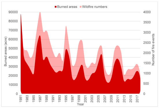
Figure 1.
Numbers of documented wildfires and burned areas due to wildfires in Arkansas from 1981 to 2018.
Arkansas is situated in the south-central part of the United States. It is mainly covered by forests and lakes and has major mountain valleys (Figure 2). The forest landcover occupies more than half of the entire state. Oak covers about 42%, and shortleaf pine occupies 29% of the forest type. About 58% of the timberland is owned by private landowners, such as farmers and ranchers [35]. Nearly 13% of the state’s forested acreage is considered for national forest status, and forest resource companies lease or own about 23% of the state’s timberland [36]. The state’s forest resource provided job opportunities to about 64,789 people in 2011, amounting to USD 3.6 billion of labor income. Additionally, 75% of the energy needed for the forest industries is generated from wood waste [37]. This highlights the value and importance of the forest resource in Arkansas.
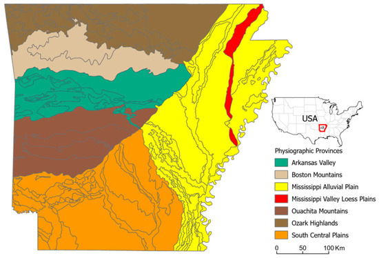
Figure 2.
Physiographic provinces of Arkansas.
In terms of population, the three main population centers are Northwest Arkansas, the Little Rock metropolitan area, and Northeastern Arkansas. Northwest Arkansas, consisting of Fayetteville, Springdale, Bentonville, and Rogers, has more than 525,000 people living in the region, making it the second most populated area in Arkansas [38]. The Little Rock metropolitan area is located at the center of the state, including Jacksonville, Little Rock, Benton, Cabot, Conway, and Maumelle, and approximately 739,000 people live in this area. Northeastern Arkansas, including Jonesboro, is the third main population hub in the state with a population over 100,000 [39].
2.2. Data Acquisition and Processing
The study approach consisted of three major steps: (1) data acquisition and processing for training and prediction, (2) exploring the relationship between fire and selected variables, and (3) geospatial modeling to produce a fire susceptibility map for Arkansas. Four different types of remotely sensed data were acquired for this study, including vegetation, climate, topography, and human intervention factors. The fire incident data were obtained from the Monitoring Trends in Burn Severity (MTBS). MTBS has been collecting fire incident data from 1984 to present, and it is monitored by U.S. Geological Survey’s Earth Resources Observation and Science (EROS) Center and the U.S. Department of Agriculture’s Forest Service Geospatial Technology and Applications Center (GTAC). Using this dataset, fire density was calculated for Oklahoma using the kernel density. The spatial distribution of fire incidents was highly clustered, and thus, the density was estimated by the k-nearest neighbor. The density of each cell was estimated by adding all the values of surfaces where they overlay the cell center. The size of each cell was calculated using the shorter width or height of the extent in the defined coordinate system, divided by 250, to maintain the necessary details for our analysis. Dividing by a smaller number resulted in mixing multiple features and led to the loss of some important information, while dividing by a larger number resulted in a smaller cell size and a larger raster file that required extensive computation.
Vegetation distribution and composition are affected by topographic factors, which themselves are indirectly related to the flammability of forest and climatic influences. Shuttle Radar Topography Mission (SRTM) digital elevation model (DEM) of 1 arc-second spatial resolution was used to derive the elevations for the training and predicting processes. Later, the slope of the study area was extracted from the elevation data.
The landcover map of 2016 was used to identify the burnable vegetation in the study area. Vegetation data of a 30m spatial resolution were obtained from the National Land Cover Database (NLCD). NLCD data divided the landcover into 16 classes, but for the sake of this analysis, the data were reclassified into 7 classes only by combining the similar classes together to reduce multicollinearity among the variables. Then, the vegetation class was subdivided into herb, shrub, tree, and wildland urban interface based on the spatial extent of these subclasses in the dataset obtained from the Landfire program. These subdivisions were necessary to better understand the contribution of various vegetation types to wildfires.
Climatic conditions are also very important for modeling fire susceptibility. Several conditions, such as precipitation, temperature, lighting, and soil moisture, have considerable contributions to fire ignition and propagation, so they were considered in this analysis. Daymet climate data from 1990 to 2015 were used to calculate the average dry season precipitation and annual average temperature [40]. The average annual soil moisture from 1990 to 2015 was estimated from the TerraClimate dataset of a 4km spatial resolution. A thorough examination of the explanatory regression outputs, such as the p-value and R-squared, revealed that annual measures were more suitable than seasonal measures and improved the model performance in some cases; however, the opposite was true in some other cases. Precipitation, directly and indirectly, influences the fire density, and in this study, the influence of precipitation was more noticeable in the dry season (June–October). For temperature and soil moisture, the model showed higher sensitivity to annual averages than seasonal variations.
In addition, the climate water deficit (DEF), potential evapotranspiration (PET), and Palmer drought severity index (PDSI) were used in this study to better understand the wildfire drivers. DEF is the difference between PET and the actual evapotranspiration [41] and helps to estimate the drought stress on soils and plants. PET is the amount of water evaporated by transpiration and evaporation from an area, given a uniform vegetation cover and being well supplied with water. PDSI is designed to calculate the agricultural drought by adding precipitation to the top two layers of the soil and using a temperature-driven evapotranspiration algorithm to remove the moisture. All these metrics are commonly used in fire research [42,43], and thus they were taken into account in this study. Geospatial data of 4 km resolution for these variables were collected for the 1990–2015 period from the TerraClimate dataset for calculating the annual averages.
Human intervention is another important determinant in all wildfire studies. For example, accessibility to protected areas can be represented by road density because roads serve as pathways to the vegetated range and people can intentionally or unintentionally start a fire. Recent investigations have also shown that electricity lines can act as a source of fire ignitions [44]. To determine the effects of road and electricity line networks in the study area, their data were extracted from the Topologically Integrated Geographic Encoding and Referencing (TIGER) database, and then Euclidean distances to the electricity lines and kernel density of the road lines were calculated.
Gridding the study area was found to be an effective way to incorporate all the variables for the model in one attribute. This not only facilitated the desired analysis, but also allowed extracting the required information from different GIS layers to a standard form. Therefore, a fishnet gridding was applied to produce a 10 × 10 km grid for training and predicting purposes, and then a spatial joining was applied to join the required data from different layers to one attribute table. In regression analysis, the data need to be normally distributed, so various transformations, such as log transformation and square root transformation, were applied to standardize the variables.
2.3. OLS and GWR Analyses
The quality and robustness of the predicted model depend mainly on the training data, making the variable selection for training the model critical. To identify significant variables, explanatory regression was applied, and its outputs were used to narrow down the factors that best explained the dependent variable. Variables identified from the explanatory regression were then applied to OLS, which is a linear least-squares method that minimizes the sum of the squares of the differences between the dependent and the independent variables in the given dataset. The least-squares estimator obtains a value that minimizes the sum of squared residuals of the model as the following:
where X is the matrix regressor variable X, T is the matrix transpose, and y is vector of the value of the response variable.
Assumptions such as normality, homogeneity, and independence of residual are taken into account as they are essential for accurate modeling and any violation of these assumptions may lead to inefficient and biased results [45]. OLS produces statistical outputs that can be used to evaluate the model performance. Coefficients represent the type and strength of the relationship between the individual explanatory and dependent variable; they can be either positively or negatively correlated. Analysis of variance (ANOVA) measures whether the model is statistically significant or not by calculating the p-value. The T-test (p-value) developed by Gösset can be used to identify the statistically significant parameters [46].
where is the sample mean from X1, X2, ……, Xn out of a size n, is the population mean, is the standard deviation of the population, S is the standard error of the mean, and Z is the standardized statistic.
In this paper, the sample mean followed the tendency of normal distribution. The consistency in the relationship between the explanatory and the dependent variables over geographic and data spaces was measured by Koenker (BP) statistic. If BP results are statistically significant, this indicates robust probabilities. Multicollinearity, the inter-correlation among model variables, is an important factor to consider when developing a model as it reveals redundancy in model variables that must be removed. Higher multicollinearity leads to higher variance and covariance, eventually leading to unreliable statistical results. The variance inflation factor (VIF) was employed to measure the severity of multicollinearity in the linear regression model. A higher VIF value than 10 indicates severe multicollinearity due to strong associations among the variables in the model. In this study, a VIF threshold <7.5 for all variables was used, and the R-squared and Akaike information criterion (AICc) were used to evaluate the overall model performance. The VIF value can be calculated as the following:
where represents the coefficient of determination between the ith variable Xi and the other variables.
Through the smoothing of local regression, GWR was developed and was later improved with the advancement of statistical measures [47,48,49]. OLS does not consider local variations and geographical data that may vary over space, making it difficult to fit everything into one global equation and may not even represent the true situation. Generally, spatial data are non-stationary, their structure affects the correlation between variables, and the association between variables may vary in space [50]. GWR incorporated spatial heterogeneity as it applies multiple calibrated local regression at each sample point to capture the spatial variation [51]. The GWR general framework can be expressed as:
where I = 1, 2, 3, …, n, (ui,vi) is point of coordinates at point i, Yi is the value of random variable, εi is the random error term, and Xi is the value of a fixed variable that is known and does not contain errors.
The three smoothing functions available in GWR include predefined bandwidth, corrected AICc, and cross validation. GWR provides important diagnostic statistics, such as the standardized residual and the difference between the observed and the calculated values by the model, to understand the local information and evaluate the model performance. The local variations of the adjusted R-squared were used to test how the model explained the dependent variable, and the leverage values were used to measure the influence of the explanatory variables on the model calibration.
2.4. RF Classification
RF is an ensemble ML algorithm developed by Breiman based on decision trees. The number of decision trees generated (nbtree) and the number of selected variables for each split (nbvar) are the two hyperparameters in RF. The RF algorithm bootstrapping is applied to generate nbtree subsets of training dataset from the full dataset with random sampling, with replacement. Bootstrapping improves model stability by averaging all the model outputs. For each of these subsets, RF grows a decision tree by (1) selecting randomly nbvar variables for each split and (2) computing the Gini index and best variables with the best threshold value for the nbvar and output variables for minimizing error in prediction. After successfully training the decision tree, a prediction (ypred) is made from the average of all the decision trees (yi). This produces a robust mean value for prediction by reducing the variance as follows:
Training the RF model for prediction was accomplished by establishing a relationship between the explanatory variables and the variable to predict via building a “forest”. In the training process of building the “forest”, we excluded 20% of the data for validation. The trained model successfully predicted that excluded data and compared them to the observed values to assess the accuracy. RF provides the option to predict a variable as categorical or continuous, as it can predict features beyond the training area; but it must have all the associated explanatory variables of the prediction area that were used in the training.
Following the training, numerous diagnostics, such as the forest characteristics, the out-of-bag (OOB) error, and the summary of variable importance, were employed to assess the model performance. The OOB error can help to evaluate the model performance when 100% of the dataset is used in the training, as it is calculated by the unseen subset of data that is not used in building the “forest”. The variable importance was estimated via the Gini coefficient by calculating the number of times a variable caused split and the impact of that split divided by the number of “trees”. In an unstable RF model, the importance of a variable changes across the validation. By increasing the number of trees, the instability in the model can be decreased. The number of trees, minimum leaf size, maximum tree depth can help to achieve model stability. Increasing the number of trees can make more accurate predictions, but the model takes a longer time to run. In this study, we used 300 “trees” to test the model and excluded 20% of the data for validation. Additionally, we used 5 as the minimum leaf size. Minimum leaf size refers to the number of observations required to keep a terminal node on a tree without further splits, and maximum tree depth refers to the maximum number of splits that will be made. Increasing the number of maximum tree depth can raise the probability of overfitting. The data availability per tree (%) is basically the percentage of input training data used per decision tree. In this study, approximately two-thirds of the randomly sampled data were used in a decision tree. Finally, outputs, such as the R-squared, p-value, and standard error, were used to evaluate the model performance.
3. Results and Discussions
3.1. OLS and GWR Outputs
Considering the explanatory regression results, the following predictors were selected for the analysis: slope, soil moisture, dry season precipitation (June–October), average maximum temperature (Tmax), PET, DEF, PDSI, portion of cultivated area, portion of tree area, portion of herb area, portion of shrub area, portion of barren area, portion of wildland urban interface, road lines density, and distance to electricity lines (Figure 3a–j). The dependent variable was defined as the fire density for both training and prediction. For training the model, the fire density of Oklahoma was selected. The produced fire density map (Figure 4) shows higher fire density in both the northeastern and the southern parts of the state.
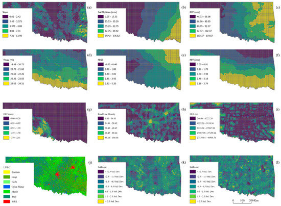
Figure 3.
Selected explanatory variables (grid cell = 10 × 10 km): (a) slope, (b) soil moisture, (c) dry season precipitation (PCP), (d) average maximum temperature (Tmax), (e) Palmer drought severity index (PDSI), (f) potential evapotranspiration (PET), (g) climate water deficit (DEF), (h) road line density, (i) Euclidean distance to electricity lines (DEL), (j) land use/cover, (k) standard deviation (std) of residual from OLS, and (l) standard deviation (std) of residual from GWR.
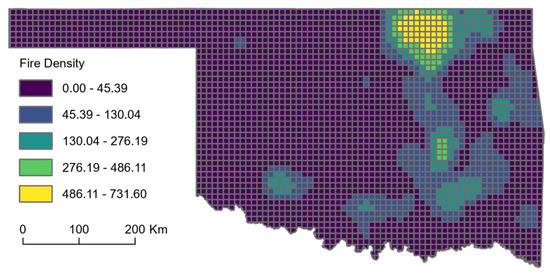
Figure 4.
Fire density map of Oklahoma (grid cell = 10 × 10 km).
After running the OLS, the model showed the expected relation with fire density. The topographic parameter of slope was positively correlated with fire density, suggesting that fire tends to spread at a higher slope than at a lower slope. Vegetation was also positively correlated with fire density. All subclasses of vegetation, including trees, shrubs, and herbs, were positively correlated with fire density, with trees having the strongest influence. Wildland urban interface (WUI) and barren area also showed a positive correlation with fire density. Cultivated land showed a negative correlation with fire density (Table 1) most likely because cultivated areas are frequently monitored and are in private ownership, making the chance of ignition extremely low. The relations between fire density and the selected 15 variables are shown in Figure 5.

Table 1.
Ordinary least squares results. Soil moisture (SM), Euclidean distance to electricity lines (DEL), dry season precipitation (PCP), cultivated area (CA), average maximum temperature (Tmax), potential evapotranspiration (PET), climate water deficit (DEF), road line density (RLD), portion of herb (POH), portion of tree (POT), PDSI (Palmer drought severity index), portion of shrub (POS), wildland urban interface (WUI), portion of barren (POB). Significant p-values < 0.01 are denoted by *; StdError is the standard deviation error; t-Statistic is the ratio between estimated and hypothesized values relative to StdError; probability and robust probability (Pr) are significant when p-values < 0.01 and VIF values < 7.5.
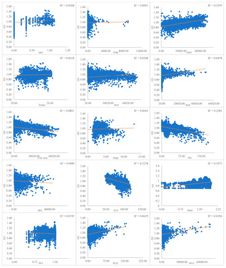
Figure 5.
Scatter plots of fire density versus the selected 15 variables. Soil moisture (SM), Euclidean distance to electricity lines (DEL), dry season precipitation (PCP), cultivated area (Cult. area), average maximum temperature (Tmax), potential evapotranspiration (PET), climate water deficit (DEF), road line density (RLD), portion of herb (POH), portion of tree (POT), PDSI (Palmer drought severity index), portion of shrub (POS), wildland urban interface (WUI), portion of barren (POB).
Dry season precipitation and average maximum temperature tended to have a direct relationship with fire density. As precipitation in the dry season decreased, fire density increased. Additionally, fire density increased as maximum temperature increased. Other positively related factors to fire density included PDSI and DEF. Average soil moisture, however, showed a negative relation with fire density, proving that soil moisture inversely affected fire incidents. Furthermore, PET showed a negative correlation with fire density, along with human-induced factors, such as distance to electric lines, but the road lines density was positively associated with fire density (Table 1).
The p-value for all these explanatory variables is less than 0.1, indicating that these variables are statistically significant. Multicollinearity was tested by VIF. A VIF threshold between 5 and 10 is usually recommended as values out of this range would indicate the existence of collinearity and, thus, redundancy [52,53,54,55]. Among the 15 selected variables, only 4 have VIF values over 5; however, these are the most significantly important factors in modeling fire susceptibility, so a threshold less than 7.5 was applied in this study. Robust probability value is also less than 0.1 (Table 1), adding more confidence to the regression results. The performance of the model is evaluated by the adjusted R-squared value, calculated to be 0.51, meaning that the model can explain nearly half of the observed variation by these explanatory variables (Table 2).
Table 2.
Performance results of OLS and GWR.
OLS was able to explain about 50% of the variance of the dependent variable with the explanatory variables; however, GWR provided better results as the adjusted R-squared value increased from 0.51 to 0.87 (Table 2). This demonstrates that the variables are spatially related, and GWR is superior to OLS in this case for fire density modeling. In this study, the golden search approach was applied to determine the suitable neighbor size. This approach tries to find a suitable number of neighbors based on the lowest AICc value. The findings determined the suitable number of neighbors as 31 with the AICs value of 5171, and GWR provided better results again compared to OLS, adding confidence to the use of these variables in a non-parametric method to predict fire density at a fully different location (Table 2).
3.2. RF Outputs
Fire distribution showed an irregular pattern in the training dataset, and OLS and GWR results indicated that fire density was influenced by both natural and human-related factors. The adjusted R-squared value inferred a nonlinear relationship (Table 2), suggesting that a non-parametric method would be more suitable for this study [18]. This explains why RF outperformed linear regression. A total of 300 “trees” were selected to test the model, and 20% of the data were excluded for validation. The adjusted R-squared value for training the model over Oklahoma was 0.99 with a standard error of 0.002 and a p-value of 0.00, indicating the result is statistically significant. For validation, the adjusted R-squared value was 0.92 with a standard error of 0.01 and a p-value less than 0.00. The validation data share more than 95% of the training data range, indicating that the model is well validated. Overall, the results show that the model is well fitted for prediction. Therefore, the same 15 explanatory variables for the prediction area were fed to the model to predict wildfire densities in Arkansas (Figure 6).
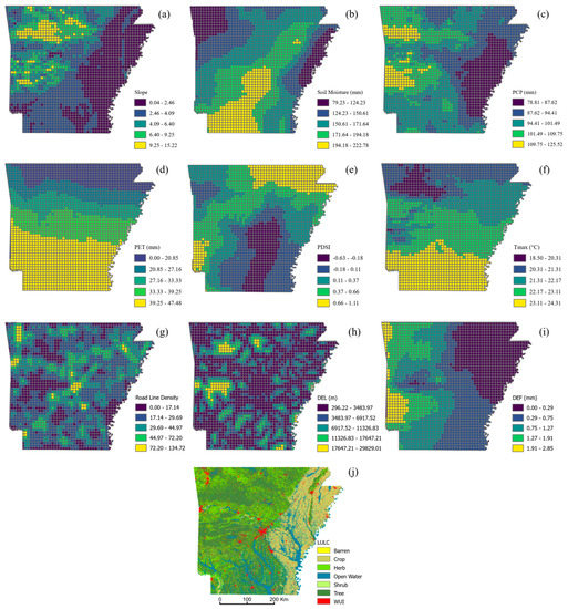
Figure 6.
Identified variables for predicting fire susceptibility in Arkansas (grid cell = 10 × 10 km): (a) slope, (b) average soil moisture, (c) dry season precipitation (PCP), (d) potential evapotranspiration (PET), (e) Palmer drought severity index (PDSI), (f) average maximum temperature (Tmax), (g) road line density, (h) Euclidean distance to electricity lines (DEL), (i) climate water deficit (DEF), and (j) land use/cover.
To predict features at a fully different location, the RF model required all the associated explanatory variables that were used in the training. Thus, a 10 × 10 km grid was created for Arkansas and spatial joining was applied to join the necessary data from different GIS layers to one attribute table. Additionally, a total of 300 “trees” were used in the prediction, but no data were excluded for validation, hence OOB results were utilized to evaluate the model performance. The MSE value for 50% of the “trees” was 924.42, and the percentage of variation explained was 90.14; for 100% of the “trees”, the MSE was 913.81, and the percentage of variation explained was 90.26. The difference in values for both cases was minimal, indicating the number of “trees” had minimal effect on the model outcome.
Of the 15 variables, PET showed the highest importance in RF (Table 3); however, in OLS, it showed a negative strong relationship. The influence of PET on wildfires was explained in details in previous work [56]. Wildland fuels, such as live vegetation, organic soil, and dead fuels, are affected by water deficits; therefore, increasing the water deficit may make fuels drier and more susceptible to ignition and burning [57]. It has been found that summer evapotranspiration has a significant correlation with the wildfires in southwest and southern California [58]. Soil moisture directly influences the dryness of fuels, and affects the dead fuels that are generally found in the ground, so it acts as a proxy to drought [1]. Under low wet conditions at the surface, burnable fuels are more susceptible to burning [59]. PDSI shows significant importance in explaining wildfires, as previous wildfires in the western states have shown a correlation with PDSI [60]. PDSI with precipitation and temperature have been used previously to explain fire events in the 12 ecoregions of the western U.S. [42]. Human factors, as well, have a major influence on fire density. Many reports have identified faulty electricity lines acted as a source of ignition.
Table 3.
Variables used in the analysis and their importance and percentage. Soil moisture (SM), Euclidean distance to electricity lines (DEL), dry season precipitation (PCP), cultivated area (CA), average maximum temperature (Tmax), potential evapotranspiration (PET), climate water deficit (DEF), road line density (RLD), portion of herb (POH), portion of tree (POT), portion of shrub (POS), wildland urban interface (WUI), portion of barren (POB), and Palmer drought severity index (PDSI).
Climatic factors have a significant impact on fire distribution [61]. Average maximum temperature and dry season precipitation have a demonstrated noticeable importance in the model. In this study, average dry season precipitation showed more importance than average maximum temperature. Temperatures above 20 °C promoted wildfires and showed a positive correlation in the linear regression.
The only topographic factor included in this fire modeling is the slope; initially, elevation and aspect factors were also included, but they were eventually excluded due to multicollinearity. The slope of the area showed a notable effect on the RF results, as well as vegetation covers, such as portions of tree, shrub, and herb, which acted as proxies for fuel. In linear regression, these variables demonstrated a significant correlation with fire density. Cultivated area, barren, and WUI also showed some importance in the RF results.
The final stage of RF modeling revealed the predicted fire density for Arkansas, which we categorized into five divisions using an equal interval approach that divided the full range of fire density values into equal-size subranges. Ultimately, the produced five categories were integrated with the fire inventory of Arkansas to create a fire likelihood map for the entire state (Figure 7), assuming that the predicted areas in the highest fire density category are highly susceptible to wildfire and vice versa. Our results indicate that the Ouachita National Forest and the Ozark Forest are highly susceptible to wildfire, while the eastern side of the state is less susceptible to wildfire, and the southern part of the state is moderately susceptible to wildfire. The Ouachita National Forest is close to Little Rock, which is densely populated in central Arkansas, putting this area at high risk. Northwest Arkansas, which is also highly populated, is close to the Ozark Forest, a high-risk zone for wildfires. It is noteworthy that most of the historic fire events coincide with the predicted high susceptibility, which adds more confidence to the established model. Figure 7 shows a strong correlation between the predicted high and high–medium susceptible areas and the documented fires, while it shows weak correlation in the southern part of the state. However, most of the historic fire events in the southern part are just prescribed burns performed to maintain the forest and agricultural production, but they are still documented as wildfires in the archives. The southern part of Arkansas is known as the West Gulf Coastal Plain. It has a gentle slope with rich soil properties and includes extensive areas of loblolly shortleaf pine forests and agricultural fields. Forest harvesting related to hardwood products is predominant in this plain.
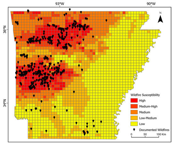
Figure 7.
Documented fire events plotted on top of the modeled fire likelihood for Arkansas (grid cell = 10 × 10 km).
4. Conclusions
Remotely sensed data of moderate spatial resolution (30 m) are capable of elucidating the relationship between the historic fire events and the identified explanatory variables with an acceptable statistical significance. Remote-sensing-based RF is precise and reliable in predicting fire susceptibility beyond the training area at the state level. With higher confidence and accuracy, RF overcomes the limitations of conventional statistical methods in predicting fire vulnerability. This study demonstrates that RF can capture both human influences and contemporary climate changes in fire susceptibility modeling. Among the 15 investigated variables, potential evapotranspiration, soil moisture, Palmer drought severity index, and dry season precipitation were found to be the most significant factors contributing to fire density in Arkansas. The training and validation processes provided significant statistical outputs, indicating high precision in the RF prediction of fire vulnerability. RF outperformed OLS and GWR with an adjusted R-squared value exceeding 0.9. The adjusted R-squared values for OLS and GWR analyses are 0.51 and 0.89, respectively.
The cross checking of the predicted fire susceptibility categories with the documented fire events revealed strong correlations, which highlights the prediction capability of RF that incorporates both physical and human factors. Our modeling results also indicate a strong relationship between fire density and the explanatory variables used in the analysis. Although the relationship between fire density and the contributing factors may vary by location, the model still can be used to identify the main sources of fire. Fire prevention and planning can benefit from these results to better prepare for future fire events and minimize loss by taking necessary precaution measures in a given area according to its local fire drivers.
Author Contributions
Conceptualization, A.A.S. and M.H.A.; methodology, A.A.S. and M.H.A.; software, A.A.S. and M.H.A.; validation, A.A.S. and M.H.A.; formal analysis, A.A.S.; investigation, A.A.S. and M.H.A.; resources, A.A.S. and M.H.A.; data curation, A.A.S.; writing—original draft preparation, A.A.S.; writing—review and editing, M.H.A.; visualization, A.A.S. and M.H.A.; supervision, M.H.A.; project administration, M.H.A.; funding acquisition, M.H.A. All authors have read and agreed to the published version of the manuscript.
Funding
This research was funded by the United States Geological Survey (USGS) and AmericaView, grant number GR013384UAF, awarded to Mohamed H. Aly. The APC was fully waived for this invited paper.
Acknowledgments
Thanks are due to USGS, the National Aeronautics and Space Administration (NASA), the Climatology Lab, and the United States Census Bureau for providing all necessary data for conducting this research. Thanks also to Russell Congalton, the Guest Editor, and three anonymous reviewers for their thorough reviews, constructive comments, and valuable suggestions.
Conflicts of Interest
The authors declare no conflict of interest.
References
- Chuvieco, E.; Aguado, I.; Dimitrakopoulos, A.P. Conversion of fuel moisture content values to ignition potential for integrated fire danger assessment. Can. J. For. Res. 2004, 34, 2284–2293. [Google Scholar] [CrossRef]
- Dickson, B.G.; Prather, J.W.; Xu, Y.; Hampton, H.M.; Aumack, E.N.; Sisk, T.D. Mapping the probability of large fire occurrence in northern Arizona, USA. Landsc. Ecol. 2006, 21, 747–761. [Google Scholar] [CrossRef]
- Dlamini, W.M. A Bayesian belief network analysis of factors influencing wildfire occurrence in Swaziland. Environ. Model. Softw. 2010, 25, 199–208. [Google Scholar] [CrossRef]
- Eugenio, F.C.; dos Santos, A.R.; Fiedler, N.C.; Ribeiro, G.A.; da Silva, A.G.; dos Santos, Á.B.; Paneto, G.G.; Schettino, V.R. Applying GIS to develop a model for forest fire risk: A case study in Espírito Santo, Brazil. J. Environ. Manag. 2016, 173, 65–71. [Google Scholar] [CrossRef]
- Hong, H.; Jaafari, A.; Zenner, E.K. Predicting spatial patterns of wildfire susceptibility in the Huichang County, China: An integrated model to analysis of landscape indicators. Ecol. Indic. 2019, 101, 878–891. [Google Scholar] [CrossRef]
- Pourghasemi, H.R.; Beheshtirad, M.; Pradhan, B. A comparative assessment of prediction capabilities of modified analytical hierarchy process (M-AHP) and Mamdani fuzzy logic models using Netcad-GIS for forest fire susceptibility mapping. Geomat. Nat. Hazards Risk 2016, 7, 861–885. [Google Scholar] [CrossRef]
- Chang, Z.; Du, Z.; Zhang, F.; Huang, F.; Chen, J.; Li, W.; Guo, Z. Landslide Susceptibility Prediction Based on Remote Sensing Images and GIS: Comparisons of Supervised and Unsupervised Machine Learning Models. Remote Sens. 2020, 12, 502. [Google Scholar] [CrossRef]
- Wang, Z.; Lai, C.; Chen, X.; Yang, B.; Zhao, S.; Bai, X. Flood hazard risk assessment model based on random forest. J. Hydrol. 2015, 527, 1130–1141. [Google Scholar] [CrossRef]
- Rouet-Leduc, B.; Hulbert, C.; Lubbers, N.; Barros, K.; Humphreys, C.J.; Johnson, P.A. Machine Learning Predicts Laboratory Earthquakes. Geophys. Res. Lett. 2017, 44, 9276–9282. [Google Scholar] [CrossRef]
- Taalab, K.; Cheng, T.; Zhang, Y. Mapping landslide susceptibility and types using Random Forest. Big Earth Data 2018, 2, 159–178. [Google Scholar] [CrossRef]
- Park, H.; Kim, K.; Lee, D.K. Prediction of Severe Drought Area Based on Random Forest: Using Satellite Image and Topography Data. Water 2019, 11, 705. [Google Scholar] [CrossRef]
- Jaafari, A.; Pourghasemi, H.R. Factors influencing regional-scale wildfire probability in Iran: An application of random forest and support vector machine. In Spatial Modeling in GIS and R for Earth and Environmental Sciences; Elsevier: Amsterdam, The Netherlands, 2019; pp. 607–619. [Google Scholar]
- Breiman, L. Random forests. Mach. Learn. 2001, 45, 5–32. [Google Scholar] [CrossRef]
- Gholamnia, K.; Gudiyangada Nachappa, T.; Ghorbanzadeh, O.; Blaschke, T. Comparisons of Diverse Machine Learning Approaches for Wildfire Susceptibility Mapping. Symmetry 2020, 12, 604. [Google Scholar] [CrossRef]
- McKenzie, D.; Peterson, D.L.; Agee, J.K. Fire Frequency in the Interior Columbia River Basin: Building Regional Models from Fire History Data. Ecol. Appl. 2000, 10, 1497–1516. [Google Scholar] [CrossRef]
- Amatulli, G.; Rodrigues, M.J.; Trombetti, M.; Lovreglio, R. Assessing Long-Term Fire Risk at Local Scale by Means of Decision Tree Technique. J. Geophys. Res Biogeosci. 2006, 111. [Google Scholar] [CrossRef]
- Lozano, F.J.; Suárez-Seoane, S.; Kelly, M.; Luis, E. A Multi-Scale Approach for Modeling Fire Occurrence Probability Using Satellite Data and Classification Trees: A Case Study in a Mountainous Mediterranean Region. Remote. Sens. Environ. 2008, 112, 708–719. [Google Scholar] [CrossRef]
- Oliveira, S.; Oehler, F.; San-Miguel-Ayanz, J.; Camia, A.; Pereira, J.M.C. Modeling spatial patterns of fire occurrence in Mediterranean Europe using Multiple Regression and Random Forest. For. Ecol. Manag. 2012, 275, 117–129. [Google Scholar] [CrossRef]
- Rodrigues, M.; de la Riva, J. An insight into machine-learning algorithms to model human-caused wildfire occurrence. Environ. Model. Softw. 2014, 57, 192–201. [Google Scholar] [CrossRef]
- Song, C.; Kwan, M.-P.; Song, W.; Zhu, J. A Comparison between Spatial Econometric Models and Random Forest for Modeling Fire Occurrence. Sustainability 2017, 9, 819. [Google Scholar] [CrossRef]
- Ouedraogo, I.; Defourny, P.; Vanclooster, M. Application of random forest regression and comparison of its performance to multiple linear regression in modeling groundwater nitrate concentration at the African continent scale. Appl. Hydrogeol. 2018, 27, 1081–1098. [Google Scholar] [CrossRef]
- Chowdhury, E.H.; Hassan, Q.K. Use of Remote Sensing-Derived Variables in Developing a Forest Fire Danger Forecasting System. Nat. Hazards 2013, 67, 321–334. [Google Scholar] [CrossRef]
- Aldersley, A.; Murray, S.J.; Cornell, S. Global and regional analysis of climate and human drivers of wildfire. Sci. Total Environ. 2011, 409, 3472–3481. [Google Scholar] [CrossRef]
- Parisien, M.-A.; Snetsinger, S.; Greenberg, J.; Nelson, C.R.; Schoennagel, T.; Dobrowski, S.; Moritz, M.A. Spatial variability in wildfire probability across the western United States. Int. J. Wildland Fire 2012, 21, 313–327. [Google Scholar] [CrossRef]
- Rodrigues, M.; Jiménez-Ruano, A.; Peña-Angulo, D.; de la Riva, J. A comprehensive spatial-temporal analysis of driving factors of human-caused wildfires in Spain using Geographically Weighted Logistic Regression. J. Environ. Manag. 2018, 225, 177–192. [Google Scholar] [CrossRef]
- Syphard, A.D.; Radeloff, V.C.; Keuler, N.S.; Taylor, R.S.; Hawbaker, T.; Stewart, S.I.; Clayton, M.K. Predicting spatial patterns of fire on a southern California landscape. Int. J. Wildland Fire 2008, 17, 602–613. [Google Scholar] [CrossRef]
- Yang, J.; Weisberg, P.J.; Dilts, T.E.; Loudermilk, E.L.; Scheller, R.M.; Stanton, A.; Skinner, C. Predicting wildfire occurrence distribution with spatial point process models and its uncertainty assessment: A case study in the Lake Tahoe Basin, USA. Int. J. Wildland Fire 2015, 24, 380–390. [Google Scholar] [CrossRef]
- Carlson, J.D.; Burgan, R.E.; Engle, D.M.; Greenfield, J.R. The Oklahoma Fire Danger Model: An operational tool for mesoscale fire danger rating in Oklahoma. Int. J. Wildland Fire 2002, 11, 183–191. [Google Scholar] [CrossRef]
- Reid, A.M.; Fuhlendorf, S.D.; Weir, J.R. Weather Variables Affecting Oklahoma Wildfires. Rangel. Ecol. Manag. 2010, 63, 599–603. [Google Scholar] [CrossRef]
- Weir, J.R.; Reid, A.M.; Fuhlendorf, S.D. Wildfires in Oklahoma; Oklahoma State University: Stillwater, OK, USA, 2012. [Google Scholar]
- Gorte, R.; Economics, H. The Rising Cost of Wildfire Protection. 2013. Available online: https://www.baileyhealthyforests.org/wp-content/uploads/2013/12/fire-costs-background-report.pdf (accessed on 27 January 2022).
- Balch, J.K.; Schoennagel, T.; Williams, A.P.; Abatzoglou, J.T.; Cattau, M.E.; Mietkiewicz, N.P.; St Denis, L.A. Switching on the Big Burn of 2017. Fire 2018, 1, 17. [Google Scholar] [CrossRef]
- Arpaci, A.; Malowerschnig, B.; Sass, O.; Vacik, H. Using multi variate data mining techniques for estimating fire susceptibility of Tyrolean forests. Appl. Geogr. 2014, 53, 258–270. [Google Scholar] [CrossRef]
- Nowak, D.J.; Greenfield, E.J. US Urban Forest Statistics, Values, and Projections. J. For. 2018, 116, 164–177. [Google Scholar] [CrossRef]
- Hodgdon, B.; Tyrrell, M. Literature review: An annotated bibliography on family forest owners. In GISF Research Paper, 2; Yale University: New Haven, CT, USA, 2003. [Google Scholar]
- Clutter, M.; Mendell, B.; Newman, D.; Wear, D.; Greis, J. Strategic Factors Driving Timberland Ownership Changes in the US South; United States Department of Agriculture: Washington, DC, USA, 2003. [Google Scholar]
- Pelkki, M.H. An Economic Assessment of Arkansas’ Forest Industries: Challenges and Opportunities for the 21st Century; Arkansas Agricultural Experiment Station: Fayetteville, AR, USA, 2005. [Google Scholar]
- He, W.; Goodkind, D.; Kowal, P. International Population Reports. In An Aging World: 2015; US Census Bureau: Suitland, MD, USA, 2016. [Google Scholar]
- Rowden, K.W.; Aly, M.H. GIS-based regression modeling of the extreme weather patterns in Arkansas, USA. Geoenviron. Disasters 2018, 5, 6. [Google Scholar] [CrossRef][Green Version]
- Thornton, P.E.; Thornton, M.M.; Mayer, B.W.; Wilhelmi, N.; Wei, Y.; Devarakonda, R.; Cook, R.B. Daymet: Annual Climate Summaries on a 1-km Grid for North America, 2nd ed.; ORNL DAAC: Oak Ridge, TN, USA, 2018.
- Stephenson, N. Actual evapotranspiration and deficit: Biologically meaningful correlates of vegetation distribution across spatial scales. J. Biogeogr. 1998, 25, 855–870. [Google Scholar] [CrossRef]
- Littell, J.S.; McKenzie, D.; Peterson, D.L.; Westerling, A.L. Climate and wildfire area burned in western US ecoprovinces, 1916–2003. Ecol. Appl. 2009, 19, 1003–1021. [Google Scholar] [CrossRef]
- Miller, J.D.; Skinner, C.N.; Safford, H.D.; Knapp, E.E.; Ramirez, C.M. Trends and causes of severity, size, and number of fires in northwestern California, USA. Ecol. Appl. 2012, 22, 184–203. [Google Scholar] [CrossRef]
- Miller, C.; Plucinski, M.; Sullivan, A.; Stephenson, A.; Huston, C.; Charman, K.; Prakash, M.; Dunstall, S. Electrically caused wildfires in Victoria, Australia are over-represented when fire danger is elevated. Landsc. Urban Plan. 2017, 167, 267–274. [Google Scholar] [CrossRef]
- Montgomery, D.C.; Peck, E.A.; Vining, G.G. Introduction to Linear Regression Analysis, 5th ed.; John Wiley & Sons: Chicester, UK, 2013; Available online: http://uark.summon.serialssolutions.com/2.0.0/link/0/eLvHCXMwdV3PS8MwFH7M7TLxoNPhr0nPQkvbrPlxGsxt3YRexPtIm9SDUGGrsD_fl6RxIPMYEhISkpfvJd_7HgBJozj8YxNqKtOSS1HHVVWJWnJeJmg0p0okQiurq50XZLlgr2u66EHhQ2Psj2FHU4y8rTz-pcrdZ2ib7DvGZeSiAWbKAVz0bvAQnaFLFmd9GMw3-Tz3uw09i5SKI1hIEFhwTqlNJ5Qg0GeEik4UypczQ5WWNoWLv4JWlzDQJi7hCnq6GcF58Su3uh_B0EBGp7h8Dc8bQz5XThU2aL8CdDdxOwdv-sNxXpvAK5HcwGS1fH9Zh2a0bfeSsy2JwOkQcSBjuJCGAd-0NlJO3ULApLY3TYKYblqzWKisrDJOpBZMpZLfwfh0Z_f_VTzAMLXJH8yDwyP02923nrgFeOoW8wfsm4i3 (accessed on 27 January 2022).
- Gösset, W.S. The probable error of a mean. Biometrika 1908, 6, 1–25. [Google Scholar]
- Brunsdon, C.; Aitkin, M.; Fotheringham, S.; Charlton, M. A comparison of random coefficient modelling and geographically weighted regression for spatially non-stationary regression problems. Geogr. Environ. Model. 1999, 3, 47–62. [Google Scholar]
- Páez, A.; Uchida, T.; Miyamoto, K. A general framework for estimation and inference of geographically weighted regression models: 1. Location-specific kernel bandwidths and a test for locational heterogeneity. Environ. Plan. A 2002, 34, 733–754. [Google Scholar] [CrossRef]
- Fotheringham, A.S.; Brunsdon, C.; Charlton, M. Geographically Weighted Regression: The Analysis of Spatially Varying Relationships; John Wiley & Sons: Hoboken, NJ, USA, 2003. [Google Scholar]
- Hanham, R.; Spiker, J.S. Urban sprawl detection using satellite imagery and geographically weighted regression. In Geo-Spatial Technologies in Urban Environments; Springer: Berlin/Heidelberg, Germany, 2005; pp. 137–151. [Google Scholar]
- Zhang, L.; Bi, H.; Cheng, P.; Davis, C.J. Modeling spatial variation in tree diameter–height relationships. For. Ecol. Manag. 2004, 189, 317–329. [Google Scholar] [CrossRef]
- Petter, S.; Straub, D.; Rai, A. Specifying Formative Constructs in Information Systems Research. MIS Q. 2007, 31, 623–656. [Google Scholar] [CrossRef]
- Cenfetelli, R.T.; Bassellier, G. Interpretation of formative measurement in information systems research. MIS Q. 2009, 33, 689–707. [Google Scholar] [CrossRef]
- Hair, J.F. Multivariate Data Analysis; Prentice Hall: Hoboken, NJ, USA, 2009. [Google Scholar]
- Kline, R.B. Principles and Practice of Structural Equation Modeling; Guilford Publications: New York, NY, USA, 2015. [Google Scholar]
- Kane, V.R.; Cansler, C.A.; Povak, N.; Kane, J.T.; McGaughey, R.J.; Lutz, J.; Churchill, D.J.; North, M.P. Mixed severity fire effects within the Rim fire: Relative importance of local climate, fire weather, topography, and forest structure. For. Ecol. Manag. 2015, 358, 62–79. [Google Scholar] [CrossRef]
- Dimitrakopoulos, A.P.; Mitsopoulos, I.D.; Gatoulas, K. Assessing ignition probability and moisture of extinction in a Mediterranean grass fuel. Int. J. Wildland Fire 2010, 19, 29–34. [Google Scholar] [CrossRef]
- Abatzoglou, J.T.; Kolden, C.A. Relationships between climate and macroscale area burned in the western United States. Int. J. Wildland Fire 2013, 22, 1003–1020. [Google Scholar] [CrossRef]
- Bartsch, A.; Balzter, H.; George, C. The influence of regional surface soil moisture anomalies on forest fires in Siberia observed from satellites. Environ. Res. Lett. 2009, 4, 045021. [Google Scholar] [CrossRef]
- Collins, B.M.; Omi, P.N.; Chapman, P.L. Regional relationships between climate and wildfire-burned area in the Interior West, USA. Can. J. For. Res. 2006, 36, 699–709. [Google Scholar] [CrossRef]
- Drever, C.R.; Drever, M.C.; Messier, C.; Bergeron, Y.; Flannigan, M. Fire and the relative roles of weather, climate and landscape characteristics in the Great Lakes-St. Lawrence forest of Canada. J. Veg. Sci. 2008, 19, 57–66. [Google Scholar] [CrossRef]


Publisher’s Note: MDPI stays neutral with regard to jurisdictional claims in published maps and institutional affiliations. |
© 2022 by the authors. Licensee MDPI, Basel, Switzerland. This article is an open access article distributed under the terms and conditions of the Creative Commons Attribution (CC BY) license (https://creativecommons.org/licenses/by/4.0/).