Binary Logistic Regression Outperforms Decision Tree Modeling for Event-Based Landslide Prediction: Application to Dynamic Hazard and Threshold Mapping in Central Italy

Abstract

The increasing frequency of disasters caused by landslides, mainly due to climate change leading to more intense extreme events, requires reliable predictive models for risk mitigation. Italy, in particular, is a country at high risk of landslides, but the lack of an updated catalogue of landslide activation dates poses a significant challenge for defining reliable activation thresholds. This study develops a methodology for mapping landslide susceptibility based on events in a pilot area of central Italy, integrating a database of landslides with known activation dates with predisposing and triggering parameters. Two statistical techniques were compared to assess their predictive performance in discriminating landslide from non-landslide conditions during extreme precipitation events. A comparison between binary logistic regression (BLR) and decision trees (QUEST) revealed the clear superiority of the BLR model, which achieved excellent predictive accuracy (AUC = 0.913). The model identified clay-rich lithology, gentle slopes (0–16°) and maximum daily precipitation as the most significant controlling factors. This result led to the generation of three derivative products: a susceptibility map, a hazard map for an extreme precipitation scenario with a 100-year return period, and a spatially distributed map of activation thresholds. This threshold map quantifies the intensity of precipitation required to exceed a critical probability of landslide initiation (p > 0.7) at any point in the territory. The susceptibility map highlights critical areas within the study area, while the hazard map also includes the return period of the event. The threshold map is a direct and operational tool for early warning systems, transforming a statistical model into a guide for real-time risk management. The study area serves as a pilot area that could allow this methodology to be replicated. With the integration of real-time meteorological data, it could function as a real-time warning system. The proposed framework therefore provides a directly actionable tool for civil protection agencies, land-use planning authorities, and emergency managers, enabling location-specific rainfall alert thresholds to be issued rather than a single regional value, with the potential to reduce both false alarms and missed warnings.

1. Introduction

Recent studies estimate a global rise in landslide-related disasters over the past decades, attributed to both increasing exposure (population, infrastructure) and stronger climatic drivers [1]. Italy, a country with a densely populated territory and a high concentration of cultural heritage, is one of the European countries with the highest exposure to landslide risk, with 636,000 landslides recorded by the IFFI (Inventory of Italian Landslides) project [2]. Surveys conducted in 2024 compared to those conducted in 2021 showed a 15% increase in landslide surface area, with 23% of Italian territory subject to landslide risk [3]. Climate change, which causes increasingly intense and sudden extreme precipitation events, triggers landslides, especially debris flows, mud flows, rotational landslides, and translational landslides [4]. The definition of activation thresholds and the estimation of landslide probability represent fundamental research objectives, as they underpin early warning systems and risk mitigation strategies aimed at protecting buildings, infrastructure, and human lives. To date, most landslide susceptibility mapping studies have not incorporated activation dates or event-specific triggering conditions [5]. They typically rely on multi-temporal inventories to identify areas sharing geomorphological or climatic characteristics with past landslides, without distinguishing between landslides of different ages or triggered by different processes [6]. This static, inventory-driven approach conflates heterogeneous landslide populations and cannot capture the conditional probability of failure given a specific precipitation trigger, thereby limiting its utility for operational applications such as event-based early warning. Two more advanced research directions have emerged in response to these limitations. Dynamic landslide hazard modelling integrates susceptibility assessments with precipitation or seismic-hydrological trigger models, yielding hazard maps with an explicit temporal dimension, such as probability maps conditioned on predicted rainfall [7,8]. Event-based susceptibility mapping, by contrast, constructs inventories restricted to landslides triggered by a single extreme event, thereby calibrating models to event-specific triggering conditions and producing outputs that are more directly interpretable in an operational context [9,10]. However, a critical methodological gap persists: existing event-based studies rarely combine event-specific model calibration with a statistically invertible probabilistic framework capable of producing spatially distributed, operationally applicable activation thresholds. Without this inversion step, whereby the calibrated model is solved for the precipitation intensity required to exceed a critical failure probability at each location, susceptibility outputs remain difficult to translate directly into rainfall-based warning criteria for civil protection agencies. A further prerequisite for event-based analysis in the Italian context is the availability of reliable landslide activation dates. No systematic national catalogue of activation dates currently exists in Italy, which precludes the direct construction of event-specific inventories and the derivation of calibrated precipitation thresholds [5]. To address this constraint, researchers have employed remote sensing techniques to retrospectively reconstruct activation dates. Visual interpretation and manual or unsupervised sampling of landslide areas using pre- and post-event imagery represent one approach [11,12]. Alternatively, satellite-derived spectral indices compared across multiple events have yielded promising results [13]. Once an event-specific landslide database is established, the choice of statistical framework becomes critical. Three approaches are most commonly applied to probabilistic susceptibility analyses and threshold definition: binary logistic regression (BLR), decision trees (DT), and random forests (RF). Binary logistic regression provides calibrated parametric probabilities and allows direct significance tests; however, it relies on the logit link function and a linear combination of predictors, which may limit its ability to capture complex nonlinear geomorphological processes [14]. Decision trees, in contrast, provide interpretable rule-based thresholds that can identify critical triggering conditions, making them particularly suitable for early warning and decision-support applications; their drawbacks include a tendency to overfit and instability when applied to small or noisy datasets [15]. Random forests, by aggregating multiple trees, produce more robust probabilistic predictions and reduce model variance, but at the expense of interpretability, as they do not provide explicit threshold values readily applicable in practice [16]. The scientific literature presents mixed evidence on the relative performance of these methods. Several studies emphasize the advantages of BLR over RF and DT for susceptibility mapping when interpretability and statistical inference are paramount. Others report superior performance of RF; for example, Ref. [17] found that RF and XGBoost outperformed logistic regression along the upper Jinsha River, with RF exceeding logistic regression by 20.34% in accuracy and 0.1829 in AUC. Conversely, Ref. [18] reported higher performance for logistic regression than RF in Malaysia. Method selection largely depends on dataset characteristics: BLR tends to outperform tree-based methods in small-sample, class-imbalanced scenarios because its maximum likelihood estimation is more stable and it directly models minority-class probabilities [19,20,21], whereas RF and DT are favoured when nonlinear predictor relationships dominate [22,23]. Nonetheless, numerous studies, including some in the medical field, demonstrate that BLR can outperform machine learning approaches under specific conditions [24]. The present study addresses these gaps through an event-based susceptibility analysis calibrated on multiple extreme precipitation episodes in a pilot region of central Italy, for which an extensive database of landslides with reconstructed activation dates is available. The specific objectives are threefold: (1) to compare BLR and the QUEST decision tree algorithm in terms of predictive performance under class-imbalanced, event-specific conditions; (2) to derive spatially distributed activation thresholds by inverting the calibrated probabilistic model, thereby translating statistical outputs into operationally applicable rainfall triggers; (3) to produce a suite of three complementary products, a susceptibility map, a 100-year return-period hazard map, and a spatially distributed threshold map, providing a transferable methodological framework for data-scarce regions. Seven predictor variables are considered: land use, lithology, slope aspect, slope gradient, maximum daily precipitation, antecedent soil saturation, and cumulative event precipitation [25].

2. Methods

2.1. Study Area

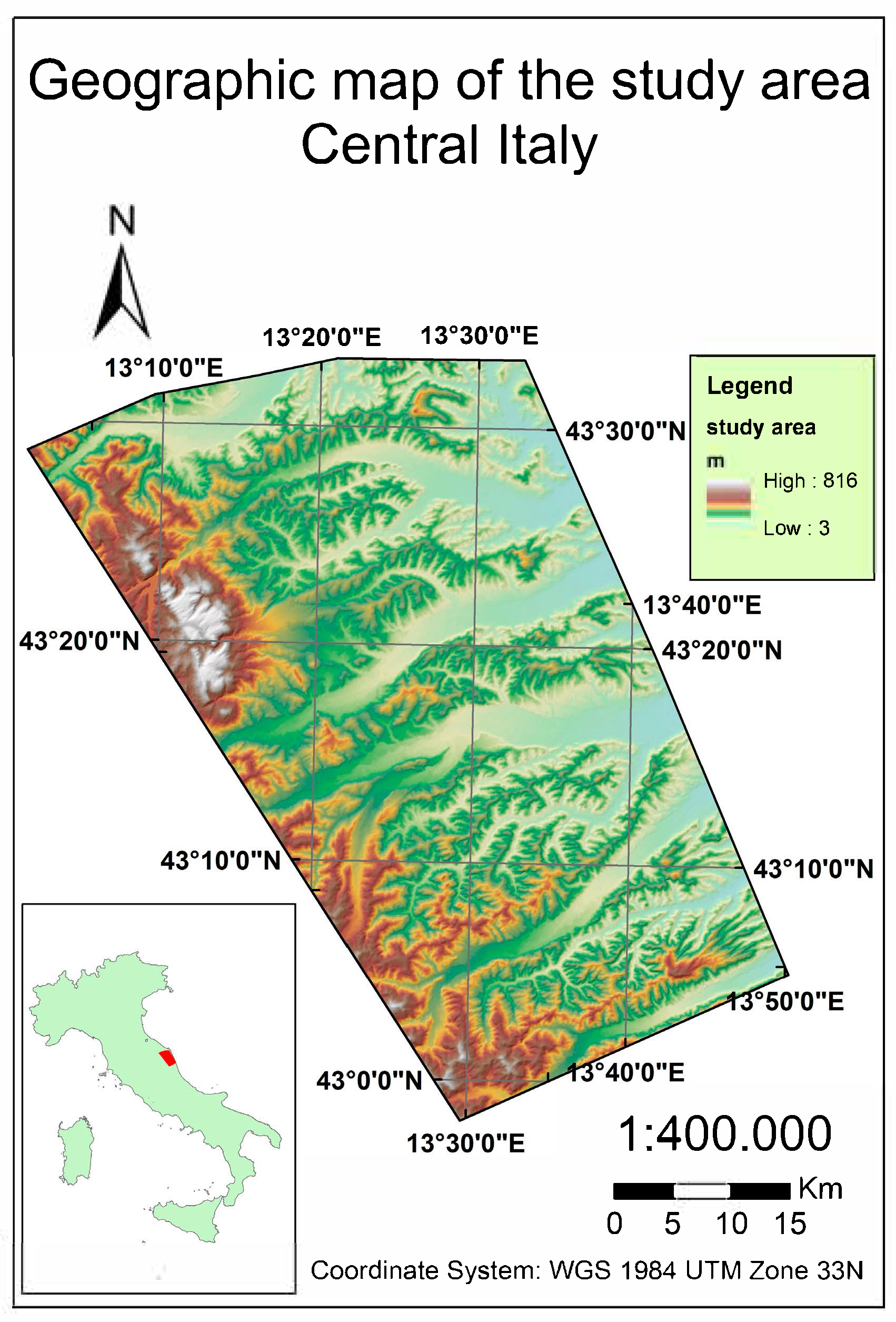
The study was conducted in a pilot area of approximately 2334 km² in central Italy along the Adriatic coast, encompassing both coastal areas and hilly and mountainous areas (Figure 1). This spatial delimitation was adopted to maximise the availability of Landsat imagery, thereby increasing the number of temporal acquisitions suitable for analyzing the extreme event under investigation.

The area is highly heterogeneous in terms of elevation, ranging from sea level to over 800 m. At higher elevations, rockfalls and toppling are more frequent due to the greater exposure of the limestone bedrock. However, the prevailing formations in the area consist mainly of marly limestone, marl, and clay, which are more prone to slope failures, debris flows, and mudflows.

2.2. Logistic Regression

The statistical analysis aimed at defining threshold and probability values was conducted using binary logistic regression and compared with decision tree models. Binary logistic regression demonstrated the best performance and was therefore adopted to model the relationship between the dichotomous outcome variable and a set of predictor variables. This method is particularly suitable because it estimates the probability of an event occurring through the logistic function, which transforms the linear predictor into a value bounded between 0 and 1. The model is expressed as [26]:

$$P\left(Y=1\right)={\displaystyle \frac{1}{1+e^{-({\beta }_0+{\beta }_1{X}_1+{\beta }_2{X}_2+\dots +{\beta }_k{X}_k)}}}$$

(1)

where

$P\left(Y=1\right)$ is the probability of the event.

${\beta }_0$ is the intercept.

${\beta }_1{,\beta }_2$… are the regression coefficients for predictors $X_1,X_2\dots$.

$e$ = base of the natural logarithm (Euler’s number, ≈2.718).

The exponential of each coefficient quantifies the change in the odds of the outcome associated with a one-unit increase in the corresponding predictor. Model significance was assessed using the likelihood ratio test, while the contribution of individual predictors was evaluated through Wald’s chi-square statistics and the associated p-values [27]. The discriminatory power and overall accuracy of the model were evaluated by analyzing the area under the Receiver Operating Characteristic (ROC) curve (AUC), with an AUC of 1.0 indicating perfect discrimination and 0.5 representing random discrimination [27]. The optimal probability cut-off for classification was determined using Youden’s Index (J), which maximizes both sensitivity and specificity. Finally, the model’s goodness-of-fit was further verified through the Hosmer–Lemeshow test.

2.3. Decision Tree Quest

The decision tree was developed using the Quick, Unbiased, Efficient Statistical Tree (QUEST) algorithm, implemented in XLSTAT. QUEST is specifically designed to reduce variable selection bias while ensuring statistically rigorous and computationally efficient splitting procedures. At each node, the algorithm identifies the most informative predictor by means of statistical tests assessing the association between candidate variables and the dependent variable. For categorical predictors, Pearson’s chi-square test of independence is applied, whereas for continuous predictors the F-test of equality of means is employed. The predictor variable $X_j$ that maximizes the test statistic, or equivalently minimizes the corresponding p-value, is selected for the splitting variable. Formally, given a set of predictors $\left\{X_1,X_2,\dots \dots ,X_p\right\}$ and a binary response variable $Yϵ\left\{\mathrm{0,1}\right\}$, the algorithm identifies [28]:

$$X^{*}=arg\underset{\mathit{jϵ}\left\{1,\dots ,p\right\}}{\min }p-value\left(X_j,Y\right)$$

(2)

where the p-value is obtained from the appropriate test depending on the type of $X_j$. Once the splitting variable is selected, QUEST determines the optimal cut-point using quadratic discriminant analysis (QDA) for continuous predictors, or by grouping categories for categorical predictors. This procedure ensures that each partition is based on robust statistical criteria, thereby avoiding the tendency of traditional algorithms such as CART to favor variables with a larger number of categories. The analysis was conducted on a training dataset, while model performance was evaluated on an independent validation dataset to prevent overfitting and to assess generalizability. The Receiver Operating Characteristic (ROC) curve was also generated to evaluate the discriminatory capacity of the model, and the area under the curve (AUC) was computed to quantify classification accuracy, with higher values reflecting greater predictive ability. This methodological framework not only identifies the most relevant explanatory variables but also produces an interpretable set of decision rules, clarifying how different combinations of factors contribute to the probability of landslide occurrence.

2.4. Dataset and Analysis

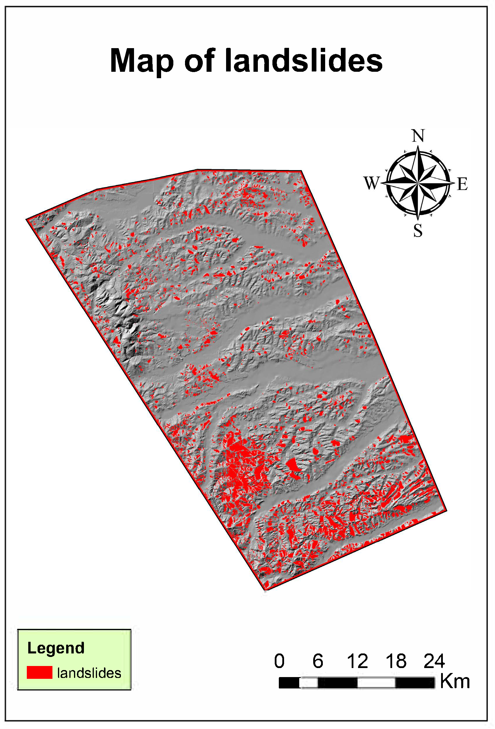
Approximately 13,000 landslides relevant to this study were identified in the study area, including mudflows, debris flows, and translational slides (Figure 2).

From these, around 3000 landslides were randomly selected using ArcGIS 10.8 software. This subset included both landslides triggered during the extreme precipitation events of 2008, 2010, and 2011, as well as events recorded in the national IFFI database (Inventory of Landslide Phenomena in Italy). The extreme precipitation episodes occurred between 5–7 March 2008, 9–10 March 2010, and 1–13 March 2011. During these three events, 250 landslides were triggered, reconstructed through a model based on remote sensing using satellite-derived spectral indices. This approach enabled the integration of ground-based monitoring data with satellite-derived information, thereby extending the available dataset. To address the imbalance between stable areas and landslide-affected areas, a weighting factor was incorporated into the model. A validation dataset of 900 landslides was also prepared, including 78 landslides triggered during the extreme events. On this basis, the data were statistically analyzed according to seven parameters:

• Land use, derived from Corine Land Cover at the first level, classified into 5 categories [29]: agricultural surfaces, artificial surfaces, semi-natural wooded territories, wetlands, and water bodies.
• Slope gradient, classified into 4 classes [6]: 0–16°, 16–25°, 25–35°, and >35°.
• Lithology, classified into 6 categories [6]: clays and marly clays with intercalations of sandstone, sands and conglomerates; deposits; limestones, flinty limestones, subordinately marls and clay marls; marls, clay marls and marly limestones; sandstones, marly clays, subordinately conglomerates; shales and marls encompassing calcareous, marly limestones and arenaceous bodies.
• Slope aspect, classified into 9 categories: flat, north, north-east, east, south-east, south, south-west, west, and north-west.
• Topographic Wetness Index (TWI), classified into 7 classes [30]: 0–2, 2–4, 4–6, 6–8, 8–10, 10–12, and 12–23.
• Antecedent soil saturation, expressed as a percentage for the day preceding the extreme precipitation event.
• Maximum daily precipitation during the event, expressed in mm.
• Cumulative precipitation over the duration of the extreme event, expressed in mm.

All data were georeferenced, rasterized, and processed in ArcGIS 10.8. Each landslide was attributed with the values of the seven parameters corresponding to its spatial location. The resulting dataset was then exported into Microsoft Excel and subsequently analyzed in XLSTAT using binary logistic regression (BLR) and the QUEST decision tree algorithm. Both annual analyses (for each extreme event separately) and a collective analysis (including all years) were performed to identify the most effective statistical approach, which was then used to develop the reference model. Based on this model, a landslide susceptibility map was generated using the mean maximum daily precipitation, also rasterized. A hazard map was subsequently produced by applying the Generalized Extreme Value (GEV) method to the maximum daily precipitation series (1991–2020), in order to simulate extreme-event scenarios. Finally, a precipitation threshold map was created by setting the landslide probability above 0.7 in the probability equation derived from the model.

2.5. Precipitation Data Processing

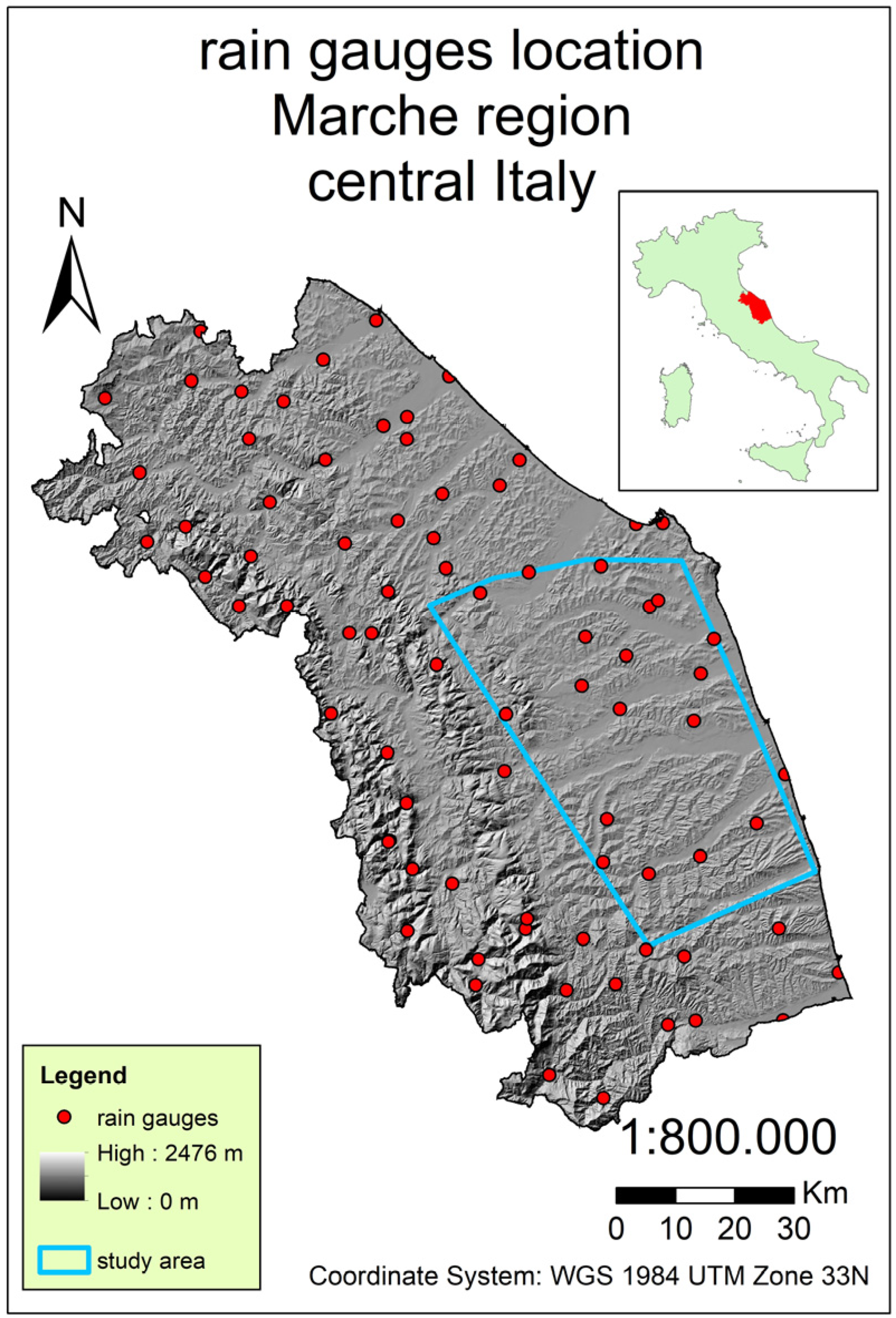
With regard to precipitation, two variables were analyzed during the selected extreme events: cumulative precipitation over the entire event and maximum daily precipitation. For this purpose, data from 80 rain gauge stations were obtained from the regional meteorological network SIRMIP online (Regional Weather-Hydro-Rainfall Information System). Precipitation records were collected starting 15 days prior to each event and were also used to estimate soil saturation conditions. Daily precipitation values were interpolated using the Empirical Bayesian Kriging (EBK) method to generate raster surfaces within the GIS environment, thereby enabling spatially continuous representation of rainfall patterns for subsequent analyses. The interpolation domain was defined to encompass the full spatial extent of the landslide inventory, ensuring that all landslide sample locations fall within the interpolated precipitation surface and that no sample point lies outside the coverage of the gauge network used for EBK spatialization. In addition, maximum daily precipitation data covering the period 1991–2020 were collected from 131 rain gauges distributed over a wider area than the study region, in order to improve the spatialization of boundary conditions. From these records, mean values were computed to provide a robust regional baseline (Figure 3).

Furthermore, these data were employed to compute the 100-year daily return level by applying the Generalized Extreme Value (GEV) distribution within the framework of Extreme Value Theory (EVT). EVT provides a probabilistic basis for modeling the tail behavior of distributions. The Generalized Extreme Value (GEV) distribution describes block maxima (e.g., annual maxima) and, depending on the shape parameter k, dictates the type of the limiting distribution: Gumbel (k = 0), Fréchet (k > 0), or Weibull (k < 0). The model is parameterized by location (μ), scale (σ), and shape (k), and its domain is constrained by the condition 1 + k(x − μ)/σ > 0 for k ≠ 0. Parameter estimation was performed using Maximum Likelihood Estimation (MLE), which yielded the return levels [29],

$$z_p=\mu +{\displaystyle \frac{\sigma }{k}}\left({\left[-\log (1-p)\right]}^{-k}-1\right)$$

(3)

along with their associated confidence intervals. The model’s goodness-of-fit was assessed using diagnostic plots (quantile-quantile, histogram, and return level plots) generated with the in2extRemes package in R 4.2.1 [31]. The diagnostics confirmed a satisfactory alignment between the observed data and the theoretical model [29,32]. As expected, the confidence intervals widen with increasing return periods, reflecting greater uncertainty in extrapolating to more extreme events.

2.6. Saturation Data Processing

Soil saturation during the 15-day period preceding an extreme precipitation event was estimated using soil texture data (i.e., sand, silt, and clay fractions) and bulk density ($p_b)$, sourced from the European Soil Data Centre [33]. The requisite hydraulic parameters were derived by applying the pedotransfer functions established by Cosby et al. (1984) [34]. These functions enable the estimation of soil water retention properties and saturated hydraulic conductivity based on fundamental soil properties. The soil water retention curve was characterized by a log-linear relationship between soil water potential (ψ, cm) and volumetric water content (θ, cm³ cm⁻³) [34]:

$$\theta \left(\psi \right)={\theta }_s{\left({\displaystyle \frac{\psi }{{\psi }_e}}\right)}^{-b}$$

(4)

where θ(ψ) is the volumetric water content at a given matric potential ψ, θ_s is the saturated water content, ψ_e is the air entry potential (cm), and b is the slope parameter of the soil water retention. The saturated water content was estimated as a function of bulk density $p_b$ following [35]:

$${\theta }_s=1-\left({\displaystyle \frac{p_b}{p_p}}\right)$$

(5)

where θ_s is the saturated volumetric water content, $p_b$ is the soil bulk density (g cm⁻³), and $p_p$ is the particle density, assumed equal to 2.65 g cm⁻³. The soil water potential at −33 kPa (field capacity, ${\theta }_{fc}$) and at −1500 kPa (wilting point, ${\theta }_{wp}$) were then derived using the regression equations of [34], which relate texture fractions to retention at given matric potentials [34]:

$${\log }_{10}\left({\psi }_{1/3}\right)=2.17+0.00057 \ast \left(\%{clay}^2\right)-0.00035 \ast \left({\%silt}^2\right)-0.00048 \ast (\%sand)$$

(6)

where ${\psi }_{1/3}$ and ψ₁₅ are the soil water potentials corresponding to field capacity (−33 kPa) and wilting point (−1500 kPa) [34].

$${\log }_{10}\left({\psi }_{15}\right)=4.09+0.00045 \ast \left(\%{clay}^2\right)-0.00038 \ast \left({\%silt}^2\right)-0.00047 \ast \left(\%sand\right)$$

(7)

Combining Equations (3), (5) and (6), the values of ${\theta }_{fc}$ and ${\theta }_{wp}$ were calculated. Saturated hydraulic conductivity ($K_s$) was also estimated as [34]:

$$K_s=1930 \ast {\psi }_e^{2b}$$

(8)

${\psi }_e$ = air entry suction (cm), i.e., the matric potential at the point of air entry into the soil.

b = slope parameter of the soil water retention curve, empirically estimated as [34]:

$$b=3.10+0.157 \ast \left(\%clay\right)-0.003 \ast (\%silt)$$

(9)

The term ${\psi }_e^{2b}$ therefore represents the combined influence of the air entry suction ${\psi }_e$ and the slope of the retention curve (b) on hydraulic conductivity, thereby constraining water fluxes and percolation in the daily water balance (8). Daily volumetric water content (${\theta }_t$) between 15 and 1 day before the event was then updated through a simple soil water balance model [36]:

$${\theta }_t={\theta }_{t-1}+{\displaystyle \frac{P-ET-Q-D}{Z}}$$

(10)

where $P$ is P daily precipitation, ET evapotranspiration, Q surface runoff, D drainage losses, and $Z$ the depth of the considered soil layer. The computed ${\theta }_t$ was constrained between ${\theta }_{wp}$ ≤ ${\theta }_t$ ≤ ${\theta }_s$. Finally, soil saturation was expressed as a percentage through the following equation [34]:

$$S\left(t\right)={\displaystyle \frac{{\theta }_t}{{\theta }_s}}\ast 100$$

(11)

thus allowing the reconstruction of the temporal evolution of soil saturation until 1 day prior to the triggering rainfall [33,34,35,36].

The application of the [34] pedotransfer functions rests on three key assumptions that should be explicitly acknowledged: soil hydraulic properties are determined primarily by texture fractions (sand, silt, and clay percentages), with the influence of organic matter and structural heterogeneity considered negligible; the soil profile is treated as a single homogeneous layer of uniform depth Z, neglecting vertical stratification; the water balance model assumes one-dimensional vertical drainage, without accounting for lateral subsurface flows. These simplifications may introduce uncertainty, particularly in heterogeneous or stratified soils such as those found in clay-rich lithologies with interbedded sands and conglomerates. Furthermore, the antecedent saturation period was fixed at 15 days prior to each triggering event, following the characteristic soil drainage timescales identified by [36] for clay-dominated lithologies. Although this choice is physically motivated, the use of alternative time windows (e.g., 7-day or 30-day antecedent periods) may be more appropriate in different lithological or seasonal contexts. A sensitivity analysis on this parameter is therefore identified as a valuable direction for future research. Direct calibration of the soil saturation estimates against in situ soil moisture measurements was not possible in this study due to the absence of a spatially dense network of field sensors in the study area; this represents a methodological limitation that is explicitly acknowledged. Importantly, however, the influence of antecedent soil saturation on the final model was found to be minimal. The variable was excluded from the refined BLR model due to multicollinearity and an anomalously unstable coefficient (β = −19.06), indicating substantial informational redundancy with the precipitation-related predictors. This result suggests that, in the present dataset and study area, the soil saturation proxy computed from the pedotransfer functions does not provide an independent predictive contribution, and its removal did not compromise model performance (AUC = 0.913). The methodological uncertainties associated with the pedotransfer function assumptions therefore have a limited bearing on the main conclusions of this study.

3. Results

3.1. Statistical Analysis of BLR

The primary drivers of landslides are not static but highly dynamic, varying substantially according to the specific climatic and hydrological conditions preceding each event. An initial comprehensive binary logistic regression (BLR) model was constructed using Firth’s penalized-likelihood method to mitigate potential separation issues. This model incorporated all available predictors: topographic wetness index (TWI), soil saturation, cumulative rainfall, maximum daily precipitation intensity, land cover (CLC), slope gradient, lithology, and aspect. Although the full model showed excellent discriminative ability (AUC = 0.941), diagnostic checks revealed significant multicollinearity, particularly among hydrological variables, as indicated by a correlation coefficient of 0.96 between cumulative and maximum daily precipitation. Moreover, the coefficient for soil saturation was anomalously large and unstable (β = −19.06), a typical symptom of quasi-complete separation, suggesting substantial informational redundancy with precipitation-related variables. The TWI variable also exhibited a counterintuitive negative coefficient, suggesting it failed to provide a meaningful independent contribution within its realistic value range, likely due to collinearity with other topographic factors such as slope gradient. To improve model parsimony, stability, and operational utility for real-time early warning, a refined model was developed by removing the collinear and problematic variables (TWI, soil saturation, and cumulative rainfall). The resulting model, which retains maximum daily precipitation intensity, slope, lithology, aspect, and land cover, maintained very strong predictive performance (AUC = 0.91). A non-significant result of the Hosmer–Lemeshow test (p = 0.540) indicated good calibration between predicted and observed probabilities. Model fit statistics (McFadden’s R² = 0.45; Nagelkerke’s R² = 0.52) confirmed that the selected predictors jointly explain a substantial proportion of the variance in landslide occurrence. A likelihood-ratio test comparing this refined model to the null model demonstrated a statistically significant improvement in model fit (

Table 1. Goodness-of-fit for the Binary Logistic Regression Model.

Statistic	Intercept Only Model (Null Model)	Model with Predictors
Observations	2097	2097
Sum of weights	2097.0000	2097.0000
Df	2096	2077
−2 Log-Likelihood	1227.9975	680.2939
Mc Fadden’s R2	0.0000	0.4460
Cox and Snell R2	0.0000	0.2299
Nagelkerke R2	0.0000	0.5186
Akaike Information Criterion (AIC)	1229.9975	720.2939
Schwarz Bayesian Criterion (SBC)/Bayesian Information Criterion (BIC)	1235.6458	833.2592

).

The model including predictors demonstrates a substantially improved fit over the null model. This is evidenced by a pronounced reduction in the −2 log-likelihood, from 1228 to 680. Pseudo-R² values corroborate this improvement: McFadden’s R² of 0.446 suggests a strong model fit, while Nagelkerke’s R² of 0.519 indicates that the predictors explain a substantial proportion of the variance in landslide occurrence. This conclusion is further supported by a marked decrease in information criteria (AIC: 1230 to 720; SBC: 1236 to 833), confirming the model’s enhanced parsimony and predictive power. Finally, overall model hypothesis tests (−2 Log-Likelihood Ratio, Score, and Wald) unanimously and decisively reject the null hypothesis (p < 0.0001), providing robust statistical evidence that the predictor set significantly enhances the model (

Table 2. Goodness-of-fit and inferential statistics for the binary logistic regression model predicting landslide occurrence (1 = landslide, 0 = no landslide). The table reports omnibus tests of model significance [−2 Log-Likelihood Ratio (LR), Score test, and Wald test], Type II tests for individual predictors [Wald Chi-square and Likelihood Ratio (LR) Chi-square with corresponding degrees of freedom (df) and p-values], and the Hosmer–Lemeshow test for calibration (goodness-of-fit between observed and predicted frequencies). Lower p-values indicate stronger statistical evidence against the null hypothesis, while a non-significant Hosmer–Lemeshow statistic supports the adequacy of model fit.

Test/Source	Chi-Square	Pr > Chi2	Additional Notes
−2 Log-Likelihood Ratio	547.7	<0.0001	The model is highly significant overall
Score Test	412.4	<0.0001	Confirms global significance of the model
Wald Test	242.5	<0.0001	Predictors are jointly significant
Max daily prec.	29.3 (Wald), 117.3 (LR)	0.0012; <0.0001	Strongly significant predictor
Land use (CLC)	6.2 (Wald), 97.8 (LR)	<0.0001	Strongly significant predictor
Slope	99.4 (Wald), 254.6 (LR)	<0.0001	Strongly significant predictor
Lithology	76.4 (Wald), 175.2(LR)	<0.0001	Strongly significant predictor
Aspect	62.0 (Wald), 176.9	0.0686; <0.0001	Marginally significant (Wald); Significant (LR)
Hosmer–Lemeshow test	7.0	0.54	Model fit is adequate; H0 not rejected

).

Type II analysis identified maximum daily precipitation, land use (CLC), slope, and lithology as strongly significant predictors, with both Wald and likelihood ratio tests yielding consistent results. In contrast, the significance of aspect was inconsistent; it was only marginally significant in the Wald test (p = 0.0686) but clearly significant under the likelihood ratio framework. The non-significant Hosmer–Lemeshow test result (χ² = 7.0, df = 8, p = 0.54) indicates no evidence of model lack-of-fit, supporting good calibration between predicted probabilities and observed landslide occurrences (Table 2). For the estimation sample (n = 2097), the classification table revealed a high overall accuracy of 82.12%, with balanced performance across event (81.11%) and non-event (82.21%) cases (

Table 3. Classification results for estimation samples.

From\To	0	1	Total	% Correct
0	1576	341	1917	82.21%
1	34	146	180	81.11%
Total	1610	487	2097	82.12%

).

This performance was validated on an independent sample (n = 900), producing consistent results, with an overall accuracy of 80.33% (

Table 4. Classification results for validation samples.

From\To	0	1	Total	% Correct
0	665	164	829	80.22%
1	13	58	71	81.69%
Total	678	222	900	80.33%

).

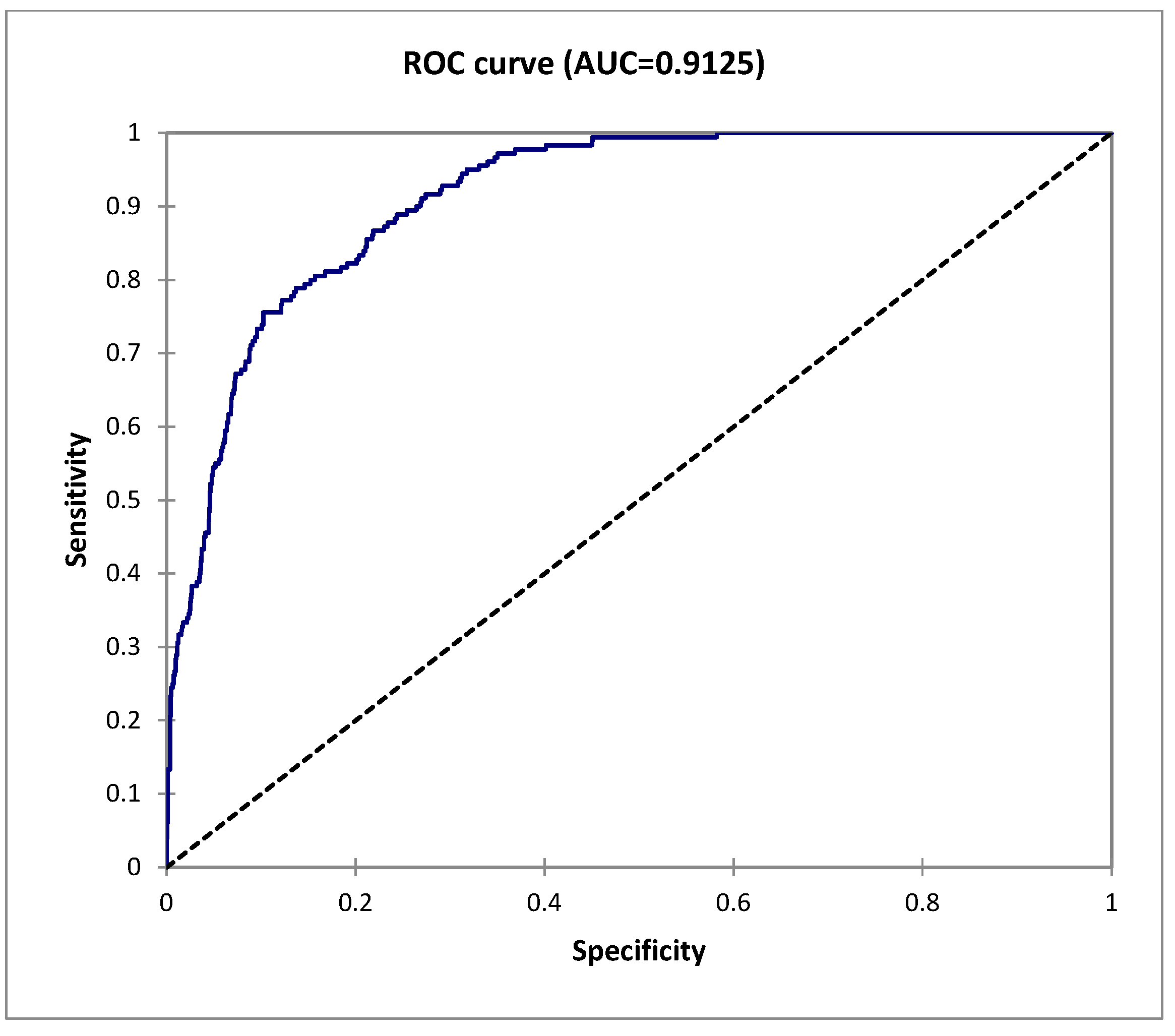
The predictive accuracy was further strongly supported by the Receiver Operating Characteristic (ROC) analysis, which yielded an Area Under the Curve (AUC) of 0.9125.

This value indicates an excellent discriminatory power of the model to distinguish between landslide and non-landslide occurrences (Figure 4).

3.2. Statistical Analysis of Decision Trees QUEST (Quick, Unbiased, Efficient Statistical Tree)

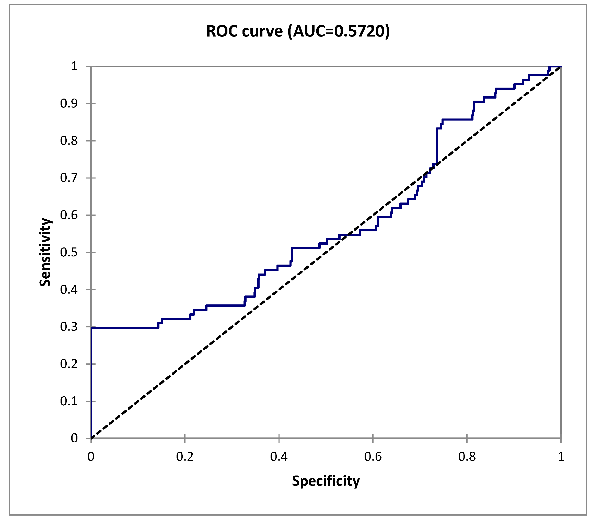
The QUEST classification algorithm identified maximum daily precipitation as the primary splitting variable, followed by lithology. This result underscores the predominant role of rainfall intensity in initiating slope failures, with geological substrate acting as a secondary susceptibility discriminator. The tree, pruned to a maximum depth of 10 using a 5% significance level, reveals a consistent decision pattern where specific precipitation thresholds, contingent on lithological class, determine the probability of landslide occurrence. Evaluation of the training dataset revealed a high overall accuracy of 91.56%. However, this metric is misleading, as it is heavily inflated by the model’s perfect specificity (100% correct classification of non-landslide cases). In contrast, the model’s sensitivity was markedly low, correctly identifying only 29.76% of actual landslide events (25 out of 84). This performance asymmetry reflects the substantial class imbalance in the dataset, where non-landslide observations constitute approximately 88% of the sample, biasing the model towards the majority class. This pattern was corroborated by the validation dataset. While overall accuracy remained high (90.67%) and specificity was perfect, the model exhibited virtually no predictive power for landslides, achieving a sensitivity of only 6.67% (2 out of 30). Consequently, the receiver operating characteristic (ROC) curve produced an area under the curve (AUC) of 0.572, indicating discriminatory performance barely superior to random chance (Figure 5).

These results indicate that while the QUEST model effectively delineates stable slopes with high reliability, its capacity to discriminate actual landslide occurrences remains limited. This shortfall is attributable primarily to the pronounced class imbalance in the dataset, which constrains the model’s ability to learn the characteristic patterns of a rare event. Consequently, although the derived decision rules are interpretable and geomorphologically sound, the model in its current form is insufficient for standalone predictive application. Its utility would require augmentation through data balancing techniques or integration with complementary analytical approaches.

3.3. Comparison QUEST-BLR

A comparative analysis of the refined Binary Logistic Regression (BLR) and QUEST algorithms reveals a critical trade-off between interpretability and predictive power for landslide susceptibility modeling, with BLR demonstrating clear overall superiority for this specific application. The primary strength of the QUEST model lies in its high interpretability. Applied to a subset of the 2011 event data, it produced a transparent, rule-based structure that is intuitively appealing for geomorphological inference. The algorithm identified maximum daily precipitation as the primary splitting variable, followed by lithology, establishing clear decision thresholds. For instance, it classified all locations receiving more than 68.6 mm of precipitation as landslide-prone. This hierarchical framework offers straightforward, rule-of-thumb insights into the primary triggers of slope failure. However, this interpretability was achieved at a severe cost to predictive performance, particularly for the critical task of identifying landslides. The QUEST model’s performance was fundamentally compromised by the pronounced class imbalance in the dataset. It exhibited a pronounced inability to generalize landslide occurrences, as evidenced by a critically low sensitivity of only 6.67% on the validation set, correctly identifying just 2 out of 30 instances. Its high overall accuracy (90.67%) was a misleading metric, driven entirely by perfect specificity (100% correct classification of stable slopes). The resulting Area Under the Curve (AUC) of 0.572 signifies a discriminatory capacity barely superior to random chance, rendering it operationally unsuitable for early warning systems. In stark contrast, the refined BLR model demonstrated a robust balance of interpretability, statistical rigor, and high predictive accuracy. While its parameter coefficients are less immediately intuitive than a decision tree, the model provides a probabilistic framework that is both geomorphologically sound and statistically reliable. More importantly, the BLR model successfully overcame the limitations posed by class imbalance that crippled the QUEST algorithm. It maintained a very strong and well-calibrated predictive performance, with an AUC of 0.913 on the estimation data and a consistent overall accuracy of 80.33% on an independent validation sample. Crucially, it achieved this without sacrificing its ability to identify landslide events, demonstrating balanced sensitivity (81.11%) and specificity (82.21%). This balance is paramount for a predictive tool, as both false alarms and missed alarms carry significant consequences. In conclusion, while the QUEST model offers valuable insights into the hierarchical structure of landslide triggers, its practical utility was severely constrained in this dataset by the pronounced class imbalance between landslide and non-landslide observations, to which single decision trees are known to be particularly sensitive [19,37]. The BLR model, by contrast, demonstrated a robust capacity to handle this imbalance natively, modelling minority-class probabilities directly through the logistic link function without requiring preprocessing of the training data. This represents a genuine practical advantage in operational landslide monitoring contexts, where imbalanced observations are the rule rather than the exception. On this basis, the BLR model was selected as the reference framework for the development of the susceptibility, hazard, and threshold maps presented in this study. It should be noted, however, that the comparison presented here reflects unprocessed data conditions and that the application of data-balancing techniques, such as SMOTE oversampling or cost-sensitive learning to the QUEST algorithm was not pursued in this study. Such approaches could potentially narrow the observed performance gap by improving the sensitivity of the decision tree to the minority (landslide) class, and their evaluation is recommended as a direction for future research.

3.4. Interpretation and Physical Meaning of Parameters Based on Statistical Results

In a multivariate BLR, the interpretation of individual predictor thresholds is not straightforward, as the effect of each variable depends on the values of the others. Rather than a single universal threshold, the contribution of each predictor must be evaluated within the context of the entire feature set. The following analysis summarizes the direction, significance, and relative influence of the key predictors in the refined model (

Table 5. Summary of Key Predictor Effects Across Landslide Models.

Predictor	Unified Model	Interpretation of Effect
Rainfall Intensity	β = +0.026 (p < 0.0001) OR = 1.03	A significant trigger. Each 1 mm increase in intensity increases the odds of failure by 2.6%.
Slope (16–25°)	β = −2.872 (p < 0.0001) OR = 0.06	The most consistent stabilizing factor. This class has 94.3% lower odds of failure compared to the 0–16° reference class.
Lithology (Clays)	β = +1.796 (p < 0.0001) OR = 6.03	The paramount risk factor. Presence of this lithology increases the odds of failure by over 6 times compared to deposits.
Aspect (Southeast)	β = −2.498 (p = 0.0002) OR = 0.08	Southeast-facing slopes are associated with a drastic (91.8%) reduction in risk compared to South-facing slopes.

β: Coefficient; OR: Odds Ratio (effect size); p: p-value (statistical significance). Reference categories are: Slope (0–16°), Lithology (Deposits), Aspect (South/Northwest).

).

The refined BLR model provides a robust and stable framework for landslide prediction. It establishes a clear hierarchy of predictive factors, in which geological predisposition sets the baseline conditions, topography delineates the spatial pattern of susceptibility, and short-term hydrological inputs act as the primary dynamic triggers. Among the predictors, Lithology emerges as the most powerful and consistent factor (Table 5). Specifically, the presence of clays and marly clays with intercalations of sandstones, sands, and conglomerates is associated with a substantial increase in landslide risk (OR = 6.03), confirming that this clay-rich formation represents the primary perennial risk factor in the region. Slope gradient constitutes the most significant stabilizing topographic factor. The model strongly reinforces that the 0–16° slope class corresponds to the highest susceptibility, while the 16–25° class exerts a marked stabilizing effect (OR = 0.057). This supports the interpretation that the dominant failure mechanisms are shallow translational slides and flows, which preferentially initiate on gentler slopes. This apparently counterintuitive result, whereby the lowest slope class shows the highest susceptibility, is well-documented in the Italian Apennine context and can be explained by two concurring physical mechanisms. First, clay-rich soils on gentle slopes accumulate thicker colluvial and weathering mantles, as deposition prevails over erosion; this greater thickness of unstable material directly increases the potential volume of failure for translational slides and earth flows. Second, low-gradient clay soils retain infiltrating water more effectively, promoting the build-up of pore-water pressure during intense precipitation events, the primary trigger identified by the model. On steeper slopes (16–25°), the soil mantle is typically thinner and bedrock or coarser material is more frequently exposed, reducing both the available failure volume and the capacity for hydrological accumulation. This interpretation is consistent with evidence from the IFFI database (Inventario dei Fenomeni Franosi in Italia), which documents that translational slides and earth flows in the central Apennines preferentially initiate on slope angles between 5° and 20°, with relatively few events recorded on slopes exceeding 25° in clay-dominated terrains [2]. Among hydrological drivers, maximum daily precipitation intensity retains its role as a significant positive trigger. The odds ratio indicates that for each additional millimeter of peak rainfall intensity, the likelihood of a landslide increases by 2.6%, conditional on the other variables (Table 5). This factor also represents the most practical input for operational early warning systems. The logical and physical connections among these retained predictors are not incidental but reflect a coherent, multi-stage failure mechanism. Lithology sets the baseline susceptibility by controlling soil composition, permeability, and mechanical strength: clay-rich units with interbedded sands and conglomerates create the primary predisposing condition through their low shear strength and high plasticity. Slope gradient, rather than acting independently, interacts directly with lithological thickness. In this clay-dominated landscape, gentler slopes accumulate thicker colluvial mantles because depositional processes prevail over erosion, so that the lowest slope class (0–16°) paradoxically concentrates the greatest volume of unstable material and the highest capacity for pore-water pressure build-up. Maximum daily precipitation then acts as the immediate dynamic trigger: by rapidly infiltrating fine-grained, partially saturated soils it elevates pore-water pressure, reducing effective normal stress and pushing the slope past the failure threshold set by the lithological and topographic conditions already in place. Land use modulates this hydrological response by controlling surface infiltration rates and root reinforcement, while slope aspect governs the solar radiation budget and evapotranspiration regime, together determining the antecedent moisture state of the soil before a triggering event. Southeast-facing slopes, which receive intense direct solar radiation, show markedly lower failure odds (OR = 0.08), consistent with higher evapotranspiration and therefore lower antecedent saturation compared to south- or northwest-facing slopes. The multivariate BLR framework captures precisely this cascade: predisposition (lithology); structural amplification (slope gradient × colluvial thickness); hydrological modulation (land use, aspect); dynamic triggering (precipitation intensity), such that the probability of failure at any location reflects the combined state of all these interacting controls. The high predictive performance of the model (AUC > 0.91) demonstrates that, although individual events exhibit unique characteristics, landslide occurrence follows a stable and statistically modelable process framework. These findings are consistent with the validation results reported in Section 3.1, where the refined BLR model achieved an AUC of 0.913 on the independent validation sample (Table 4, Figure 4), confirming its strong discriminatory performance. Furthermore, the identified controlling factors—clay-rich lithology, gentle slope gradients (0–16°), and maximum daily precipitation intensity—align with independent susceptibility assessments conducted for adjacent areas in the central Apennines. Studies in the Marche and Umbria regions have similarly identified clay lithology and rainfall intensity as primary landslide predisposing and triggering factors [2,5], providing additional geomorphological corroboration of the model’s outputs. By addressing multicollinearity, the refined model offers the most robust tool for regional landslide susceptibility assessment, capturing the core mechanics of failure across diverse triggering conditions with enhanced statistical stability. The final probability of landslide occurrence is derived from the combined influence of these variables through the logistic function. The equation of the refined model is:

$$\mathrm{l}\mathrm{o}\mathrm{g}\mathrm{i}\mathrm{t}\left(\mathrm{p}\right)=\mathsf{\beta }0+\mathsf{\beta }1\cdot \mathrm{p}\_07032008+\mathsf{\beta }2\cdot \mathrm{C}\mathrm{L}\mathrm{C}+\mathsf{\beta }3\cdot \mathrm{S}\mathrm{l}\mathrm{o}\mathrm{p}\mathrm{e}+\mathsf{\beta }4\cdot \mathrm{L}\mathrm{i}\mathrm{t}\mathrm{h}\mathrm{o}\mathrm{l}\mathrm{o}\mathrm{g}\mathrm{y}+\mathsf{\beta }5\cdot \mathrm{A}\mathrm{s}\mathrm{p}\mathrm{e}\mathrm{c}\mathrm{t}$$

(12)

Equation (12) can be directly implemented in a GIS environment to generate landslide probability maps for land-use planning and hazard mitigation (13), by applying the logistic transformation:

$$\mathrm{p}={\displaystyle \frac{1}{1+\mathrm{e}-\mathrm{l}\mathrm{o}\mathrm{g}\mathrm{i}\mathrm{t}\left(\mathrm{p}\right)}}$$

(13)

3.5. Susceptibility, Hazard, and Activation Thresholds for the Study Area

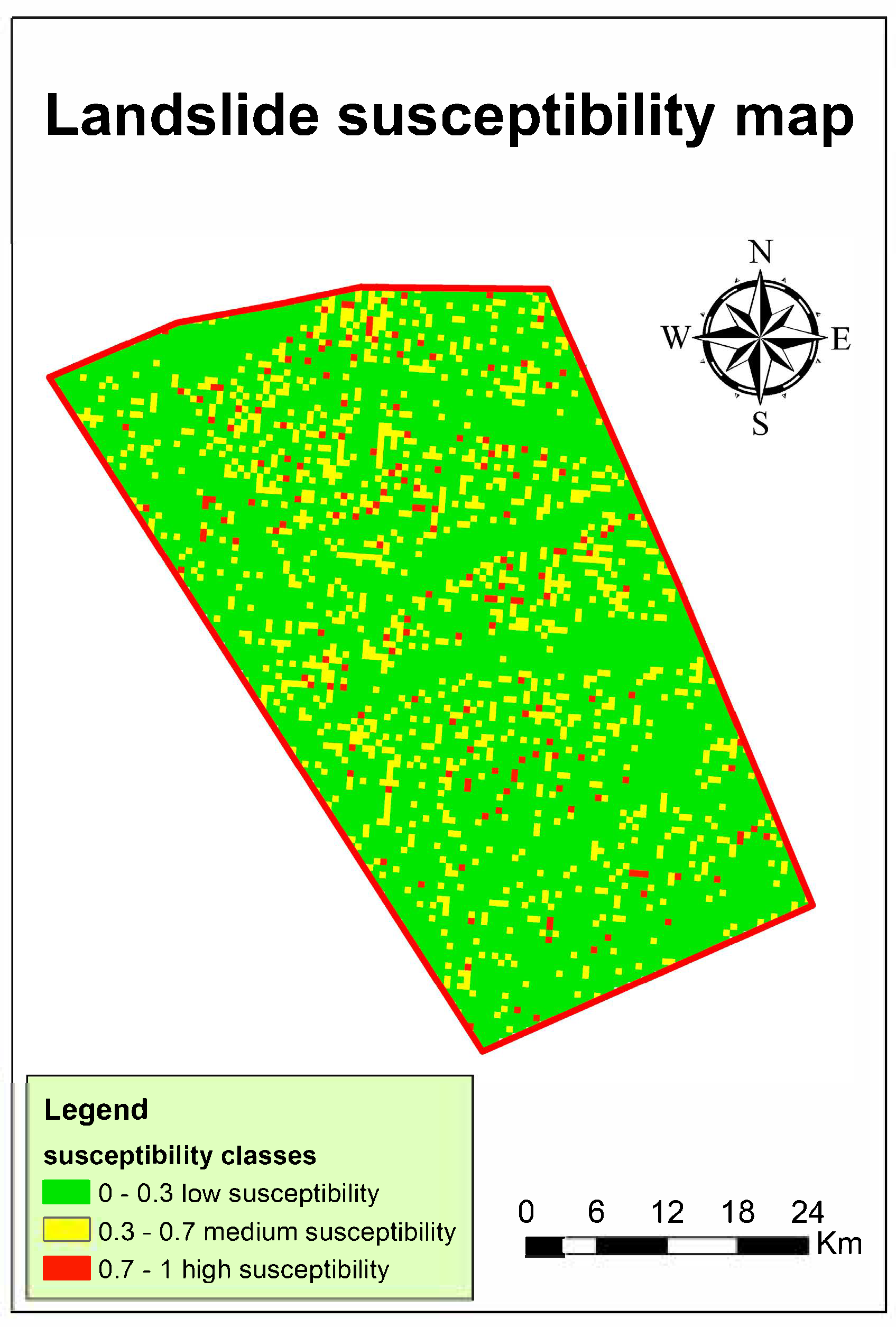
In this study, probability thresholds were not arbitrarily selected but derived from the statistical performance of the logistic regression model. The continuous probability output (ranging from 0 to 1) was evaluated against the landslide inventory using receiver operating characteristic (ROC) analysis, from which sensitivity, specificity, and Youden’s J statistic were calculated for all possible cut-off values. The high-probability class was defined for values exceeding 0.70, corresponding to the threshold that maximized Youden’s J (J = Sensitivity + Specificity − 1). This cut-off represents the optimal trade-off between correctly identifying landslide-prone areas (true positives) and minimizing false alarms (false positives). The 0.70 threshold also coincides with the point where the cumulative distribution of predicted probabilities for landslide occurrences shows a sharp increase, further confirming its discriminative capacity. Additional verification through bootstrap resampling confirmed the stability of this threshold (95% CI ≈ 0.68–0.73). Consequently, adopting 0.70 as the threshold ensures that areas classified as “high susceptibility” correspond to locations where the model assigns a high level of confidence to the presence of landslide conditions. To convert the continuous probability surface into a categorical landslide susceptibility map, three probability classes were defined: low (p < 0.30), moderate (0.30 ≤ p < 0.70), and high (p ≥ 0.70). The thresholds were statistically derived rather than arbitrarily imposed, and their choice is consistent with methodologies reported in the literature. Specifically, the upper cut-off value of 0.70 maximizes Youden’s J statistic on the ROC curve, ensuring the best compromise between sensitivity (true positive rate) and specificity (true negative rate). This criterion guarantees that “high susceptibility” areas correspond to zones of robust model confidence, thus reducing false positives while maintaining an adequate detection of known landslides. The lower threshold (p = 0.30) was established through an analysis of the cumulative distribution of predicted probabilities, identifying the point below which more than 70% of non-landslide pixels were concentrated. This ensures that the “low susceptibility” class is associated with locations where the modeled risk is negligible. The intermediate class (0.30 ≤ p < 0.70) reflects transitional conditions, capturing the uncertainty of the model in areas where environmental factors are less conclusive. Similar approaches, using ROC-derived thresholds or cumulative probability distributions, are widely adopted in susceptibility mapping [38,39], further supporting the robustness of the classification applied here. Based on the statistical model and its integration within a GIS environment, three different map products were developed: (i) a landslide susceptibility map, (ii) a landslide hazard map, and (iii) a threshold-value map. The landslide susceptibility map highlights areas potentially prone to landslides under average rainfall triggering conditions. It was produced by conditioning the logistic regression model with the mean of annual maximum daily precipitation values for the period 1991–2020, interpolated across the study area using the Empirical Bayesian Kriging (EBK) method (Figure 6). The results show that average rainfall conditions correspond predominantly to low susceptibility, with widespread areas of medium susceptibility and more localized clusters of high susceptibility distributed throughout the study area.

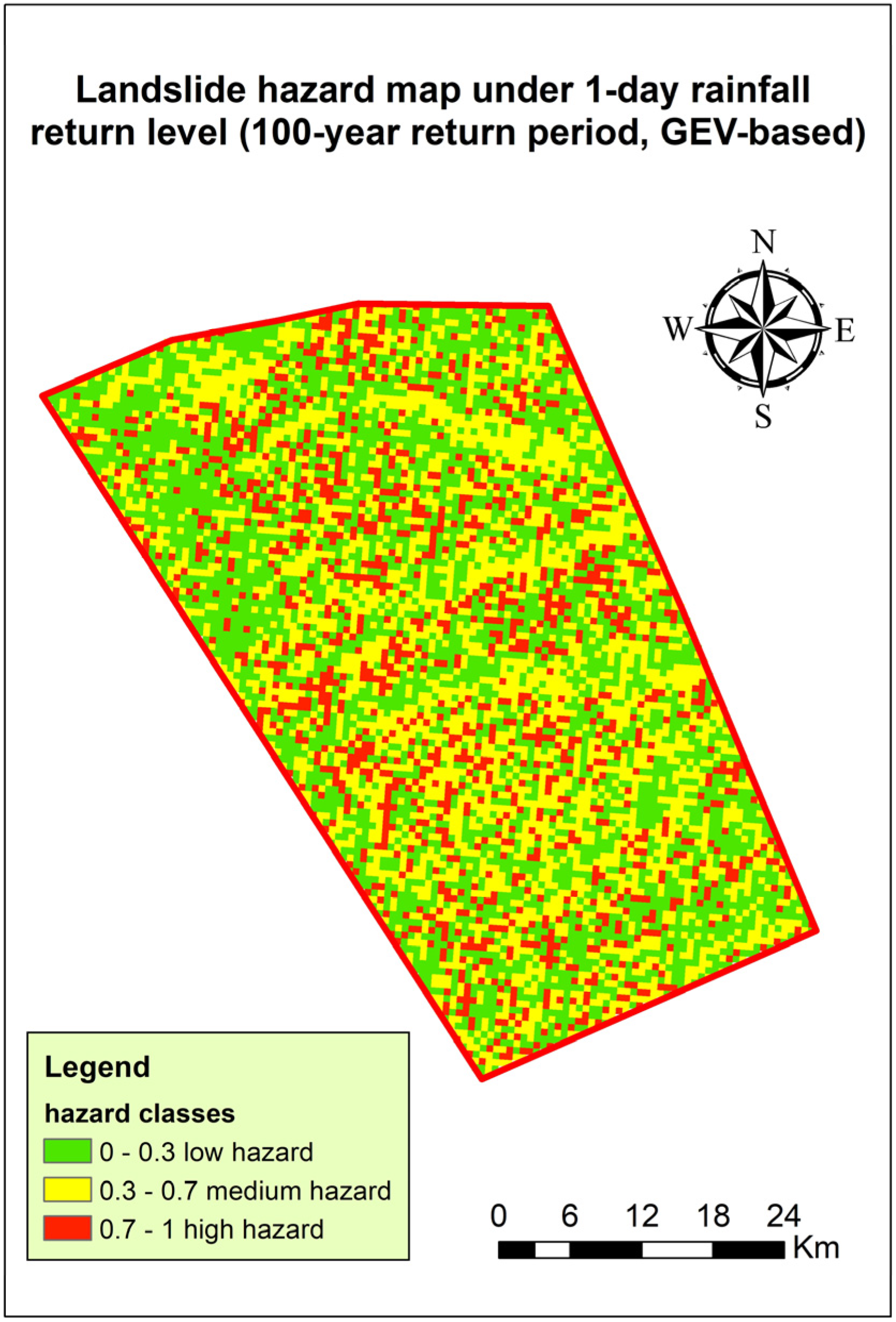
The landslide hazard map, in contrast, integrates return period information and therefore provides a temporal dimension to the assessment. It was obtained by conditioning the logistic regression model with the 1-day rainfall return level associated with a 100-year return period, estimated through Generalized Extreme Value (GEV) analysis of rain gauge data from 1991 to 2020. The interpolated values were then applied across the study area (Figure 7). This map does not only indicate areas prone to landslides but also associates them with the return period of extreme rainfall, thereby representing the likelihood of occurrence within a given time frame. Under this extreme rainfall scenario, the study area exhibits widespread medium hazard and several zones of high hazard, highlighting the increased instability expected under rare but intense precipitation events.

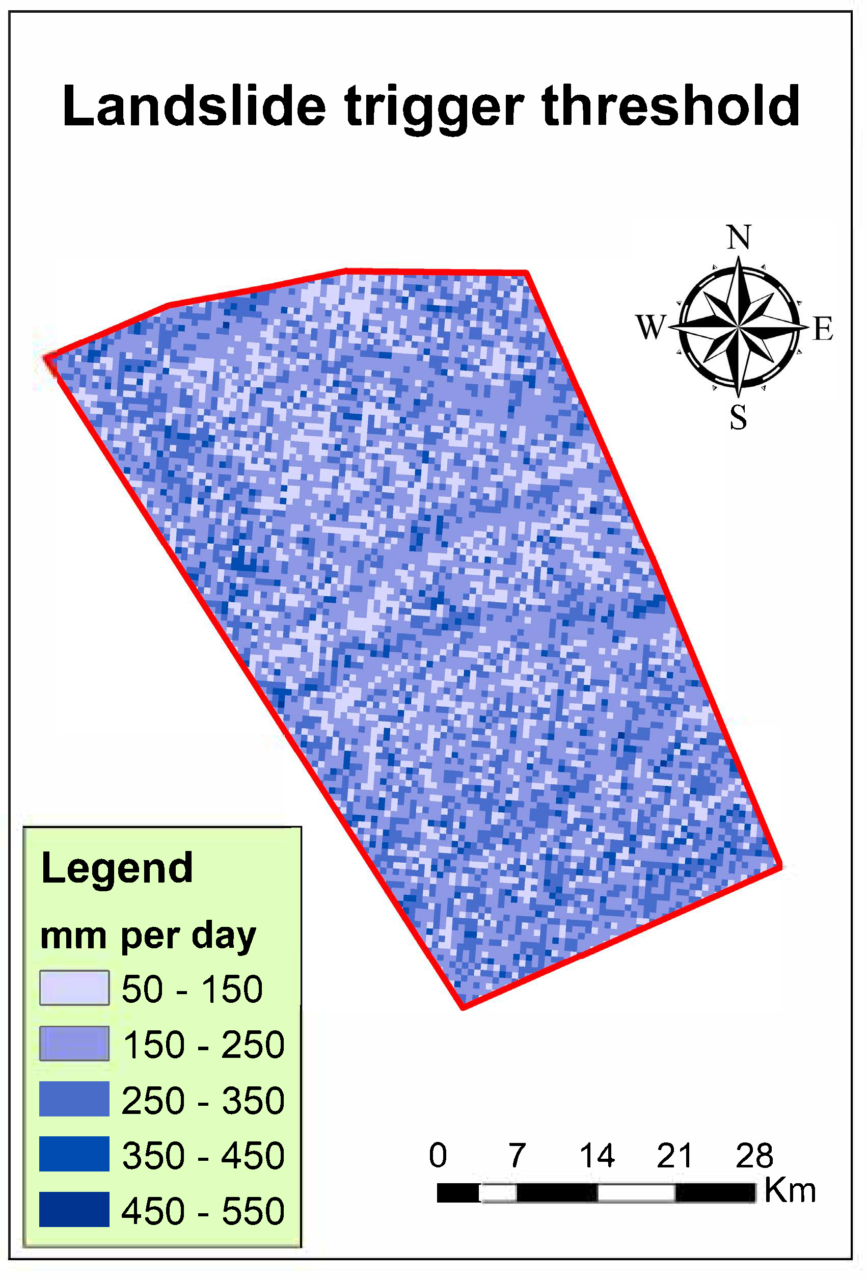
Finally, a threshold-value map was developed as a derivative product, providing a practical tool for risk management. By setting the probability level at >0.70, the model isolates the precipitation threshold (in mm) associated with landslide initiation in each location (Figure 8). This product is particularly relevant for operational applications, as it provides easily interpretable data suitable for real-time alert systems.

The spatial distribution of thresholds indicates that in many parts of the study area, landslides are likely to be triggered only when daily rainfall exceeds 100 mm (Figure 8). Thus, this map represents a direct linkage between probability modeling and rainfall-based triggering thresholds, bridging the gap between statistical analysis and practical early-warning applications. To verify the spatial consistency of the threshold-value map against observed triggering conditions, a retrospective check was performed for the three calibration events. For each event, the observed maximum daily precipitation recorded at the nearest rain gauge was compared with the locally predicted threshold at each mapped landslide location. For the March 2010 event, which recorded the highest rainfall intensities among the three, the observed precipitation exceeded the model-predicted threshold in approximately 87% of landslide locations, confirming a high degree of spatial agreement between the threshold map and actual triggering conditions. Similar consistency was observed for the 2008 and 2011 events. It should be noted that, since these events were used in model calibration, this represents an internal retrospective verification rather than a fully independent validation; a rigorous independent test against future or withheld events remains an important objective for future research. Taken together, these three products provide complementary perspectives on landslide risk: the susceptibility map delineates spatial predisposition under average conditions, the hazard map integrates frequency and intensity of extreme rainfall events, and the threshold-value map translates probability outputs into actionable rainfall triggers. This integrated framework strengthens the interpretability and practical relevance of susceptibility modeling for both scientific research and decision-making in landslide risk management.

4. Discussion

The findings of this study contribute to the ongoing discourse in landslide modeling by demonstrating that a rigorously refined Binary Logistic Regression (BLR) framework can achieve superior and more stable performance compared to a tree-based algorithm like QUEST for event-based landslide prediction, particularly when dealing with the inherent imbalance between landslide and non-landslide observations. This outcome provides a nuanced counterpoint to the prevailing trend in the literature that often champions complex machine learning (ML) models like Random Forest for their superior predictive power [17,40,41]. Our results align, instead, with a body of work affirming the competitiveness of well-specified parametric models, especially when interpretability, statistical rigor, and operational stability are paramount [42,43,44]. The decision not to include Random Forest or other ensemble methods in the primary comparison was deliberate. This study prioritizes interpretability and direct operational applicability—specifically, the ability to invert the model equation to derive spatially distributed rainfall thresholds across the landscape. Ensemble methods, while often superior in raw predictive accuracy, do not yield an explicit parametric equation amenable to this inversion, and their opacity conflicts with the transparency required for civil protection decision-making. The BLR–QUEST comparison was therefore designed to contrast a parametric probabilistic model with the most interpretable tree-based alternative, framing the choice not as a benchmark across all available algorithms but as a methodologically justified selection aligned with the operational objectives of the study. The failure of the QUEST algorithm, which exhibited high specificity but critically low sensitivity (6.67%), underscores a known vulnerability of single decision trees to severe class imbalance, often leading to poor generalization for the minority class [15,19,37]. In contrast, the BLR’s balanced performance, achieved through careful variable selection to mitigate multicollinearity, highlights that model parsimony can be a strength, not a limitation, in scenarios where predictor interactions are not overwhelmingly complex [45]. The core innovation of this analysis, however, extends beyond model selection. By calibrating the model exclusively on landslides with known activation dates from multiple extreme events, this research firmly embeds itself within the emerging paradigm of event-based susceptibility mapping [9,46]. This approach moves beyond static, inventory-driven susceptibility models, which amalgamate landslides of different ages and triggers, to model the conditional probability of failure given a specific precipitation trigger. Our methodology thus directly addresses the call for more dynamic hazard assessments that integrate time-variable triggering factors, as advocated by Segoni et al. (2018) [7] and Ng et al. (2021) [47]. Unlike traditional susceptibility maps that answer “where” landslides might occur, our event-based framework begins to answer “when” and “under what conditions,” providing a more direct link to early warning. The most significant advancement lies in the integrated workflow that derives three distinct products from a single calibrated model. This multi-faceted output strategy is analogous to the dynamic approach proposed by Segoni et al. (2018) [7], who combined rainfall thresholds with susceptibility maps. However, our study advances this concept by fully integrating the triggering variable (precipitation) directly into the susceptibility model itself. The resulting products, a susceptibility map conditioned on average extreme rainfall, a hazard map for a 100-year return period scenario, and a novel spatially distributed map of activation thresholds, offer a comprehensive toolkit for risk management [48]. This latter product, generated by inverting the logistic equation to solve for the precipitation required to exceed a critical probability threshold (p > 0.7) across the landscape, represents a substantive leap beyond regional empirical threshold curves [38]. It provides a directly actionable tool for early warning systems by explicitly answering the critical question of “how much rain is needed where”, thereby spatializing the concept of a triggering threshold in a way that acknowledges the modulating role of local lithology, slope, and land use. This moves operational practice from a single threshold for a large region towards a spatially variable field of thresholds, enhancing precision and potentially reducing false alarms. Furthermore, the geomorphological consistency of our BLR model reinforces its physical plausibility. The identification of clay-rich lithologies as the paramount predisposing factor and gentler slopes (0–16°) as most susceptible is well-documented in the Apennine context [2,6,49] and aligns with the dominance of shallow, translational slides and earth flows in such terrains. This consistency with established geological understanding bolsters confidence in the model’s transferability and its value for land-use planning, complementing its predictive accuracy. Overall this study demonstrates that a carefully constructed BLR model is not only competitive with but can surpass more complex ML techniques for event-based landslide prediction, particularly when data imbalance and interpretability are key concerns. By championing an event-based, multi-output approach, it provides a replicable framework for developing dynamic, operationally relevant landslide hazard assessments that effectively bridge the gap between academic research and the practical needs of disaster risk reduction.

Limitations

Several limitations of this study should be acknowledged. First, the analysis is confined to a single pilot area in central Italy, with specific lithological, climatic, and morphological characteristics. Although the methodology is designed to be transferable, the model coefficients and derived thresholds are calibrated on local data and require recalibration before application to other regions. Second, the event-based calibration relies on three extreme precipitation episodes (2008, 2010, and 2011), all occurring during the late-winter season. This temporal homogeneity strengthens internal consistency, but the calibrated thresholds may not fully capture triggering conditions associated with summer convective storms or prolonged autumnal rainfall, which involve different antecedent soil moisture dynamics. Future work should extend the event database to a broader range of seasonal conditions and validate the methodology in geologically and climatically distinct regions. Finally the soil saturation estimates derived from the [34] pedotransfer functions could not be validated against in situ measurements, given the absence of a sufficiently dense field monitoring network in the study area. Moreover, the 15-day antecedent window, while physically justified for clay-rich soils, was not tested against alternative time scales (7-day, 30-day). Sensitivity analyses on this parameter, as well as comparisons across different lithological contexts, represent a worthwhile avenue for future research. It should be noted, however, that soil saturation was ultimately excluded from the final predictive model due to multicollinearity, limiting the practical impact of these uncertainties on the study’s conclusions

5. Conclusions

This study successfully developed and validated a robust, event-based landslide prediction framework for a high-risk area in central Italy. The core methodological finding is that a carefully refined Binary Logistic Regression (BLR) model outperformed the QUEST decision tree algorithm, achieving excellent predictive accuracy (AUC = 0.913) and stability, particularly in handling imbalanced landslide data. The model identified a clear hierarchy of controlling factors, with clay-rich lithology as the primary predisposing condition, gentle to moderate slopes (0–16°) as the most susceptible class, and maximum daily precipitation intensity as the critical dynamic trigger. These findings carry clear geological significance. The dominance of clay-rich lithology (OR = 6.03) reflects the well-known mechanical behaviour of pelitic formations in the central Apennines: their low shear strength, high plasticity, and pronounced shrink–swell response create perennially unstable conditions that precipitation alone is sufficient to trigger into failure. The counterintuitive susceptibility pattern on gentle slopes (0–16°) is physically coherent in this context, as thicker colluvial mantles accumulate on low-gradient clay terrain where deposition prevails over erosion, providing both greater failure volume and enhanced capacity for pore-water pressure build-up. The superiority of BLR over QUEST in this setting is itself methodologically interpretable: it reflects the fact that landslide occurrence in imbalanced datasets is better modelled through a parametric probabilistic framework that directly estimates minority-class probabilities, rather than through rule-based splitting that is structurally biased towards the majority class. The principal innovation of this research lies in its integrated, multi-output workflow that advances beyond conventional static susceptibility mapping. By calibrating the model on landslides with known activation dates from multiple extreme events, we generated three distinct and operationally valuable products from a single statistical core:

• A Dynamic Susceptibility Map: Conditioning the model on average annual maximum rainfall provides a realistic baseline of landslide probability.
• A Scenario-Based Hazard Map: Using the 100-year return period rainfall transforms the susceptibility model into a temporal hazard assessment for extreme events.
• A Spatially Distributed Threshold Map: This novel product inverts the model to pinpoint the specific rainfall intensity required to exceed a critical probability threshold (p > 0.7) at any location. This effectively spatializes empirical thresholds, moving from a regional “if-then” curve to a localized “how much rain, and where” guidance system.

In conclusion, this research provides a replicable methodology that effectively bridges the gap between statistical landslide modeling and practical risk management. The demonstrated superiority of a parsimonious BLR model underscores that interpretability and statistical robustness can coexist with high predictive performance. The derived maps, especially the spatially explicit activation thresholds, offer a directly actionable tool for land-use planning, civil protection, and the development of next-generation, location-specific early warning systems. Crucially, the threshold map represents a conceptual advance over traditional regional empirical curves: rather than issuing a single rainfall threshold for an entire administrative area, it provides a spatially variable field of thresholds that explicitly accounts for the modulating role of local lithology, slope gradient, and land use, thereby acknowledging that the same rainfall intensity may be harmless in one location and triggering in another only metres away. It should be noted, however, that the derived thresholds are currently season-specific, calibrated exclusively on late-winter events characterized by high antecedent soil moisture and prolonged rainfall; their applicability to summer convective or autumnal rainfall scenarios requires further validation.

References

1. Wu, X.; Chen, X.; Zhan, F.B.; Hong, S. Global research trends in landslides during 1991–2014: A bibliometric analysis. Landslides 2015, 12, 1215–1226. [Google Scholar] [CrossRef]
2. Trigila, A.; Iadanza, C.; Guerrieri, L.; Hervás, J. The IFFI project (Italian landslide inventory): Methodology and results. Guidel. Mapp. Areas Risk Landslides Eur. 2007, 23, 15. [Google Scholar]
3. Trigila, A.; Iadanza, C.; Bussettini, M.; Mariani, S.; D’Ascola, F.; Salmeri, A.; Cassese, M.L.; Pesarino, V.; Di Paola, G.; Romeo, S.; et al. Dissesto idrogeologico in Italia: Pericolosità e indicatori di rischio: Edizione 2024. Rapporto 2025, 415, 2025. [Google Scholar]
4. Handwerger, A.L.; Huang, M.H.; Fielding, E.J.; Booth, A.M.; Bürgmann, R. A shift from drought to extreme rainfall drives a stable landslide to catastrophic failure. Sci. Rep. 2019, 9, 1569. [Google Scholar] [CrossRef]
5. Gentilucci, M.; Materazzi, M.; Pambianchi, G. Statistical analysis of landslide susceptibility, Macerata province (Central Italy). Hydrology 2021, 8, 5. [Google Scholar] [CrossRef]
6. Gentilucci, M.; Pelagagge, N.; Rossi, A.; Domenico, A.; Pambianchi, G. Landslide susceptibility using climatic–environmental factors using the weight-of-evidence method—A study area in Central Italy. Appl. Sci. 2023, 13, 8617. [Google Scholar] [CrossRef]
7. Segoni, S.; Tofani, V.; Rosi, A.; Catani, F.; Casagli, N. Combination of rainfall thresholds and susceptibility maps for dynamic landslide hazard assessment at regional scale. Front. Earth Sci. 2018, 6, 85. [Google Scholar] [CrossRef]
8. Liu, Q.; Zhao, Q.; Lan, Q.; Huang, C.; Yang, X.; Tang, Z.; Deng, M. Regional dynamic hazard assessment of rainfall–induced landslide guided by geographic similarity. Bull. Eng. Geol. Environ. 2024, 83, 501. [Google Scholar] [CrossRef]
9. Bhandary, N.P.; Dahal, R.K.; Timilsina, M.; Yatabe, R. Rainfall event-based landslide susceptibility zonation mapping. Nat. Hazards 2013, 69, 365–388. [Google Scholar] [CrossRef]
10. Antonetti, G.; Gentilucci, M.; Aringoli, D.; Pambianchi, G. Analysis of landslide susceptibility and tree felling due to an extreme event at mid-latitudes: Case study of Storm Vaia, Italy. Land 2022, 11, 1808. [Google Scholar] [CrossRef]
11. Shahabi, H.; Rahimzad, M.; Tavakkoli Piralilou, S.; Ghorbanzadeh, O.; Homayouni, S.; Blaschke, T.; Lim, S.; Ghamisi, P. Unsupervised deep learning for landslide detection from multispectral sentinel-2 imagery. Remote Sens. 2021, 13, 4698. [Google Scholar] [CrossRef]
12. Zhang, X.; Pun, M.O.; Liu, M. Semi-supervised multi-temporal deep representation fusion network for landslide mapping from aerial orthophotos. Remote Sens. 2021, 13, 548. [Google Scholar] [CrossRef]
13. Chrysafi, A.A.; Tsangaratos, P.; Ilia, I.; Chen, W. Rapid Landslide Detection Following an Extreme Rainfall Event Using Remote Sensing Indices, Synthetic Aperture Radar Imagery, and Probabilistic Methods. Land 2024, 14, 21. [Google Scholar] [CrossRef]
14. Ayalew, L.; Yamagishi, H. The application of GIS-based logistic regression for landslide susceptibility mapping in the Kakuda-Yahiko Mountains, Central Japan. Geomorphology 2005, 65, 15–31. [Google Scholar] [CrossRef]
15. Alkhasawneh, M.S.; Ngah, U.K.; Tay, L.T.; Mat Isa, N.A.; Al-Batah, M.S. Modeling and testing landslide hazard using decision tree. J. Appl. Math. 2014, 2014, 929768. [Google Scholar] [CrossRef]
16. Sun, D.; Wen, H.; Wang, D.; Xu, J. A random forest model of landslide susceptibility mapping based on hyperparameter optimization using Bayes algorithm. Geomorphology 2020, 362, 107201. [Google Scholar] [CrossRef]
17. Yao, J.; Yao, X.; Zhao, Z.; Liu, X. Performance comparison of landslide susceptibility mapping under multiple machine-learning based models considering InSAR deformation: A case study of the upper Jinsha River. Geomat. Nat. Hazards Risk 2023, 14, 2212833. [Google Scholar] [CrossRef]
18. Nhu, V.H.; Mohammadi, A.; Shahabi, H.; Ahmad, B.B.; Al-Ansari, N.; Shirzadi, A.; Geertsema, M.; Kress, V.R.; Karimzadeh, S.; Valizadeh Kamran, K.; et al. Landslide detection and susceptibility modeling on cameron highlands (Malaysia): A comparison between random forest, logistic regression and logistic model tree algorithms. Forests 2020, 11, 830. [Google Scholar] [CrossRef]
19. Perlich, C.; Provost, F.; Simonoff, J.S. Tree induction vs. logistic regression: A learning-curve analysis. J. Mach. Learn. Res. 2003, 4, 211–255. [Google Scholar]
20. Kirasich, K.; Smith, T.; Sadler, B. Random forest vs logistic regression: Binary classification for heterogeneous datasets. SMU Data Sci. Rev. 2018, 1, 9. [Google Scholar]
21. Couronné, R.; Probst, P.; Boulesteix, A.L. Random forest versus logistic regression: A large-scale benchmark experiment. BMC Bioinform. 2018, 19, 270. [Google Scholar] [CrossRef] [PubMed]
22. Forkuor, G.; Hounkpatin, O.K.; Welp, G.; Thiel, M. High resolution mapping of soil properties using remote sensing variables in south-western Burkina Faso: A comparison of machine learning and multiple linear regression models. PLoS ONE 2017, 12, e0170478. [Google Scholar] [CrossRef] [PubMed]
23. Halder, K.; Srivastava, A.K.; Ghosh, A.; Das, S.; Banerjee, S.; Pal, S.C.; Chatterjee, U.; Bisai, D.; Ewert, F.; Gaiser, T. Improving landslide susceptibility prediction through ensemble recursive feature elimination and meta-learning framework. Sci. Rep. 2025, 15, 5170. [Google Scholar] [CrossRef] [PubMed]
24. Evangelia, C.; Jie, M.; Collins, G.; Steyerberg, E.; Verbakel, J.; Van Calster, B. A systematic review shows no performance benefit of machine learning over logistic regression for clinical prediction models. J. Clin. Epidemiol. 2019, 110, 12–22. [Google Scholar]
25. Gentilucci, M.; Barbieri, M.; Burt, P. Climate and territorial suitability for the Vineyards developed using GIS techniques. In Conference of the Arabian Journal of Geosciences; Springer International Publishing: Cham, Switzerland, 2018; pp. 11–13. [Google Scholar]
26. Hosmer, D.W.; Lemeshow, S. Applied Logistic Regression; Wiley: New York, NY, USA, 2000. [Google Scholar]
27. Gentilucci, M.; Pambianchi, G. Prediction of snowmelt days using binary logistic regression in the Umbria-Marche apennines (Central Italy). Water 2022, 14, 1495. [Google Scholar] [CrossRef]
28. Loh, W.Y.; Shih, Y.S. Split selection methods for classification trees. Stat. Sin. 1997, 7, 815–840. [Google Scholar]
29. Gentilucci, M.; Rossi, A.; Pelagagge, N.; Aringoli, D.; Barbieri, M.; Pambianchi, G. GEV analysis of extreme rainfall: Comparing different time intervals to analyse model response in terms of return levels in the study area of central Italy. Sustainability 2023, 15, 11656. [Google Scholar] [CrossRef]
30. Gentilucci, M.; Barbieri, M.; Younes, H.; Rihab, H.; Pambianchi, G. Analysis of Wildfire Susceptibility by Weight of Evidence, Using Geomorphological and Environmental Factors in the Marche Region, Central Italy. Geosciences 2024, 14, 112. [Google Scholar] [CrossRef]
31. R Core Team. R: A Language and Environment for Statistical Computing; R Foundation for Statistical Computing: Vienna, Austria, 2025; Available online: https://www.R-project.org/ (accessed on 12 December 2025).
32. Gentilucci, M.; Djouohou, S.I.; Barbieri, M.; Hamed, Y.; Pambianchi, G. Trend analysis of streamflows in relation to precipitation: A case study in Central Italy. Water 2023, 15, 1586. [Google Scholar] [CrossRef]
33. European Soil Data Centre (ESDAC). European Soil Data Centre: Soil Data and Information Systems; Joint Research Centre, European Commission: Brussels, Belgium, 2023; Available online: https://esdac.jrc.ec.europa.eu/ (accessed on 25 January 2025).
34. Cosby, B.J.; Hornberger, G.M.; Clapp, R.B.; Ginn, T.R. A statistical exploration of the relationships of soil moisture characteristics to the physical properties of soils. Water Resour. Res. 1984, 20, 682–690. [Google Scholar] [CrossRef]
35. Rawls, W.J.; Brakensiek, D.L.; Saxton, K.E. Estimation of soil water properties. Trans. ASAE 1982, 25, 1316–1320. [Google Scholar] [CrossRef]
36. Allen, R.G.; Pereira, L.S.; Raes, D.; Smith, M. Crop Evapotranspiration–Guidelines for Computing Crop Water Requirements (FAO Irrigation and Drainage Paper No. 56); Food and Agriculture Organization of the United Nations: Rome, Italy, 1998. [Google Scholar]
37. Fu, Z.; Ma, H.; Wang, F.; Dou, J.; Zhang, B.; Fang, Z. An Integrated Framework of Positive-unlabeled and Imbalanced learning for Landslide Susceptibility Mapping. IEEE J. Sel. Top. Appl. Earth Obs. Remote Sens. 2024, 17, 15596–15611. [Google Scholar] [CrossRef]
38. Guzzetti, F.; Peruccacci, S.; Rossi, M.; Stark, C.P. The rainfall intensity–duration control of shallow landslides and debris flows: An update. Landslides 2008, 5, 3–17. [Google Scholar] [CrossRef]
39. Reichenbach, P.; Rossi, M.; Malamud, B.D.; Mihir, M.; Guzzetti, F. A review of statistically-based landslide susceptibility models. Earth-Sci. Rev. 2018, 180, 60–91. [Google Scholar] [CrossRef]
40. Pradhan, B.; Seeni, M.I.; Kalantar, B. Performance evaluation and sensitivity analysis of expert-based, statistical, machine learning, and hybrid models for producing landslide susceptibility maps. In Laser Scanning Applications in Landslide Assessment; Springer International Publishing: Cham, Switzerland, 2017; pp. 193–232. [Google Scholar]
41. Sahin, E.K.; Colkesen, I.; Kavzoglu, T. A comparative assessment of canonical correlation forest, random forest, rotation forest and logistic regression methods for landslide susceptibility mapping. Geocarto Int. 2020, 35, 341–363. [Google Scholar] [CrossRef]
42. Lombardo, L.; Cama, M.; Conoscenti, C.; Märker, M.; Rotigliano, E.J.N.H. Binary logistic regression versus stochastic gradient boosted decision trees in assessing landslide susceptibility for multiple-occurring landslide events: Application to the 2009 storm event in Messina (Sicily, southern Italy). Nat. Hazards 2015, 79, 1621–1648. [Google Scholar] [CrossRef]
43. Nhu, V.H.; Shirzadi, A.; Shahabi, H.; Singh, S.K.; Al-Ansari, N.; Clague, J.J.; Jaafari, A.; Chen, W.; Miraki, S.; Dou, J.; et al. Shallow landslide susceptibility mapping: A comparison between logistic model tree, logistic regression, naïve bayes tree, artificial neural network, and support vector machine algorithms. Int. J. Environ. Res. Public Health 2020, 17, 2749. [Google Scholar] [CrossRef]
44. Chen, W.; Yang, Z. Landslide susceptibility modeling using bivariate statistical-based logistic regression, naïve Bayes, and alternating decision tree models. Bull. Eng. Geol. Environ. 2023, 82, 190. [Google Scholar] [CrossRef]
45. Rahman, H.A.A.; Wah, Y.B.; He, H.; Bulgiba, A. Comparisons of ADABOOST, KNN, SVM and logistic regression in classification of imbalanced dataset. In International Conference on Soft Computing in Data Science; Springer: Singapore, 2015; pp. 54–64. [Google Scholar]
46. Sifa, S.F.; Mahmud, T.; Tarin, M.A.; Haque, D.M.E. Event-based landslide susceptibility mapping using weights of evidence (WoE) and modified frequency ratio (MFR) model: A case study of Rangamati district in Bangladesh. Geol. Ecol. Landsc. 2020, 4, 222–235. [Google Scholar] [CrossRef]
47. Ng, C.W.W.; Yang, B.; Liu, Z.Q.; Kwan, J.S.H.; Chen, L. Spatiotemporal modelling of rainfall-induced landslides using machine learning. Landslides 2021, 18, 2499–2514. [Google Scholar] [CrossRef]
48. Lee, M.J.; Park, I.; Won, J.S.; Lee, S. Landslide hazard mapping considering rainfall probability in Inje, Korea. Geomat. Nat. Hazards Risk 2016, 7, 424–446. [Google Scholar] [CrossRef]
49. Alcântara, E.; Baião, C.F.; Guimarães, Y.C.; Mantovani, J.R.; Marengo, J.A. Machine learning reveals lithology and soil as critical parameters in landslide susceptibility for Petrópolis (Rio de Janeiro State, Brazil). Nat. Hazards Res. 2025, 5, 539–553. [Google Scholar] [CrossRef]
Figure 1. Geographic map of the study area.
Earth 07 00056 g001
Figure 2. Map of debris flows, mud flows, rotational landslides, and translational landslides.
Earth 07 00056 g002
Figure 3. Rain gauge locations.
Earth 07 00056 g003
Figure 4. ROC curve of the BLR model.
Earth 07 00056 g004
Figure 5. ROC curve of the QUEST model.
Earth 07 00056 g005
Figure 6. Landslide susceptibility map produced with the logistic regression model by conditioning the precipitation variable to the mean of annual maximum daily rainfall values over the period 1991–2020. The map represents the spatial probability of landslide occurrence under average triggering conditions.
Earth 07 00056 g006
Figure 7. Landslide hazard map obtained from the logistic regression model by conditioning the precipitation variable to the 1-day rainfall return level associated with a 100-year return period, estimated through GEV analysis. The map depicts the spatial probability of landslide occurrence under an extreme rainfall scenario.
Earth 07 00056 g007
Figure 8. Map of cumulative rainfall (mm) corresponding to landslide activation thresholds identified at probability levels > 0.7. The spatial distribution highlights precipitation values statistically associated with landslide initiation in the study area.
Earth 07 00056 g008