Land Use and Land Cover Dynamics and Spatial Reconfiguration in Semi-Arid Central South Africa: Insights from TerrSet–LiberaGIS Land Change Modelling and Patch-Based Analysis

Abstract

The sustainability of resources and ecological integrity are significantly influenced by land use and land cover change (LULCC) dynamics, particularly in ecotonal semi-arid regions where biome transitions are highly sensitive to anthropogenic disturbance and climatic variability. This study aims to assess historical LULCC dynamics and spatial reconfiguration across nine classes (grassland, shrubland, wetlands, forestland, waterbodies, farmed land, built-up land, bare land, and mines/quarries) in the C5 Secondary Drainage Region of South Africa over the three periods 1990–2014, 2014–2022, and 1990–2022. Using the South African National Land Cover datasets and the TerrSet liberaGIS v20.03 Land Change Modeller, this research applied post-classification comparison, transition matrices, asymmetric gain–loss metrics, and patch-based landscape analysis to quantify the magnitude, direction, source–sink dynamics, and spatial reconfiguration of LULCC. Results showed that between 1990 and 2014, Shrubland expanded markedly (+49.1%), primarily at the expense of Grassland, Wetlands, and Bare land, indicating bush encroachment and hydrological stress. From 2014 to 2022, the trend reversed as Grassland increased substantially (+261.2%) while Shrubland declined sharply (−99.3%). Forestland also regenerated extensively (+186%) along riparian corridors, and Waterbodies expanded more than fivefold (+384.6 km²). Over the long period between 1990 and 2022, Built-up land (+30.6%), Cultivated land (+16%), Forestland (+140%), Grassland (+94.4%), and Waterbodies (+25.6%) increased, while Bare land (−58.1%), Mines and Quarries (−56.1%), Shrubland (−98.9%), and Wetlands (−82.5%) decreased. Asymmetric analysis revealed strongly directional transitions, with early Grassland-to-Shrubland conversion likely driven by grazing pressure, fire suppression, and climate variability, followed by a later Shrubland-to-Grassland reversal consistent with fire, herbivory, and ecotonal climate sensitivity. LULC dynamics in the C5 catchment show class-specific spatial reconfiguration, declining landscape diversity (SHDI 1.3 → 0.9; SIDI 0.7 → 0.43), and patch metrics indicating urban and cultivated fragmentation, shrubland loss, and grassland consolidation. Based on these quantified trajectories, we recommend targeted catchment-scale land management, shrubland restoration, and monitoring of anthropogenic hotspots to support ecosystem services, hydrological stability, and sustainable land use in ecotonal regions.

1. Introduction

The LULCC is a central issue in global environmental research due to its profound consequences for ecosystem structure, biodiversity, hydrological cycles, carbon dynamics, and human well-being [1,2,3]. Worldwide, rapid urbanization, agricultural expansion, and infrastructure development are transforming terrestrial landscapes, leading to habitat fragmentation, loss of ecosystem services, and climate change feedback [4,5]. These processes are particularly critical for sustainable development, especially in regions with growing populations and high dependency on natural resources.

In Africa, LULCC is strongly shaped by demographic pressures, land tenure systems, and agricultural practices [6,7]. Key transformations including forest loss, savanna degradation, and wetland conversion affect water availability, soil fertility, and biodiversity [8,9]. Climate variability interacts with anthropogenic pressures, further increasing landscape vulnerability, underscoring the need for comprehensive monitoring and understanding of LULCC patterns to support sustainable land management.

In Southern Africa, land cover dynamics are driven primarily by agricultural intensification, mining, urbanization, and infrastructure development [10]. These changes have significantly altered natural vegetation, disrupted hydrological regimes, and contributed to soil erosion and land degradation [11]. The region’s ecotonal landscapes, where grasslands, savannas, and forest patches coexist, are particularly sensitive to land use change and climate variability [12]. Accurate assessment of LULCC in this context is essential for regional planning, conservation, and adaptation strategies. Extensive studies across southern Africa have documented LULCC patterns dominated by agricultural expansion, urban growth, and industrial activities as key drivers [11]. The conversion of natural vegetation to cropland, settlements, or mining areas has significantly impacted ecosystem services, including water regulation, carbon storage, and habitat provision [13].

The spatial configuration of land-cover classes the size, shape, distribution, and connectivity of patches plays a critical role in determining ecological processes and landscape functionality [14]. Even landscapes with similar overall composition may function very differently depending on patch arrangement. For instance, fragmented shrubland can reduce biodiversity, disrupt nutrient cycling, and exacerbate erosion, whereas aggregated grassland patches support more resilient plant and animal communities and maintain hydrological stability. Quantifying spatial configuration through patch metrics, such as Number of Patches (NP), Patch Density (PD), Mean Patch Area (MPA), and Largest Patch Index (LPI), provides essential insights into landscape structure, fragmentation, aggregation, and the potential impacts of land-use change on ecosystem services [15,16]. Incorporating spatial configuration into LULCC assessments is particularly important in semi-arid ecotonal regions, where abrupt vegetation transitions, climate variability, and anthropogenic pressures interact to shape both ecological function and landscape resilience. These approaches allow for a more nuanced understanding of how land-cover change affects ecosystem services, biodiversity, and hydrological processes, complementing traditional compositional analyses [14].

Although extensive research has documented LULCC patterns across Africa and Southern Africa, as aforementioned, few studies have focused on semi-arid, ecotonal catchments such as the C5 SDR. Ecotonal landscapes, transitional areas between two or more different biomes, are clearly visible due to sudden changes in vegetation structure and patterns [17], yet they are often underrepresented in traditional vegetation maps, which depict abrupt transitions rather than gradual changes [18]. These ecotones are particularly sensitive to climate variability and land-use pressures, as demonstrated by studies in South Africa [18,19], other African semi-arid regions [20], and globally [21]. Ecotones are natural laboratories, sensitive to environmental gradients and human pressures, ideal for studying ecological and evolutionary processes. Moreover, in coming decades, global climate change is expected to drive large and rapid shifts in vegetation distributions, further highlighting the vulnerability of these ecotonal systems [21]. The lack of localized, standardized, and temporally consistent LULCC assessments in these regions limit understanding of long-term land-cover dynamics and their hydrological and ecological implications.

The C5 catchment in central South Africa represents an ecotone of shrubland and grassland biomes, with scattered riparian woodlands, providing a unique setting to examine land-use and land-cover transitions over time. Understanding the spatial and temporal dynamics of LULCC at the catchment scale is therefore crucial for sustainable land management and environmental monitoring. The spatial configuration of landscape elements including patch size, arrangement, and connectivity directly influences ecological processes such as species dispersal, habitat connectivity, nutrient cycling, and hydrological flow, meaning that even landscapes with similar overall composition can function very differently depending on patch arrangement [14]. Despite the availability of remote sensing datasets and GIS tools, comprehensive analyses that integrate multi-temporal land-cover data with spatial modeling frameworks remain limited, particularly in central South African catchments such as the C5 Secondary Drainage Region (SDR), which is located along an ecotone separating the Grassland and eastern Nama Karoo biomes, is ecologically sensitive, and represents a critical component of regional land–water dynamics under significant anthropogenic and climatic pressures.

Previous investigations in the C5 Secondary Drainage Region (SDR) have largely focused on rainfall characteristics, computation of catchment response behavior and time parameter, and flood hydrology and creation of flood estimating tool [22,23,24], with additional studies addressing the use of GIS methods for estimating watershed parameters to improve comprehension of the relationship between reaction time and geomorphological catchment variables [25]. Earlier works developed methods for converting fixed-interval rainfall records into continuous time-series [26], identified critical storm durations for flood modeling [27], and derived empirical equations for catchment response times [28]. Notably, a refined and consistent methodology for estimating catchment response time parameters was developed for the C5 SDR, enhancing hydrological analysis and model reliability [29]. Additional studies investigated the computation of proportionality ratios for time parameters in big catchments, like the Modder-Riet River [30]. More recent studies assessed the hydrological impacts of land-use change through afforestation in the semi-arid C52A catchment using ArcGIS and SWAT modeling, revealing significant alterations in runoff, evapotranspiration, and baseflow [31]. In addition, studies showed that rainwater harvesting have been shown to influence catchment hydrology in the Modder River Basin [32].

Despite extensive hydrological and process-based studies in the C5 SDR, previous research has largely emphasized rainfall characteristics, catchment response, flood hydrology, and localized land-use impacts, such as afforestation and rainwater harvesting. While these studies have provided valuable insights into hydrological behavior, they have not conducted robust, consistent, and comprehensive spatiotemporal analyses of LULCC across catchment. In particular, no prior study has leveraged the South African National Land-Cover (SANLC) dataset, which provides a nationally standardized, high-resolution classification (SANS 19144-2) with detailed classes and consistent temporal coverage for 1990, 2014, 2018 and 2022 in the C5 SDR [33]. The absence of such standardized, temporally consistent LULCC assessments limits the understanding of long-term land-cover dynamics, their spatial distribution, and potential environmental impacts on hydrology and ecosystem services.

To address this gap, the present study applies the SANLC dataset in combination with the Land Change Modeler (LCM) in TerrSet–liberaGIS v20.03, enabling rigorous detection, analysis, and mapping of LULC changes in the C5 SDR. This approach provides a robust framework for quantifying spatial and temporal land-cover dynamics and evaluating their environmental and hydrological implications at the catchment scale. Therefore, the primary aim of this research is to assess historical LULCC in the C5 SDR, using satellite-derived land cover maps from 1990, 2014, and 2022. The study demonstrates the utility of integrating remote sensing with LCM to identify spatial patterns, quantify land cover transitions, and providing a transferable framework for catchment-scale LULCC assessment in similar ecological and developmental contexts.

2. Materials and Methods

2.1. Description of the Study Area

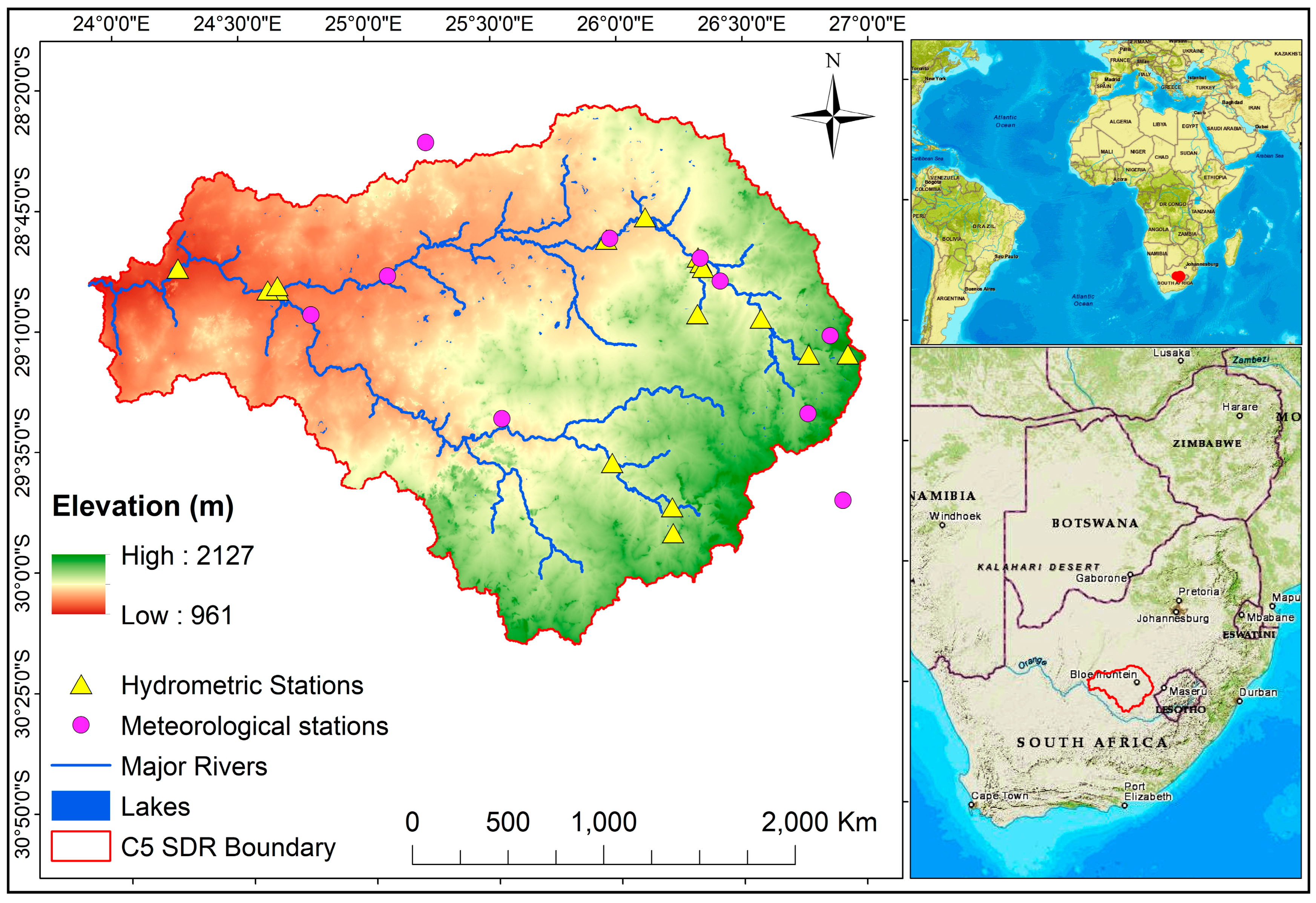
The C5 SDR, the research area, is roughly 35,570 km² in size and is a portion of primary drainage region C (Figure 1). Geographically, the study area spans roughly between 28–30° S latitude and 24–27° E longitude (Figure 1). At a spatial resolution of 30 m, it was delineated using a Digital Elevation Model (DEM) dataset. USGS EarthExplorer is where the dataset was obtained [34]. In terms of hydrology, South Africa is divided into 22 primary drainage regions and 148 secondary drainage regions [26]. The Riet (C51) and Modder (C52) River systems in central South Africa are part of the C5 SDR. Each of the 23 quaternary catchments that make up these basins empties into the Orange-Vaal River system [35]. Additionally, an ecotone that divides the grassland and eastern Nama Karoo biomes is where the C5 SDR is located [12,36]. The western and central parts are situated in the semi-arid Eastern Nama Karoo (300–500 mm/year) [37], and have shallow stony soils with vegetation dominated by drought-tolerant grasses (Themeda triandra, Eragrostis spp.) and dwarf shrubs (Pentzia incana, Eriocephalus spp.). The eastern section is in the Grassland biome (>500 mm/year), which sustains continuous grass cover dominated by T. triandra, Tristachya leucothrix, and E. curvula [12]. Woody species are restricted to drainage lines. This transitional habitat is particularly susceptible to climate and land use changes, which can affect ecosystem services and change the vegetation balance [38].

The climate of the C5 watershed is primarily semi-arid and exhibits significant seasonal and geographical variability. Mean annual precipitation (MAP) varies from approximately 275 mm in the western low-lying areas to over 686 mm in the eastern uplands, with the basin-wide average being close to 424 mm [26,28]. Rainfall is highly seasonal in the C5 SDR. While the watershed winters (May to August) are usually dry, it generally happens during the austral summer months (September to April), reaching its highest intensities in January and February [26]. The highest average monthly temperature in the basin is between 18.1 °C in the winter and 31.2 °C in the summer. In winter, the minimum average monthly temperature is −1.3 °C, while in summer, it is 15.4 °C. The region’s topography is gently undulating, with elevations ranging from 2127 m east to 961 m west above mean sea level and slopes varying from 1.7% to 10.3% (Figure 1). A network including 223 South African Weather Service (SAWS) daily rainfall stations, 185 of which are situated inside the C5 region and 38 outside, provides adequate spatial coverage for climatic research [26]. Figure 1 only shows a small subset of the operational stations that were obtained from SAWS upon request. As shown in Figure 1, the basin contains 16 active hydrometric stations, which, together with the weather stations provide spatial context for hydrological and climatic monitoring within the catchment.

Socioeconomically, the area is predominantly rural, with low population density and livelihoods primarily dependent on rainfed and irrigated agriculture, livestock rearing, and related land-based activities. Bloemfontein and Kimberley serve as the principal urban and economic centers, providing markets, services, and infrastructure that influence land use patterns and resource utilization across the surrounding rural landscape [39].

2.2. Sources of Data

The SANLC datasets, which offer open-access, satellite-derived land cover data throughout South Africa, including the C5 SDR, serve as the study’s main data source.

The 1990 land-cover dataset was derived from Landsat 4 and 5 Thematic Mapper (TM) imagery with a spatial resolution of 30 m, acquired between April 1989 and October 1991 [40]. For 2014, 30 m Landsat 8 Operational Land Imager (OLI) scenes captured between April 2013 and March 2014 were utilized [41]. The 2022 dataset was developed using Sentinel-2 multispectral imagery (20 m resolution) collected throughout the year, from January to December 2022 [42]. Each dataset incorporated multi-temporal acquisitions covering different seasons to represent vegetation phenology and land-cover variability effectively. Only cloud-free scenes were included to maintain temporal consistency; however, minor cloud-affected areas were rectified by compositing with adjacent cloud-free images to reduce spectral distortion. All Landsat data (4, 5, and 8) were obtained from the U.S. Geological Survey (USGS) online archive (https://glovis.usgs.gov/).

The datasets used in this study were provided by the Department of Forestry, Fisheries, and the Environment (DFFE) through the Environmental Geographic Information Systems (EGIS) platform upon request on 05 June 2025 [33]. Developed in accordance with the national land cover classification standard (SANS 19144-2), these datasets are available for 1990, 2014, 2018, and 2022, and can be accessed at (https://www.dffe.gov.za/egis, accessed on 5 June 2025).

2.3. Accuracy Validation and Workflow for Land Use Classification

The SANLC datasets for 1990, 2014, and 2022 were created using automated mapping model, reproducible classification workflows applied to satellite imagery [24]. Recent iterations, such as SANLC 2018 and later, rely mainly on 20 m multi-seasonal Sentinel-2 data, complemented by historical Landsat TM, ETM+, and OLI imagery to ensure consistency over time. All datasets follow the nationally mandated land cover standard (SANS 19144-2), which defined detailed classes aligned for temporal comparability [33].

Several important steps were involved in the classification process. As part of the initial preprocessing, Sentinel and Landsat scenes were mosaicked and atmospheric correction were applied. The core land-cover classification was performed using automated mapping approaches that combined rule-based spectral modeling with machine learning algorithms, ensuring accurate delineation of spatial and temporal variability in land cover. Initially included 72 land cover classes for 1990 and 2014 and 73 for 2022. To facilitate interpretation, modelling, and analysis, the records were methodically combined into nine more comprehensive hierarchical LULC categories as recommended [35]. To improve analytical clarity and modelling efficiency, the categories include waterbodies (WB), forested lands (FL), grassland (GL), wetlands (WL), cultivated land (C), shrubland (SH), built-up areas (B), bare land (BL), and mines/quarries (MQ). Detailed descriptions of these classes are provided in

Table 1. Description of land use and land cover (LULC) classes identified in the study area.

LULC Classe	Description
Bareland (BL)	Natural rock surfaces, dry pans, eroded lands, bare riverbed materials and others
Built-up area (B)	Residential, Villages, Smallholding, Urban vegetation, commercial, industrial and transport
Cultivated land (C)	Permanent crops, Temporary Crops, Fallow Lands and old Fields
Forested Lands (FL)	Contiguous low forest and thicket, dense forest and wooded, open woodland, contiguous and dense plantation forest, open and sparse plantation forest, clear-felled plantation forest
Grassland	Sparsely wooded grassland, and natural grassland
Mines/quarries (MQ)	Surface infrastructure, extraction pits, quarries, salt mines, tailings and resource dumps and landfills
Shrubland (SH)	Low shrubland and Nama Karoo
Waterbodies (WB)	Natural Rivers, natural pans, artificial dams (including canals), artificial sewage ponds, artificial flooded mine pits
Wetlands (WL)	Herbaceous wetlands

. This thematic simplification preserves classification uniformity and spatial relevance, aligning with the SANLC grouping structure [35,36,37].

Strict procedures overseen by the DFFE platform were followed during validation and accuracy evaluation [33]. Reference datasets were produced using ground truth data, reliable shapefiles, and the interpretation of high-resolution images. To compute important accuracy metrics, such as Overall Accuracy (OA), User’s Accuracy (UA), Producer’s Accuracy (PA), and the Kappa Coefficient (κ), confusion matrices were built. All associated metadata including the full accuracy assessment (per-class accuracy matrix), dataset version, classification legends, and detailed land-cover map reports describing the LULC classes listed in Table 1 are available from the DFFE Geoportal (https://www.dffe.gov.za/egis, accessed on 5 June 2025), accessed on 5 June 2025. The SANLC-derived land cover maps used in this investigation are both methodologically sound and extensively confirmed thanks to these coupled methodological methods, which also serve as a solid basis for subsequent spatiotemporal land cover change analysis [33,42].

The land-cover datasets were generated from different satellite sensors, including 30 m Landsat imagery for 1990 and 2014, and 20 m Sentinel-2 imagery for 2022. To ensure spatial compatibility with the earlier Landsat datasets, the 2022 Sentinel-2 data were resampled to 30 m using the nearest-neighbor method prior to performing change detection. Furthermore, to maintain consistency and enable direct comparison across all datasets, the classification legends were harmonized and standardized, as detailed in Table 1.

2.4. Methods of Detecting Changes in Land Use and Land Cover

Following the harmonization of the LULC maps and their classification legends, a post-classification change detection approach was employed to analyze land-use and land-cover dynamics. This was implemented in the TerrSet liberaGIS v20.03 environment, which overlays independently classified LULC maps from multiple years to detect and quantify pixel-level transitions among land-cover classes. The analysis was conducted over three periods: 1990–2014, 2014–2022, and 1990–2022. Using the Land Change Modeller (LCM) in TerrSet liberaGIS v20.03, a comprehensive set of change metrics was generated, including gross gain (the total area a land-cover class gained from other classes), gross loss (the total area a class lost to others), and net change (the difference between gains and losses). Percentage net change provided information on the proportion of total area affected within each class, while the rate of change was calculated to assess the temporal velocity of LULC transformations.

$$P_c=\left({\displaystyle \frac{A_f-A_i}{A_i}}\right)\times 100$$

(1)

where $P_c$ is percent net change. $A_i$ is the area of a class in the base year LULC map and $A_f$ is an area of a class in the later-year LULC map.

$$R_c={\displaystyle \frac{A_f-A_i}{t}}$$

(2)

where R_c is the annual rate of change in km², t is the time interval between base and final study years.

$$p_{ac}=\left({\displaystyle \frac{C_a}{T_a}}\right)\times 100$$

(3)

where $p_{ac}$ is the percentage area of a class, $T_a$ is total area and $C_a$ is an area of a class.

In addition, the directional dynamics of land cover transitions were quantified using an asymmetric change approach. It is a sophisticated approach that considers both land cover type increases and losses independently to give a more thorough grasp of patterns of landscape change. In the base year, each class’s percentage of loss was determined in relation to its area, and in the final year, the percentage of gain was determined in relation to its area. A directional perspective on land cover transformation and the changing dominance or decline of classes was provided by this asymmetric approach (Equations (4) and (5)). It supports more complex interpretations of landscape change for planning and policymaking by effectively capturing the non-reciprocal nature of class transitions.

$$p_l=\left({\displaystyle \frac{C_{al}}{A_i}}\right)\times 100$$

(4)

$$p_g=\left({\displaystyle \frac{C_{ag}}{A_f}}\right)\times 100$$

(5)

where $p_l$ represents the percentage of area lost for a given land cover class, $C_{al}$ is the total area lost from that class, and $A_i$ denotes the total area of the land cover class in the base year. Similarly, $p_g$ is the percentage of area gained for the class, $C_{ag}$ is the total area gained by the class, and $A_f$ is the total area of the study region in the later year.

Class-level contributor analysis was used to pinpoint the precise land cover categories influencing the growth or decline of a target class to facilitate a better comprehension of the underlying mechanisms. When a particular land cover class, for instance, showed a notable increase, the analysis identified the contributing classes from which this gain came; when a class was declining, the analysis identified the recipient classes to which its area was transferred. This clarified not only the extent of the changes but also their causes and effects. Furthermore, spatial patterns of stability and transformation throughout the landscape were visualized and interpreted using transition matrices, spatial trend maps, and change persistence analysis. A scientifically sound evaluation of the extent, direction, pace, and contributors of LULC change in the research area was made possible by the combined use of this integrated change detection system in TerrSet liberaGIS v20.03.

2.5. Methodology for Landscape Diversity Indices

Landscape diversity in the C5 catchment was assessed using Shannon’s Diversity Index (SHDI), Shannon’s Evenness Index (SHEI), and Simpson’s Diversity Index (SIDI) using QGIS v3.44.5 using the LecoS plugin v3.0.1. These indices quantify landscape heterogeneity, evenness, and dominance of land-cover classes [43].

$$SHDI=-{\sum }_{i=1}^m{P}_i\ln \left({\mathrm{p}}_i\right)$$

(6)

$$SHEI={\displaystyle \frac{SHDI}{\mathrm{l}\mathrm{n}\left(m\right)}}$$

(7)

$$SIDI=1-{\sum }_{i=1}^m{\mathrm{p}}_i^2$$

(8)

where

• m = number of land-cover classes
• $P_i$ = proportion of the landscape occupied by class i

All indices are unitless, with higher values indicating greater diversity or evenness. Calculations were performed in QGIS v3.44.5 using the LecoS plugin v3.0.1.

2.6. Patch Metrics

Patch metrics were calculated to quantify landscape structure and fragmentation within the C5 catchment using QGIS v3.44.5 with the LecoS plugin v3.0.1. The following metrics were used:

• Number of Patches (NP)

Total count of discrete patches of a given land-cover class. It counts (unitless). Higher NP indicates a more fragmented landscape.

2.

Patch Density (PD)

Patch density (PD) was calculated as the number of patches per 100 ha by dividing the number of patches by the total landscape area and multiplying by 10,000 to convert square meters to hectares. Higher PD indicates greater fragmentation; lower PD indicates more aggregation [14].

$$\mathrm{P}\mathrm{D}=\left({\displaystyle \raisebox{1ex}{$NP$}\!\left/ \!\raisebox{-1ex}{$A$}\right.}\right)\mathrm{10,000}$$

(9)

where NP = Number of patches; A = Total landscape area (ha).

3.

Mean Patch Area (MPA)

Mean Patch Area (MPA) represents the average size of patches within a given land-cover class and was used to evaluate landscape aggregation and fragmentation. It was calculated as the sum of the areas of all patches divided by the total number of patches:

$$\mathrm{MPA}={\displaystyle \frac{\sum a_i}{NP}}$$

(10)

where $a_i$ is the area of patch i (in hectares) and $NP$ is the number of patches. MPA is expressed in hectares (ha). Higher MPA values indicate larger, more contiguous patches and lower levels of fragmentation, whereas lower MPA values reflect smaller patch sizes and increased landscape fragmentation.

4.

Largest Patch Index (LPI)

Largest Patch Index (LPI) quantifies the dominance of the largest patch of a given land-cover class relative to the total landscape area [14]. It was calculated as:

$$\mathrm{LPI}=\left({\displaystyle \frac{a_{\mathrm{m}\mathrm{a}\mathrm{x}}}{A}}\right)\times 100$$

(11)

where $a_{\mathrm{m}\mathrm{a}\mathrm{x}}$ is the area of the largest patch (in hectares) and $A$ is the total landscape area (in hectares). LPI is expressed as a percentage (%). Higher LPI values indicate that a single patch dominates the landscape, reflecting greater spatial aggregation, whereas lower LPI values indicate a more fragmented landscape with no dominant patch. All metrics were calculated using projected CRS layers in QGIS v3.44.5, LecoS v3.0.1, ensuring areas were correctly measured in hectares.

3. Results

3.1. Spatiotemporal Patterns and Conversion Pathways of Land Cover

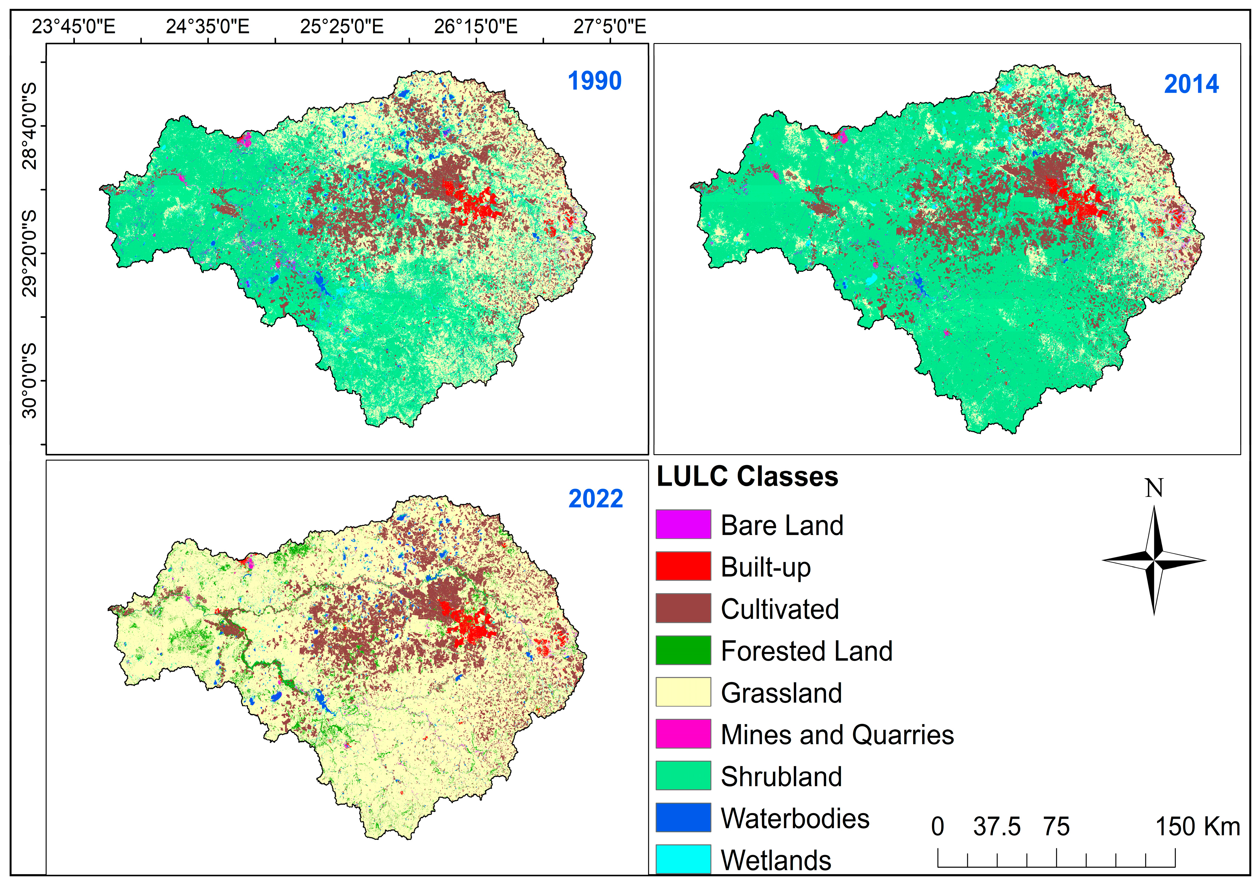
Between 1990 and 2022, the C5 SDR experienced notable transformations in land cover, reflecting the combined influence of anthropogenic activities and natural processes. As shown in Figure 2, the LULC maps for 1990, 2014, and 2022 reveal pronounced spatial and temporal variations across the landscape, encompassing nine dominant land-cover classes: BL, B, C, FL, GL, MQ, SH, WB, and WL.

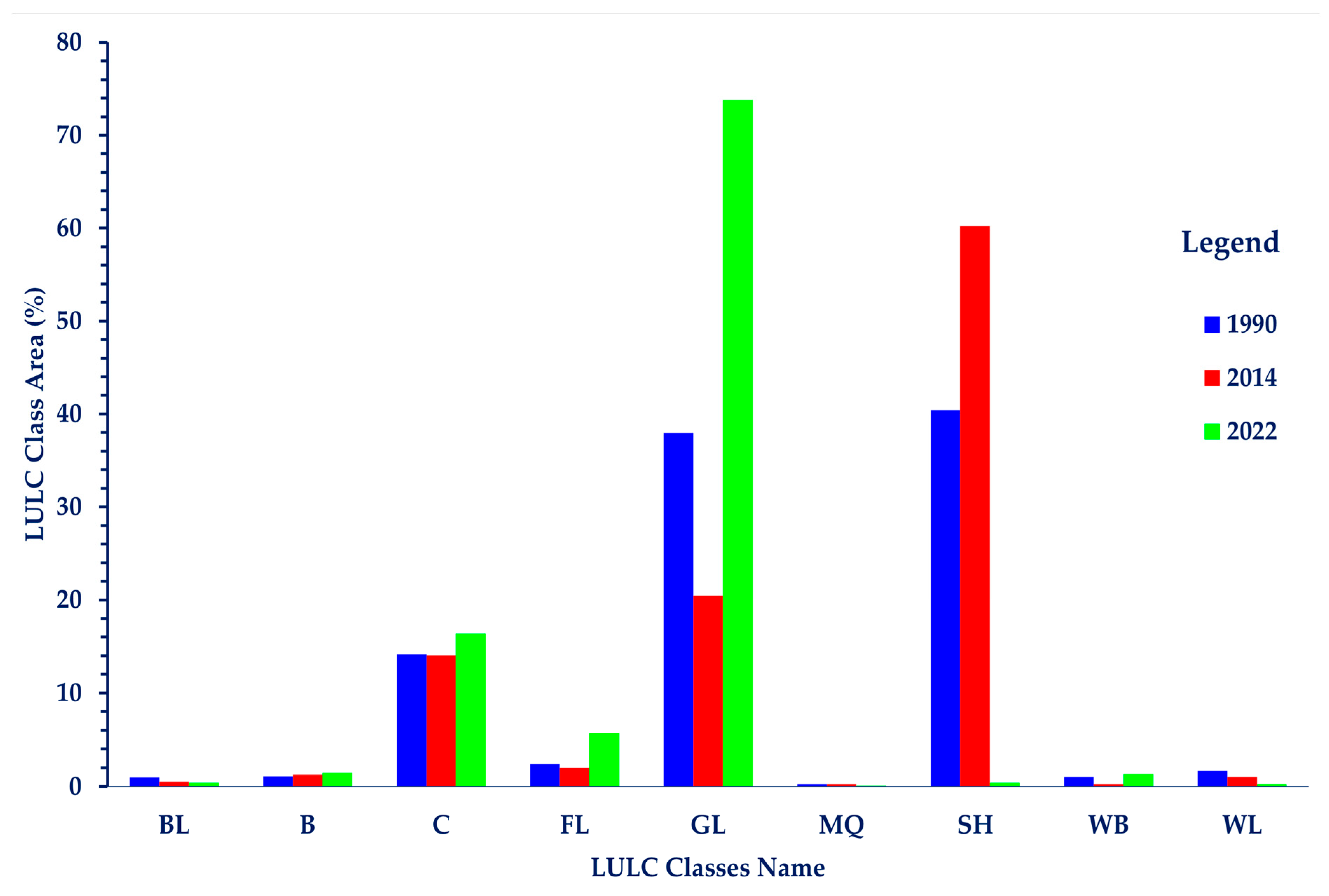
In 1990, the catchment landscape was primarily dominated by SH (40.4%), GL (38%), and C (14.2%), FL (2.4%), with WL (1.7%) and B (1.12%) occupying relatively smaller proportions (Figure 3). The SH covered extensive portions of the western, western central, and southern areas, while C appeared more scattered but was relatively concentrated in the northern, northeastern, northcentral, eastern and central zones (Figure 2). FL and WL were spatially fragmented, appearing mostly as isolated patches rather than continuous ecosystems.

By 2014, the landscape composition had shifted markedly. SH expanded to occupy 60% of the catchment, while GL and C decreased to 20% and 14%, respectively. B (1.3%) and WL (1%) persisted as minor components of the land cover mosaic (Figure 3), suggesting ongoing vegetation transitions and intensified human land use in localized zones.

In 2022, a pronounced shift in the landscape composition was observed. GL became the dominant land cover type, occupying 74% of the catchment, followed by C (16.41%) and FL (5.73%). B and WB also showed slight increases, covering 1.5% and 1.33% of the total area, respectively (Figure 3). A notable expansion of WB was recorded from 375 km² in 1990 to 471.3 km² in 2022 (

Table 2. Land Use and Land Cover (LULC) transition matrices for 1990–2014, 2014–2022, and 1990–2022 showing class totals, annual rate of change, gains, losses, and persistence in km².

	1990	Classes	BL	B	C	FL	GL	MQ	SH	WB	WL	Total	Gain	Rate/Year
2014		BL	64	0.6	0.98	4	18.59	0.4	78.88	7.63	4.63	180.1	115.8	−7
		B	2.2	370	3.81	14	44.2	0.2	13.13	0.15	0.78	449	78.69	2.1
		C	2.1	1.7	4361	56	306.9	0.1	245.2	0.56	14.9	4989	627.3	−1.9
		FL	10	10	29.1	260	208.2	5	122.5	16.2	50.9	712.2	452.4	−5.7
		GL	21	8.3	234	278	4953	7.2	1579	33.9	154	7268	2315	−260
		MQ	0.1	0.2	0.99	4	6.857	79	1.187	0.12	1.03	93.11	14.45	−0.2
		SH	237	7.2	401	221	7947	6	12,319	51.3	230	21,420	9101	294
		WB	5.2	0	0.16	1.6	2.992	0	0.965	74.2	1.55	86.73	12.57	−12
		WL	4.8	0.5	1.98	10	15.01	0.5	9.257	191	138	371.4	233.6	−9.3
		Total	346	399	5033	849	13,503	98	14,370	375	596	35,570
		%	1	1.12	14.2	2.4	38	0.3	40.4	1.1	1.7	100
		Loss	282	29	672	590	8550	19	2051	301	458
	2014
2022		BL	17	1	0.46	5.6	15.21	0.3	77.63	0.29	28.9	145.9	129.4	−4.28
		B	4.5	411	12.6	18	30.11	0.8	43.31	0.04	0.68	521.4	110.5	8.94
		C	2.2	15	4665	43	376.2	0.5	732.3	0.25	2.75	5838	1173	106.2
		FL	7.4	8.4	45.5	285	609.4	4.2	1068	1.68	7.89	2037	1752	165.6
		GL	108	13	256	309	6154	37	19,314	1.88	60.3	26,252	20,099	2373
		MQ	1.4	0.5	0.52	2.6	1.577	33	3.072	0.02	0.73	43.02	10.48	−6.26
		SH	29	0.1	1.64	2.5	8.206	4.3	83.24	0.25	27.8	157.2	73.95	−2658
		WB	11	0.4	5.62	39	55.53	13	72.28	81.9	194	471.3	389.4	48.08
		WL	0.8	0.2	1.16	7.1	18.64	0.3	26.64	0.42	48.7	104	55.34	−33.4
		Total	180	450	4989	712	7268	93	21,420	86.7	371	35,570
		%	0.5	1.3	14	2	20.43	0.3	60.22	0.24	1.04	100
		Loss	164	39	323	427	1115	61	21,337	4.83	323
	1990
2022		BL	30	0.1	0.3	6.5	19.87	0.3	53.91	11.8	22.7	145.1	115.5	−6.29
		B	4.2	357	14.4	25	80.06	0.9	36.41	0.19	3.49	521.4	164.3	3.816
		C	4.4	15	4820	58	503.4	0.2	422	0.42	14.2	5838	1018	25.15
		FL	22	10	31.1	318	840.1	4.9	708.8	5.01	96.6	2037	1719	37.11
		GL	239	15	160	399	11,979	43	13,032	46.2	338	26,252	14,274	398.4
		MQ	1.1	0.4	0.77	2.9	3.65	31	2.582	0.15	0.59	43.02	12.05	−1.72
		SH	30	0.2	0.95	2.2	10.81	4.9	75.58	15.5	16.9	157.2	81.61	−444
		WB	14	0.3	4.25	27	40.85	12	24.11	289	59.4	471.3	181.9	3.003
		WL	2	0.5	0.96	11	25.19	0.4	13.82	6.56	43.9	104	60.14	−15.4
		Total	346	399	5033	849	13,503	98	14,370	375	596	35,570
		%	1	1.1	14.2	2.4	37.96	0.3	40.4	1.05	1.67	100
		Loss	317	42	213	531	1524	67	14,294	85.8	552

Note: Diagonal values are persistent and are highlighted in bold and color to facilitate clearer interpretation.

), indicating significant hydrological and geomorphological changes, possibly linked to dam construction, artificial impoundments, or increased surface runoff due to land disturbance.

Overall, these temporal patterns reveal a reorganization of the catchment’s ecological structure, characterized by the contraction of SH and the widespread conversion of former SH, BL and WL areas into GL. The observed transitions highlight the dynamic interplay between land management practices, vegetation succession, and hydrological alterations that have shaped the C5 SDR landscape over the past three decades.

3.1.1. LULCC Dynamics Between 1990 and 2014

Between 1990 and 2014, the C5 SDR experienced pronounced land cover transformations driven by a combination of anthropogenic activities and ecological processes. GL and WL showed major declines due to woody encroachment, agricultural expansion, drainage, and hydrological alterations. BL was primarily converted into FL, SH, and GL, suggesting natural vegetation succession and restoration processes (

Table 3. Transition Impact Matrix Showing Net Contributions of Land Cover Classes (Row) to the Net Change in all Other Classes (Column) in km² in the three study periods.

		Contributors to Net Change in
	Classes	BL	B	C	FL	GL	MQ	SH	WB	WL
	BL	0	2	2.1	10.1	20.51	0.1	237	5.2	4.78
	B	−2.18	0	−2.1	−3.9	−35.9	−0	−5.92	−0.1	−0.3
	C	−2.1	2	0	−27	−73.1	0.9	156.2	−0.4	−13
	FL	−10.1	4	27	0	70.22	−1	98.53	−15	−41
1990–2014	GL	−20.5	36	73	−70	0	−0	6367	−31	−139
	MQ	−0.09	0	−0.9	0.98	0.32	0	4.79	−0.1	−0.5
	SH	−237	6	−156	−99	−6367	−5	0	−50	−221
	WB	−5.23	0	0.4	14.6	30.94	0.1	50.34	0	190
	WL	−4.78	0	13	40.5	138.8	0.5	221	−190	0
	BL	0	3.5	1.7	1.8	92.6	1.1	−48.6	10	−28
	B	−3.5	0	2.5	−10	−16.9	−0	−43.16	0.4	−0.5
	C	−1.7	−2	0	2.01	−121	0	−730.7	5.4	−1.6
	FL	−1.8	10	−2	0	−301	−2	−1065	37	−0.8
2014–2022	GL	−92.6	17	121	301	0	−36	−19,306	54	−42
	MQ	−1.1	0	−0	1.53	35.87	0	1.26	13	−0.4
	SH	48.6	43	731	1065	19,306	−1	0	72	−1.2
	WB	−10.2	−0	−5.4	−37	−53.7	−13	−72.03	0	−193
	WL	28	0	1.6	0.79	41.63	0.4	1.21	193	0
	BL	0	3	3.9	13.7	189.1	0.2	−36.65	0.2	−20
	B	−3.25	0	1.1	−14	−63.9	−1	−34.56	0.2	−2.9
	C	−3.91	−1	0	−27	−343	0.5	−420.2	3.8	−13
	FL	−13.7	14	27	0	−441	−2	−704.7	22	−86
1990–2022	GL	−189	64	343	441	0	−39	−12,964	−5.3	−311
	MQ	−0.17	1	−0.5	2.06	39.45	0	2.82	12	−0.2
	SH	36.7	35	420	705	12,964	−3	0	8	−2.6
	WB	−0.22	−0	−3.8	−22	5.34	−12	−8.03	0	−52
	WL	20.4	3	13	85.7	310.5	0.2	2.62	52	0

Note: Diagonal values (or zeros) represent contributors of a class to itself and are highlighted in color for clarity.

). In contrast, FL was mainly transformed into SH, GL C, and B, indicating anthropogenic encroachment, agricultural expansion, and landscape fragmentation (Table 3). The SH exhibited substantial expansion, primarily replacing GL and degraded areas, suggesting fire suppression, overgrazing, and climate-mediated vegetation shifts. B steadily increased due to urbanization and infrastructure development, whereas MQ showed minor net changes, reflecting operational shifts and natural revegetation. The marked decline in WB was likely associated with hydrological stress, sedimentation processes, and intensified water abstraction. Overall, the observed LULC dynamics indicate a strong directional trend toward SH dominated and anthropogenically influenced landscapes, with limited recovery in natural vegetation and water-dependent ecosystems.

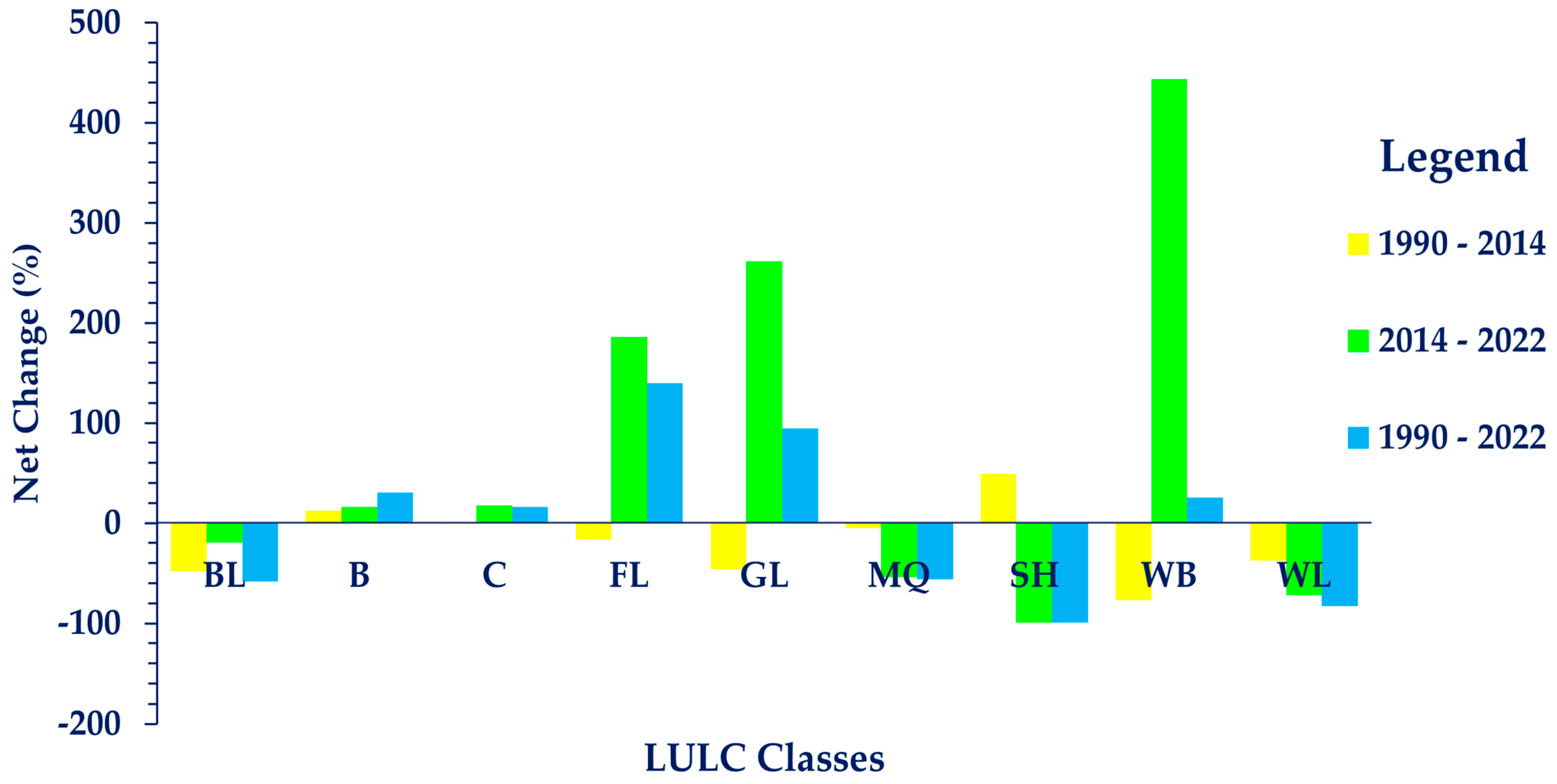
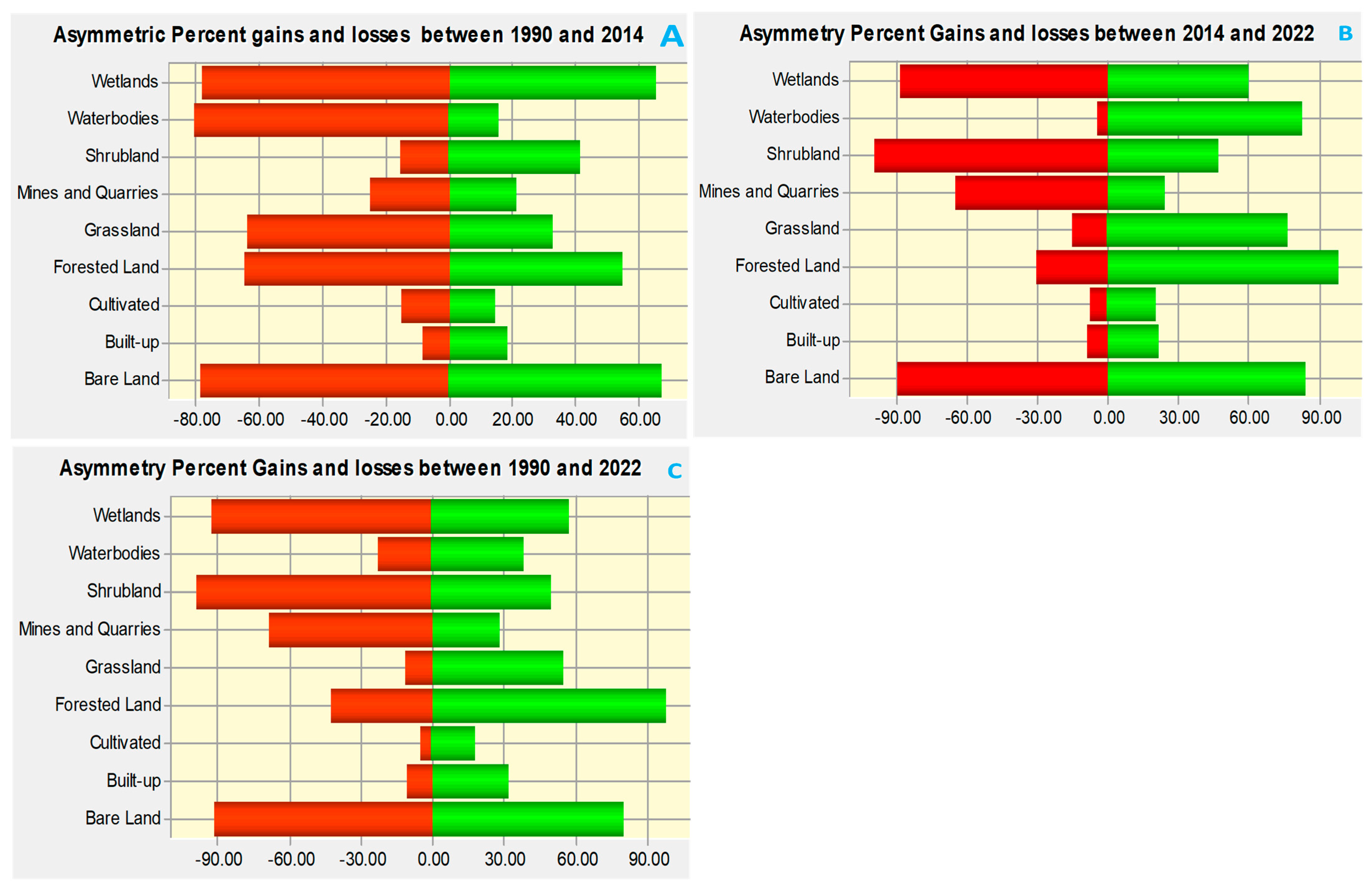
The BL contracted substantially from 346.2 km² to 180.1 km² which is a net loss of −166 km² (−48%), at a mean annual rate of −6.9 km² year⁻¹ (Table 2 and Figure 4). The decrease reflects colonization of exposed surfaces by vegetation, particularly SH, as well as conversion into FL. The total gains from other classes (116 km²) likely correspond to localized soil exposure caused by erosion, overgrazing, or temporary land clearing. The pronounced asymmetry, with 81.4% of BL loss contrasted by 64.3% of BL gain (Figure 5), indicates a partial net recovery of previously bare or sparsely vegetated areas toward more vegetated or developed land cover types. Major net losses occurred primarily to SH (−237 km²), GL (−20.5 km²), FL (10.1 km²) and B (−2.3 km²) (Table 3). Thus, the major negative contributors to the net change in BL were SH, GL, FL, and B, with no net positive contributors observed (Table 3).

In this study period, B increased moderately from 399 km² to 449 km² with net increase of +12.5% at 2.1 km² year⁻¹ (Table 2). This expansion is driven by infrastructure development, settlement growth, and peri-urban sprawl. Persistent B indicates limited land abandonment, while gains from GL, FL, and C reflect urban encroachment into previously natural or semi-natural landscapes. While the major positive contributors to the net change experienced by B were GL, FL, SH and C, there were not any negative contributors to the net change by B (Table 3). Low negative loss emphasizes the largely irreversible nature of urban expansion.

During this period, C remained relatively stable. It decreased slightly from 5033 km² to 4989 km² with net loss of −0.9% at annual rate of change of −1.9 km² year⁻¹ (Table 2 and Figure 4). The persistence of C was 4361 km². Losses to SH indicate land abandonment or conversion of marginal fields due to reduced productivity, soil degradation, or climatic stress. Gains from GL, SH, FL, and WL reflect agricultural intensification and expansion into ecotonal areas driven by population growth. The net expansion of C was primarily driven by gains from GL (73 km²), FL (27 km²), and WL (13 km²) whereas the net contraction of C was chiefly associated with losses in SH (−156 km²) and B (−2 km²), highlighting asymmetric contributions of different land cover classes to the overall landscape change (Table 3).

FL declined from 849.5 km² to 712 km² with net decrease of −16%) at −5.7 km² year⁻¹ (Table 2 and Figure 4). The reduction was primarily attributed to deforestation associated with the expansion of C and B, fuelwood harvesting, and subsequent degradation into GL and SH. Gains from WL indicate localized reforestation or natural succession in previously waterlogged areas. The observed asymmetry, with 69.4% loss versus 63.5% gain (Figure 5), indicates that FL recovery was insufficient to compensate for net deforestation, highlighting a persistent decline in forested areas.

GL experienced the largest decline, from 13,502 km² to 7268.4 km² which is about −46% net loss at −260 km² year⁻¹ (Table 2 and Figure 4). The major negative contributors to this change were SH (−6367 km²), C (−73 km²), and B (−35.9 km²), while major positive contributions came from WL (139 km²), FL (70 km²) and WB (31 km²), (Table 3), highlighting the pronounced asymmetry in landscape transformation. Asymmetric analysis with −63.3% loss versus 31.9% gain, indicated that losses of GL to other LULC classes far exceeded gains from them (Figure 5), highlighting a pronounced imbalance in landscape transformation. The net decline was primarily driven by conversion to SH likely due to woody encroachment, fire suppression, overgrazing, and climate-induced vegetation shifts. Additional losses to C and B reflect agricultural expansion, cropland intensification, urbanization, and infrastructure development. Gains from WL, WB, and FL indicate localized vegetation regrowth or possible reclassification, though these increases were insufficient to offset the dominant losses. As depicted in Figure S1A, grassland was extensively lost, particularly in the central, south-central, and southeastern zones.

MQ decreased slightly from 98 km² to 93 km² (−5%) at −0.2 km² year⁻¹ (Table 2 and Figure 4). The modest decline reflects operational shifts, reclamation, or natural revegetation of abandoned sites. GL contributed most to the loss, consistent with spontaneous colonization of disturbed areas.

SH expanded from 14,369.7 km² to 21,420.1 km² (+49%) at 294 km² year⁻¹ annual rate of change (Table 2 and Figure 4). This expansion is primarily due to GL conversion via woody encroachment driven by reduced fire frequency, overgrazing, and climate variability. Additional gains from WL, C, and BL reflect both ecological succession and land degradation. B (−5.9 km²) was the only significant negative contributor (Table 3). As shown in Figure S1C, shrubland expanded widely, replacing grassland and wetland, especially in the central, south-central, and eastern parts of the catchment. This indicates ecological degradation and vegetation densification.

WB declined sharply from 375 km² to 86.7 km² with a net loss of −77% at −12 km² year⁻¹ (Table 2 and Figure 4), largely due to hydrological stress, sedimentation, and water abstraction for C and settlements. The asymmetric statistics showing a −80.2% loss relative to 1990 and a 14.5% gain relative to 2014 indicate a marked net reduction in WB, reflecting substantial depletion with limited recovery, likely associated with fluctuations in surface water availability and hydrological stress (Figure 5). Losses to WL reflect conversion of shallow water zones into marshy or seasonally wet areas, while minor losses to GL and SH indicate progressive drying and vegetation encroachment.

WL decreased from 595.6 km² to 371.4 km² with a net decrease of −38% at −9.3 km² year⁻¹ (Table 2 and Figure 4). Contraction resulted from drainage for C, encroachment by SH and GL, and altered hydrological regimes due to upstream water abstraction and climate variability. Gains from WB likely reflect seasonal fluctuations. The asymmetric statistics, showing a −76.9% loss relative to 1990 and a 62.9% gain relative to 2014 (Figure 5), indicate a substantial net decline of WL, with major transitions to SH (−221 km²), GL (−139 km²), FL (−41) and C (−13 km²) (Table 3). The positive contributors to the net change experienced by WL were WB (190 km²) and BL (4.8%) (Table 3).

3.1.2. LULCC Dynamics Between 2014 and 2022

Between 2014 and 2022, the C5 SDR underwent extensive land cover transitions that reveal both rapid ecological reorganization and intensified human-induced landscape modification. The period was marked by strong contrasts, massive contraction of SH and WL, accompanied by unprecedented expansion of GL, FL, and WB (Table 2). These shifts reflect the combined influence of land management practices, climate variability, vegetation succession, and anthropogenic development pressures. The directionality of change suggests a broad transition from woody and semi-natural cover toward open grass-dominated systems, recovering forests in riparian zones, and increased aquatic features.

BL continued its long-term decline, decreasing from 180.1 km² in 2014 to 145.9 km² in 2022 with a net loss of 34.2 km² (−19%) at an annual rate of 4.3 km² year⁻¹ (Table 2 and Figure 4). Only 16.6 km² remained persistent, confirming that most previously exposed surfaces were converted. The major net losses occurred to GL (−92.6 km²), WB (−10.2 km²), FL (−1.8 km²), C (−1.7 km²), and B (−3.5 km²) (Table 3), indicating active vegetation recovery, afforestation, and agricultural or infrastructural encroachment. Conversely, BL recorded localized net gains (121.7 km²) from SH (+48.6 km²) and WL (+28 km²) (Table 3), reflecting soil exposure due to erosion, vegetation clearing, and temporary degradation. The strong asymmetry between gains (88.7%) and losses (−90.8%) emphasizes the dominance of ecological recovery processes over degradation during this period (Figure 5).

The B class exhibited a consistent expansion from 449.9 km² in 2014 to 521.4 km² in 2022, representing a net increase of +15.9% at a rate of 8.9 km² year⁻¹ (Table 2 and Figure 4). A substantial portion, about 410.9 km², remained unchanged, indicating very high spatial persistence of existing infrastructure (Table 2). The net gain of 71.5 km² was mainly driven by urban growth and rural-to-urban transformation, supported by net inflows from SH (+43 km²), GL (+17 km²), FL (10 km²) and BL (+3.5 km²) (Table 3). These transitions emphasize ongoing peri-urban expansion and infill development consistent with population increase and intensified economic activity. Minor net outflows to C (−2 km²) are likely due to land abandonment. The asymmetric statistics −9% loss relative to 2014 and 21.2% gain relative to 2022 indicates a strong expansion tendency, with gains far exceeding losses and persistence remaining markedly high.

The C land expanded significantly, increasing from 4988.5 km² in 2014 to 5838 km² in 2022 with a net gain of 849.6 km² (+17.1%) at 106.2 km² year⁻¹ (Table 2 and Figure 4). Persistent agricultural land covered 4665.3 km², indicating strong continuity of existing croplands (Table 2). The main net contributors to expansion were SH (+731 km²), GL (+121 km²), and BL (+1.7 km²) (Table 3), suggesting the transformation of semi-natural and degraded areas into agricultural fields. These changes align with regional agricultural intensification and increased demand for arable land. The net losses to FL (−2 km²) and WB (−5.4 km²) (Table 3), likely are due to localized flooding, abandonment, or land reallocation. The overall trend reflects a combination of intensified cultivation and dynamic land use redistribution driven by demographic and economic pressures.

FL showed the most pronounced proportional increase, expanding from 712.2 km² to 2037 km² with net gain of +186% at an exceptional rate of 165.6 km² year⁻¹ (Table 2 and Figure 4). Persistent FL accounted for only 284.9 km² (Table 2), with most net gains derived from SH (+1065 km²), GL (+301 km²), C (+2 km²), and BL (+1.8 km²) (Table 3). The sharp increase suggests large-scale natural succession and riparian forest regeneration along river corridors and drainage lines. This expansion likely reflects enhanced vegetation recovery following reduced anthropogenic disturbance, favorable moisture regimes, and potential reforestation or conservation efforts. The dominance of inflows over outflows demonstrates a strong ecological recovery trajectory during this interval.

GL underwent an extensive resurgence, expanding from 7268.4 km² to 26,252 km² with a net gain of +261.2%) at a rate of 2373 km² year⁻¹ (Table 2 and Figure 4). Of this, 6153.5 km² remained persistent, while gross gains reached 20,099 km². The dominant net positive contribution came from SH (+19,306 km (Table 3) indicating large-scale woody vegetation clearance or dieback. Additional net gains originated from BL (+92.6 km²), WL (+41.6 km²), and MQ (+36 km²) (Table 3). These transitions point to widespread landscape opening through degradation, fire activity, overgrazing, and climate-induced vegetation shifts. Meanwhile, GL experienced net losses to FL (−301 km²), C (−121 km²), WB (−53.7 km²) and B (−16.9 km²) (Table 3), represent localized afforestation and land intensification. The overwhelming net expansion marks GL as the dominant landscape type in 2022. The asymmetric statistics, indicating a 15% loss relative to the 2014 base year and a 76.6% gain relative to the 2022 end year, reveal a pronounced expansion dynamic for GL (Figure 5), where gains overwhelmingly surpassed losses, signifying substantial net growth and spatial reoccupation across the landscape.

MQ declined from 93 km² to 43 km² with net loss of −53.8% at −6.3 km² year⁻¹ (Table 2 and Figure 4). This reflects the reduction in mining intensity and post-extractive landscape recovery. Only 32.5 km² persisted, while 60.6 km² transitioned to other land classes (Table 2). The largest recipients were GL (−36 km²) and WB (−13 km²) (Table 3), consistent with vegetation colonization of abandoned mines and water accumulation in quarry pits. These transitions suggest spontaneous ecological rehabilitation or deliberate reclamation, leading to improved soil stability and local biodiversity. Limited new MQ formation (10.5 km²) indicates decreased extractive expansion, possibly due to resource depletion or regulatory constraints (Table 2).

SH experienced a near-total collapse, declining from 21,420 km² to 157.01 km², with the net loss of −99.3% at −2658 km² year⁻¹ (Table 2 and Figure 4). Only 83.2 km² persisted, while 21,366.8 km² converted to other classes. Major net losses were to GL (−19,306 km²), FL (−1065 km²), C (−730.7 km²), WB (−72 km²), B (−43.2 km²), and BL (−46.8 km²) (Table 3). This abrupt reduction indicates a systemic collapse of woody vegetation, likely driven by intensive clearance, fire disturbance, grazing pressure, and prolonged drought stress. Minimal gains (74 km²) from other classes failed to compensate for these losses. The asymmetric statistics, showing a −99.6% loss relative to the 2014 base year and a 47% gain relative to the 2022 end year, indicate a severe contraction of SH (Figure 5), with extensive losses far outweighing localized recoveries, reflecting a dominant and near-total decline in spatial extent. The transformation marks a fundamental ecological shift from shrub-dominated to grass-dominated systems.

The WB expanded dramatically from 86.7 km² to 471 km² with a net gain of +443.5% at 48.1 km² year⁻¹ (Table 2 and Figure 4), driven by hydrological processes and land-use legacy effects. The major positive contributors were WL (+193 km²), SH (+72 km²), and GL (+54 km²) (Table 3). The asymmetric statistics, with a −5.6% loss relative to the 2014 base year and an 82.6% gain relative to the 2022 end year, indicate a substantial expansion of WB, where moderate losses were greatly outweighed by significant gains, reflecting marked hydrological variability and surface water increase during the period. These transitions likely reflect increased surface water accumulation due to flooding of low-lying areas, reservoir development, and inundation of former quarry sites. The strong directional trend toward aquatic expansion suggests hydrological alteration, possibly linked to higher rainfall variability or anthropogenic impoundments.

The WL, conversely, contracted severely from 371.4 km² to 104 km² with a net loss of −72% at −33.4 km² year⁻¹ (Table 2 and Figure 4). Only 48.7 km² remained persistent, with net losses (−267.3 km²) largely transitioning to WB and GL (Table 3). This reduction indicates extensive drainage, siltation, and vegetation encroachment. The gains (55.3 km²) were insufficient to offset widespread wetland loss, underscoring continuing hydrological stress and ecosystem vulnerability. In contrast to WB, the asymmetric statistics for Wetland (WL), showing an −86.9% loss relative to the 2014 base year and a 53.2% gain relative to the 2022 end year (Figure 5), reflect a strong net contraction, where extensive losses dominated despite partial recovery, indicating continued wetland degradation and fragmentation across the catchment.

Overall, the 2014–2022 period was characterized by accelerated and asymmetric LULC transformations. The simultaneous collapse of SH and WL alongside the expansion of GL, FL, and WB reveals a landscape undergoing rapid restructuring under coupled human–environment pressures, where degradation, recovery, and climate variability interact to redefine ecosystem composition and spatial configuration.

3.1.3. Cumulative LULCC Dynamics Between 1990 and 2022

Between 1990 and 2022, the C5 SDR experienced profound and spatially heterogeneous land cover transformations, indicative of long-term anthropogenic expansion, ecological recovery, and climate-mediated reorganization. The cumulative 32-year transitions reveal a directional landscape trajectory dominated by the large-scale replacement of shrubland (SH) with grassland (GL), forestland (FL), and cultivated land (C), accompanied by hydrological and infrastructural adjustments. Overall, the pattern demonstrates a shift from woody and semi-arid shrub-dominated systems toward more open, herbaceous, and mixed-use mosaics, with pockets of reforestation and aquatic expansion.

Over the full 32-year period, BL exhibited a sustained and substantial contraction. It decreased from 346 km² in 1990 to 145 km² in 2022. This represents a net reduction of 201 km² (−58.1%) at an average annual rate of −6.3 km² year⁻¹ (Table 2 and Figure 4). Persistent BL covered only 29.5 km², while 317 km² was converted to vegetated or developed classes and 115.6 km² gained from other types (Table 2). The strong asymmetry −91.5% loss relative to the base year and 79.7% gain relative to the end year, indicates long-term stabilization under vegetation recovery rather than renewed exposure (Figure 5). The dominant conversions to GL (−189 km²) and FL (−13.7 km²) (Table 3). This suggests extensive revegetation through natural colonization or passive rehabilitation. Localized gains from SH (+36.7 km²) and WL (+20.4 km²) (Table 3), indicate small-scale degradation or hydrological disturbance, yet insufficient to reverse the broader decline.

The B land expanded consistently, rising from 399 km² to 521 km² with a net gain of +122 km² (+30.6%) at 3.8 km² year⁻¹ (Table 2 and Figure 4). Approximately 357 km² remained persistent in eastern central part (Figure S2), while 42.2 km² was lost and 164 km² gained from other covers (Table 2). The gain-dominant asymmetry (31.5% gain vs. 10.6% loss) demonstrates a unidirectional urban expansion typical of settlement growth (Figure 5). The net inflows came from GL (+64 km²) and SH (+35 km²), FL (+14 km²) reflecting peri-urban encroachment and densification along infrastructure corridors (Table 3). Limited losses to vegetated classes indicate reclassification or vegetation regrowth in low-density zones, but the overall trend denotes irreversible urbanization. Figure S1C shows that B exhibits moderate but continuous expansion in central-eastern and northeastern towns, mainly around infrastructure corridors. Growth remained small but consistent, reflecting steady urbanization.

The C land increased moderately yet persistently, from 5033 km² in 1990 to 5838 km² in 2022 which is a net increase of +804.6 km² (+16.0%) at 25.1 km² year⁻¹ (Table 2 and Figure 4). Persistence was high (4820 km²) in the central and northeastern part of the catchment (Figure S2), but 1017.8 km² was newly converted from other classes (Table 2). The positive contributors for the net change by C were SH (+420 km²), GL (+343 km²), FL (27 km²), WL (+13 km²) and BL (+3.9 km²) (Table 3). The net pattern indicates steady agricultural expansion into semi-natural rangelands, likely driven by demographic and economic pressures. Net losses to WB (−3.8 km²) were limited, suggesting inundation in flood-prone zones. The asymmetric ratio (17.4% gain vs. 4% loss) confirms the directional, expansionary trajectory of agriculture (Figure 5). Figure S1C illustrates the expansion of C, mostly in the northeastern, central and eastern zones. Cultivated land often expanded into shrubland and grassland.

The FL expanded dramatically, from 849 km² to 2037 km² with a net gain of +1188 km² (+140%) at 37.1 km² year⁻¹ (Table 2 and Figure 4), marking one of the most remarkable ecological recoveries. Only 318 km² persisted, while 531 km² was lost and 1718.9 km² gained (Table 2). Figure S2 shows pronounced FL expansion along riverbanks in the eastern and southwestern, driven by favorable riparian microclimates, hydrological stability, and low human disturbance, with a notable asymmetric transition. The positive contributors to the net change experienced by FL were SH (+705 km²) and GL (+441 km²) (Table 3). The strong asymmetry (84.4% of 2022 FL derived from gains) demonstrates widespread forest colonization and riparian regeneration along the Modder–Riet drainage network (Figure 5). These gains likely reflect reduced anthropogenic disturbance, natural succession, and possible afforestation or conservation programs. Limited net transitions from C, BL, and WL indicate localized reforestation of cultivated and degraded land (Table 3).

The GL showed exceptional and spatially extensive expansion, increasing from 13,503 km² to 26,252 km² (+12,750 km²; +94.4%) at 398 km² year⁻¹ (Table 2 and Figure 4). Persistence reached 11,979 km², while 1524 km² was lost and 14,273.8 km² gained (Table 2). Spatially, the gain concentrated in the western and southwestern locations (Figure S2). The major contributors to the net gain were SH (+12,964 km²), WL (310.5 km² and BL (189 km²) and MQ (39.5 km²) (Table 3). These increases were likely associated with large-scale vegetation opening and shrub reduction, driven by fire disturbances, overgrazing, drought, and management-induced changes. The asymmetric pattern (54.4% of 2022 GL from gains vs. 11.3% 1990 loss) highlights directional replacement of woody cover by herbaceous vegetation (Figure 5). Net losses to FL (−441 km²), C (−343 km²), and B (−64 km²) show concurrent land intensification in specific zones (Table 3). Significant net gains in grassland occurred, particularly in the western, western central, central and southwestern and southern sectors, where shrubland loss was concentrated within ecotonal zones (Figure S1C).

MQ declined markedly from 98 km² to 43 km² which is a net of −55 km² (−56.2%) at −1.7 km² year⁻¹ (Table 2 and Figure 4), consistent with mining reduction or post-extractive rehabilitation. Only 31 km² persisted; 67 km² was converted, and 12 km² gained anew (Table 2). The directional asymmetry, showing a 68% loss relative to the base year and a 28% gain relative to the end year, indicates progressive abandonment, where losses far outweighed gains, reflecting sustained decline (Figure 5). Major net transitions were toward GL (−39 km²), WB (−12 km²), SH (−3 km²), and FL (−2 km²) (Table 3), implying ecological succession and hydrological infill of inactive sites, especially in lower-elevation areas. New MQ formation was minimal, reflecting reduced extraction intensity.

The SH underwent near-total collapse, declining from 14,370 km² to 157 km² about a net decrease of −14,212 km² which is −98.9% at −444 km² year⁻¹ (Table 2 and Figure 4), the most extreme transition across all classes. Only 75.6 km² persisted, while 14,294 km² converted and 81.6 km² regenerated (Table 2). The asymmetric statistics, showing a 99.5% loss relative to the 1990 base year and a 51.9% gain relative to the 2022 end year, indicate a largely irreversible transformation of SH were extensive losses overwhelmingly surpassed limited recoveries, reflecting long-term landscape conversion (Figure 5). Most net losses occurred to GL (−12,964 km²), FL (−704.7 km²), and C (−420 km²), with smaller net shifts to B (−34.6 km²), BL (−36.7 km²), and WB (−8 km²) (Table 3). This pattern represents a major vegetation regime shift driven by prolonged drought, grazing, fire, and land clearing, reducing woody vegetation resilience and promoting grassland dominance across ecotonal landscapes.

Hydrological land covers displayed divergent trajectories. WB expanded from 375 km² to 471 km² with a net gain of +96 km² (+25.6%) at 3 km² year⁻¹ (Table 2 and Table 3). However, WL contracted sharply from 596 km² to 104 km² with a net decline of −491.6 km² (−82.5%) (Table 2 and Figure 4). The WB net expansion stemmed mainly from WL (+52 km²), FL (22 km²), SH (+8 km²), and MQ (+12 km²) (Table 3), reflecting surface water accumulation, damming, or quarry inundation. Figure S1C shows that a modest expansion in waterbodies, especially in the northeastern and central catchment, with wetland and shrubland converting to water. This suggests localized hydrological recovery or water impoundment development. The asymmetric statistics for WL, showing a −93% loss relative to the base year and a 57.8% gain relative to the end year, indicate a pronounced net decline, with losses overwhelmingly exceeding gains, reflecting substantial wetland degradation (Figure 4). For WB, the asymmetric statistics, showing a −22.9% loss relative to the base year and a 38.6% gain relative to the end year, indicate a moderate net increase, where gains slightly outweighed losses, reflecting partial recovery and expansion of surface water (Figure 5. Persistent WL declined markedly due to drainage, encroachment, and siltation, confirming long-term wetland degradation. Figure S1C depicts that the WL declined dramatically, especially in the central, northeastern, and eastern catchment, with dominant transitions to FL, WB, and GL. These contrasting hydrological dynamics highlight simultaneous wetland loss and open-water expansion, symptomatic of altered catchment hydrology and climate variability.

Cumulatively, 1990–2022 marks a transformative reconfiguration of the C5 SDR landscape. The dominance of GL, concurrent with the near-elimination of SH and strong FL recovery, signifies a biome-level transition from woody, semi-arid systems toward open, grass-dominated and mixed riparian landscapes. Agricultural and built-up expansions further reinforced anthropogenic imprint, while MQ contraction and WB expansion reflect both reduced extractive activity and altered hydrological regimes. Overall, these cumulative changes depict an ecosystem under dual trajectories of degradation and recovery where human pressure, vegetation succession, and climate variability interact to redefine the structural and functional integrity of the C5 catchment.

3.2. Spatial Trend of Change (STC) Analysis Across the Catchment

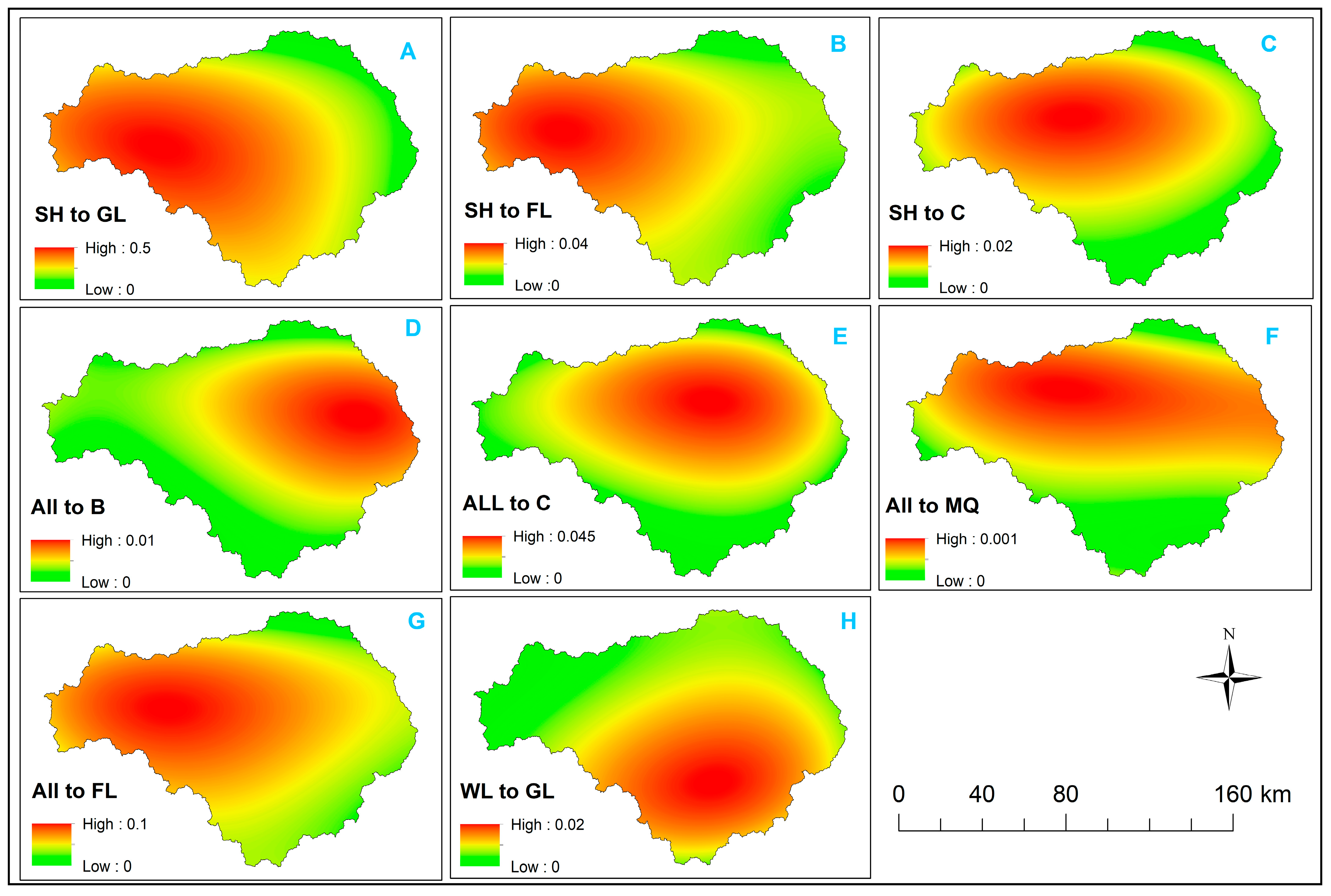
In the Land Change Modeler (LCM) of TerrSet liberaGIS v20.03, a binary change surface was generated by assigning a value of 1 to areas where other LULC classes were converted to a target class and 0 to areas with no change. These binary layers were treated as quantitative data to facilitate spatial trend analysis, modeling of change patterns, and statistical evaluation of drivers influencing land cover transitions. The major spatial trend of change (STC) provides a quantitative measure of the directional bias of conversion between land cover classes across the catchment. Higher STC values (approaching 1) indicate strong and spatially consistent transformation, while values near 0 reflect stability or negligible change.

As depicted in Figure 6, the STC analysis in TerrSet liberaGIS v20.03 revealed spatially asymmetric and class-specific land cover transitions across the C5 catchment. The conversion from SH to GL exhibited the highest STC (0.5) in western and southwestern sectors, indicating active shrubland-to-grassland conversion, while northern and northeastern zones showed no measurable change (STC = 0), reflecting persistent shrubland. The change from SH to FL (0.04) was restricted to western and central areas, with other zones showing no forest regeneration. The conversion from SH to C (0.02) occurred in central agricultural belts, whereas peripheral regions recorded no SH to C expansion. The transformation from all classes to C (0.05) indicated directional cropland growth in central and north-central sectors, while southern and western areas showed no expansion. The all classes to B transition (0.01) in the eastern sector denotes localized urban growth, whereas WL to GL (0.01) in the south reflects wetland degradation toward grassland. A minor all to MQ trend (0.001) extended along the northern corridor, indicating small-scale extraction or infrastructure development.

Overall, western and central sectors exhibit vegetation recovery, while central, eastern, and northern areas experience cropland expansion, degradation, or extraction. Zones of no change emphasize persistent landscapes, highlighting the interplay of biophysical stability and human-driven transformation, and providing spatially explicit guidance for land management and conservation.

3.3. Patch Metrics Trends

Patch metrics in the C5 catchment (

Table 4. Patch metrics (NP, PD, MPA, LPI) for each land-cover class in the C5 catchment for 1990, 2014, and 2022, showing temporal changes in landscape structure, fragmentation, and aggregation.

Years	Class Name	NP	PD (Patches/100 ha)	MPA (ha)	LPI (%)
	Bare Land	66,273	1.92	5082	0.007
	Built-up	592	1.71	656,328	0.51
	Cultivated	8416	2.43	581,438.8	1.5
1990	Forested Land	9032	2.6	7432.5	0.002
	Grassland	264,564	7.7	49,604	23.9
	Mines and Quarries	2337	6.8	40,869	0.05
	Shrubland	266,086	7.7	53,336	32.6
	Waterbodies	4807	1.4	75,819	0.1
	Wetlands	32,867	9.5	17,614.7	0.07
	Bare Land	36,836	1.1	6848.8	0.01
	Built-up	1151	3.3	379,520	0.33
	Cultivated	7664	2.3	608,916.6	1.5
	Forested Land	11,250	3.3	4677.8	0.002
2014	Grassland	207,214	6	34,099	9.3
	Mines and Quarries	2118	6	42,745.7	0.03
	Shrubland	140,112	4.1	152,801.7	55.4
	Waterbodies	2064	6	40,670	0.1
	Wetlands	12,027	3.5	30,025.7	0.07
	Bare Land	23,517	6.8	6007	0.003
	Built-up	20,381	5.9	24,752.7	0.7
	Cultivated	8123	2.4	698,629	2.1
	Forested Land	238,358	6.9	8306	0.27
2022	Grassland	69,813	2	655,518.6	72
	Mines and Quarries	2604	7.5	16,052.6	0.04
	Shrubland	46,610	1.4	3274	0.01
	Waterbodies	12,268	3.6	37,311.9	0.13
	Wetlands	13,379	3.9	7609	0.003

) show notable changes from 1990 to 2022. BL remained sparse and fragmented, with low LPI (<0.01) and moderate MPA (~5000–6000 ha), while PD increased slightly in 2022. Built-up and cultivated areas were highly aggregated, forming few large patches (MPA > 580,000 ha for cultivated land; LPI up to 0.7 for built-up). Forested land consisted of many small patches (NP = 238,358; MPA~8300 ha; LPI < 0.3), indicating persistent fragmentation. Grasslands coalesced, with declining NP and PD (69,813 and 2, respectively), large MPA (~655,000 ha), and high LPI (72), reflecting reduced fragmentation and increased dominance. Shrubland became highly fragmented, with low NP, PD, MPA, and LPI. Waterbodies and wetlands remained relatively stable, small, and low in dominance (LPI < 0.13). Overall, these trends indicate aggregation of human-modified landscapes, coalescence of grasslands, fragmentation of shrubland and forests, and stable but minor water-related patches, pointing to gradual landscape homogenization over the study period.

3.4. Landscape Diversity Indices

As

Table 5. Temporal dynamics of landscape diversity and evenness in the C5 catchment (1990–2022).

Year	Shannon Diversity Index (SHDI)	Shannon Equitability Index (SHEI)	Simpson Diversity Index (SIDI)
1990	1.3	0.6	0.7
2014	1.1	0.5	0.6
2022	0.9	0.4	0.43

illustrates, analysis of landscape diversity within the C5 catchment revealed a consistent decline across all three indices between 1990 and 2022. The Shannon’s Diversity Index (SHDI) decreased from 1.3 in 1990 to 0.9 in 2022, indicating a reduction in overall landscape heterogeneity. Similarly, the Shannon’s Evenness Index (SHEI) declined from 0.6 to 0.4, reflecting an increasing dominance of a few land-cover classes and a less even spatial distribution. The Simpson’s Diversity Index (SIDI) followed the same trend, decreasing from 0.7 to 0.43, suggesting a growing probability that two randomly selected pixels belong to the same class. Collectively, these trends point to a gradual homogenization of land-cover patterns in the catchment over the study period.

4. Discussion

4.1. Land Use and Land Cover Dynamics (1990–2022)

Analysis of LULC changes in the C5 catchment between 1990 and 2022 reveals substantial and largely directional transformations, with detailed discussions provided in this section.

BL exhibited a persistent decline across all periods, decreasing from 346 km² in 1990 to 145 km² in 2022, with the most pronounced contraction occurring between 1990 and 2014. This resulted in an overall loss of 201 km², equivalent to a 58% decrease over the past 32 years. Ecologically, this long-term decline likely reflects improved land cover stability, resulting in reduced soil erosion, enhanced water infiltration, and better surface protection. This finding is consistent with global trends, where long-term monitoring using MODIS land cover products (MCD12C1) indicates that barren areas decreased by 3.7% from 2001 to 2022, with gradual reductions observed between 2001 (91.1%) and 2012 (86.8%), followed by slight fluctuations until 2022 [44]. Globally, these barren areas largely interchange with open shrublands and grasslands, while other transitions involve permanent snow and ice in Europe and North America, and emerging barren hotspots occur in regions such as Mangystau (Kazakhstan), the Tibetan Plateau, northern Greenland, and the Atlas Mountains (Morocco, Tunisia) [44]. This finding is further supported by analyses of 35 years of global satellite data (1982–2016), which show that tree cover increased by 2.24 million km² (+7.1%) while bare ground decreased by 1.16 million km² (−3.1%) [5]. At the continental level, Africa has exhibited heterogeneous trends in bare land, with deserts and exposed surfaces generally decreasing by ~0.59% annually from 1993 to 2023, reflecting the combined effects of natural revegetation and land management interventions [45]. Similarly, a meta-analysis conducted across Africa’s sub-regions revealed a 16.62% decline in barren areas over the past 40 years, particularly in North and West Africa [46]. Regionally, in southern Africa, transitions from BL to FL or cropland have been documented as desirable outcomes, aligning with broader LULC trends and indicating positive ecological recovery [47]. Moreover, several studies have reported that vegetation restoration initiatives have been widely implemented as policy measures to control soil erosion and reduce nutrient loss [48,49]. These efforts have likely contributed significantly to the reduction in barren or degraded lands across various regions. The largely asymmetric nature of these transitions underscores that some changes are effectively irreversible, highlighting the critical need for targeted restoration programs and land policy interventions to sustain soil and ecosystem health. Collectively, the decline of BL in the C5 catchment reflects the combined influence of global, continental, and regional trends, demonstrating how local interventions and natural processes can reinforce broader patterns of bare land reduction and land-cover stabilization.

The dynamics of C in the C5 catchment varied temporally. Between 1990 and 2014, C experienced a slight decrease of 45 km², largely due to conversions to SH and B (Table 2). This pattern is supported by both continental and international studies. A study spanning 1993 to 2023 in northern and western Africa reported a 14.53% decrease in farmlands, primarily driven by progressive encroachment from expanding built-up areas, reflecting the combined influences of urbanization, infrastructure development, and land-use conversion [45]. Similarly, study from Nepal show that cultivated land decreased by 78.07 km² while urban areas expanded by 58.56 km² from 1989 to 2016, indicating consistent patterns of agricultural contraction and urban encroachment [50]. Such consistency suggests that the slight reduction in C within the C5 catchment may be part of a larger phenomenon of land-use reorganization, driven by both natural succession and human-induced transformations. In contrast, during the period 2014–2022, C in the C5 catchment exhibited a marked increase of 849.6 km² (17%), primarily at the expense of SH and GL (Table 2 and Table 3). This pattern is strongly supported by recent findings at local, continental, and global scales. For example, analyses aggregated at the sub-Saharan level indicate that agricultural areas expanded by 57% over recent decades, largely replacing natural vegetation, which declined by 21%, corresponding to an average annual loss of nearly 5 million hectares of forest and non-forest natural vegetation [9]. Similarly, a study from West Africa reported substantial net increases in cropland (107.8%) and built-up areas (140%), likely resulting from the conversion of natural vegetation and reflecting intensified agricultural expansion and urban development [7]. Further supporting this pattern, a recent study in the Bustillos sub-basin, located in the municipality of Cuauhtémoc, Chihuahua, Mexico, reported significant gains in agricultural areas, with the study basin showing an increase of 28,334.23 hectares [51], indicating a pronounced shift toward cultivation. The asymmetric analysis indicates that 17% of 2022 C originated from gains, while only 4.2% of 1990 C was lost. Major contributors were SH (+420 km²), GL (+343 km²), WL (13 km²) and BL (+4 km²), reflecting the expansion of agriculture into low-productivity grazing areas and marginal lands, consistent with southern African trends in agricultural intensification [10,11]. While the expansion of C enhances agricultural productivity, it may also compromise soil fertility, biodiversity, and hydrological regulation, as the conversion of semi-natural vegetation to cropland typically reduces soil permeability, increases runoff, and disrupts groundwater recharge and streamflow dynamics [52].

The FL exhibited contrasting temporal patterns over the study period. Between 1990 and 2014, FL declined moderately from 849.5 km² to 712.2 km² (a 16% decrease), likely due to its conversion to GL, SH, C, and B, suggesting early stages of deforestation and the expansion of agricultural and urban areas. This pattern aligns with recent local and global studies. For example a research conducted in the upper Wabe-Shebele River Basin, Ethiopia, which reported that between 1992 and 2007, forest land decreased substantially by approximately 1434.20 km² mainly as a result of agricultural encroachment, while the rate of decline moderated between 2007 and 2022 [53]. Similarly, a global study reported a 3% net decrease in forest area between 1990 and 2015, from 4128 million hectares to 3999 million hectares, primarily driven by deforestation for agricultural expansion and urban development [54]. From 2014 to 2022, however, FL expanded sharply by 186%, sourced largely from SH and GL, indicating ecological restoration, secondary succession, and bush encroachment in the C5 SDR. Over the entire study period (1990–2022), FL increased by 140% at an average rate of 37 km² per year. The observed increase in FL in the C5 SDR from 2014 to 2022 contrasts with the prevailing view in the global literature that forest areas have been declining, although the rate of net forest loss has slowed over time [55]. Recent global analyses further indicate that, contrary to earlier assumptions of widespread forest loss, global tree cover increased by 2.24 million km² by 2016 (+7.1% relative to 1982 levels), suggesting that forest recovery and expansion may be more widespread than previously recognized [5]. This pattern is further supported by continent-wide observations showing that African forest land increased at an average rate of 3.59 million ha per year between 2000 and 2020, with woodlands contributing the largest gains [56]. Similar trends have been observed in eastern Africa, where forest cover increased substantially from 4.8% to 21.4%, driven by reforestation and land management interventions [57]. This positive trajectory in forest recovery is likely associated with national initiatives promoting afforestation, forest conservation, community engagement, and large-scale restoration programs [58,59]. Such recovery processes contribute to soil stabilization, carbon sequestration, hydrological regulation, and biodiversity conservation [60,61,62]. The limited conversion of FL to GL and B suggests a sustained net gain in forest cover over the past three decades, contrasting sharply with widespread deforestation trends in many sub-Saharan African landscapes, which contribute substantially to the region’s land degradation costs [63].

The dynamics of GL reflect typical ecotonal responses to environmental and anthropogenic pressures. Between 1990 and 2014, GL experienced substantial losses, primarily due to conversion into SH, C, and B. During this period, GL declined from 13,502.6 km² to 7268.4 km², representing a net loss of approximately 46% at an average rate of −260 km² year⁻¹ (Table 2 and Figure 4). This reduction likely resulted from agricultural expansion, woody encroachment, and urban development within climate-sensitive ecotonal zones (Table 3). These findings are supported by recent studies reporting GL declines from 941.67 km² (18.30%) in 1993 to 184.63 km² (3.59%) in 2023, driven by combined effects of climatic variability, long-term climatic trends, and anthropogenic activities [52]. Similarly, a study from Mexico reported that a reduction of about 21,385.28 ha in grassland cover, largely associated with expansion of agricultural and urban areas [51]. Moreover, long-term regional assessments indicate that cropland abandonment between 1950 and 2010 was widespread across former homelands in South Africa, accompanied by steady increases in woody vegetation (up to 0.16% year⁻¹) at the expense of grassland [64]. These historical trajectories of farmland abandonment and subsequent woody encroachment further support the GL decline and SH expansion observed during the 1990–2014 period in the present study. Conversely, GL expanded sharply from 7268.4 km² in 2014 to 26,252 km² in 2022, representing a net gain of 261.2% at an average rate of 2373 km² year⁻¹ (Table 2; Figure 4), primarily at the expense of SH and BL. This expansion likely reflects natural grassland regeneration following reduced disturbance, land management interventions, or abandonment of shrubland and bare-land areas, which allowed grasses to recolonize previously degraded or sparsely vegetated sites. Over the full assessment period (1990–2022), GL increased from 13,503 km² to 26,252 km². The cumulative asymmetric analysis shows that 54.4% of the 2022 GL area resulted from gains, whereas only 11.3% of the 1990 GL was lost (Figure 5). This pattern likely reflects preferential grassland recovery in areas previously occupied by shrubs and bare land, facilitated by reduced anthropogenic pressure, natural succession, and favorable climatic conditions, such as increased rainfall and periodic wet years, which enhanced grass establishment and growth. These findings are strongly supported by recent studies in South Africa, which attribute grassland expansion to vegetation succession, reduced grazing pressure, and climatic variability, including higher rainfall over the last four decades and more frequent large wet events [65]. Moreover, these patterns align with observations that reductions in livestock density and more conservation-oriented land management have facilitated grassland expansion and concurrent declines in dwarf shrub cover in semi-arid South Africa, contrasting earlier concerns that over-grazing would promote shrubland proliferation [19]. Similar trends have been reported in the eastern Karoo, where increased rainfall and reduced livestock numbers have been linked to the westward expansion of grasses land areas by approximately 100 km [65]. Consequently, the GL expansion improves biodiversity, soil fertility, and carbon retention [66]. Moreover, the conversion of SH to GL enhances soil water infiltration and storage while reducing evapotranspiration in semiarid regions [67]. However, this conversion may reduce structural complexity, above-ground biomass, and leaf area index, potentially limiting forage availability and habitat diversity [67]. Taken together, these findings suggest that while GL restoration offers multiple ecosystem benefits, careful management is needed to maintain structural and functional diversity. Overall, GL restoration increases land cover and supports water resource sustainability, making it a valuable strategy for future revegetation and land management in arid and semi-arid regions [67].

The SH exhibited a contrasting trend to GL and FL. Between 1990 and 2014, SH increased from 14,369.7 km² to 21,420 km², representing a net gain of 49% at an average rate of 294 km² year⁻¹ (Table 2 and Figure 4). This expansion likely reflects recovery, conservation-driven growth, and woody encroachment. The increase in SH was primarily associated with the conversion of GL into shrubland, a process likely facilitated by reduced fire frequency, overgrazing, and climate variability. This pattern is supported by studies reporting that shrub encroachment in southern Africa results from a complex interaction of fire suppression, herbivore composition changes, rainfall variability, land management, grass degradation, and global drivers such as rising atmospheric CO₂ and climate change [68]. Moreover, this trend aligns with global studies documenting shrubland expansion due to woody plant encroachment [69]. Similarly, this study is consistent with regional observations reporting significant increases in woody shrubs in heavily grazed areas of South Africa [38]. However, between 2014 and 2022, SH declined sharply from 21,420 km² to 157 km², representing a net loss of 99.3% at an annual rate of −2658 km² year⁻¹ (Table 2 and Figure 4). This decline was primarily due to conversion to GL, FL, and C, consistent with previous reports showing shrubland cover decreasing from 17.08% to 0.16% over comparable periods [10]. Recent studies attribute this reduction to the combined effects of fire and herbivory, which promote the restoration of herbaceous vegetation in mesic grasslands of South Africa [70]. Spatially, transitions from SH to GL were concentrated in the western and southwestern sectors along ecotonal boundaries which are highly sensitive to climatic and anthropogenic pressures [65]. Arena reported that, contrary to recent studies, GL exhibits an increasing trend at the expense of SH, primarily driven by climate variability, especially in ecotonal zones where ecosystems are particularly sensitive to climatic fluctuations. Overall, between 1990 and 2022, SH declined by approximately 98.9%, mainly due to its conversion to GL, mainly attributed to the influence of climate variability and change across the ecotonal landscape [71].Moreover, this observation is consistent with recent findings indicating that SH decreased from 1108.37 km² (21.54%) in 1993 to 295.22 km² (5.74%) in 2023, largely driven by complex interactions between climatic variability, long-term climate change, and anthropogenic pressures in eastern Africa [52]. Taken together, these results highlight the dynamic and context-dependent nature of shrubland in C5 SDR While initial increases in SH were associated with recovery and woody encroachment, subsequent sharp declines underscore the sensitivity of these ecosystems to climate variability, land-use change, and fire management. This emphasizes the need for adaptive land management strategies that balance the restoration of grasslands with the maintenance of shrubland structural and functional diversity.

Wetlands (WL) experienced the most pronounced contraction during the study period, declining from 596 km² in 1990 to 104 km² in 2022 (Table 2). The most substantial net change occurred between 2014 and 2022, with a 72% reduction, following an earlier decline of 38% between 1990 and 2014. During the whole study period from 1990 to 2022, WL decreased by 82.5%. Overall, wetlands exhibited a cumulative net loss of 82.4% across the entire period (Table 3). Asymmetrically, 93% of 1990 WL was lost, while only 58% of 2022 WL represents new, largely fragmented and relocated areas, indicating severe wetland degradation (Figure 5). Spatially, Figure S1C depicts that WL declined dramatically, particularly in the central, north-eastern, and eastern parts of the catchment, with dominant transitions to GL and FL, WB, (Table 3). These contrasting hydrological dynamics highlight the simultaneous loss of wetlands and expansion of open-water bodies, reflecting altered catchment hydrology and increased climate variability. This finding aligns with global and regional research findings. Global WL studies show that WL loss recorded for all natural wetland types since 1970, with an average decline of −0.52% per year and millions of hectares lost, including 177 million ha of inland marshes and swamps [72]. This result aligns with recent studies in Africa, which have linked wetland reductions to drainage, land-use conversion, hydrological alterations, anthropogenic pressure and climate stress [73,74,75]. For example, wetland cover in the Murchison Bay Catchment of the Lake Victoria Basin in Uganda declined from 11.76% to 5.08% between 1984 and 2015 [76], showing regional trend of WL decline. Similarly, large-scale wetland losses have been reported in Gansu Province, China, where total wetland area decreased by 4536.86 km² between 1987 and 2020, with marshes being most affected and primarily converting into grasslands and forests [77]. In South Africa and across Sub-Saharan Africa, wetlands are increasingly threatened by human activities and environmental changes, including urban expansion, agriculture, and industrial development, which drive habitat destruction, loss, and fragmentation [78]. Wetlands are highly productive ecosystems that provide critical services and support the livelihoods of millions of people in Sub-Saharan Africa, particularly poor communities that rely on these resources for at least part of their sustenance [75]. They also play a critical role in providing diverse range of ecosystem services such as water purification, groundwater recharge, carbon sequestration, flood regulation, and habitat provision [72,79,80]. Moreover, wetlands act as nature’s kidneys, filtering toxins and excess nutrients to sustain healthy aquatic ecosystems. Therefore, the magnitude of wetland decline observed underscores the urgent need for restoration and integrated catchment management [72,81].

The pronounced decline in MQ from 98 km² in 1990 to 43 km² in 2022 with a net change of −56%, at −1.7 km² year⁻¹ (Table 2 and Figure 4), appears to reflect reduced mining activity and post-extractive rehabilitation. Of the original area, only 31 km² persisted, while 67 km² was lost and 12 km² newly gained (Table 2). The directional asymmetry, with losses representing 68% relative to the base year and gains only 28% relative to the end year (Figure 5), indicates progressive abandonment. MQ areas declined steadily in which gains absorbed primarily by GL, WB, SH and FL (Table 3). Since the extraction of mineral resources drives land degradation and generates substantial waste that threatens ecosystems, human health, and agriculture [82,83], the observed decline in MQ represents a beneficial reduction in anthropogenic stress on the landscape. Reduced mining activity alleviates environmental pressures such as land degradation, habitat loss, and pollution, allowing partial recovery of previously disturbed areas [84]. These trends suggest passive natural rehabilitation and successional colonization of previously disturbed sites. Nevertheless, the sustained decline indicates that mined areas are not fully recovering, leading to altered landscape structure, reduced habitat availability, and compromised ecosystem services. This highlights the need for targeted management strategies, including ecological restoration and sustainable land-use planning, to mitigate long-term environmental degradation. Although MQ has declined and some land recovery has occurred, residual effects such as soil contamination and hydrological disruption continue to compromise regional ecosystem resilience and land management [85,86]. Proactive and scientifically informed management can help transform these formerly degraded areas into functional, resilient landscapes while maintaining ecological integrity.

The B exhibited consistent expansion throughout the study period, indicative of ongoing urbanization and infrastructure development. It increased by 12.5% between 1990 and 2014, followed by a further 15.9% growth between 2014 and 2022, resulting in a cumulative increase of 30.6% from 1990 to 2022 (Figure 4). Most gains came from GL, SH, and FL, consistent with broader sub-Saharan African trends of urban expansion transforming ecological landscapes [87]. Moreover, the continued expansion of built-up areas is consistent with global projections indicating a 280–490 thousand km² increase in urban land by 2050 [88]. Recent findings reported that urban expansion is a key driver of global biodiversity loss, threatening up to 39% of species, especially in tropical regions [88]. Moreover, global study reported that urban expansion leading to the loss of 110–190 thousand km² of natural habitats and threatening biodiversity in nearly 40% of ecoregions [88]. While B expansion supports socioeconomic development, it increases impervious surfaces, alters hydrology, and reduces ecosystem services. This underscores the need for targeted conservation efforts and sustainable planning particularly at the ecoregion level [88].

4.2. Spatial Trend of Change and Drivers of LULC Dynamics

Spatial analysis reveals that LULC transitions are highly heterogeneous. Key hotspots include ecotonal boundaries, riparian zones, semi-arid eastern sectors, and areas affected by agricultural land expansion, mining or urban activities (Figure 6). BL declines concentrated in western and southwestern catchments, GL and FL expansions dominated western and southwestern ecotonal zones, and SH losses were mainly in western, southwestern and southern areas (Figure 6, Figures S1 and S2). WB expansion occurred in low-lying or former wetland regions, while WL losses were widespread across central, southwestern, southwestern central and northwestern central sectors (Figure 6, Figures S1 and S2). These spatial patterns indicate climatic variability, hydrological shifts, land management, and anthropogenic pressures collectively drive landscape restructuring. Directional asymmetry of changes underscores largely irreversible trajectories for WL and SH, while highlighting opportunities for ecological restoration in FL and GL.

4.3. LULC Dynamics: Spatial Configuration

Analysis of landscape composition and spatial configuration in the C5 catchment reveals pronounced LULC reorganization between 1990, 2014, and 2022. Post-classification change matrices and landscape proportions indicate substantial redistribution among dominant land-cover classes, particularly within the shrubland–grassland ecotone. Declines in Shannon’s Diversity Index (SHDI: 1.3 → 0.9) and Simpson’s Diversity Index (SIDI: 0.7 → 0.43) reflect reduced landscape heterogeneity and increasing dominance of fewer land-cover classes (Table 5).

Patch-based metrics further clarify these dynamics. Grassland experienced reductions in patch number (NP) and patch density (PD), suggesting consolidation and coalescence rather than uniform area loss (Table 4). In contrast, built-up areas showed increasing NP and PD, indicative of fragmentation from urban expansion. Mean Patch Area (MPA) and Largest Patch Index (LPI) trends reinforce these patterns: grassland MPA and LPI increased substantially, highlighting dominance of large, continuous patches, whereas shrubland MPA and LPI declined, signaling fragmentation and loss of spatial dominance. These structural changes have direct ecological and functional implications. Grassland consolidation may enhance habitat continuity for some species but reduces heterogeneity, potentially affecting biodiversity, nutrient cycling, and water regulation. Shrubland fragmentation diminishes habitat quality and disrupts ecological corridors, while urban expansion reduces connectivity and ecosystem resilience. Collectively, these patterns indicate that landscape change in the C5 catchment reflects directional, class-specific reconfiguration driven by land-use intensification and ecotonal dynamics rather than random fragmentation, consistent with other studies in South African landscapes [88].

4.4. Limitations

This study provides valuable insights into the spatiotemporal dynamics of LULC changes in the C5 SDR, highlighting trends in forest, grassland, and shrubland over three decades. Some limitations should be acknowledged. The land-cover datasets were derived from different sensors 30 m Landsat imagery for 1990 and 2014, and 20 m Sentinel-2 imagery for 2022 which was resampled to 30 m to ensure comparability. Despite this adjustment, differences in sensor characteristics and spatial resolution may still have affected classification accuracy and the detection of fine-scale changes. The apparent complete loss of shrubland (SH) between 2014 and 2022, while possibly real in the ecotonal regions, could also reflect classification errors or spectral confusion with adjacent land cover types. Using only three times may overlook short-term fluctuations, seasonal variations, or disturbance events. Furthermore, this study focused primarily on spatiotemporal patterns of LULC change and did not include field-based validation or ecological quality assessments. Therefore, future research should incorporate field validation and ground-based analyses to strengthen mechanistic understanding and ecological interpretation. In this study, driver attribution is based on quantitative class-to-class change contributions derived from remote sensing; however, explicit statistical attribution methods (e.g., regression or driver contribution modeling) were not applied, as they require additional socio-economic and biophysical datasets beyond the study scope. Local drivers such as land management, grazing intensity, and fire regimes were also not explicitly considered. Integrating multi-source imagery, finer temporal resolution data, and field-based observations in future studies would enhance understanding of LULCC dynamics.

5. Conclusions

This study aimed to examine the spatiotemporal dynamics of LULCC and spatial reconfiguration in the C5 catchment over three decades (1990–2022) using multi-temporal satellite datasets (Landsat for 1990 and 2014, Sentinel-2 for 2022), post-classification comparison, transition matrix, asymmetric analysis and patch-based landscape analysis. The analysis revealed substantial LULC transformations across the catchment, with notable expansions in grassland (GL), forest land (FL), and cropland (C), moderate increases in built up (B) and water bodies (WB), and declines in shrubland (SH), wetland (WL), and mining/quarry (MQ) areas. Between 1990 and 2014, GL and SH exhibited contrasting trends, with GL declining while SH increased, largely due to woody encroachment, agricultural expansion, and climate variability. From 2014 to 2022, however, GL and FL expanded sharply, largely at the expense of SH and GL, reflecting ecological restoration, secondary succession, and bush encroachment, particularly in ecotonal regions. Asymmetric analysis indicated that gains in GL and FL outweighed their losses, while SH and WL experienced disproportionately higher losses relative to gains, highlighting directional trends in landscape transformation. The observed increase in FL contrasts with previous global assumptions of widespread forest decline, a pattern supported by regional and continental evidence of forest recovery in Africa. MQ areas steadily declined, likely reflecting reduced extractive activities and partial natural rehabilitation. These LULC changes have significant implications for ecosystem services, biodiversity, hydrology, and socio-economic development, highlighting the importance of sustainable land management in the catchment.

LULCC in the C5 catchment is characterized by pronounced spatial reorganization and class-specific structural shifts. Declines in Shannon’s Diversity Index (SHDI: 1.3 → 0.9) and Simpson’s Diversity Index (SIDI: 0.7 → 0.43) indicate reduced landscape heterogeneity, while patch-based metrics reveal contrasting dynamics: urban and cultivated areas became increasingly fragmented (higher NP and PD), shrubland experienced patch loss and declining dominance (lower MPA and LPI), and grasslands consolidated into large, dominant patches (higher MPA and LPI). These patterns demonstrate that landscape change is driven by aggregation, subdivision, and reconfiguration rather than random fragmentation, reflecting the combined effects of land-use intensification, vegetation transitions, and semi-arid ecotonal dynamics. Consequently, these structural changes have direct implications for ecosystem services, including habitat provision, soil stabilization, water regulation, and biodiversity maintenance. Collectively, the findings provide a robust baseline for sustainable land management, biodiversity conservation, and modeling of ecological and hydrological processes in the catchment, highlighting areas where targeted restoration and management interventions are most needed.

While the study provides valuable insights into spatiotemporal LULC dynamics in the C5 SDR, it focused primarily on remote-sensing-based analysis, and field-based validation was limited. Future research should focus on field-based validation of FL and GL, assessment of WL functional integrity, and quantification of ecosystem service dynamics associated with LULC transitions. Integrating climate projections, land management policies, and restoration interventions into modeling studies will be crucial for designing adaptive and sustainable strategies. Catchment management should aim to balance ecological resilience with human development, emphasizing WL restoration, SH conservation, sustainable agriculture, and controlled expansion of B. Implementing such approaches is essential to safeguard biodiversity, maintain ecosystem services, and ensure the long-term sustainability of the C5 catchment landscape.

References

1. Winkler, K.; Fuchs, R.; Rounsevell, M.; Herold, M. Global Land Use Changes Are Four Times Greater than Previously Estimated. Nat. Commun. 2021, 12, 2501. [Google Scholar] [CrossRef] [PubMed]
2. MEA. Ecosystems and Human Well-Being: Synthesis; Millennium Ecosystem Assessment; World Resources Institute: Washington, DC, USA, 2005; ISBN 1597260401. [Google Scholar]
3. Velastegui-Montoya, A.; Montalván-Burbano, N.; Peña-Villacreses, G.; de Lima, A.; Herrera-Franco, G. Land Use and Land Cover in Tropical Forest: Global Research. Forests 2022, 13, 1709. [Google Scholar] [CrossRef]
4. Mersha, E.; Degefa, S.; Argaw, M.; Mengist, W. Impact of Land Use Land Cover Changes on Ecosystem Service Values: Implication for Landscape Management. J. Landsc. Ecol. 2025, 18, 61–85. [Google Scholar] [CrossRef]
5. Song, X.; Hansen, M.C.; Stehman, S.V.; Potapov, P.V.; Tyukavina, A.; Vermote, E.F.; Townshend, J.R. Global Land Change 1982–2016. Nature 2018, 560, 639–643. [Google Scholar] [CrossRef]
6. Herrmann, S.M.; Brandt, M.; Rasmussen, K.; Fensholt, R. Accelerating Land Cover Change in West Africa over Four Decades as Population Pressure Increased. Commun. Earth Environ. 2020, 1, 53. [Google Scholar] [CrossRef]
7. Barnieh, B.A.; Jia, L.; Menenti, M.; Zhou, J.; Zeng, Y. Mapping Land Use Land Cover Transitions at Different Spatiotemporal Scales in West Africa. Sustainability 2020, 12, 8565. [Google Scholar] [CrossRef]
8. Assede, E.S.P.; Orou, H.; Biaou, S.S.H.; Geldenhuys, C.J.; Ahononga, F.C.; Chirwa, P.W. Understanding Drivers of Land Use and Land Cover Change in Africa: A Review. Curr. Landsc. Ecol. Rep. 2023, 8, 62–72. [Google Scholar] [CrossRef]
9. Brink, A.B.; Eva, H.D. Monitoring 25 Years of Land Cover Change Dynamics in Africa: A Sample Based Remote Sensing Approach. Appl. Geogr. 2009, 29, 501–512. [Google Scholar] [CrossRef]
10. Mollo, D.; Ndlhovu, G.; Tetsoane, S. Analysing Changes in Land Use and Land Cover (LULC) For C81 Catchment of the Free State, South Africa. In Proceedings of the International Conference on Civil, Structural and Transportation Engineering, Ottawa, ON, Canada, 4–6 June 2023; Avestia Publishing: Orleans, ON, Canada, 2023. [Google Scholar]
11. Namugize, J.N.; Jewitt, G.; Graham, M. Effects of Land Use and Land Cover Changes on Water Quality in the UMngeni River Catchment, South Africa. Phys. Chem. Earth 2018, 105, 247–264. [Google Scholar] [CrossRef]
12. Mucina, L.; Rutherford, M.C. The Vegetation of South Africa, Lesotho and Swaziland; South African National Biodiversity Institute: Pretoria, South Africa, 2011; ISBN 978-1919976-21-1. [Google Scholar]
13. Malherbe, H.; Pauleit, S.; Lorz, C. Mapping the Loss of Ecosystem Services in a Region under Intensive Land Use along the Southern Coast of South Africa. Land 2019, 8, 51. [Google Scholar] [CrossRef]
14. Ghouldan, A.; Benhoussa1, A.; Ichen, A. Landscape Online Temporal Fragmentation Analysis of a Large Oak Forest in Morocco Using Landscape Metrics. Landsc. Online 2025, 100, 1139. [Google Scholar] [CrossRef]
15. Mulhall, S.J.; Sitters, H.; Di Stefano, J. Vegetation Cover and Configuration Drive Reptile Species Distributions in a Fragmented Landscape. Wildl. Res. 2023, 50, 792–806. [Google Scholar] [CrossRef]
16. Matyukira, C.; Mhangara, P. Land Cover and Landscape Structural Changes Using Extreme Gradient Boosting Random Forest and Fragmentation Analysis. Remote Sens. 2023, 15, 5520. [Google Scholar] [CrossRef]
17. Marfo, T.D.; Datta, R.; Pathan, S.I.; Vranov, V. Ecotone Dynamics and Stability from Soil Scientific Point of View. Diversity 2019, 11, 53. [Google Scholar] [CrossRef]
18. De Klerk, H.M.; Burgess, N.D.; Visser, V. Ecological Informatics Probabilistic Description of Vegetation Ecotones Using Remote Sensing. Ecol. Inform. 2018, 46, 125–132. [Google Scholar] [CrossRef]
19. Masubelele, M.L.; Hoffman, M.T.; Bond, W.J.; Gambiza, J. A 50 Year Study Shows Grass Cover Has Increased in Shrublands of Semi-Arid South Africa. J. Arid Environ. 2014, 104, 43–51. [Google Scholar] [CrossRef]
20. Garden, B.; De Klerk, H.M.; Hui, C. Fractal Dimension of Ecotones Among African Vascular Plants. Ann. Mo. Bot. Gard. 2025, 110, 138–150. [Google Scholar] [CrossRef]
21. Heights, F. Drought-Induced Shift of a Forest—Woodland Ecotone: Rapid Landscape Response to Climate Variation CRAIG. Proc. Natl. Acad. Sci. USA 1998, 95, 14839–14842. [Google Scholar] [CrossRef]
22. Gericke, O.J.; du Plessis, J.A. Development of a Customised Design Flood Estimation Tool to Estimate Floods in Gauged and Ungauged Catchments. Water SA 2013, 39, 67–94. [Google Scholar] [CrossRef][Green Version]
23. Pietersen, J.P.J.; Gericke, J.O.; Smithers, J.C.; Woyessa, Y.E. Review of Current Methods for Estimating Areal Reduction Factors Applied to South African Design Point Rainfall and Preliminary Identification of New Methods. J. S. Afr. Inst. Civ. Eng. 2015, 57, 16–30. [Google Scholar] [CrossRef][Green Version]
24. Gericke, O.J.; Smithers, J.C. Direct Estimation of Catchment Response Time Parameters in Medium to Large Catchments Using Observed Streamflow Data. Hydrol. Process. 2017, 31, 1125–1143. [Google Scholar] [CrossRef]
25. Gericke, O.J. GIS Applications to Investigate the Linkage between Geomorphological Catchment Characteristics and Response Time: A Case Study in Four Climatological Regions, South Africa. Water 2019, 11, 1072. [Google Scholar] [CrossRef]
26. Gericke, O.J.; Pietersen, J.P.J. Disaggregation of Fixed Time Interval Rainfall to Continuous Measured Rainfall for the Purpose of Design Rainfall Estimation. Water SA 2018, 44, 557–568. [Google Scholar] [CrossRef]
27. Gericke, O.J.; du Plessis, J.A. Evaluation of Critical Storm Duration Rainfall Estimates Used in Flood Hydrology in South Africa. Water SA 2011, 37, 453–470. [Google Scholar] [CrossRef][Green Version]
28. Gericke, O.J.; Smithers, J.C. Derivation and Verification of Empirical Catchment Response Time Equations for Medium to Large Catchments in South Africa. Hydrol. Process. 2016, 30, 4384–4404. [Google Scholar] [CrossRef]
29. Gericke, O.J.; Smithers, J.C. An Improved and Consistent Approach to Estimate Catchment Response Time Parameters: Case Study in the C5 Drainage Region, South Africa. J. Flood Risk Manag. 2018, 11, S284–S301. [Google Scholar] [CrossRef]
30. Allnutt, C.E.; Gericke, O.J.; Pietersen, J.P.J. Estimation of Time Parameter Proportionality Ratios in Large Catchments: Case Study of the Modder-Riet River Catchment, South Africa. J. Flood Risk Manag. 2020, 13, e12628. [Google Scholar] [CrossRef]
31. Woyessa, Y.E.; Welderufael, W.A. Impact of Land-Use Change on Catchment Water Balance: A Case Study in the Central Region of South Africa. Geosci. Lett. 2021, 8, 34. [Google Scholar] [CrossRef]
32. Pretorius, E.; Woyessa, Y.E.; Slabbert, S.W.; Tetsoane, S. Impact of Rainwater Harvesting on Catchment Hydrology: Case Study of the Modder River Basin, South Africa. WIT Trans. Ecol. Environ. 2005, 80, 1–7. [Google Scholar]
33. DFFE. Environmental Geographic Information Systems (EGIS). Available online: https://www.dffe.gov.za/egis (accessed on 29 August 2025).
34. USGS EarthExplorer. U.S. Geological Survey. Available online: https://earthexplorer.usgs.gov/?utm_source=chatgpt.com (accessed on 2 September 2025).
35. Luncedo, N.; Kgaugelo, N. Sentinel-2 Land Cover Product Comparison: South African National Land Cover 2020 vs ESRI Global Land Cover 2020. Abstr. ICA 2023, 6, 1–2. [Google Scholar] [CrossRef]
36. Newbyb, T.S.; Van, H.M. The South African Land-Cover Characteristics Database: A Synopsis of the Landscape. S. Afr. J. Sci. 2000, 96, 69–82. [Google Scholar]
37. SANBI. Vegetation of South Africa: Nama-Karoo Biome. Available online: https://pza.sanbi.org/vegetation/nama-karoo-biome (accessed on 2 September 2025).
38. Rutherford, M.C.; Powrie, L.W.; Husted, L.B. Plant Diversity Consequences of a Herbivore-Driven Biome Switch from Grassland to Nama-Karoo Shrub Steppe in South Africa. Appl. Veg. Sci. 2012, 15, 14–25. [Google Scholar] [CrossRef]
39. DSSA Census Statistics of South Africa 2022. 2022, 113. Available online: https://www.open.africa/dataset/south-africa-census-2022 (accessed on 10 September 2025).
40. DEFF. The 1990 South African National Land South African National Land-Cover Dataset: Implementation of Land-Use Maps for South Africa; DEFF: Pretoria, South Africa, 2015.
41. DEFF. South African National Land Land-Cover Data User Report and MetaData; DEFF: Pretoria, South Africa, 2015; Volume 5.
42. Thompson, M. South African National Land-Cover 2022 Accuracy Assessment Report (Public Release Report); Department of Forestry, Fisheries and the Environment (DFFE): Pretoria, South Africa, 2024.
43. Xin, J.; Li, J.; Zeng, Q.; Peng, Y.; Wang, Y.; Teng, X.; Bao, Q.; Yang, L.; Tang, H.; Liu, Y.; et al. High-Precision Estimation of Plant Alpha Diversity in Different Ecosystems Based on Sentinel-2 Data. Ecol. Indic. 2024, 166, 112527. [Google Scholar] [CrossRef]
44. Eliades, M.; Neophytides, S.; Mavrovouniotis, M.; Panagiotou, C.F.; Anastasiadou, M.N.; Varvaris, I.; Papoutsa, C.; Bachofer, F.; Michaelides, S.; Hadjimitsis, D. Temporal Dynamics of Global Barren Areas between 2001 and 2022 Derived from MODIS Land Cover Products. Remote Sens. 2024, 16, 3317. [Google Scholar] [CrossRef]
45. Yeboah, E.; Sarfo, I.; Zhu, Q.; Kwang, C.; Adimle, D.; Nikoi, E.; Arthur, I.K.; Barimah, A.; Ekua, I.; Fynn, M.; et al. Land Use Policy Traceability and Projected Patterns of Africa ’ s Land Use Systems and Climate Variability (1993–2053). Land Use Policy 2025, 157, 107680. [Google Scholar] [CrossRef]
46. Sarfo, I.; Qiao, J.; Yeboah, E.; Puplampu, D.A.; Kwang, C.; Fynn, I.E.M.; Batame, M.; Appea, E.A.; Hagan, D.F.T.; Ayelazuno, R.A.; et al. Meta-Analysis of Land Use Systems Development in Africa: Trajectories, Implications, Adaptive Capacity, and Future Dynamics. Land Use Policy 2024, 144, 107261. [Google Scholar] [CrossRef]
47. Shackleton, R.; Shackleton, C.; Shackleton, S.; Gambiza, J. Deagrarianisation and Forest Revegetation in a Biodiversity Hotspot on the Wild Coast, South Africa. PLoS ONE 2013, 8, e76939. [Google Scholar] [CrossRef]
48. Yang, R.; Yang, S.; Chen, L.L.; Yang, Z.; Xu, L.; Zhang, X.; Liu, G.; Jiao, C.; Bai, R.; Zhang, X.; et al. Effect of Vegetation Restoration on Soil Erosion Control and Soil Carbon and Nitrogen Dynamics: A Meta-Analysis. Soil Tillage Res. 2023, 230, 105705. [Google Scholar] [CrossRef]
49. Guan, H.; Fan, J. Effects of Vegetation Restoration on Soil Quality in Fragile Karst Ecosystems of Southwest China. PeerJ 2020, 2020, e9456. [Google Scholar] [CrossRef]
50. Rimal, B.; Zhang, L.; Keshtkar, H.; Wang, N.; Lin, Y. Monitoring and Modelingof Spatiotemporal Urban Expansion and Land-Use/Land-Cover Change Using Integrated Markov Chain Cellular Automata Model. ISPRS Int. J. Geo. Inf. 2017, 6, 288. [Google Scholar] [CrossRef]
51. Valencia-Gaspar, S.; Mejía-Leyva, F.; Valles-Aragón, M.C.; Martinez-Salvador, M.; Hernández-Quiroz, N.S.; Nevarez-Rodríguez, M.C.; López-Serrano, P.M.; Vázquez-Quintero, G. Assessing the Dynamics of Land Use/Land Cover Changes between 1974 and 2016: A Study Case of the Bustillos Basin Using Remote Sensing. Land 2024, 13, 1320. [Google Scholar] [CrossRef]
52. Bojer, A.K.; Abshare, M.W.; Mesfin, F.; Al-Quraishi, A.M.F. Assessing Climate and Land Use Impacts on Surface Water Yield Using Remote Sensing and Machine Learning. Sci. Rep. 2025, 15, 18477. [Google Scholar] [CrossRef] [PubMed]
53. Beshir, S.; Moges, A.; Dananto, M. Trend Analysis, Past Dynamics and Future Prediction of Land Use and Land Cover Change in Upper Wabe-Shebele River Basin. Heliyon 2023, 9, e19128. [Google Scholar] [CrossRef] [PubMed]
54. Keenan, R.J.; Reams, G.A.; Achard, F.; de Freitas, J.V.; Grainger, A.; Lindquist, E. Dynamics of Global Forest Area: Results from the FAO Global Forest Resources Assessment 2015. For. Ecol. Manag. 2015, 352, 9–20. [Google Scholar] [CrossRef]
55. FAO. The Second Report on the State of the World’s Forest Genetic Resources; FAO Commission on Genetic Resources for Food and Agriculture Assessments: Rome, Italy, 2025; ISBN 9789251396995.
56. Wei, X.; Liu, Y.; Qi, L.; Chen, J.; Wang, G.; Zhang, L.; Liu, R. Monitoring Forest Dynamics in Africa during 2000–2020 Using a Remotely Sensed Fractional Tree Cover Dataset. Int. J. Digit. Earth 2023, 16, 2212–2232. [Google Scholar] [CrossRef]
57. Gebru, B.M.; Lee, W.K.; Khamzina, A.; Lee, S.G.; Negash, E. Hydrological Response of Dry Afromontane Forest to Changes in Land Use and Land Cover in Northern Ethiopia. Remote Sens. 2019, 11, 1905. [Google Scholar] [CrossRef]
58. DEFF. Master Plan for the Commercial Forestry Sector in South Africa 2020–2025; DEFF: Pretoria, South Africa, 2020.
59. Duguma, L.A.; Atela, J.; Ayana, A.N.; Alemagi, D.; Mpanda, M.; Nyago, M.; Minang, P.A.; Nzyoka, J.M.; Foundjem-Tita, D.; Ntamag-Ndjebet, C.N. Community Forestry Frameworks in Sub-Saharan Africa and the Impact on Sustainable Development. Ecol. Soc. 2018, 23, 21. [Google Scholar] [CrossRef]
60. Della Rocca, G.; Luchi, N.; Danti, R.; Santini, A. Effects of Global Change on Forest Diseases and Indirect Implications in Water Cycle. In Sustainable Agricultural Water Management to Address Food Security and Social Instability in Pakistan; Khalid, A., Anjum, M., Mahmood, S., Mahmood, T., Della Rocca, G., Centritto, M., Eds.; PMAS-Arid Agriculture University: Rawalpindi, Pakistan, 2019; pp. 48–57. ISBN 978-969-8374-27-2. [Google Scholar]
61. IUCN. Forests and Climate Change: International Union for Cnservation of Nature. J. For. 2021, 113, 286. [Google Scholar] [CrossRef]
62. Nkonya, E.; Mirzabaev, A.; Von Braun, J. (Eds.) Economics of Land Degradation and Improvement-A Global Assessment for Sustainable Development; Springer Nature: Berlin/Heidelberg, Germany, 2016. [Google Scholar]
63. Communal, S.; Land, L.; Change, C.; Blair, D.; Shackleton, C.M.; Mograbi, P.J. Cropland Abandonment in South African Contributing Factors. Land 2018, 7, 121. [Google Scholar] [CrossRef]
64. Arena, G.; Hoffman, M.T.; van der Merwe, H.; O’Connor, T.G. Expansion of the Grassland Biome in the Eastern Karoo Corresponds with Changes in Rainfall and Livestock Numbers. Afr. J. Range Forage Sci. 2023, 40, 1–19. [Google Scholar] [CrossRef]
65. Bengtsson, J.; Bullock, J.M.; Egoh, B.; Everson, C.; Everson, T.; O’Connor, T.; O’Farrell, P.J.; Smith, H.G.; Lindborg, R. Grasslands—More Important for Ecosystem Services than You Might Think. Ecosphere 2019, 10, e02582. [Google Scholar] [CrossRef]
66. Zhang, Q.; Fan, J.; Zhao, X. Effect of Shrubland-to-Grassland Conversion on Soil Water Storage and Infiltration Capacity in Loess Plateau Region of China. Catena 2025, 249, 108720. [Google Scholar] [CrossRef]
67. O’Connor, T.G.; Puttick, J.R.; Hoffman, M.T. Bush Encroachment in Southern Africa: Changes and Causes. Afr. J. Range Forage Sci. 2014, 31, 67–88. [Google Scholar] [CrossRef]
68. Ding, J.; Eldridge, D.J. Woody Encroachment: Social–Ecological Impacts and Sustainable Management. Biol. Rev. 2024, 99, 1909–1926. [Google Scholar] [CrossRef] [PubMed]
69. Mndela, M.; Barrett, A.S.; Brown, L.R. Fire and Herbivory Control Shrub Encroachment and Restore Herbaceous Vegetation in Mesic Grasslands of South Africa. Plant Ecol. Divers. 2025, 18, 25–38. [Google Scholar] [CrossRef]
70. Arena, G. Expanding Grasslands? Structural Biome Shifts in the Dryland Rangelands of the Eastern Karoo Revealed Through Long-Term Observation of Climate, Vegetation and Land Use Change. Doctoral Dissertation, Faculty of Science, Department of Biological Sciences, University of Cape Town, Cape Town, South Africa, 2021. [Google Scholar]
71. Robertson, H.; Fennessy, S.; Hilton, G.; Job, N.; Kumar, R.; Peled, Y.; Simpson, M. Global Wetland Outlook 2025: Valuing, Conserving, Restoring and Financing Wetlands; Secretariat of the Convention on Wetlands: Gland, Switzerland, 2025; ISBN 9782940786107. [Google Scholar]
72. Mitsch, W.J.; Gosselink, J.G. Wetlands, 5th ed.; Wiley: Mims, FL, USA, 2015; ISBN 9781119019787. [Google Scholar]
73. Thamaga, K.H.; Dube, T.; Shoko, C. Advances in Satellite Remote Sensing of the Wetland Ecosystems in Sub-Saharan Africa. Geocarto Int. 2022, 37, 5891–5913. [Google Scholar] [CrossRef]
74. Mitchell, S.A. The Status of Wetlands, Threats and the Predicted Effect of Global Climate Change: The Situation in Sub-Saharan Africa. Aquat. Sci. 2013, 75, 95–112. [Google Scholar] [CrossRef]
75. Kiggundu, N.; Anaba, L.A.; Banadda, N.; Wanyama, J.; Kabenge, I. Assessing Land Use and Land Cover Changes in the Murchison Bay Catchment of Lake Victoria Basin in Uganda. J. Sustain. Dev. 2018, 11, 44. [Google Scholar] [CrossRef]
76. Zhang, J.; Liu, X.; Qin, Y.; Fan, Y.; Cheng, S. Wetlands Mapping and Monitoring with Long-Term Time Series Satellite Data Based on Google Earth Engine, Random Forest, and Feature Optimization: A Case Study in Gansu Province, China. Land 2024, 13, 1527. [Google Scholar] [CrossRef]
77. Dube, T.; Dube, T.; Marambanyika, T. A Review of Wetland Vulnerability Assessment and Monitoring in Semi-Arid Environments of Sub-Saharan Africa. Phys. Chem. Earth 2023, 132, 103473. [Google Scholar] [CrossRef]
78. Bhatta, L.D.; Chaudhary, S.; Pandit, A.; Baral, H.; Das, P.J.; Stork, N.E. Ecosystem Service Changes and Livelihood Impacts in the Maguri-Motapung Wetlands of Assam, India. Land 2016, 5, 15. [Google Scholar] [CrossRef]
79. Velasquez, A. The Ecological Importance of Wetlands and Their Role in Biodiversity Conservation. Int. J. Pure Appl. Zool. 2024, 12, 268. [Google Scholar]
80. Rebelo, L.M.; McCartney, M.P.; Finlayson, C.M. Wetlands of Sub-Saharan Africa: Distribution and Contribution of Agriculture to Livelihoods. Wetl. Ecol. Manag. 2010, 18, 557–572. [Google Scholar] [CrossRef]
81. Shao, Y.; Xu, Q.; Wei, X. Progress of Mine Land Reclamation and Ecological Restoration Research Based on Bibliometric Analysis. Sustainability 2023, 15, 10458. [Google Scholar] [CrossRef]
82. Festin, E.S.; Tigabu, M.; Chileshe, M.N.; Syampungani, S.; Odén, P.C. Progresses in Restoration of Post-Mining Landscape in Africa. J. For. Res. 2019, 30, 381–396. [Google Scholar] [CrossRef]
83. Emmanuel, A.Y.; Jerry, C.S.; Dzigbodi, D.A. Review of Environmental and Health Impacts of Mining in Ghana. J. Health Pollut. 2018, 8, 43–52. [Google Scholar] [CrossRef]
84. Gastauer, M.; Silva, J.R.; Caldeira, C.F., Jr.; Ramos, S.J.; Souza Filho, P.W.M.; Furtini Neto, A.E.; Siqueira, J.O. Mine Land Rehabilitation: Modern Ecological Approaches for More Sustainable Mining. J. Clean. Prod. 2018, 172, 1409–1422. [Google Scholar] [CrossRef]
85. Perkins, D.; Cooper, T.; Scholtz, L.; Mulaudzi, K. Mine Closure and Rehabilitation in South Africa: Activating Coalitions of the Willing for a Just Future 2020, pp. 1–12. Available online: https://wwfafrica.awsassets.panda.org/downloads/mine_closure_and_rehabilitation_in_south_africa.pdf (accessed on 20 August 2025).
86. Mumuni, A.S.; Mensah, H.; Asamoah, S.; Simpeh, E.K. A Systematic Review on the Causes and Effects of Urbanization on Wetlands in Sub-Saharan Africa. Urban. Sustain. Soc. 2025, 2, 153–177. [Google Scholar] [CrossRef]
87. Ren, Q.; He, C.; Huang, Q.; Zhang, D.; Shi, P.; Lu, W. Impacts of Global Urban Expansion on Natural Habitats Undermine the 2050 Vision for Biodiversity. Resour. Conserv. Recycl. 2023, 190, 106834. [Google Scholar] [CrossRef]
88. Simkin, R.D.; Seto, K.C.; McDonald, R.I.; Jetz, W. Biodiversity Impacts and Conservation Implications of Urban Land Expansion Projected to 2050. Proc. Natl. Acad. Sci. USA 2022, 119, e2117297119. [Google Scholar] [CrossRef]
Figure 1. Location map of the study area.
Earth 07 00012 g001
Figure 2. Spatial distribution and dynamics of LULC across the study area in 1990, 2014, and 2022.
Earth 07 00012 g002
Figure 3. Percentage distribution of LULC classes in 1990, 2014, and 2022. The graph illustrates temporal changes in the proportional extent of each LULC category, highlighting notable trends in land cover dynamics over the 32 years.
Earth 07 00012 g003
Figure 4. Net percentage change in LULC classes across the three study periods: 1990–2014, 2014–2022, and 1990–2022 within the C5 SDR of South Africa.
Earth 07 00012 g004
Figure 5. Asymmetric percentage gains and losses of land use/cover classes in the C5 Catchment, relative to end and base years (AC), respectively.
Earth 07 00012 g005
Figure 6. Spatial trend analysis of major LULC transitions in the C5 Catchment. Positive value close to 1 indicates hotspots above the trend, 0 value indicates no change. STC conversions are from: (A) SH to GL, (B) SH to FL, (C) SH to C, (D) all classes to B, (E) all classes to C, (F) all classes to MQ, (G) all classes to FL and (H) from WL to GL.
Earth 07 00012 g006