Linking Grain Size and Geospatial Indices: Sediment Transport Dynamics in the Ganga River at Varanasi, India

Abstract

Sediment transport in alluvial channels is strongly controlled by the grain-size distribution of bed and suspended materials. This, in turn, influences river morphology by modifying the cross-sectional area and course of the channel. Statistical parameters such as mean, standard deviation, skewness, and kurtosis provide quantitative indicators of the energy conditions that control sediment transport and deposition. This study examines the depositional characteristics of sediments in the Ganga River in Varanasi City, India, employing a novel combination of linear discriminant function (LDF) and sediment transport index (STI). The LDF results reveal distinct depositional environments: Y₁ and Y₂ values indicate deposition in a low-energy fluvial environment similar to beaches, Y₃ values suggest shallow marine settings, and Y₄ values point to mixed deltaic and turbid current depositional environments. Additionally, CM diagrams show rolling and suspension as the dominant sediment transport mechanisms. Shear stress analysis combined with STI highlights significant depositional features, with minimal erosion observed throughout the study area. The study provides an operational framework for mapping erosion-deposition patterns on alluvial point bars that are transferable to other sand-bed rivers worldwide where detailed hydraulic data are limited but detailed grain-size and DEM information are available.

1. Introduction

Sediment transport in alluvial channels influences river morphology, flood dynamics, and ecosystem health. Understanding the grain size and mobility of the river allows for better management of riverine environments and supports sustainable development. According to Boggs [1], sedimentologists concentrate on three main aspects of particle size: (a) methods for measuring grain size and representing it on a grade scale, (b) techniques for quantifying grain size data, and (c) the representation of data in statistical or graphical formats to elucidate its genetic significance.

Analyzing grain size characteristics is extensively used to understand the depositional process, hydrodynamic condition, and depositional environment of the Ganga River at Varanasi. Grain size analysis aids in determining the dominant models of sediment transport, evaluating stability of sand bars, and predicting impacts on urban river morphology, navigation, and floodplain dynamics. Specifically, this study investigates the mechanism and sources that govern sediment deposition and transport at the study area, providing data for river management and future engineering interventions. Understanding sediment transport dynamics is essential not only for academic research but also for practical applications such as river management, flood mitigation, and ecosystem conservation. By analyzing the interrelationship between grain size distribution and hydrodynamic forces, this study provides insights that are valuable for designing effective sediment control measures, maintaining navigability, and supporting infrastructure planning along riverbanks in urban areas like Varanasi. However, existing studies offer limited information on the grain size characteristics and transfer dynamics of recent sediments along the banks of the Ganga River in Varanasi, India.

Studies on grain size characteristics and transportation dynamics of river sediments have been previously conducted by various researchers [2,3,4,5,6,7,8,9]. The present study attempts to determine the attributes of sediments using Krumbein phi scale parameters [10]. Statistical parameters like mean (M_g), standard deviation $\left({\sigma }_g\right)$, skewness $\left(S_K\right)$, and kurtosis $\left(K_G\right)$ of grain size distribution are calculated to get a better understanding of river sand properties by studying the interrelationship of these statistical parameters and shear stress analysis of sediment particles collected from the study area.

Researchers have pointed out that the plot of kurtosis against skewness can be used to understand the deposition characteristics of sediment particles and their resistance to flow [11,12,13,14,15]. Mueller and Nelson [16] concluded that poorly sorted substrate sediments represent heterogeneous grains that provide high resistance to flow in a stream channel. Contradictorily, a well-sorted substrate represents homogenous grains that offer low resistance to flow in the channel. The application of statistical analysis to evaluate fluctuations in energy and fluidity parameters during or before sediment deposition reveals a significant relationship with various processes and depositional settings [17]. Researchers such as Rajganapathi et al. [18] and Baiyegunhi et al. [19] used linear discriminant functions (LDF) introduced by Sahu [17] to differentiate between different depositional environments such as aeolian, beach, shallow agitated marine, deltaic or lacustrine, and turbidity current settings. Sahu [17] formulated four discriminant functions to discriminate between different depositional environments: Y₁ distinguishes between aeolian and beach depositional environments, Y₂ differentiates beach from shallow agitated marine environments, Y₃ separates shallow marine from deltaic or lacustrine environments, and Y₄ is introduced to separate deltaic and turbidity current depositional environments.

The potential erosion of the river channel bank occurs when the shear stress has exceeded the threshold value of critical shear stress causing the inception of motion of sediment particles [20,21,22]. Initially, particles can be lifted and transported in suspension due to turbulence and flow fluctuations. This process can lead to the substantial erosion of riverbeds and banks, particularly during periods of high flow. The dynamic interaction between shear stress and sediment movement underscores the importance of understanding shear stress in relation to river and sediment transport study. However, this analysis is limited as it does not indicate the specific mode of sediment transport, whether particles are rolling or they are in suspension. In contrast, the CM diagram provides deeper insights into the sedimentary process and depositional environment by plotting the coarser one percentile value (C) and the median value (M) of sediment samples on a log-probability scale. The CM diagram helps in interpreting various sediment transport mechanism such as rolling, suspension and graded suspension.

The sediment transport index (STI) is a hydrologic index derived from stream power theory and is used to evaluate sediment transport processes and patterns of erosion and deposition at the catchment [23]. It is a non-linear function of specific discharge and slope that represents the transport capacity-limited sediment flux and catchment evolution, and it has been widely adopted in soil erosion modelling, including as an extension of the Universal Soil Loss Equation (USLE) [24]. By explicitly accounting for flow convergence and divergence, STI provides a spatially distributed estimate of sediment transport capacity, offering advantages over purely empirical approaches for identifying zones of erosion and deposition [23,25]. Building on these concepts, this study has four main objectives:

• First, to determine the grain-size characteristics and statistical parameters of sediment samples to infer sedimentary processes, depositional environments, and the influence of hydrodynamic energy on transport and deposition.
• Second, to establish a relationship between the percentile value (C) and the median grain size (M) on a log-probability plot, thereby elucidating depositional mechanisms such as rolling, suspension, and graded suspension.
• Third, to derive and map STI for the study reach to characterize the spatial patterns of sediment transport capacity more rigorously than with traditional empirical formulas.
• Finally, the study tests the hypothesis that integrating detailed statistical grain-size analysis with geospatially derived sediment transport indices can effectively reveal the dominant sedimentary process and depositional characteristics at the Ganga River bend near Varanasi.

2. Methodology

The present study employs a diverse range of methodologies to analyze the sediment characteristics and transport dynamics of the Ganga River at Varanasi. These methodologies include statistical analysis of grain size distribution, linear discriminant function (LDF) for depositional environment classification, shear stress analysis, and the sediment transport index (STI) for geospatial analysis. Each approach provides unique insight and collectively enhances the understanding of sedimentary processes in the study area.

2.1. Study Area

The Ganga River originates from the south of the Gangotri glacier where it is called the Bhagirathi River at an elevation of 3048 m above sea level [26]. About 1300 km from the Gangotri glacier and at an elevation of 81 m between 25° 20′ N and 83° 7′ E on the banks of Ganga River lies the city of Varanasi, which is regarded as one of the oldest continuously inhabited cities in the world. Annual precipitation in the Ganga River basin ranges between ~300 to 2000 mm, with the western side of the region receiving less rainfall in comparison to the eastern side [26].

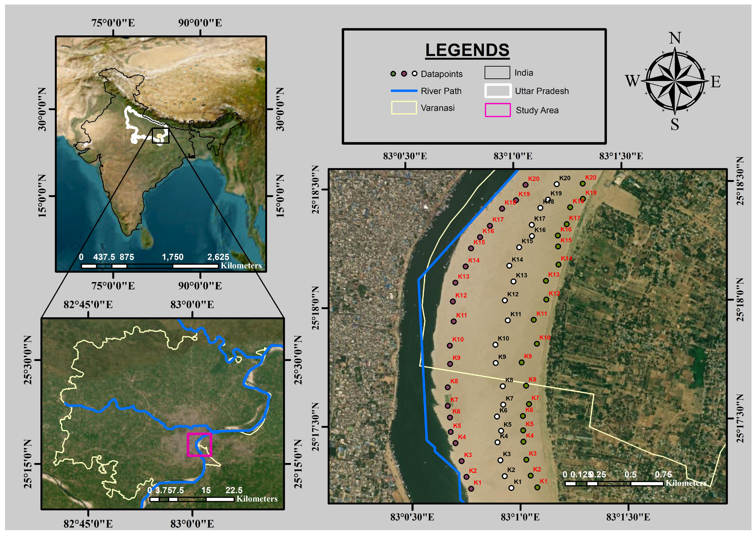
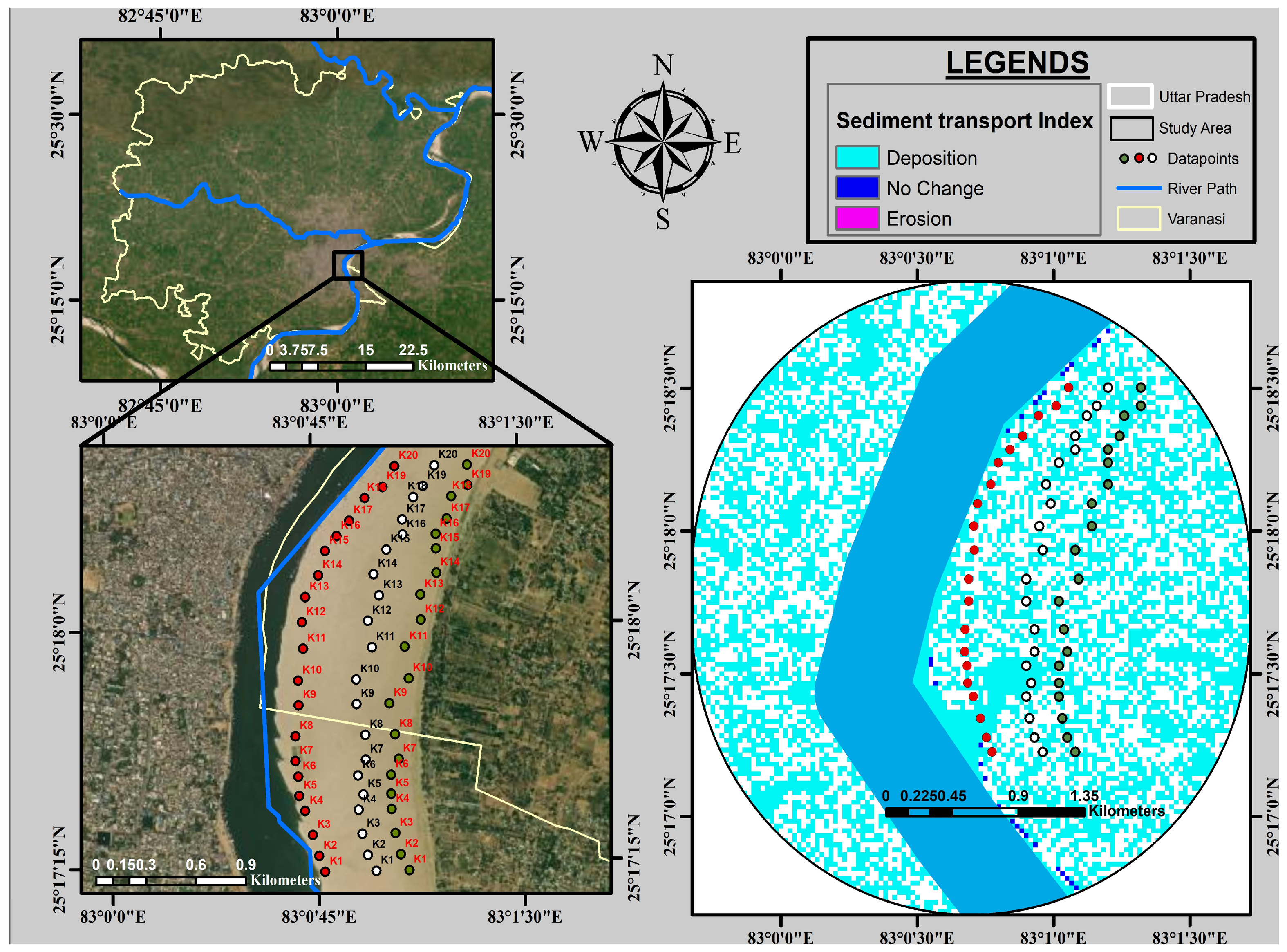
The climatic condition of the area is sub-tropical with temperatures varying between 5 °C in winters to 45 °C in summers [27]. The Ganga River is considered one of the most dynamic rivers of the Indian subcontinent and ranks amongst the major rivers in the world. The Ganga River, along with other rivers flowing in the northern and northeastern parts of India, create one of the largest deltas and a deep-sea fan with one of the thickest sedimentary sequences in the world. Around 729 × 10⁶ tons of sediment loads are transmitted annually to the Bay of Bengal through the Ganga River [27]. The city of Varanasi has long inspired researchers to conduct hydraulic studies on the Ganga River due to its unique flow pattern and channel geometry [27,28,29,30,31,32]. At this location, the Ganga River features two confluence points: the Assi River (rivulet) joins the Ganga at Assi Ghat, and the Varuna River converges with the Ganga at Sarai Mohana, approximately 5.7 km downstream from Assi Ghat [29]. Additionally, the Ganga River bends at this location, with the city of Varanasi situated on the outer convex bend, while the inner convex bend is characterized by sandbars and vegetation. Figure 1 illustrates the location of all 20 sampling stations on the right bank of the Ganga River at Varanasi. Approximately 2000 g of samples were collected from each station.

2.2. Grain Size Characters

Sieve analysis as per ASTM-C 136 [32] was conducted on 60 sand samples collected from the right bank of the Ganga River; these 60 samples were then grouped into 20 different sets and named k1 to k20, where each set comprised three distinct samples, as shown in Figure 1. The calculations were conducted by taking the average of three samples from each set. The samples were collected during pre-monsoon seasons (February–March 2024) as this period has a low incidence of peak flood events and the flow conditions are relatively steady.

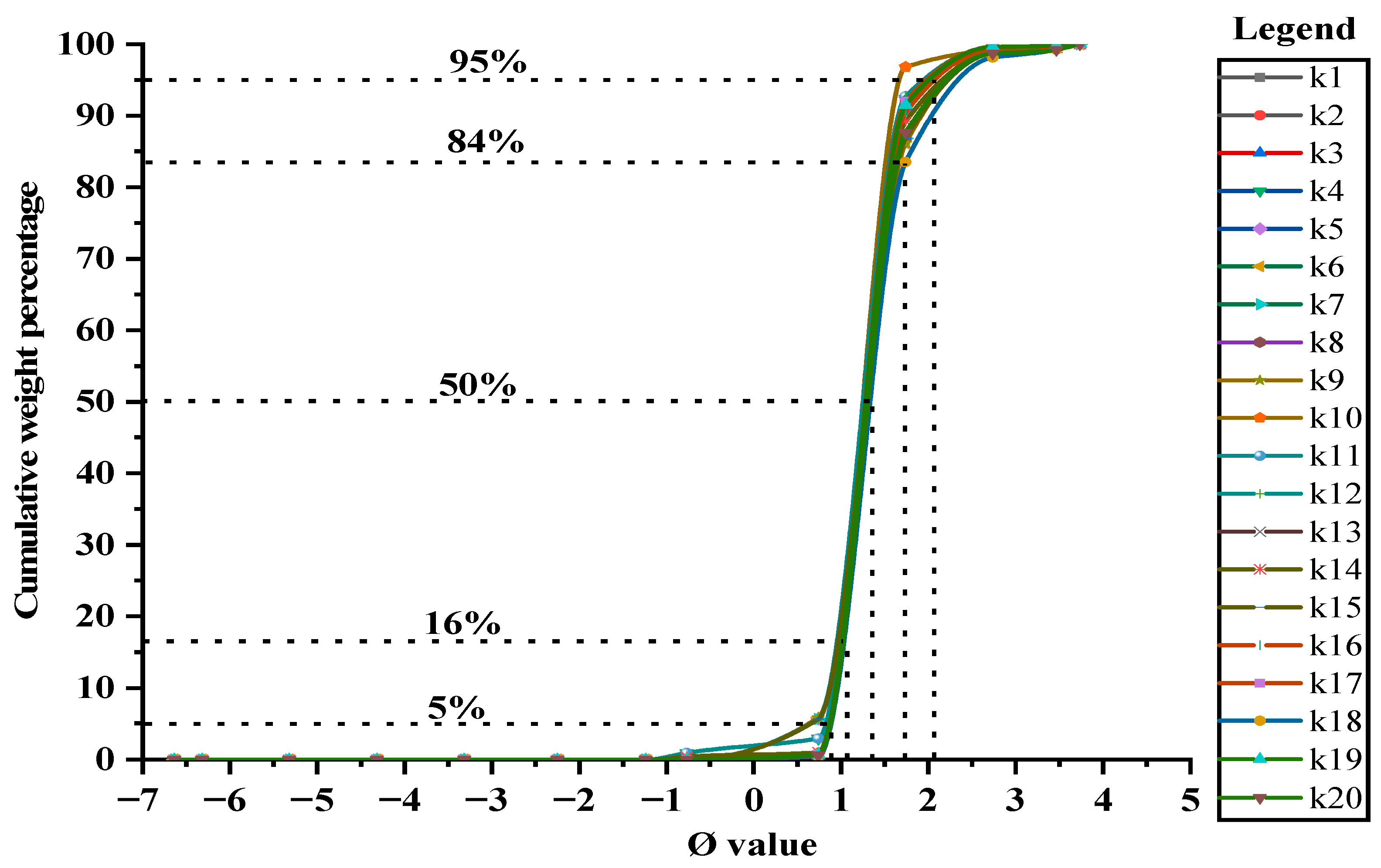
Before 2 kg of the sand sample by weight is utilized for the experiment, seven sieves of 2.36 mm, 1.18 mm, 600 μm, 300 μm, 150 μm, 90 μm, and 75 μm are arranged in order. The sieves are then stacked in the mechanical shaker and shaken for 15 min. The stack was then removed from the shaker, and the weight of each sieve with the retained sand was noted carefully. The cumulative values of the percentage of retained sand are calculated by dividing the weight retained on each sieve by the original sample weight. The ercentage of sediment passing through a particular sieve (or percentage finer) is calculated by cumulatively subtracting the percentage retained on each sieve from 100 percent. Figure 2 shows the cumulative percentage of sand retained vs. the $\varphi$ value logarithmic graph of river sand samples collected from all 20 sets.

Statistical parameters such as mean, standard deviation, skewness, and kurtosis of grain size distribution were computed and analyzed to highlight the characteristics of the deposited sediment particles. These parameters are calculated using the following equations, as has been suggested by Garde and Raju [5].

$$M_g={\displaystyle \frac{{\varphi }_{16}+{\varphi }_{50}+{\varphi }_{84}}{3}}$$

(1)

$${\sigma }_g={\displaystyle \frac{{\varphi }_{84}-{\varphi }_{16}}{4}}$$

(2)

$$S_K={\displaystyle \frac{{\varphi }_{84}+{\varphi }_{16}-2\left({\varphi }_{50}\right)}{2({\varphi }_{84}-{\varphi }_{16})}}+{\displaystyle \frac{{\varphi }_{95}+{\varphi }_5-2\left({\varphi }_{50}\right)}{2({\varphi }_{95}-{\varphi }_5)}}$$

(3)

$$K_G={\displaystyle \frac{{\varphi }_{95}-{\varphi }_5}{2.44({\varphi }_{75}-{\varphi }_{25})}}$$

(4)

$$\varphi =-{\mathit{log}}_2\left(D\right)$$

(5)

where ${\varphi }_5$, ${\varphi }_{16}$, ${\varphi }_{25}$, ${\varphi }_{50}$, ${\varphi }_{75}$, ${\varphi }_{84}$, and ${\varphi }_{95}$ represents the 5th, 16th, 25th, 50th, 75th, 84th, and 95th percentile, respectively, $\varphi$ is phi size, and D is grain diameter in millimetres. The negative sign denotes that sand sizes would have a positive $\varphi$ numbers. The base 2 logarithms follow the geometric Wentworth size scale [10].

In this study, grain size statistics are expressed using the graphical $\varphi$-percentile measures of Folk and Ward [11], although the same parameters can also be computed as exact moments of the full frequency distribution. Blott and Pye [33], showed that both graphical and moment methods have drawbacks, but for mean grain size and sorting, they usually give similar results. The graphical approach often provides a robust basis for comparison, particularly when skewness and kurtosis are also considered.

2.3. Linear Discriminate Function

Equation (6) was used to distinguish between shallow agitated water and beach, where if the value of Y₁ is less than −2.7411, the environment is said to be “aeolian”, and if Y₁ is greater than −2.7411, the environment is “beach”.

$$Y_1=-3.5688M_g+3.7016{{\sigma }_g}^2-2.0766S_K+3.1135K_G$$

(6)

Equation (7) was used to differentiate between beach and shallow agitated marine environments.

$$Y_2=15.6534M_g+65.7091{{\sigma }_g}^2+18.1071S_K+18.5043K_G$$

(7)

If Y₂ is less than 63.365, the environment is classified as “beach”. If Y₂ is greater than 63.3650, it is classified as “shallow agitated marine”. To distinguish between a “shallow marine” and a “deltaic or lacustrine” environment of deposition, Equation (8) was used:

$$Y_3=0.2852M_g-8.76046{{\sigma }_g}^2-4.8932S_K+0.0482K_G$$

(8)

The environment of deposition is said to be shallow marine if Y₃ is greater than −7.419. It is deltaic or lacustrine if the Y₃ value is less than −7.419. To discriminate between “deltaic” and “turbidity current” deposits, Equation (9) is utilized:

$$Y_4=0.7215M_g-0.4030{{\sigma }_g}^2+6.7322S_K+5.2927K_G$$

(9)

If Y₄ is less than 9.8433, the environment is classified as “turbidity current”. If Y₄ is greater than. 9.8433, it is classified as deltaic deposition.

The linear discriminant functions were originally developed by Sahu [17] using coastal, aeolian, and shallow-marine samples, and do not include alluvial river-bar sediments in their calibration.

2.4. Shear Stress Analysis

The calculations for available shear stress were done by Hager [34]:

$$\tau =\rho ghs$$

(10)

where $\rho$ is the water density (1.00 g/cm³), $g$ is the gravitational acceleration, h is the depth, and $s$ is the water surface slope whose value is calculated by using the equation suggested by Coon [35]. Flow depth (h) at each sampling station was measured in the field during the same pre-monsoon time when the samples were collected. Critical shear stress has been calculated by using the Shields [36] formula:

$${\tau }_C={\theta }^{*}(s-1)\rho g{d}_{50}$$

(11)

where ${\theta }^{*}$ is the dimensionless shields parameter (0.048), s is the specific gravity of the particle and is calculated as a ratio of the specific weight of the sediment $\left({\gamma }_s\right)$ to the specific weight of water $\left(\gamma \right)$ [37], and d₅₀ is the median grain size.

2.5. Sediment Transport Index (STI)

The sediment transport index (STI) provides information on sediment transport capacity, accumulation, and spatial distribution. STI is calculated as follows:

$$STI=\left\{(n+1){\left({\displaystyle \frac{A_s}{22.13}}\right)}^n\right\}\times \left\{{\left({\displaystyle \frac{sin\beta }{0.0896}}\right)}^m\right\}$$

(12)

where A_s is the flow accumulation, β is the slope obtained from the Digital Elevation Model (DEM), and n and m are constants whose values are 0.4 and 1.3, respectively.

In this study, STI is used as a hydrologic index of relative sediment transport potential and accumulation, not as a direct measure of bed shear stress or in-channel sediment flux. In the low-gradient Gangetic plains, STI values are therefore interpreted qualitatively to highlight zones of relatively higher or lower transport capacity across the bar-floodplain.

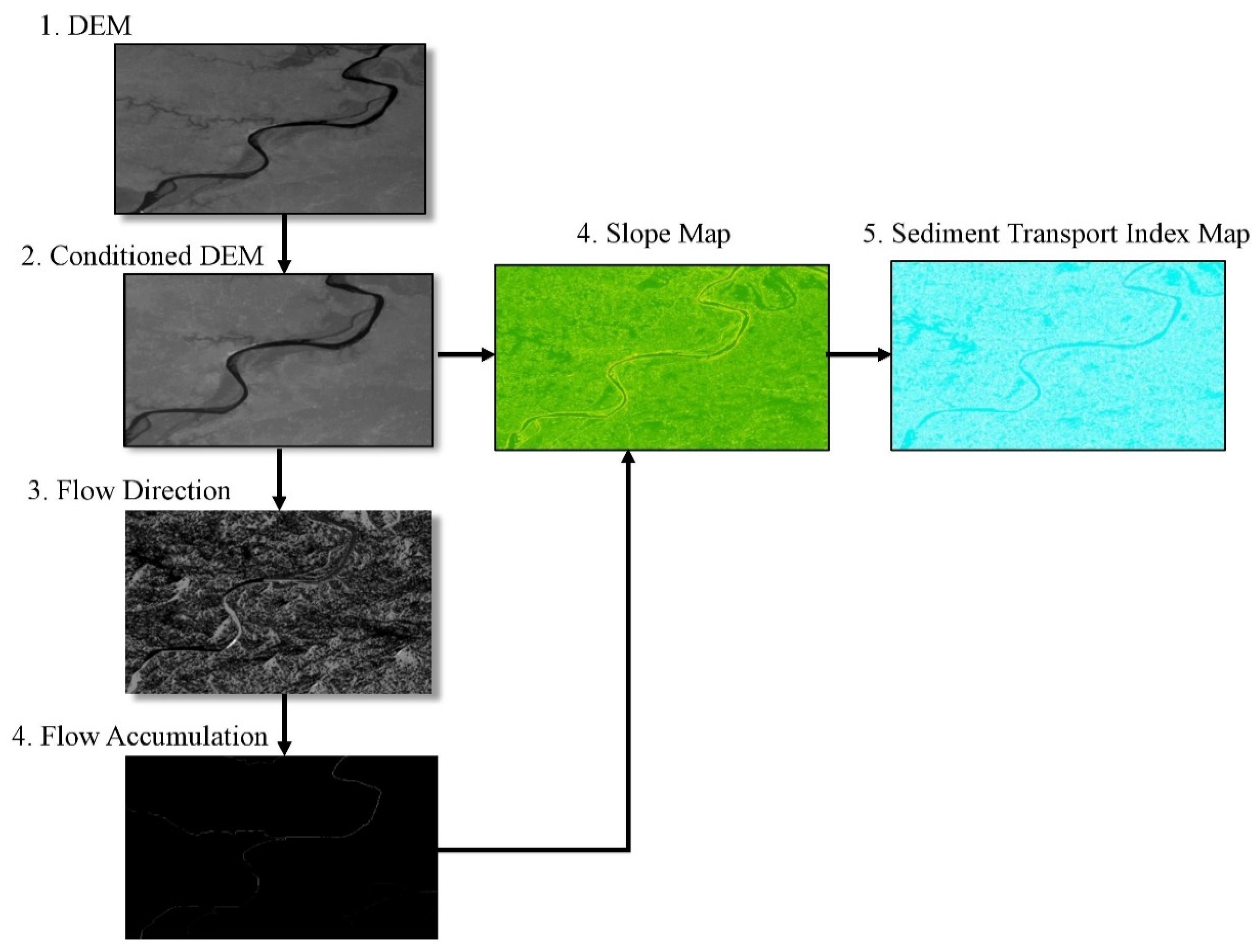
Figure 3 shows the complete flow chart of the methodology used during the formulation of STI. One arc-second (30 m × 30 m) Shuttle Radar Topography Mission (SRTM) DEM was used for the analysis of STI, and the following steps were taken to compute the value of STI over the study area:

• Filling sinks to generate conditioned DEM.
• Computation of flow direction
• Extraction of flow accumulation
• Generation of slope from conditioned DEM
• Computation of the STI using Equation (7)

3. Results

The result of this study not only focuses on the individual analysis of different parameters but also emphasizes the combined effect of each parameter to gain specific insights into various aspects of sediment characteristics. Mean grain size reveals the average size of sediment particles, which relates to the energy conditions and transport mechanisms of the depositional environment. Standard deviation measures the spread of sediment particles, indicating the uniformity and stability of transport conditions. Skewness shows the symmetry or asymmetry of the grain size distribution, providing insights into the energy level of the depositional environment. Kurtosis assesses the peakedness of the grain size distribution, offering clues about the sediment’s mixing and sorting history. However, the combined analysis of these parameters is essential for a comprehensive understanding of sediment nature and depositional settings. Correlating these parameters helps identify patterns and relationships that are not apparent in individual analyses, as the relationship between mean size and sorting can reveal transportation energy dynamics. Similarly, distinguishing between different environments, such as beach, shallow marine, and deltaic systems, can be achieved through a combined analysis of the interrelationships among various statistical parameters and using a linear differential approach.

Table 1. Observation table of statistical parameters calculated from the data of all 20 sampling stations.

S.No.	Station Code (k)	Mean (Mg)	Standard Deviation (σg)	Skewness (SK)	Kurtosis (KG)		S.No.	Station Code (k)	Mean (Mg)	Standard Deviation (σg)	Skewness (SK)	Kurtosis (KG)
1	k1	1.288	0.186	0.4	1.059		11	k11	1.264	0.189	0.3	0.969
2	k2	1.275	0.184	0.3	0.966		12	k12	1.250	0.195	0.2	1.069
3	k3	1.285	0.187	0.4	1.052		13	k13	1.288	0.188	0.5	1.071
4	k4	1.266	0.19	0.3	0.964		14	k14	1.295	0.193	0.5	1.131
5	k5	1.241	0.195	0.2	1.071		15	k15	1.286	0.209	0.4	1.233
6	k6	1.285	0.212	0.4	1.234		16	k16	1.289	0.189	0.5	1.077
7	k7	1.185	0.209	0.4	1.236		17	k17	1.280	0.186	0.4	1.007
8	k8	1.313	0.196	0.6	1.154		18	k18	1.347	0.213	0.7	1.179
9	k9	1.290	0.212	0.4	1.229		19	k19	1.282	0.187	0.4	1.026
10	k10	1.312	0.198	0.6	1.140		20	k20	1.308	0.196	0.6	1.150

summarizes the descriptive statistical parameters (mean, standard deviation, skewness, and kurtosis) calculated from the observed data at all 20 sampling stations.

3.1. Grain Size Characters

Observations drawn from this study show that the mean grain size ranges from ~1.185 to 1.347 in ϕ values, whereas other statistical parameters such as standard deviation, skewness, and kurtosis vary between ~0.184 to 0.213, ~0.2 to 0.7, and ~0.964 to 1.236, respectively. The results of the statistical parameters obtained from this study are provided in Table 1.

3.1.1. Mean (M_g)

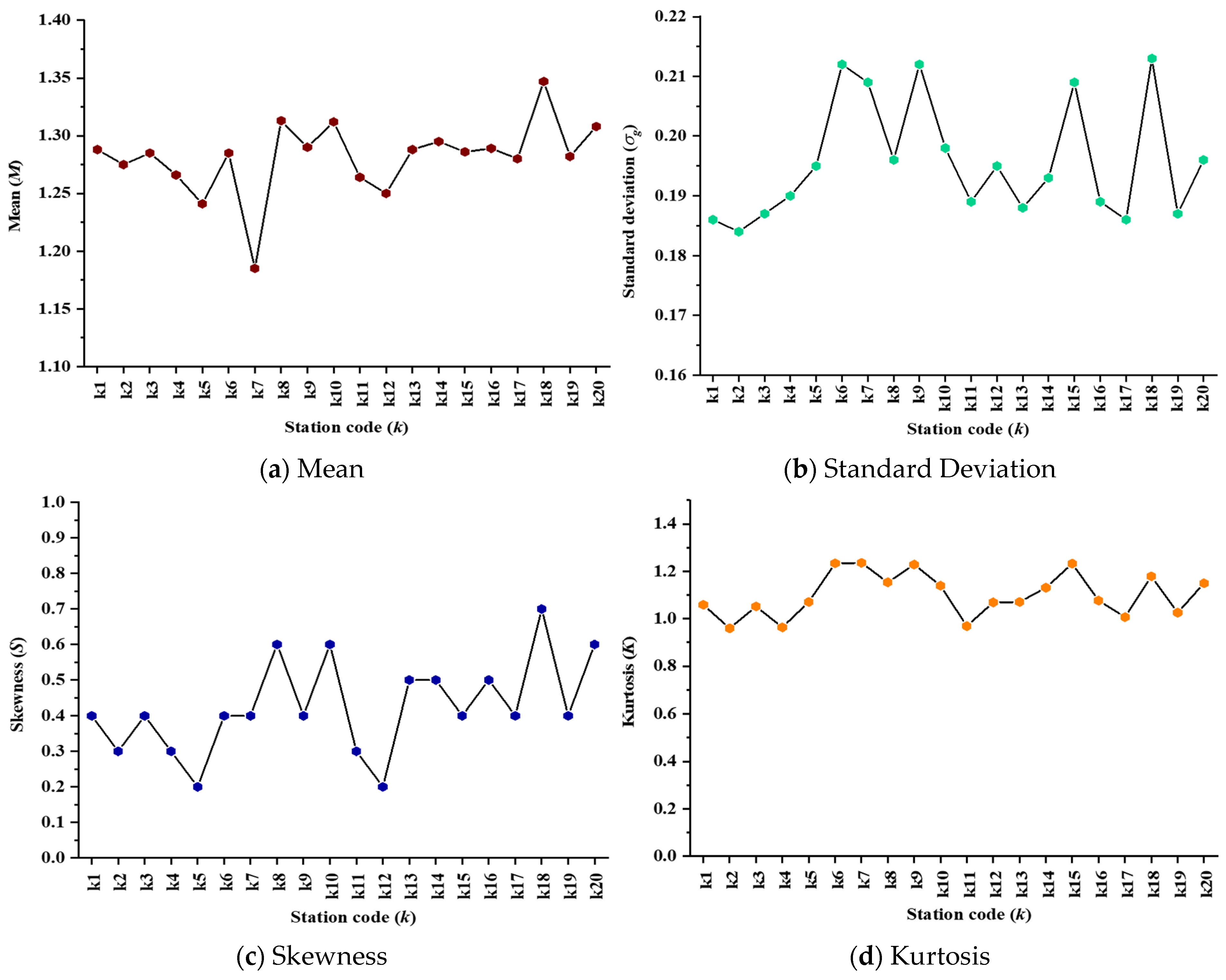
The distribution of mean grain size of the river sand particles collected from the study area lies in the range of ~1.185 to 1.347 (in $\varphi$ scale), as shown in Figure 4a, which clearly shows that the sand is medium-grained with values between 1.0 to 2.0 [10]. Factors that influence the mean size of sediments are the source of the supply, transporting medium, and energy conditions of the depositional environment [38,39].

3.1.2. Standard Deviation (σ_g)

As has been discussed earlier, standard deviation represents the measure of sorting in sediments. It also indicates fluctuations in the kinetic energy or velocity conditions of the depositing agent [17]. The difference in water turbulence and variability in the velocity of the depositing current also cause variation in the sorting values [40,41,42,43]. The standard deviation value for the collected sand samples lies in the range of ~0.184 to 0.213, as shown in Figure 4b.

Table 2. Sediment type sorting based on standard deviation range [33].

σg (in ϕ)	Degree of Sorting
Sorting less than 0.35	Very Well Sorted
0.35 to 0.50	Well Sorted
0.50 to 0.71	Moderately Well Sorted
0.71 to 1.00	Moderately Sorted
1.00 to 2.00	Poorly Sorted
2.00 to 4.00	Very Poorly Sorted
more than 4.00	Extremely Poorly Sorted

gives information about sediment type sorting based on the standard deviation range.

3.1.3. Skewness (S_K)

The symmetry or asymmetry of the frequency distribution of sediments is reflected by the skewness values. The sign possessed by the skewness value is related to environmental energy [44]. The skewness value for the collected samples falls in the range of fine to strongly fine skewed (~0.2 to 0.7) as shown in Figure 4c.

3.1.4. Kurtosis (K_G)

Kurtosis can offer insights into the mixing of sediment fractions, the history of sediment sorting, and bimodality sediment distribution sorting [11,45]. The sharpness and peakedness of the grain size distribution is highlighted by the kurtosis (see Figure 4d).

3.2. Dyadic Interrelationship of Statistical Parameters

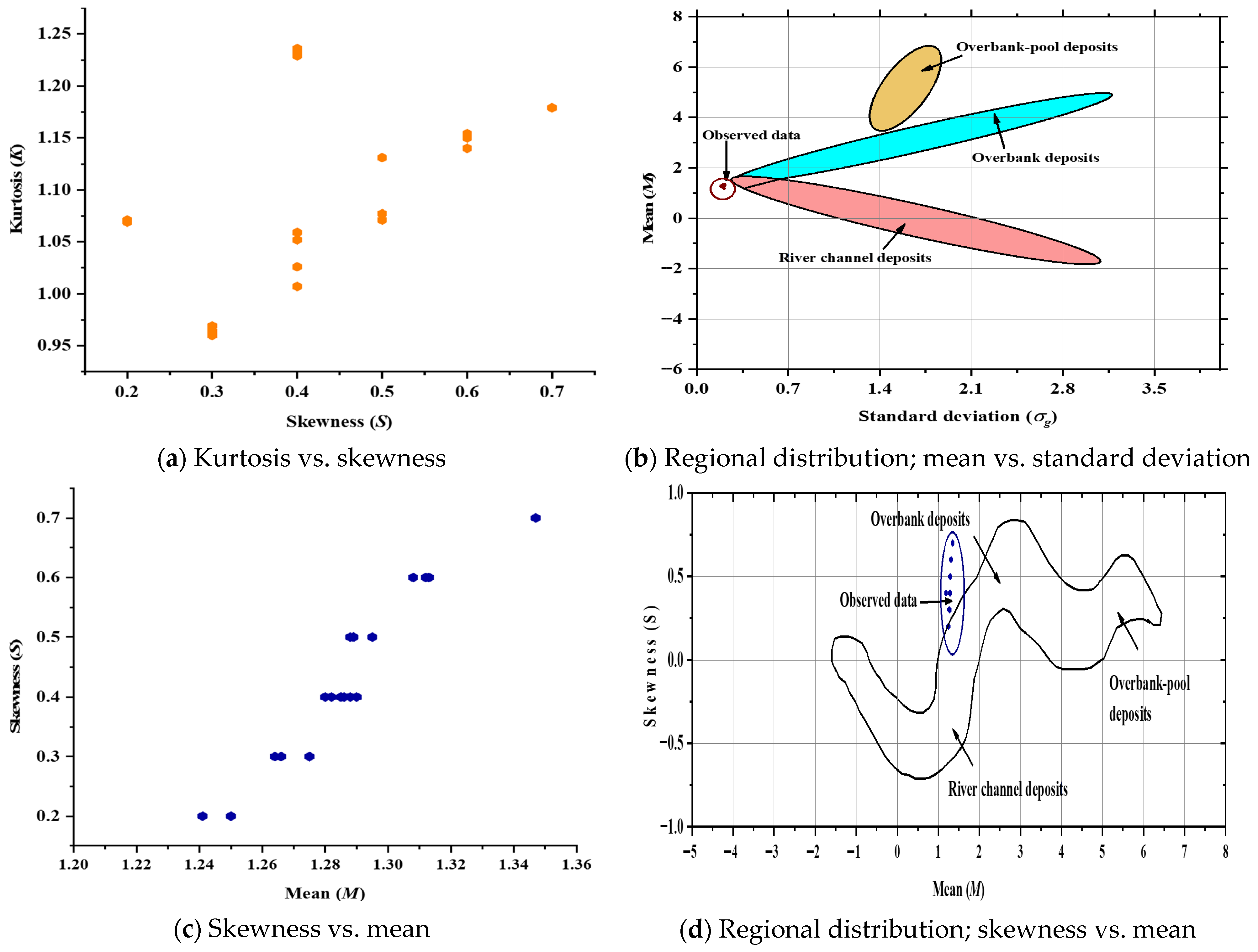
The interrelationship between the statistical parameters of sediments is plotted on a bivariate or dyadic graph. The characteristic properties of a fluvial process, such as mode of deposition, transportation medium, geological significance, and energy conditions can be revealed through these plots. Dyadic plots are also used to present the reliability of differences in the fluid flow and mechanism of sediment transport and deposition [46]. The transportation and deposition history of river sediments can be interpreted through the correlation of different granulometric parameters such as kurtosis vs. skewness, mean vs. standard deviation, standard deviation vs. skewness, and skewness vs. mean. These correlations are shown in Figure 5.

3.2.1. Kurtosis vs. Skewness

The kurtosis vs. skewness plot provides valuable insights into the sediment genesis, environmental conditions, and mixing processes. The observed value of skewness in the present study lies in the range of ~0.2 to 0.7 (shown in Figure 5a).

3.2.2. Mean vs. Standard Deviation

The standard deviation vs. mean plot gives insight into the sediment transport and prevailing energy condition. Sediments with a decreasing range of mean values typically indicate the influence of high-energy transport processes [47]. The plot of mean size against standard deviation is represented in Figure 5b. The plot reveals that the data points are clustered in well-sorted and fine-grained sediment and show a bimodal trend with a dominant constituent of sand.

3.2.3. Standard Deviation vs. Skewness

As standard deviation is a function of mean size, and it is evident that skewness is also a function of mean size, sorting and skewness will therefore also have a mathematical relation between them. Figure 5d shows that all the observed values are positively skewed, with the values indicating that most of the samples are strongly skewed toward fine particles and are very well sorted.

3.2.4. Skewness vs. Mean

Skewness is used as an indicator of sediment distribution, whereas mean indicates the variability of the sediments. The range of mean grain size (~1.185 to 1.347) and skewness (~0.2 to 0.7), as shown in Figure 5c, suggests that the sediment has a certain degree of variability in the grain size measurements.

3.3. Linear Discriminate Analysis

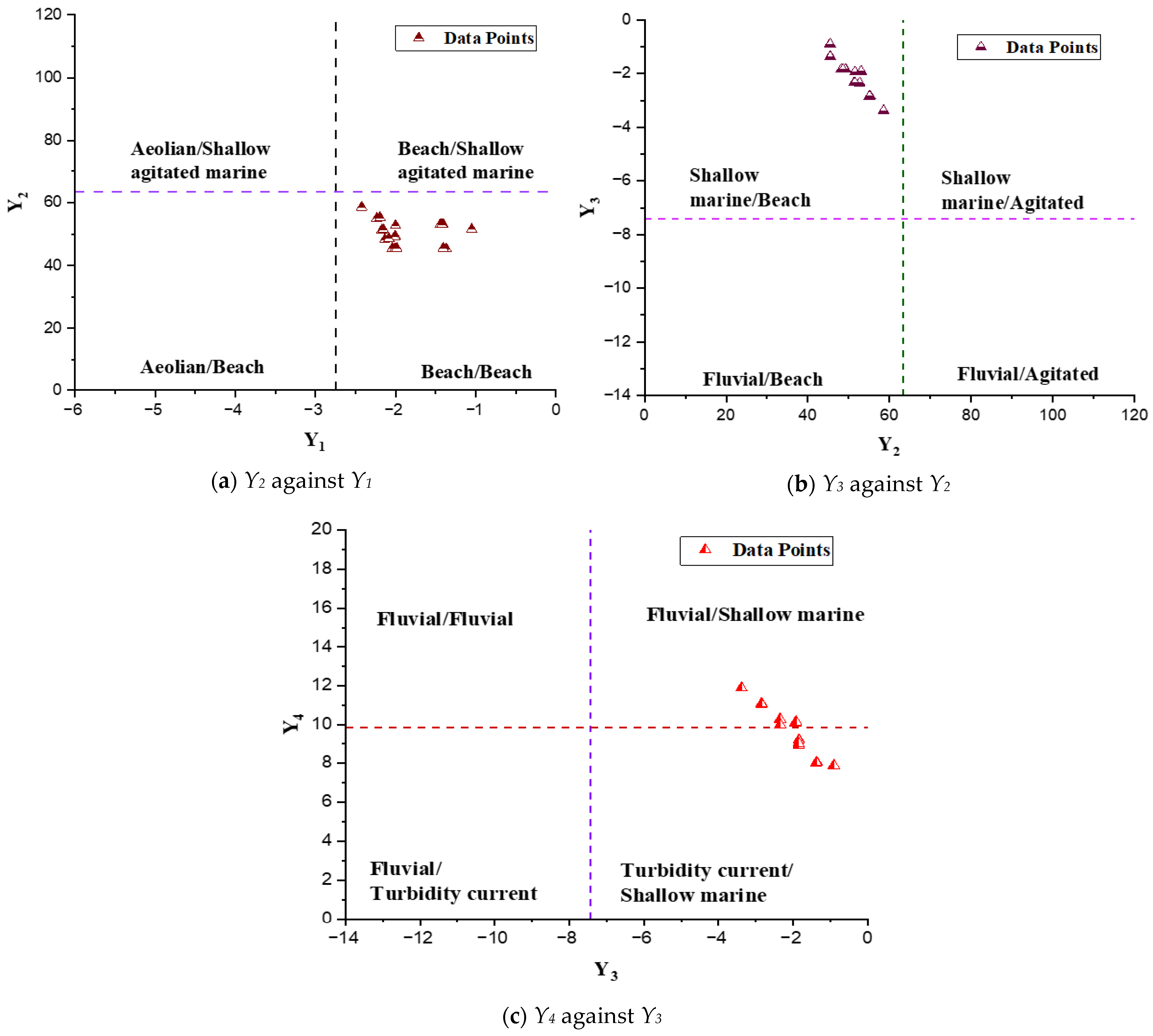
After analyzing the calculated values of the linear discriminant functions (LDF) presented in

Table 3. Linear discriminant function (LDF) values and depositional environments calculated after Sahu [17].

S.No.	Station Code (k)	Discriminant Function				Environment of Deposition
		Y1	Y2	Y3	Y4	Y1 Remarks	Y2 Remarks	Y3 Remarks	Y4 Remarks
1	k1	−2.002	49.273	−1.842	9.213	Beach	Beach	Shallow marine	Turbidity current deposition
2	k2	−2.040	45.490	−1.354	8.039	Beach	Beach	Shallow marine	Turbidity current deposition
3	k3	−2.012	49.121	−1.846	9.174	Beach	Beach	Shallow marine	Turbidity current deposition
4	k4	−2.006	45.459	−1.377	8.021	Beach	Beach	Shallow marine	Turbidity current deposition
5	k5	−1.369	45.363	−0.906	7.895	Beach	Beach	Shallow marine	Turbidity current deposition
6	k6	−1.408	53.144	−1.925	10.133	Beach	Beach	Shallow marine	Deltaic deposition
7	k7	−1.050	51.533	−1.942	10.072	Beach	Beach	Shallow marine	Deltaic deposition
8	k8	−2.197	55.295	−2.842	11.079	Beach	Beach	Shallow marine	Deltaic deposition
9	k9	−1.442	53.130	−1.924	10.110	Beach	Beach	Shallow marine	Deltaic deposition
10	k10	−2.234	55.072	−2.850	11.004	Beach	Beach	Shallow marine	Deltaic deposition
11	k11	−1.985	45.495	−1.374	8.046	Beach	Beach	Shallow marine	Turbidity current deposition
12	k12	−1.407	45.467	−0.904	7.891	Beach	Beach	Shallow marine	Turbidity current deposition
13	k13	−2.170	51.355	−2.337	9.950	Beach	Beach	Shallow marine	Deltaic deposition
14	k14	−2.001	52.700	−2.349	10.271	Beach	Beach	Shallow marine	Deltaic deposition
15	k15	−1.419	53.059	−1.914	10.129	Beach	Beach	Shallow marine	Deltaic deposition
16	k16	−2.153	51.507	−2.340	9.982	Beach	Beach	Shallow marine	Deltaic deposition
17	k17	−2.135	48.186	−1.847	8.932	Beach	Beach	Shallow marine	Turbidity current deposition
18	k18	−2.422	58.557	−3.382	11.906	Beach	Beach	Shallow marine	Deltaic deposition
19	k19	−2.082	48.593	−1.849	9.034	Beach	Beach	Shallow marine	Turbidity current deposition
20	k20	−2.191	55.143	−2.844	11.054	Beach	Beach	Shallow marine	Deltaic deposition

and Figure 6, a comprehensive understanding of the diverse depositional environment within the study area can be gathered. The depositional environments from the present study can be delineated as follows. Y₁, ranging from −1.04969 to −2.42204, indicates a depositional setting characterized as a “beach”. The values for Y₂, ranging from 58.55729 to 45.3634, again correspond to a “beach” environment. The “shallow marine” depositional setting is correlated by the value of Y₃, which ranges between −0.90373 to −3.3817. Lastly, the Y₄ values, ranging from 11.90621 to 7.890887, suggest a composite depositional environment influenced by both “deltaic” and “turbidity current”.

Descriptors such as “beach” and “shallow marine” are strictly used as grain size analogies for classification purposes, following Fridman [13]. These terms do not indicate actual marine processes at the site but serve to compare the sediment characteristics of the riverine samples with established depositional categories in sedimentology.

3.4. CM Diagram

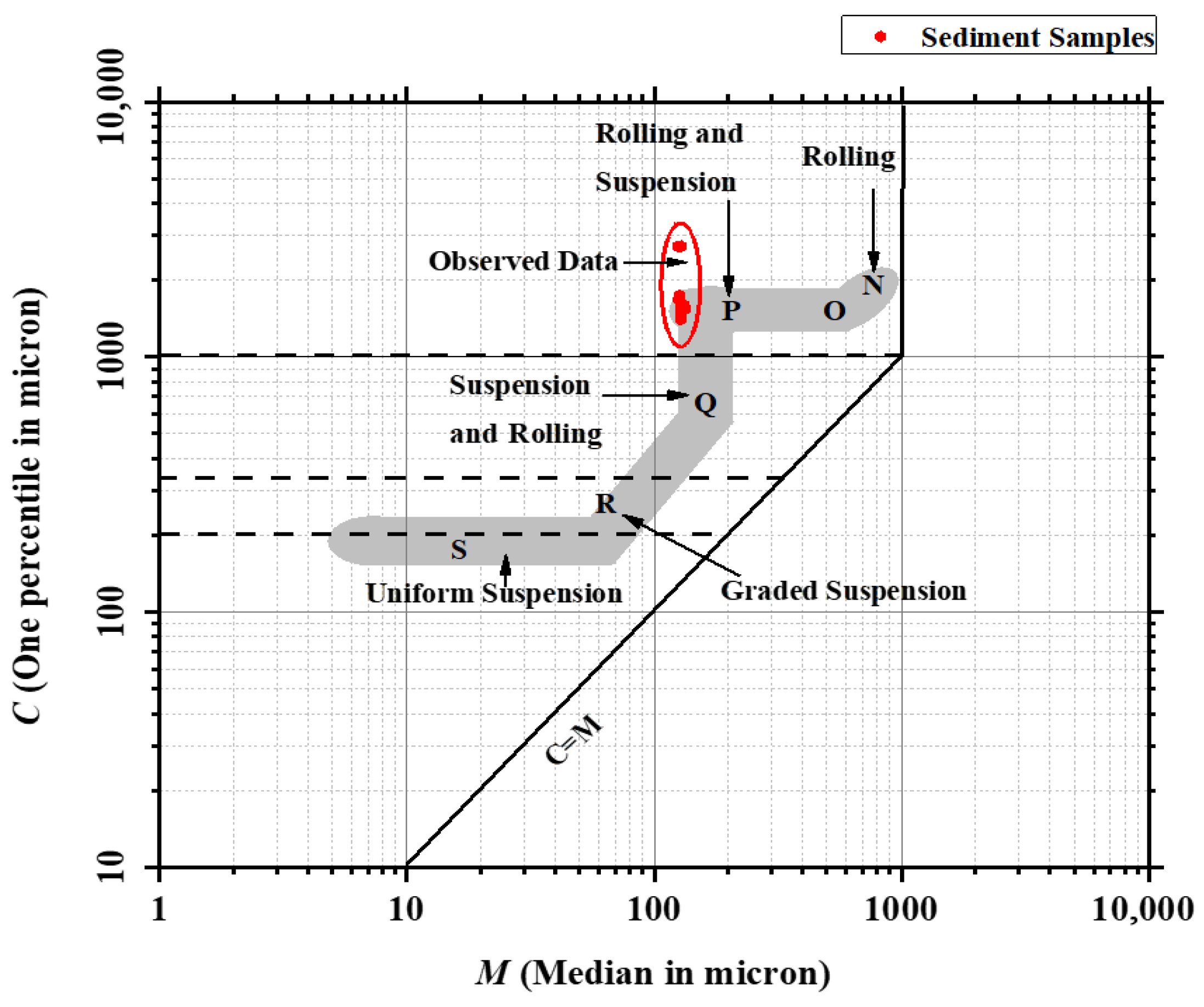
Passega [48] introduced the CM plot as a tool to evaluate hydrodynamic forces and sediment deposition. This plot represents the relationship between the coarser one percentile value (C) and the median value (M) of sediment samples on a log-probability scale. The interpretation of the CM plot reveals valuable insights into sedimentary processes and depositional environments [48,49,50]. The CM diagram as shown in Figure 7 represents various transport and sedimentation conditions such as rolling-NO, rolling and suspension-OP, suspension, rolling-PQ, graded suspension-QR, uniform suspension-RS, and pelagic suspension-T. The plot of the CM diagram in the present study describes that the collected sediments have rolling and suspension-OP modes of transportation.

3.5. Shear Stress

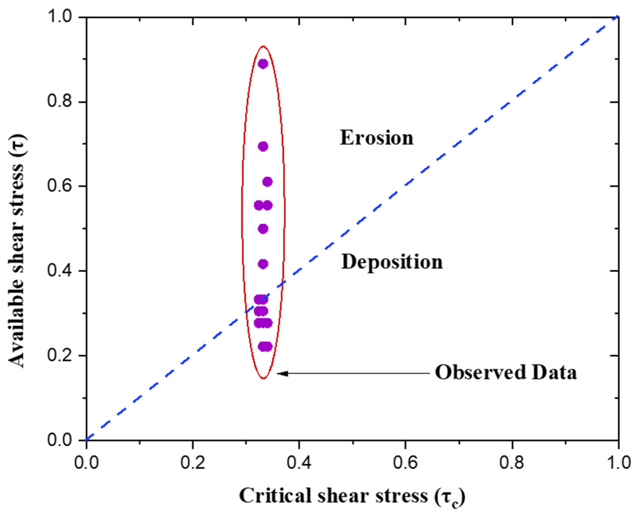
Figure 8 illustrates the relationship between available shear stress and critical shear stress, highlighting the threshold separating erosion and deposition regimes. Shear stress and its relationship with sediment transport dynamics are important for understanding the process of sediment erosion, deposition, and channel morphodynamics in river systems. Critical shear stress represents the minimum shear stress required to initiate particle entrainment and transport. When the shear stress exceeds the critical shear stress, sediment particles can be entrained and transported downstream, potentially leading to erosion and degradation of the riverbed or banks [20,21,22]. At lower shear stress, particles in contact with the bed roll or slide along the bed, and as shear stress increases, some particles lose contact with the bed and start to hop or bounce in the direction of flow. The presence of turbulence and fluctuation in flow can further lift the sand particles and transport them in suspension. This increase in shear stress can result in scouring action.

Table 4. Available and critical shear stress calculations.

S.No.	Station Code (k)	d50 Size (in m)	WSE (Sw)	τ (N/m2)	τc (N/m2)	Remarks
1	k1	0.00041	0.0000283	0.50	0.33	Erosion
2	k2	0.00041	0.0000283	0.28	0.33	Deposition
3	k3	0.00041	0.0000283	0.22	0.33	Deposition
4	k4	0.00042	0.0000283	0.22	0.34	Deposition
5	k5	0.00042	0.0000283	0.28	0.34	Deposition
6	k6	0.00041	0.0000283	0.28	0.33	Deposition
7	k7	0.00041	0.0000283	0.42	0.33	Erosion
8	k8	0.0004	0.0000283	0.33	0.32	Erosion
9	k9	0.00041	0.0000283	0.28	0.33	Deposition
10	k10	0.0004	0.0000283	0.56	0.32	Erosion
11	k11	0.00042	0.0000283	0.61	0.34	Erosion
12	k12	0.00042	0.0000283	0.56	0.34	Erosion
13	k13	0.00042	0.0000283	0.28	0.34	Deposition
14	k14	0.00041	0.0000283	0.69	0.33	Erosion
15	k15	0.00041	0.0000283	0.31	0.33	Deposition
16	k16	0.00041	0.0000283	0.89	0.33	Erosion
17	k17	0.00041	0.0000283	0.33	0.33	Erosion
18	k18	0.0004	0.0000283	0.31	0.32	Deposition
19	k19	0.00041	0.0000283	0.28	0.33	Deposition
20	k20	0.0004	0.0000283	0.28	0.32	Deposition

lists the median grain size (d₅₀), water-surface slope, and the corresponding available shear stress for all 20 stations under the measured pre-monsoon flow condition. The table also provides the calculated value of available and critical shear stress at the locations of the study area. These values form the basis for the erosion–deposition assessment shown in Figure 8.

3.6. Sediment Transport Index

The analysis of the sediment transport index (STI) reflects a lower value throughout the observation sites, as shown in Figure 9, which corresponds to landforms composed of terrains with flat slope or features such as basaltic rocks. These possess high hardness and exhibit minimal erosion and considerable depositional characteristics. Such landforms exhibit resilience against erosive forces, making them resistant to significant soil erosion and degradation. Consequently, the flow in these areas can cause lower erosion rates.

Overall, the study employs a novel use of the linear discriminant function (LDF) to assess the energy, fluidity, and environmental factors related to sediment deposition. The findings showed different depositional environments: shallow marine settings are suggested by Y₃ values, whereas beach environments are indicated by Y₁ and Y₂ values. The Y₄ readings show that the current depositional conditions are a mixture of turbid and deltaic.

An analysis of sediment sample data utilizing a CM diagram, the coarser one percentile value (C), and the median value (M) on a log-probability scale revealed that, at a particular research location, sand deposition is mostly caused by rolling and suspension mechanisms. Furthermore, the plot shows shear stress against critical shear stress, which suggests that deposition is common over a sizable amount of the research region. Using the sediment transport index (STI) to provide an additional perspective on sediment mobility under local topographic and flow conditions showed that the study area has significant depositional characteristics. The use of STI in this study is exploratory and results are interpreted cautiously, acknowledging that STI may have limitations in large, low-gradient fluvial systems.

4. Discussion

This section interprets the results linking them to the study objectives, research, and the broader context of the sediment dynamics in the Ganga River at Varanasi. The combined results fulfill the study objectives by elucidating grain size characteristics, transport mechanism (rolling and suspension), and depositional environments (beach, shallow marine, deltaic–turbid mix). The low energy condition inferred from statical parameters LDF, and STI aligns with the Ganga River bend at Varanasi, where sediment accumulated due to reduced flow velocity and topographic influences.

4.1. Grain Size Characters and Statistical Parameters

The medium-grained sand sample from the present study indicates a source of moderately weathered parent rocks, likely transported by fluvial or aeolian processes. This also suggests deposition in a quiet water environment, such as slow-moving rivers, floodplains, or a protected aeolian setting, characterized by moderate energy conditions that effectively sort and deposit medium size grains. The depositional setting had sufficient energy to transport and deposit sand-sized particles while preventing the accumulation of significantly finer or coarser sediments. Table 2 gives information about sediment type classification based on the mean range. The mean grain size of sand samples collected from the study area suggests higher kinetic energy and velocity of the depositional agent [51]. The soil sample used for the study can be categorized as very well sorted, as the standard deviation value lies under 0.35, suggesting a uniform source and consistent transport conditions. This points to depositional environments with stable energy levels. The results of skewness observed in the present study indicate that the sand samples are deposited in low- to moderate-energy environments where finer particles are preferentially deposited. This suggests stable conditions conducive to the accumulation of fine-grained sediments such as lagoons, protected bays, and lower energy fluvial environments. Figure 4c gives information about the symmetry of distribution based on the skewness range. This nature of skewness suggests that a major part of the sediment is skewed towards the coarser side, due to which sediments are deposited with minimum erosion effect. Figure 4d gives information about the tailedness of the distribution based on the kurtosis range. At stations k6, k7, and k9 the value of kurtosis shows a considerably leptokurtic distribution, suggesting a relatively uniform sediment population with little variation in grain size, whereas stations k2, k4, and k11 have a considerable mesokurtic distribution, suggesting that there is a balanced mixture of different grain sizes without a dominant mode.

4.2. Dyadic Interrelationship of Statical Parameters

The result from the kurtosis vs. skewness plot indicates that the distribution is skewed towards larger (coarse) grain size, while the values of kurtosis suggest a moderately concentrated distribution around the mean. The combination of coarser skewness and moderately peaked kurtosis suggests that the sediment deposit is influenced by a low-energy process with a uniform sediment population. The mean vs. standard deviation graph demonstrates that sorting values are higher at stations where the computed mean is higher, as the mean grain size and sorting characteristics are controlled by stream hydraulics. The standard deviation vs. mean graph has two fields, as shown in Figure 5c, representing over-bank deposits and river channel deposits. The standard deviation value on the horizontal axis of Figure 5c shows that the sediment particles are under the category of very well sorted, as the observed data falls in the range of ~0 to 0.3, and at the same time the vertical axis representing the mean shows that the sediment particles are medium grained, as the value of the mean falls in the range from ~1 to 2. The combined observation drawn from the mean vs. standard deviation curve shows that sediment particles are part of a riverbank deposit. Figure 5c also has an overlapping field of points at mean ~2ϕ, which corresponds to the best-sorted grain size. The standard deviation vs. skewness plot suggests that the observed value tends to have a fine particle tail indicating an excess of larger (coarser) grains to mean size. The positive skewness and sorting values reveal that the observed values are in a low-energy environment [44]. The finer particle tail observed in the skewness vs. mean plot indicates that the sediment sample tends to contain relatively more coarse-grained particles. The observed data in Figure 5c suggest that with an increase in the value of average grain size or mean, the skewness value also increases. The positive skewed value indicates that the sediments may have been deposited in a low-energy environment where fine particles tend to settle out first [44].

4.3. Depositional Environments from Linear Discriminant Analysis

The plot of Y₂ against Y₁ shows that most of the samples from the sand bar at the bend of the Ganga River at Varanasi lie in the “Beach” depositional setting, as shown in Figure 6a. This might be explained by the higher skewness value of the sample collected in the present study when compared to the study of Singh et al. [27]. The higher skewness value corresponds to the low energy transport medium, or in other words, it indicates a depositional environment like rivers in areas with slow flow rates, floodplains, or aeolian settings such as dunes, where finer sediments are prevalent. The topography and unidirectional flow of the bend of the Ganga River at Varanasi and the river bar where all the samples are collected also reflect the same deposition. The plot of Y₃ against Y₂, as shown in Figure 6b, indicates that all the samples from the site are in shallow marine/beach environments. Figure 6c shows the plot of Y₄ against Y₃ where a mix of both deltaic and turbidity current depositional environments is highlighted.

4.4. Sediment Transport Mechanism from CM Diagram

The CM diagram in Figure 7 shows rolling and suspension as the dominant transport mechanism, which consistent with a low to moderate energy fluvial system where sediment moves along the bed or is briefly suspended during the flow fluctuation [50]. This supports the grain size and skewness findings of minimal erosion and stable deposition.

4.5. Shear Stress and Erosion Deposition Dynamics

During the period of high stress, such as monsoon season, the shear stress exceeds the critical shear stress, causing sediment to be easily entrained and transported downstream. This results in significant scouring of riverbeds and erosion of banks. Calculations for available shear stress and critical shear stress values are shown in Figure 8, which clearly shows the dominance of sediment deposition over the study area, as more than 60% of the observation sites show sediment deposition.

4.6. Sediment Transport Index (STI) and Geospatial Analysis

Low SIT values, as shown in Figure 9, across the study area suggest minimal erosion potential, consistent with flat terrain or resistant geological features [23]. This corroborates the shear stress and grain size findings, indicating that a stable deposition prone environment and limited sediment flux align with the river bend’s geomorphological context.

4.7. Limitations and Future Research

While this study provides valuable insights into sediment transport dynamics in the Ganga River at Varanasi, several limitations must be acknowledged. These constraints affect the interpretation and generalizability of the findings. Addressing them in future research will help build a more complete understanding of the riverine sediment process.

• Samples were limited to a small portion of the river near Varanasi. Broader coverage would improve understanding of spatial variability.
• Data was collected during a single period, so seasonal or event-based changes in sediment transport were not captured.
• The study did not incorporate high-resolution GIS and remote sensing data for detailed mapping.
• STI and related LS indices were developed for hillslopes; their quantitative accuracy in large, low-slope rivers is limited.
• Future studies can explore broader impacts, such as ecological changes and pollutant transport.
• Recalibrated LDF analysis using datasets that include river sands can be employed by integrating machine learning techniques, “river–beach–delta discrimination model.”

5. Conclusions

This study provides valuable insights into the sediment dynamics of the Ganga River at Varanasi by integrating statistical grain size analysis and geospatial assessment. Our results demonstrate that sediments in the study area are predominantly medium-grained and well sorted, indicating consistency in sediment supply and the influence of steady, low-energy hydrodynamic conditions. The statistical evaluation supports the interpretation that energy fluctuations in the river bend are minimal, leading to efficient sorting and stable deposition patterns.

Discriminant function and statistical relationships point towards a depositional environment shaped by a combination of fluvial, shallow marine, and aeolian (wind-driven) processes, highlighting the interplay between riverine flows and occasional wind or tidal actions. Modes of transport inferred from sediment analysis where primarily rolling and suspension underscore the prevalence of gentle, gradual deposition. The calculated values of the shear stress and sediment transport indices further confirm the dominance of deposition over erosion in the river. Among the various analytical approaches used, statistical grain size analysis and discriminant function modeling proved most effective for characterizing the sedimentary environment and its processes in the study area.

The application of shear stress calculation and sediment transport indices offered targeted insights into current deposition dynamics, validating the relevance of these metrics for large alluvial rivers such as the Ganga. Furthermore, spatial analysis of grain size and sediment transport indices across the sampled station revealed some patterns of local variability. These comparisons between sampled sites highlight the difference in the sedimentary processes within the study area, offering a more nuanced understanding of factors controlling deposition and erosion.

References

1. Boggs, S. Principles of Sedimentology and Stratigraphy; Pearson: London, UK, 2012. [Google Scholar]
2. Allen, J.R. A review of the origin and characteristics of recent alluvial sediments. Sedimentology 1965, 5, 89–191. [Google Scholar] [CrossRef]
3. Coleman, J.M. Brahmaputra River: Channel processes and sedimentation. Sediment. Geol. 1969, 3, 129–239. [Google Scholar] [CrossRef]
4. Whetten, J.T.; Kelley, J.C.; Hanson, L.G. Characteristics of Columbia River sediment and sediment transport. J. Sediment. Res. 1969, 39, 1149–1166. [Google Scholar] [CrossRef]
5. Garde, R.J.; Raju, K.R. Mechanics of Sediment Transportation and Alluvial Stream Problems; Taylor & Francis: Oxfordshire, UK, 2000. [Google Scholar]
6. Knighton, A.D. Longitudinal changes in size and sorting of stream-bed material in four English rivers. Geol. Soc. Am. Bull. 1980, 91, 55–62. [Google Scholar] [CrossRef]
7. Brierley, G.J.; Hickin, E.J. The downstream gradation of particle sizes in the Squamish River, British Columbia. Earth Surf. Process. Landf. 1985, 10, 597–606. [Google Scholar] [CrossRef]
8. Bridge, J.S.; Smith, N.D.; Trent, F.; Gabel, S.L.; Bernstein, P. Sedimentology and morphology of a low-sinuosity river: Calamus River, Nebraska Sand Hills. Sedimentology 1986, 33, 851–870. [Google Scholar] [CrossRef]
9. Bilal, A.; Yang, R.; Chen, S.; Lenhardt, N.; Mughal, M.S.; Kontakiotis, G. Seismically induced Soft-Sediment deformation in alluvial Fans: Mechanisms and Implications for geological evolution of the Ordos Basin (China). J. Asian Earth Sci. 2025, 294, 106821. [Google Scholar] [CrossRef]
10. Krumbein, W.C. Size frequency distributions of sediments and the normal phi curve. J. Sediment. Res. 1938, 8, 84–90. [Google Scholar] [CrossRef]
11. Folk, R.L.; Ward, W.C. Brazos River bar [Texas]; a study in the significance of grain size parameters. J. Sediment. Res. 1957, 27, 3–26. [Google Scholar] [CrossRef]
12. Friedman, G.M. On sorting, sorting coefficients, and the lognormality of the grain-size distribution of sandstones. J. Geol. 1962, 70, 737–753. [Google Scholar] [CrossRef]
13. Friedman, G.M. Dynamic processes and statistical parameters compared for size frequency distribution of beach and river sands. J. Sediment. Res. 1967, 37, 327–354. [Google Scholar] [CrossRef]
14. Martins, L.R. Significance of skewness and kurtosis in environmental interpretation. J. Sediment. Res. 1965, 35, 768–770. [Google Scholar] [CrossRef]
15. Moiola, R.J.; Weiser, D. Textural parameters; an evaluation. J. Sediment. Res. 1968, 38, 45–53. [Google Scholar]
16. Mueller, E.R.; Pitlick, J.; Nelson, J.M. Variation in the reference Shields stress for bed load transport in gravel-bed streams and rivers. Water Resour. Res. 2005, 41, W04006. [Google Scholar] [CrossRef]
17. Sahu, B.K. Depositional mechanisms from the size analysis of clastic sediments. J. Sediment. Res. 1964, 34, 73–83. [Google Scholar] [CrossRef]
18. Rajganapathi, V.C.; Jitheshkumar, N.; Sundararajan, M.; Bhat, K.H.; Velusamy, S. Grain size analysis and characterization of sedimentary environment along Thiruchendur coast, Tamilnadu, India. Arab. J. Geosci. 2013, 6, 4717–4728. [Google Scholar] [CrossRef]
19. Baiyegunhi, C.; Liu, K.; Gwavava, O. Grain size statistics and depositional pattern of the Ecca Group sandstones, Karoo Supergroup in the Eastern Cape Province, South Africa. Open Geosci. 2017, 9, 554–576. [Google Scholar] [CrossRef]
20. Buffington, J.M.; Montgomery, D.R. A systematic analysis of eight decades of incipient motion studies, with special reference to Gravel-bedded Rivers. Water Resour. Res. 1997, 33, 1993–2029. [Google Scholar] [CrossRef]
21. Church, M. Bed material transport and the morphology of alluvial river channels. Annu. Rev. Earth Planet. Sci. 2006, 34, 325–354. [Google Scholar] [CrossRef]
22. Charlton, R. Fundamentals of Fluvial Geomorphology; Routledge: New York, NY, USA, 2007; p. 234. [Google Scholar]
23. Moore, I.D.; Wilson, J.P. Length-slope factors for the Revised Universal Soil Loss Equation: Simplified method of estimation. J. Soil Water Conserv. 1992, 47, 423–428. [Google Scholar] [CrossRef]
24. Wischmeier, W.H.; Smith, D.D. Predicting Rainfall Erosion Losses: A Guide to Conservation Planning; Department of Agriculture, Science and Education Administration: Washington, DC, USA, 1978.
25. Desmet, P.J.J.; Govers, G. A GIS procedure for automatically calculating the USLE LS factor on topographically complex landscape units. J. Soil Water Conserv. 1996, 51, 427–433. [Google Scholar] [CrossRef]
26. Whitehead, P.G.; Sarkar, S.; Jin, L.; Futter, M.N.; Caesar, J.; Barbour, E.; Leckie, H.D. Dynamic modeling of the Ganga river system: Impacts of future climate and socio-economic change on flows and nitrogen fluxes in India and Bangladesh. Environ. Sci. Process. Impacts 2015, 17, 1082–1097. [Google Scholar] [CrossRef]
27. Singh, M.; Singh, I.B.; Müller, G. Sediment characteristics and transportation dynamics of the Ganga River. Geomorphology 2007, 86, 144–175. [Google Scholar] [CrossRef]
28. Chauhan, M.S.; Dikshit, P.K.S.; Dwivedi, S.B. Modeling of Discharge Distribution in Bend of Ganga River at Varanasi. Comput. Water Energy Environ. Eng. 2015, 4, 25. [Google Scholar] [CrossRef][Green Version]
29. Chauhan, M.S.; Kumar, V.; Rahul, A.K.; Dikshit, P.K.S.; Dwivedi, S.B. Spatial distribution of the suspended sediments in River Ganga at Varanasi, Uttar Pradesh, India. Int. J. Earth Sci. Eng. 2017, 10, 533–540. [Google Scholar]
30. Shivhare, N.; Rahul, A.K.; Dwivedi, S.B.; Dikshit, P.K.S. ARIMA based daily weather forecasting tool: A case study for Varanasi. Mausam 2019, 70, 133–140. [Google Scholar] [CrossRef]
31. Rahul, A.K.; Shivhare, N.; Kumar, S.; Dwivedi, S.B.; Dikshit, P.K.S. Modelling of daily suspended sediment concentration using FFBPNN and SVM algorithms. J. Soft Comput. Civ. Eng. 2021, 5, 120–134. [Google Scholar]
32. ASTM C136-06; Standard Test Method for Sieve Analysis of Fine and Coarse Aggregates. ASTM: West Conshohocken, PA, USA, 1984.
33. Blott, S.J.; Pye, K. GRADISTAT: A grain size distribution and statistics package for the analysis of unconsolidated sediments. Earth Surf. Process. Landf. 2001, 26, 1237–1248. [Google Scholar] [CrossRef]
34. Hager, W.H. Du Boys and sediment transport. J. Hydraul. Res. 2005, 43, 227–233. [Google Scholar] [CrossRef]
35. Coon, W.F. Estimation of Roughness Coefficients for Natural Stream Channels with Vegetated Banks; US Geological Survey: Reston, VA, USA, 1998; Volume 2441.
36. Shields, A. Anwendung der Aehnlichkeitsmechanik und der Turbulenzforschung auf die Geschiebebewegung. Mitteilungen Der Preuss. Vers. Für Wasserbau Und Schiffbau 1936, 26, 5. [Google Scholar]
37. Berenbrock, C.; Tranmer, A.W. Simulation of Flow, Sediment Transport, and Sediment Mobility of the Lower Coeur d’Alene River, Idaho; Geological Survey: Reston, VA, USA, 2008.
38. Visher, G.S. Grain size distributions and depositional processes. J. Sediment. Res. 1969, 39, 1074–1106. [Google Scholar] [CrossRef]
39. Sly, P.G.; Thomas, R.L.; Pelletier, B.R. Comparison of sediment energy-texture relationships in marine and lacustrine environments. Hydrobiologia 1982, 91, 71–84. [Google Scholar] [CrossRef]
40. Ramanathan, A.L.; Rajkumar, K.; Majumdar, J.; Singh, G.; Behera, P.N.; Santra, S.C.; Chidambaram, S. Textural Characteristics of the Surface Sediments of a Tropical Mangrove Sundarban Ecosystem India; CSIR: New Delhi, India, 2009. [Google Scholar]
41. Rajamanickam, G.V.; Gujar, A.R. Indications given by median distribution and CM patterns on clastic sedimentation in Kalbadevi, Mirya and Ratnagiri bays, Maharashtra, India. G. Geol. 1985, 47, 237–251. [Google Scholar]
42. Rajamanickam, G.V.; Muthukrishnan, N. Grain size distribution in the Gadilam river basin, northern Tamil Nadu. J. Indian Assoc. Sedimentol. 1995, 14, 55–66. [Google Scholar]
43. Angusamy, N.; Rajamanickam, G.V. Depositional environment of sediments along the southern coast of Tamil Nadu, India. Oceanologia 2006, 48, 87–102. [Google Scholar]
44. Duane, D.B. Significance of skewness in recent sediments, western Pamlico Sound, North Carolina. J. Sediment. Res. 1964, 34, 864–874. [Google Scholar] [CrossRef]
45. Folk, R.L. A review of grain-size parameters. Sedimentology 1966, 6, 73–93. [Google Scholar] [CrossRef]
46. Sutherland, R.A.; LEE; CT. Discrimination between coastal subenvironments using textural characteristics. Sedimentology 1994, 41, 1133–1145. [Google Scholar] [CrossRef]
47. Bhattacharya, R.K.; Das Chatterjee, N.; Dolui, G. Grain size characterization of instream sand deposition in controlled environment in river Kangsabati, West Bengal. Model. Earth Syst. Environ. 2016, 2, 118. [Google Scholar] [CrossRef]
48. Passaga, R. Textural as characteristics of clastic deposition. Bull. Am. Assoc. Pet. Geol. 1957, 41, 1952–1984. [Google Scholar]
49. Passega, R. Grain size representation by CM patterns as a geologic tool. J. Sediment. Res. 1964, 34, 830–847. [Google Scholar] [CrossRef]
50. Passega, R.; Byramjee, R. Grain-size image of clastic deposits. Sedimentology 1969, 13, 233–252. [Google Scholar] [CrossRef]
51. Htun, M.M.; Surjono, S.S.; Setyowiyoto, J. Granulometry analysis of Ngrayong sandstone, Tempuran Area, Rembang Zone, North East Java Basin. In IOP Conference Series: Earth and Environmental Science; IOP Publishing: Bristol, UK, 2020; Volume 451, p. 012082. [Google Scholar]
Figure 1. Study area and the locations of all the 20 sampling sites.
Earth 07 00011 g001
Figure 2. Cumulative percentage sand retained vs. the ϕ value logarithmic graph of river sand samples.
Earth 07 00011 g002
Figure 3. Methodology adopted for estimating the Sediment Transport Index (STI).
Earth 07 00011 g003
Figure 4. Statistical analysis of river sand samples collected from stations of the study area.
Earth 07 00011 g004
Figure 5. Interrelationship between statistical parameters.
Earth 07 00011 g005
Figure 6. Discrimination of environments based on linear discriminant function (LDF).
Earth 07 00011 g006
Figure 7. Regional distribution of type of deposits obtained from the CM pattern.
Earth 07 00011 g007
Figure 8. Available shear stress and critical shear stress.
Earth 07 00011 g008
Figure 9. Sediment transport index (STI) over the study area.
Earth 07 00011 g009