Before and After: A Multiscale Remote Sensing Assessment of the Sinop Dam, Mato Grosso, Brazil

Abstract

Hydroelectric dams are a major threat to rivers in the Amazon. They are known to decrease river connectivity, alter aquatic habitats, and emit greenhouse gases such as carbon dioxide and methane. Multiscale remotely sensed data can be used to assess and monitor hydroelectric dams over time. We analyzed the Sinop dam on the Teles Pires river from high spatial resolution satellite imagery to determine the extent of land cover inundated by its reservoir, and subsequent methane emissions from TROPOMI S-5P data. For two case study areas, we generated 3D reconstructions of important endemic fish habitats from unmanned aerial vehicle photographs. We found the reservoir flooded 189 km² (low water) to 215 km² (high water) beyond the extent of the Teles Pires river, with 13–30 m tall forest (131.4 Mg/ha average AGB) the predominant flooded class. We further found the reservoir to be a source of methane enhancement in the region. The 3D model showed the shallow habitat had high complexity important for ichthyofauna diversity. The distinctive habitats of rheophile fishes, and of the unique species assemblage found in the tributaries have been permanently modified following inundation. Lastly, we illustrate immersive visualization options for both the satellite imagery and 3D products.

1. Introduction

Remote sensing has become a fundamental source of information for conservation and environmental science [1] supporting long term monitoring and mapping of natural and anthropogenic changes, such as expansion of the agricultural frontier (e.g., [2,3]), deforestation (e.g., [4,5,6]), mining (e.g., [7,8,9]), and hydroelectric dam construction (e.g., [10,11]). Early moderate resolution (30–60 m) imagery revealed the preponderance of forest degradation in proximity to clearcutting throughout the Brazilian Amazon [12], an alarming trend that continues today [13,14,15]. Due to the availability of long-term archives (e.g., ~50 years from Landsat satellites), many studies rely on moderate (i.e., 30 m) or coarse (i.e., MODIS, 250–500 m) resolution imagery. The spatial resolution of these images does not allow for precise delineation of the forest/non forest boundary nor the shoreline of water bodies with narrow channels (e.g., narrower than the satellite image spatial resolution) [5,16] (Figure 1). Also, frequent cloud cover in the tropics [17] and the long revisit period of many optical satellites can preclude the acquisition of imagery at critical moments for dynamic phenomena (e.g., filling of hydropower reservoirs). The recent increased availability of high revisit frequency and high spatial resolution satellite imagery (e.g., 3–5 m) from multi-satellite constellations such as RapidEye and PlanetScope have allowed for monitoring events in near real-time [18] and dense multi-temporal assessments (e.g., [19,20]).

Rapid advances in the development of Unmanned Aerial Systems (UAS) allow for highly flexible methods to monitor and analyze ecosystems at much finer spatial and temporal resolutions than is feasible from satellites or manned aircraft [21,22,23] (Figure 1). The different platforms, from consumer to professional grades (e.g., [24]), and a variety of payloads, from digital cameras to specialized sensors (e.g., [23,25,26]), allow for customized configurations. In particular, reconstruction of the landscape through Structure-from-Motion (SfM) with multi-view stereo (MVS) photogrammetry has become popular in many fields [25,26]. In addition to numerous terrestrial applications, the 3D point clouds and orthomosaics generated from SfM-MVS with high level of detail (e.g., <1 cm) have also been shown to effectively assess aquatic ecosystem characteristics such as freshwater habitat complexity, ichthyological habitat classes, bathymetry, fluvial and aquatic topography, hydraulics, and geomorphology [27,28,29].

Worldwide, rivers are experiencing an increase in hydroelectric dam development, with thousands of major dams and small hydropower plants already in operation, under construction, or planned for the coming decades [30,31,32]. In many cases, pre-construction estimates of land cover to be flooded are inaccurate [33]. Their impact on the aquatic fauna through river connectivity fragmentation, interruption of migrations, and habitat modification is also not well studied prior to construction [34]. The combined effects of the dams constructed in the Amazon represent a major threat to fish biodiversity [35,36]. The modification of the annual flood pulse due to hydropower impoundment also has a local effect on endemic species [36], and the permanently flooded areas in the reservoir become colonized by native opportunistic and invasive fish species, bringing considerable change to the local fish assemblage [37,38]. Furthermore, fish species limited to small creeks (with dense riparian vegetation) which drain into the main river channel are especially vulnerable to environmental changes caused by dams, deforestation, agricultural runoff, and modifications due to road construction [39,40,41]. Some hydroelectric dams have also been shown to be less “green” than purported to be. Shallow tropical reservoirs are high emitters of CO₂ and methane [42], in some cases surpassing fossil fuel emission in carbon intensity (CO₂ equivalent per MWh) [43]. While carbon dioxide is a well-established contributor to climate change, methane emissions are also of concern because of its greater global warming potential [42].

The Amazon basin is home to 2406 freshwater fish species (as of April 2021), 1402 of them endemic, representing ~15% of global freshwater fish diversity [44]. With 66 endemic species, the Tapajós is the fourth most speciose tributary of the Amazon [45,46]. After large controversial hydroelectric projects on the Madeira (Jirau dam) [38] and Xingu (Belo Monte dam) [47,48] rivers, the Tapajós River basin has become the latest target for many hydroelectric projects [49]. A number of run-of-the-river dams along its tributaries have been made possible by agricultural expansion and the associated road construction [50]. On the Teles Pires river, one of the main tributaries of the Tapajós, a series of run-of-the-river dams were constructed. The Teles Pires Complex comprises four Hydroelectric Power Plants (HPP): HPP São Manoel (700 MW), HPP Teles Pires (1820 MW), HPP Colíder (300 MW) and HPP Sinop (401 MW).

Herein, we have carried out a multiscale remote sensing analysis to determine the lentic zone of the HPP Sinop reservoir. From high spatial resolution satellite imagery (i.e., Dove PS and RapidEye) we determined the extent of the flooded area of the reservoir and quantify the land cover types that were inundated. The tree canopy height and above ground biomass of the inundated forest were estimated from spaceborne LiDAR data. Atmospheric methane concentration was also assessed post flooding from the S5P/TROPOMI satellite instrument. At a finer scale, we illustrate the utility of UAS based SfM-MVS photogrammetry for fluvial landscape reconstruction at two study sites (pre-inundation). We introduce the utility of virtual reality (VR) visualization of these UAS datasets for scientific investigation and collaboration. While the focus of this study is on one hydroelectric dam project, the methodologies used are widely applicable to other regions and can serve as a guideline for incorporating multi-temporal and multi-scale remotely sensed data into environmental impact assessments, infrastructure monitoring, and ecological and ichthyologic studies.

2. Materials and Methods

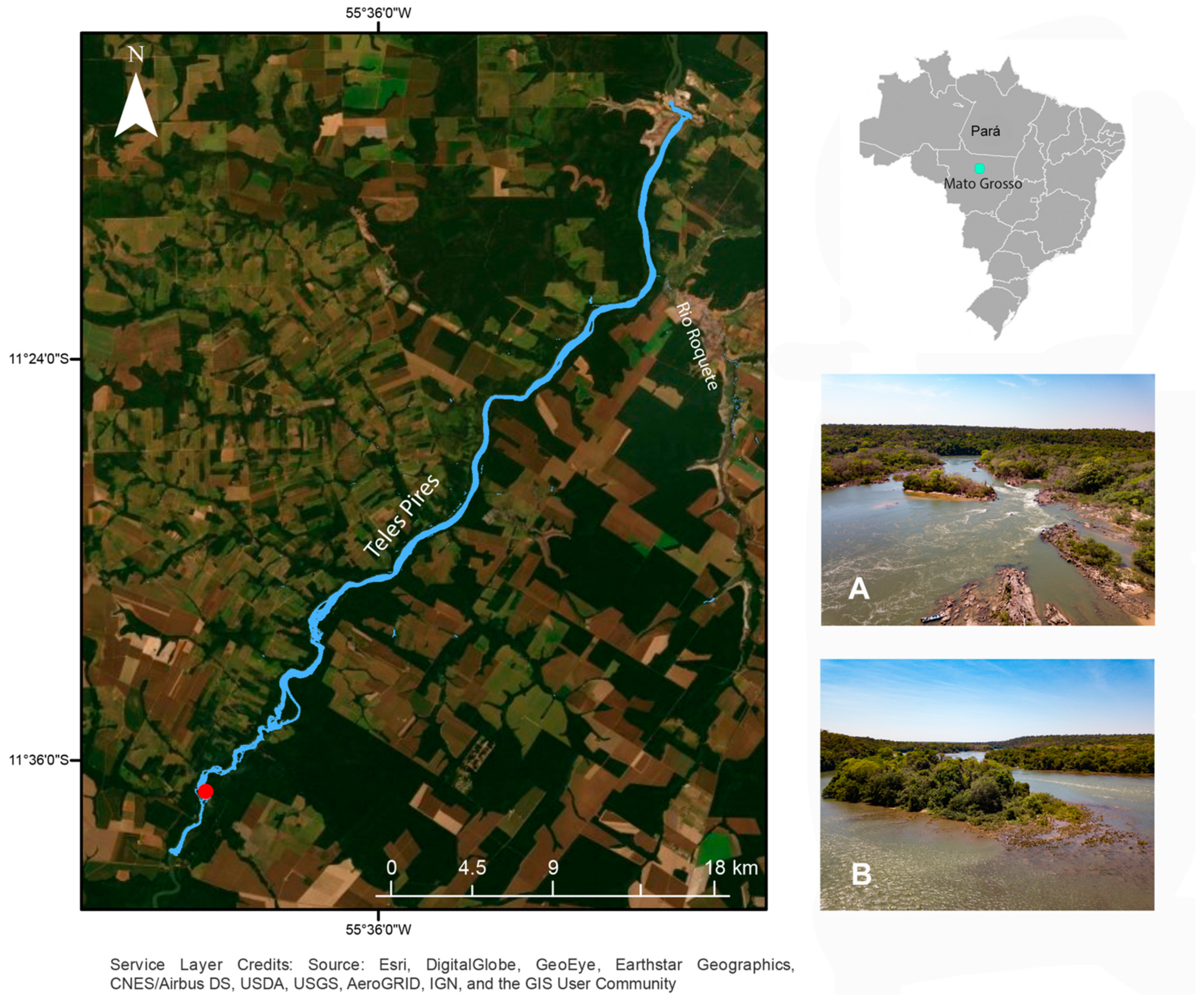
2.1. Study Area

The Teles Pires river forms the major eastern branch of the Tapajós river basin and is also the administrative border between the states of Mato Grosso and Pará. The most recent hydropower plant in the Teles Pires river complex, HPP Sinop (HPPS), is in the state of Mato Grosso, 70 km north of Sinop, serving the municipalities of Cláudia, Itaúba, Ipiranga do Norte, Sinop, and Sorriso. The HPPS is in the middle-upper portion of the Teles Pires river drainage within the Arc of Deforestation [51] where the landscape consists of large patches of deforestation mainly due to large scale commercial agricultural activities and was formerly referred to as the epicenter of deforestation in Brazil [52] (Figure 2). The HPPS began operations in September 2019. Its reservoir had a planned impoundment of 342 km² with an installed capacity of 401.88 MW. The actual area flooded by the Teles Pires following operationalization of the HPPS was considered as the study area for the satellite imagery analysis.

At a smaller scale, for UAS SfM-MVS photogrammetry, two sites on the Teles Pires were chosen: the fast-flowing rapids of the Corredeira do Suplício and the shallow, high flow, sand, and rubble zone on the upstream (north) side of Ilha do Lair (Figure 2). At the Corredeira do Suplício prior to inundation, white water rapids dropped in elevation by ~1 m and the Teles Pires is also narrower (~15 m wide) than elsewhere along the main channel. The substrate is composed of sand, stone, and large boulders. Due to the intense flow, only macrophytes of the Podostemaceae family that adhere directly on the rocks were present. In contrast, at Ilha do Lair, prior to the inundation there was a rapid current, but not as strong as at Corredeira do Suplício. This sector of the river is both wider (~150 m wide) and shallower than elsewhere in the main channel. Several species of macrophytes were present in a substrate composed of sand, stone, and small boulders. These two sites are part of the largest continuous stretch of rapids in the sector flooded by the HPPS reservoir. Prior to inundation the main channel had a pH ranging from 5.1–7.7, and average temperature of 24.5–29.3 °C.

In addition to the overall impact of the lentic zone on the landscape, changes to the biodiverse small creek tributaries during and after inundation were also examined from satellite imagery. These small tributaries, often only 1–3 m wide, flow into the Teles Pires river from the surrounding valleys and are especially vulnerable to change. They are found within riparian zones where the riverbanks retain a thin band of trees and palms. Water in these creeks was usually clear and fast-flowing (Figure 3). The streams in the region have acidic waters, with an average pH of 4–5.4, average temperature of 22.8–24.6 °C and mean conductivity of 7.52 ± 2.8 μS/cm (5.36–15.44 μS/cm).

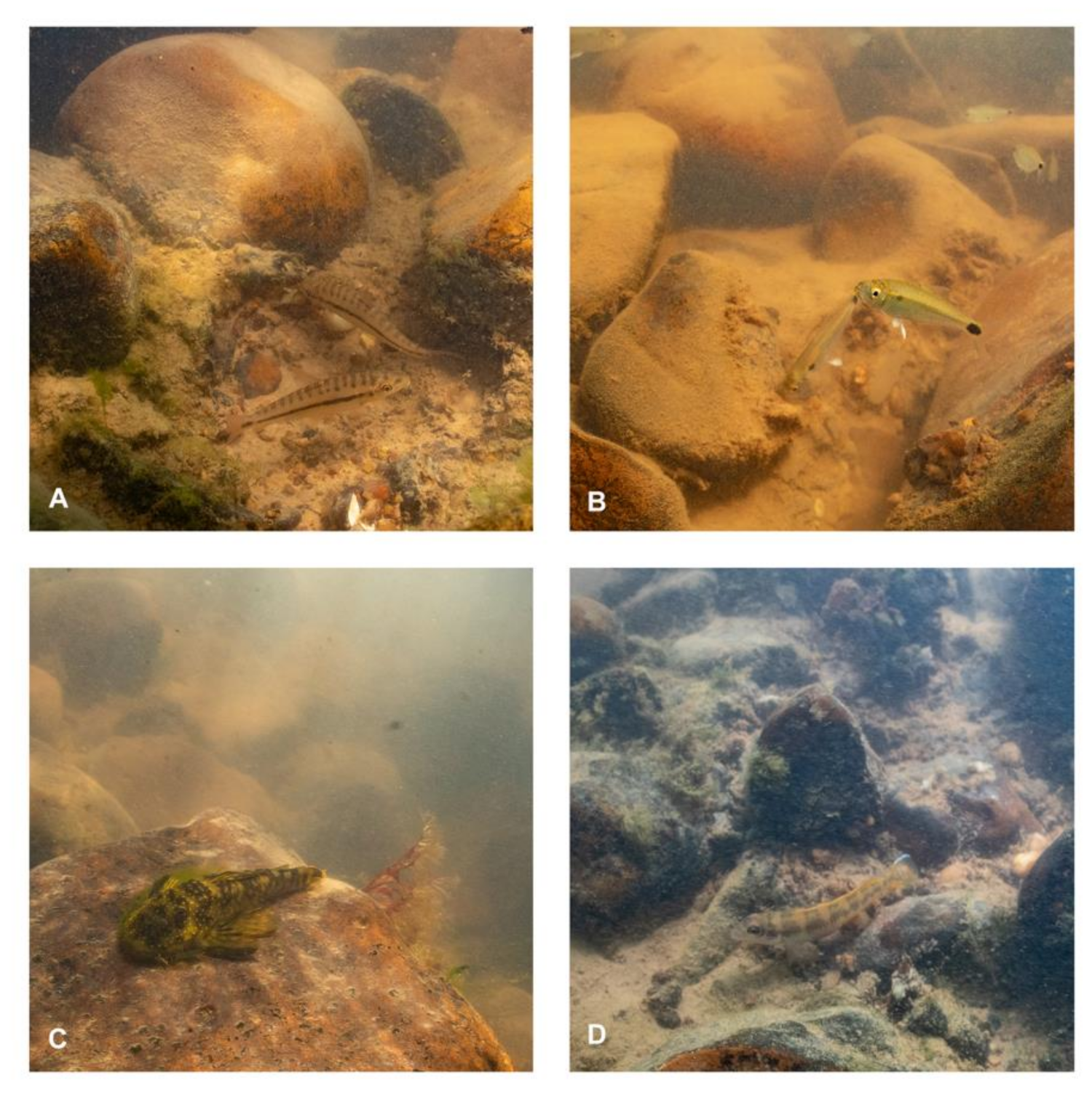
2.2. Aquatic Biodiversity

The annual migrations of the keystone species of the Amazon consist of millions of large fishes swimming up the various tributaries such as the Teles Pires [54]. The migrating fishes include well known giant catfishes such as Brachyplatystoma spp., Pseudoplatytstoma spp. and Phractocephalus hemioliopterus as well as many other fishes such as Hydro-lycus spp., Prochilodus spp., and Leporinus spp. Within the impact zone of the HPPS, Prochilodus nigricans (curimba), Brycon falcatus (matrinxã), Zungaro zungaro (jaú) and Pseudoplatystoma punctifer (pintado) also have reproductive migrations and are of interest as commercial species for fishermen in the region.

The upper middle Teles Pires river where the HPPS was constructed is one of the most biodiverse sectors of the river for fish. Rapids in the main channel are home to distinct rheophilic fauna and flora with adaptations for the extreme environment [55]. Species of Loricariidae (e.g., Peckoltia aff. cavatica, Scobinancistrus pariolispos), Anostomidae (e.g., Leporinus vanzoi, Sartor cf. elongatus), Serrasalmidae (e.g., Tometes sp. “Teles Pires”), Gymnotiformes (e.g., Sternacorhynchus aff. mormyrus, Archolaemus luciae), and Characiformes (e.g., Brycon falcatus, Bryconexodon trombetasi) were known to occur in the rapids at Corredeira do Suplício prior to inundation. Fishes highly adapted to the sectors with the strongest current and dense masses of Podostomaceae occur in the whitewater zone of the rapids. Highly specialized macroinvertebrate predators such as the Teleocichla sp. (Figure 4) and the rheophile catfish Pseudoancistrus kayabi (Figure 4) were commonly found at Ilha do Lair prior to inundation.

The fish communities in the streams are vastly different from the main river, with the predominantly smaller species that require both highly oxygenated fast flowing water and the three-dimensionally complex, silt free substrate for cover and feeding. Small characins such as Moenkhausia phaenota, Hyphessobrycon heliacus, and others were found in the creeks alongside small catfishes such as Corydoras apiaka, Curculonichthys luteofrenatus (Figure 3), Hisonotus chromodontus, and Centromochlus meridionalis. Prior to inundation, during the rainy season the flooding of the lower course of the creeks allowed species such as Brycon falcatus (a commercially important migratory species whose population is declining in this region) to travel upstream to the headwaters to breed [56]. Among the frugivorous fishes in the region, B. falcatus consumes the greatest abundance of fruits, and even young individuals can act as seed dispersers [57].

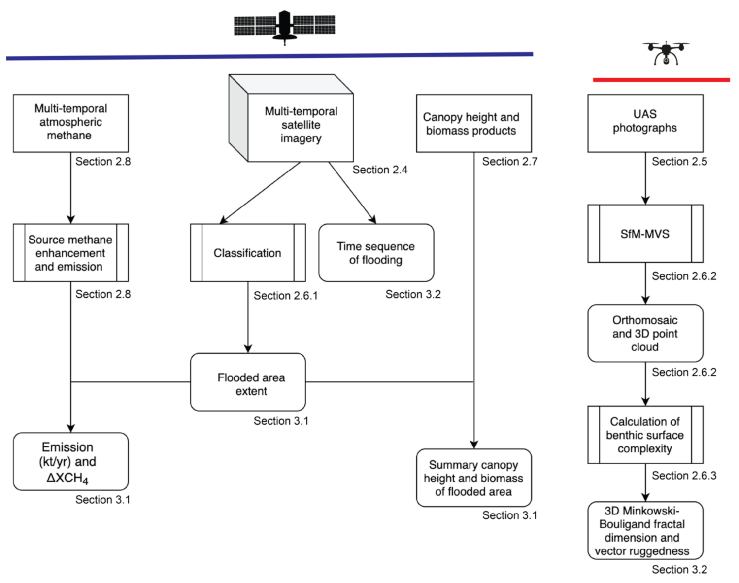
2.3. Overview of Data and Analysis

We present an overview of the datasets and analyses in Figure 5. Spaceborne (i.e., satellite) imagery and UAS-based photographs are employed at different scales to investigate the ecosystems impacted by the HPPS reservoir. Publicly available products describing vegetation characteristics (e.g., canopy height and biomass) as well as observations of atmospheric methane are used as ancillary data products to complement our analyses.

2.4. Satellite Imagery

RapidEye and PlanetScope (PS) satellite imagery were used for the classifications from both the low (dry season) and high water (end of the rainy season) periods (

Table 1. Satellite imagery used in the classifications.

Season	Dates	Constellation	No. Scenes
Low water, Pre-dam	May 31 and July 11, 2014	RapidEye	13
High water, Pre-dam	February 9, 2018	Dove PS	8
Low water, Post-dam	July 5, 7 and 8, 2020	Dove PS	24
High water, Post-dam	January 11, 15, 31, February 13, 14, 17, 2020	Dove PS	25

). The RapidEye constellation is comprised of five multispectral satellites which acquire five bands from blue to near infrared wavelengths [58]. The orthorectified, atmospherically corrected imagery used here has a pixel size of 5 m. The PlanetScope constellation consists of more than 130 triple-CubeSats (i.e., miniature satellites) with new satellites launched into orbit every 3–4 months [59]. The Dove PS satellites within that constellation acquire four-band multispectral imagery from blue to near infrared wavelengths. Analytic surface reflectance Dove PS images orthorectified to a 3 m pixel size were used [60]. All imagery was downloaded from Planet Explorer (https://www.planet.com/explorer, accessed on 29 May 2021) and mosaicked in ENVI 5.5 (L3Harris Geospatial, Melbourne, FL) prior to analysis (Figure 6).

In addition, monthly cloud free basemap mosaics generated from the PlanetScope constellation for the period of December 2018 to February 2020 were downloaded for a 57.6 km² tile centered on the confluence of the Teles Pires river and the Rio Roquete creek to illustrate the construction phase and subsequent seasonal change in flooding extent of one of the main small creek tributaries.

2.5. UAS Photograph Acquisition

Aerial photographs were acquired for the case study sites (Figure 2) by UAS. For Corredeira do Suplício, a DJI Inspire 2 quadcopter with an X5S camera (M4/3 sensor, 20.8 MP sensor resolution, 5280 × 3956 px image size, 3.3 µm pixel size) and a DJI MFT 15 mm f/1.7 ASPH lens was used to acquire 549 photographs in jpeg format on 4 September 2018 from an altitude of 60 m AGL. For the flight plan, a double grid pattern was used with 85% front and side overlaps. The flight path and camera triggering were controlled by the DJI Ground Station Pro iOS software. For Ilha do Lair, a DJI Mavic 2 Pro quadcopter with an integrated Hasselblad L1D-2C camera (1” sensor, 20 MP sensor resolution, 5472 × 3648 px image size, 2.35 µm pixel size) was used on 5 September 2018 to acquire 348 photographs in jpeg format (double grid pattern with 85% front and side overlaps) from 26 m AGL. The flight path and camera triggering were also controlled by the DJI Ground Station Pro iOS software. All photographs included the geolocation and altitude in the EXIF data.

Landscape models from UAS without real-time kinetic (RTK) or post processing kinetic (PPK) geotags of the photographs result in larger absolute positional errors of the models in real-world projected coordinates [24]. The within model accuracy of distances and volumes nevertheless remains high. Similar to [29], ground control points were not possible to acquire on site. The expected absolute positional accuracy in real-world coordinates of SfM-MVS models generated without ground control points of ~1 m error for the Inspire 2 and 2–3 m error for the Mavic 2 Pro [24] were considered adequate for the goals of this study.

2.6. Analysis

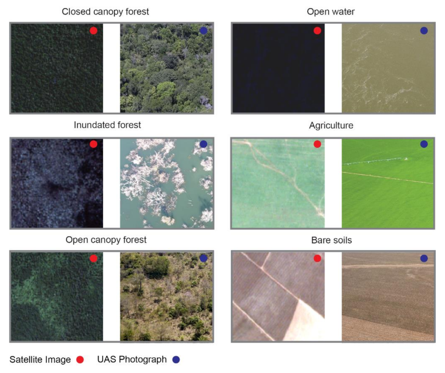
2.6.1. Satellite Image Classification

The satellite image mosaics from the four time periods (Table 1) were classified with eCognition Developer 9.4 (Trimble Geospatial, Sunnyvale, CA, USA) using a Geographic Object Based Image Analysis (GEOBIA) approach. GEOBIA classification is often more effective and efficient for imagery with high spatial detail and low spectral resolution [61,62] than pixel-based classification. It aims to replicate human interpretation of imagery by exploiting patterns, texture, and recognition of objects [63,64]. The four mosaics were first segmented with the multiresolution segmentation algorithm using the following parameters: scale = 50, shape = 0.1 and compactness = 0.5. Training samples of objects representing water, closed canopy forest, crops, soil, open canopy forest, inundated forest, and other throughout the study area were manually selected (Figure 7). The “other” class included, clouds, cloud shadows, and built-up areas. We included object level mean and standard deviation values of brightness (i.e., average of the means of the bands), maximum difference (i.e., maximum difference between bands), and the reflectance from each band in the nearest neighbor feature space for training data for a nearest neighbor classification.

The resulting individual classes were simplified to water (including open water and inundated forest), soils and agriculture, and forest (including closed and open canopy forest) in ArcMap 10.7 (ESRI, Redlands, CA, USA). The polygon layers were inspected through an overlay with the corresponding mosaic and erroneous class labels were corrected manually (e.g., dark shadows along the boundary between forest and soil classes). For the few areas where small clouds obstructed the classification of the reservoir margins of the high-water mosaic (Jan–Feb 2020), the polygon vertices were edited to trace the shoreline of the reservoir without cloud cover. The final edited polygon layers from each mosaic were dissolved to classifications representing water, forest, and soil/agriculture.

Three hundred sixty-nine random points (distance ≥ 30 m) were generated within the footprint of the high-water reservoir extent in ArcMap. The associated land cover class was manually interpreted for each point from the low water, pre-inundation satellite image mosaic (2014), and used to assess the accuracy of the classifications of the land cover within the footprint of the reservoir.

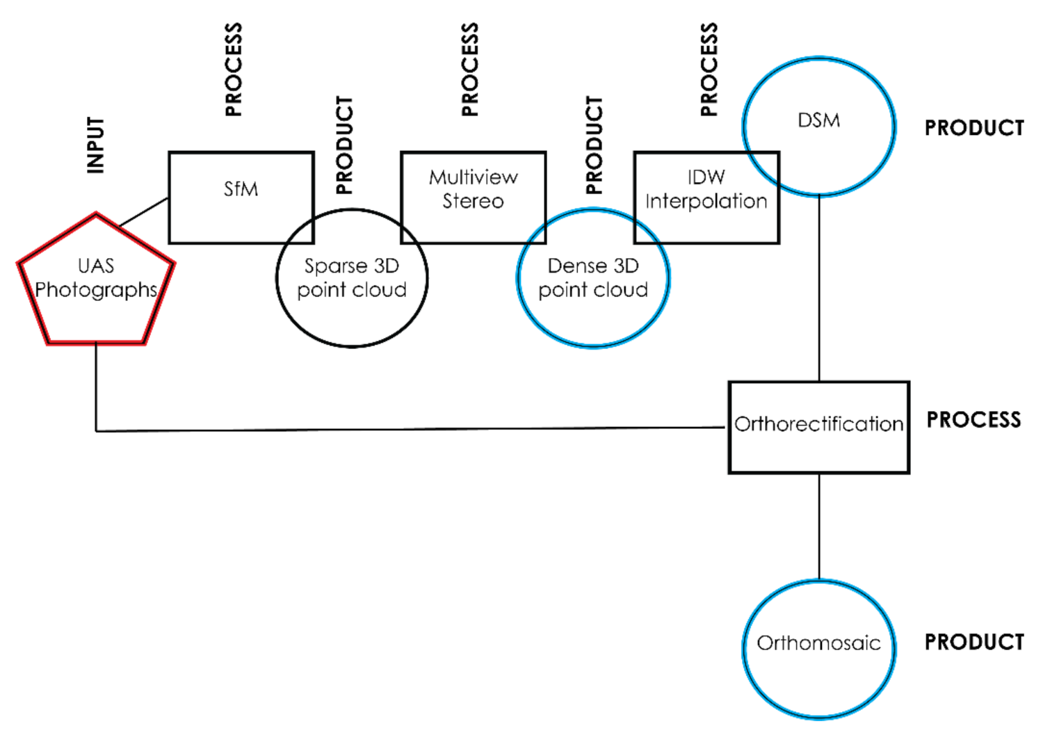
2.6.2. Structure from Motion Multi-View Stereo Photogrammetry (SfM-MVS)

We used Pix4D Mapper v4.6.4 (Pix4D, Prilly, Switzerland) for the SfM-MVS workflow (Figure 8). The inputs into the workflow were the jpg photographs acquired by UAS. The final products, namely the dense 3D point cloud, the orthomosaic and the digital surface models (DSM) are the result of a multi-step process. In the first step, Pix4D optimizes both internal (e.g., focal length) and external (e.g., orientation) camera parameters and carries out an automatic triangulation and bundle block adjustment [65]. Keypoints, representing points in each photograph with a unique and identifiable texture, are located. These keypoints are then matched between neighbor photographs. The sparse point cloud (output of this first step) is generated through a modified scale-invariant feature transform (SIFT) algorithm [66,67]. In step two, the point cloud is densified with a multi-view stereo (MVS) photogrammetry algorithm [68]. The output of this step, the dense point cloud, is one of final products used for further analysis. In step 3, the dense point cloud is interpolated with an inverse distance weighting (IDW) algorithm to generate the DSM in raster format. The input photographs and the DSM are used to generate an orthomosaic without perspective distortion. The DSM and orthomosaics are the other two final products used and discussed in this study.

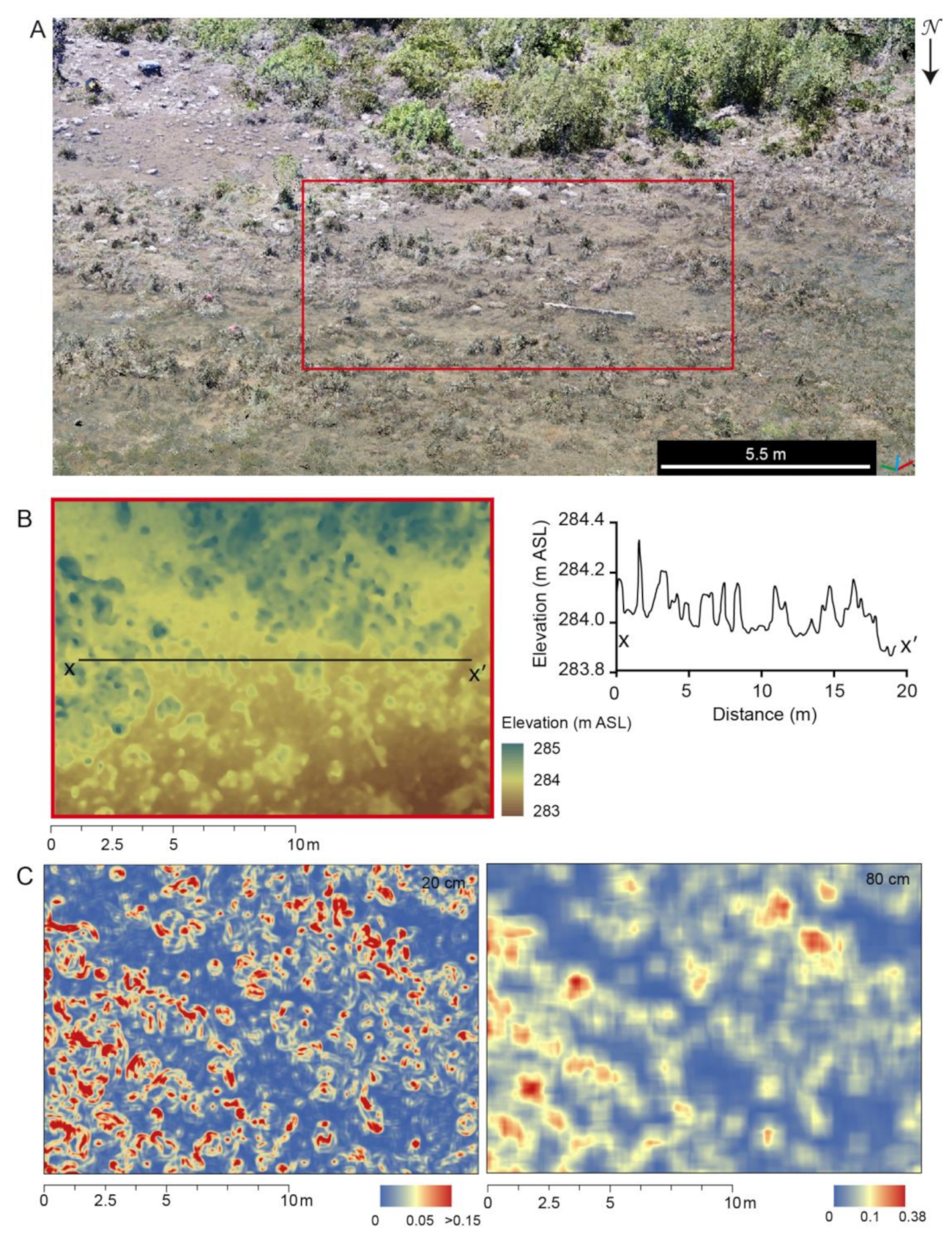
2.6.3. SfM-MVS Products

Measures of benthic surface complexity computed from SfM-MVS models are robust and repeatable metrics. Aquatic biodiversity has been shown to be strongly related to habitat structural complexity (e.g., [69,70]). Among the various ways in which complexity is defined, here we refer to it as the heterogeneity in the arrangement of substrate types [71]. As examples of complexity metrics that can be readily determined from SfM-MVS products, we computed two spatial properties of the Ilha do Lair DSM, vector ruggedness and the 3D Mindowski–Bouligand fractal dimension.

The vector ruggedness was calculated at window sizes of 20 and 80 cm for a subset of the DSM with the Benthic Terrain Modeler toolbox in ArcMap [72]. This measure quantifies ruggedness as the variation in the 3D orientation of the surface incorporating both slope and aspect heterogeneity [73]. Unlike other measures that are correlated with slope (e.g., terrain ruggedness index), this metric quantifies local variations in the terrain independently.

For the same subset area of the Ilha do Lair data, the dense point cloud was converted to a triangular mesh in CloudCompare Stereo v.2.11.3 (https://www.danielgm.net/cc/, accessed on 29 May 2021) at the original GSD and scales of 20 and 80 cm. These meshes were used to compute the 3D Mindowski–Bouligand fractal dimension of the substrate [74,75]. The value of the fractal dimension, D, varies from 0–3 where higher values indicate a more complex surface.

With ecological knowledge of the fish fauna, products quantifying the three dimensional characteristics of the substrate (e.g., elevation, slope, vector ruggedness, etc.), can further be used to classify the habitat according to the preferences of different fish or plant species. For example, rheophile cichlid and Loricaridae species require caves of varied sizes for breeding, and slope and surface texture influence the biocover and microinvertebrate fauna that many rheophile fishes feed on [29].

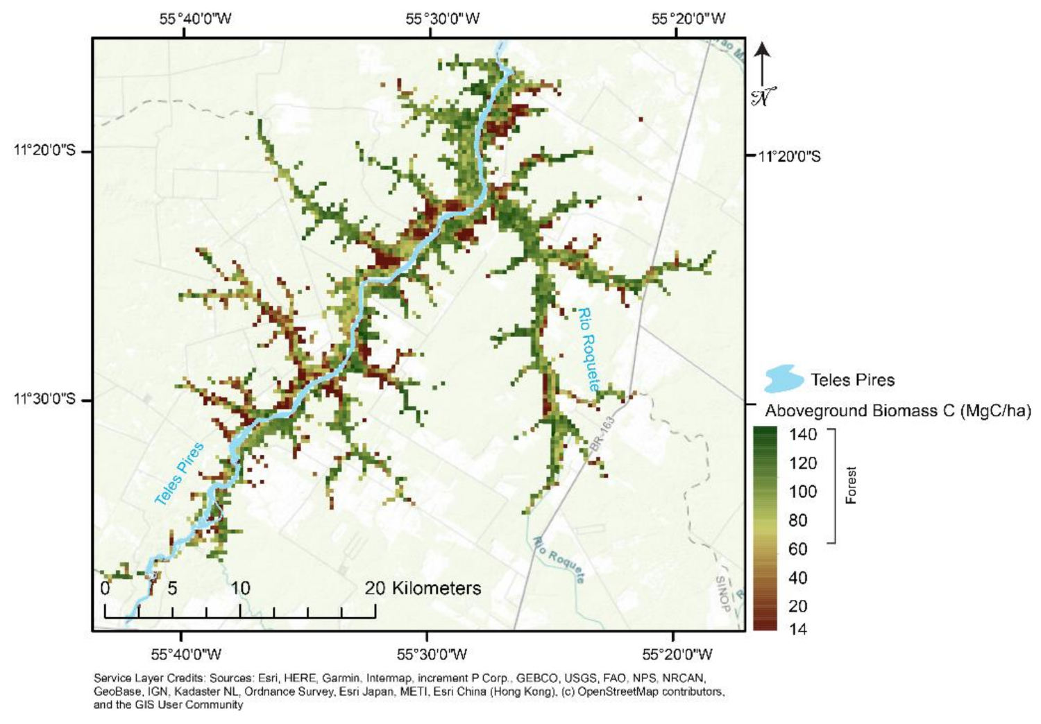
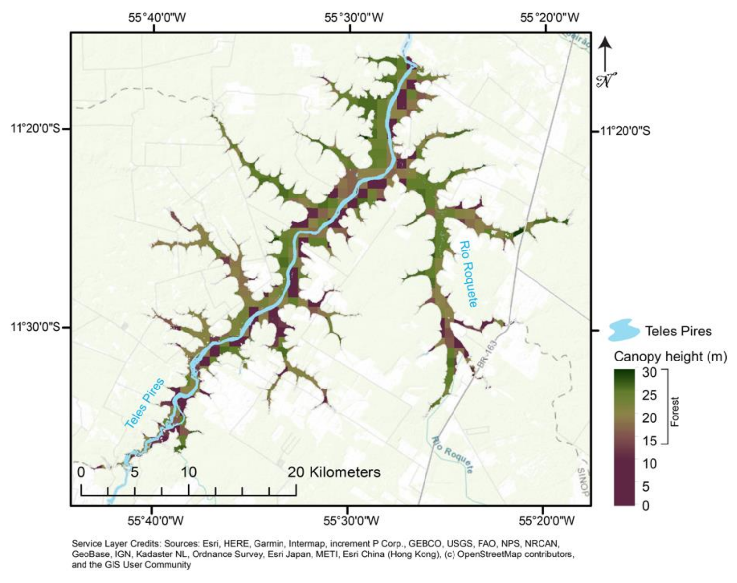
2.7. Spaceborne LiDAR, Terrestrial Carbon Biomass

From the Google Earth Engine repository, we downloaded global tree canopy height data (circa 2005) produced from the Geoscience Laser Altimeter System (GLAS) spaceborne LiDAR aboard ICESat (Ice, Cloud, and land Elevation Satellite) [76] for the lentic zone. GLAS transmits laser pulses at 1024 nm with footprints of ~65 m diameter and records the reflected waveform. The data were available at a spatial resolution of 30 arc seconds.

Harmonized above and below-ground terrestrial carbon (MgC/ha) estimates (circa 2010) [77,78] were downloaded from the Oak Ridge National Laboratory Distributed Active Archive Center (ORNL DAAC). The aboveground C data represent a compilation of pre-existing, publicly available ecosystem data. For below-ground C, land cover specific root-to-shoot relationships had been used to generate maps for each of the input above-ground C maps prior to harmonization (300 m resolution) (see [77] for details). Both above and below ground biomass C stock densities are limited to living plant tissues. We summarized the above and below ground C for the pre-inundated forest area within high water reservoir boundaries.

2.8. Atmospheric Methane Concentration

Lastly, satellite-based measurements of the total column-averaged dry-air mole fraction of methane (XCH₄) for a 26,000 km² region surrounding the HPPS lentic zone from the TROPOspheric Monitoring Instrument (TROPOMI) onboard the Copernicus Sentinel-5 Precursor (S-5P) satellite were downloaded from the Google Earth Engine repository [79]. The data product represented the two-band retrieval utilizing the 2.3 µm methane absorption band and the 760 nm oxygen absorption band to determine methane abundance in the atmosphere at 7 × 7 km resolution [79,80]. Cloud-free data were available for the months of July and August, 2020. A 1,414km² convex hull was fit around the high-water season reservoir to which a 1 km buffer had been added. This area of interest was removed from the larger 26,000 km² region, the remainder considered as the regional background. For comparison, methane abundance was also extracted over a 17,500 km² area of intact protected forest in the Xingu National Park located 200 km to the east. We determined the source methane enhancement (ΔXCH₄) by subtracting the mean XCH₄ difference between the reservoir area of interest and the regional background. We estimated emission according to the mass balance method from [81]. The monthly average values of wind speed and surface pressure needed for the calculations were extracted from the ERA5-Land monthly averaged ECMWF climate reanalysis data [82].

2.9. Visualization

Improvements in personal computing as well as internet access becoming a near-ubiquitous aspect of daily life in many countries, also present the potential of scientific data sharing, visualization and collaboration through digital means. We illustrate straightforward examples of temporal and immersive visualization options for both the satellite imagery and SfM-MVS products. For dynamic visualization of land cover change around the HPPS we examined the newly launched Google Earth Timelapse. This option only requires access to a web browser and an internet connection. Cloud free satellite images can be viewed as a time lapse animation, qualitatively illustrating the changes on the surface of the Earth over a 36-year period (1984–2020).

We also explored the use of immersive virtual reality (VR) technology for visualization of satellite imagery and SfM-MVS products. Virtual reality is the combination of hardware and software to simulate an environment with the user experiencing a high ‘sense of being present’ in the VR representation [83]. VR experiences are immersive and can be a cost effective way to visualize scientific data. Gaining popularity in fields such as medicine [84], and ecology [85], among others, it is also beneficial for geospatial sciences [86]. We tested two readily available VR head mounted displays (HMD), the Oculus Quest 2 (Facebook Technologies LLC, Menlo Park, CA. USA) and a second generation Google Official 87002823-01 Cardboard viewer (Google, Mountain View, CA, USA).

The Oculus Quest 2 is a low-cost, consumer-grade standalone HMD with 6 GB RAM, an Android based operating system and internal storage. The lenses have a resolution of 1832 × 1920 pixels per eye and are capable of a refresh rate of 72–90 Hz. By connecting the HMD to a computer and initializing the Oculus Link software, the HMD can access additional software and data that require more computational power to run than is possible from the HMD alone. We accessed the satellite imagery archive on Google Earth VR for the HPPS study through this manner. We also illustrate the immersive nature of the SfM-MVS point clouds by interacting with them in the Oculus Quest 2 through the free VRifier software (accessed through Oculus Link). As a lower cost alternative compatible with the Google Cardboard viewer, we uploaded the SfM-MVS models to Sketchfab, a web based VR viewer (https://sketchfab.com, accessed on 29 May 2021). The web based VR viewer allows users to interact with content through their smartphone’s browser and a basic VR viewer.

3. Results

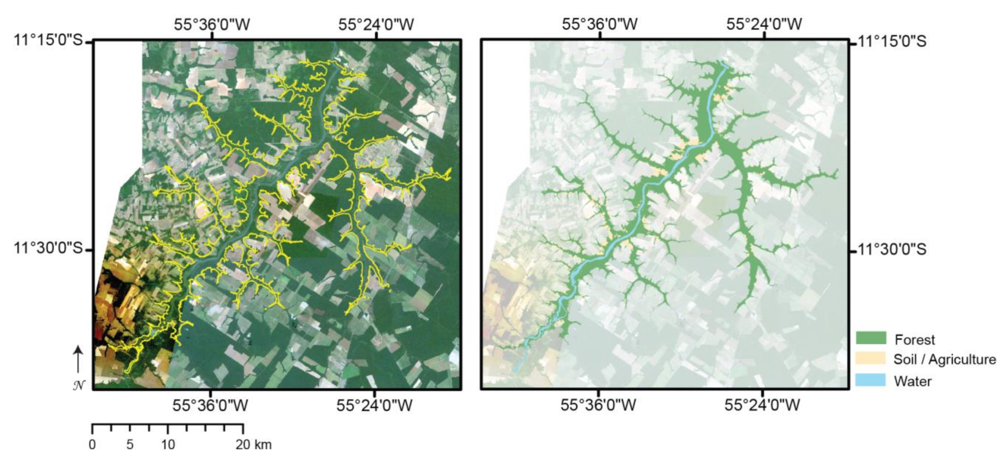
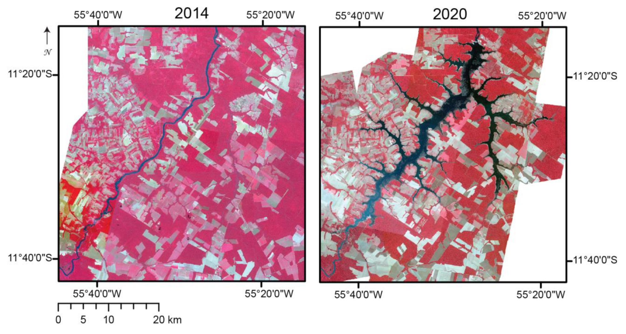
3.1. Land Cover Composition Prior to Flooding

The area of each land cover class flooded by the HPPS is shown in

Table 2. Land cover class areas within the lentic zone of the HPPS determined for low water (July) and high water (Jan-Feb) seasons from Dove PS imagery acquired in 2020 (Table 1).

Land Cover	Area (km2) Low Water	Area (km2) High Water
Water	19.79	19.91
Soil/Agriculture	25.62	38.10
Forest	163.04	177.07
Total	208.45	235.08

for both high water (i.e., end of rainy season, Jan-Feb) and low water (i.e., dry season, July) periods. The class with the greatest area impacted is forest (163.04 km² during low water and 177.07 km² during high water), followed by the soil and agriculture classes (25.62 km² and 38.10 km² respectively). The spatial distribution of the flooded classes in the landscape can be seen in Figure 9. Overall, for the year 2020, we found the flooded area in the low water season was 208.6 km² and 235.08 km² in the high water season. This represents 106.9–133.4 km² less than the 342 km² stated in the HPPS planning documents [87]. In the planning documents, the extent of the flooding was expected to extend south of the MT-220 highway, but in our analysis of the high spatial resolution imagery, we found the flooding did not extend past the bridge on the MT-220 crossing the Teles Pires (Figure 9).

As shown in

Table 3. Confusion matrix for the 2014 low water RapidEye classification.

	Forest Reference	Water Reference	Soil/Agriculture Reference	User’s Accuracy (%)
Forest classification	211	0	9	95.9
Water classification	1	54	0	98.2
Soil/Agriculture classification	6	0	88	93.6
Producer’s Accuracy (%)	96.8	100	90.7	OA = 95.7%

, the accuracy of the land cover classes pre-flooding within the lentic zone was high for each of the three classes (>90% user’s and producer’s accuracies) with an overall accuracy of 95.7%.

The canopy height estimates from GLAS indicate that within the lentic zone (high water season), the forest canopy ranged from 13–30 m tall (Figure 10). The majority of the tall trees were found along the banks of the small tributaries such as the Rio Roquete, and along the western banks of the Teles Pires river. Estimated aboveground biomass C (Figure 11), indicate an average of 91.0±31.0 Mg/ha for the forest within the lentic zone during the high-water season. Below ground biomass C for the same forest area was estimated at 22.3 ± 7.1 Mg/ha for a total of 113.3 ± 38.1 Mg/ha.

We found a small ΔXCH₄ for both July (2.65 ppb) and August (4.4 ppb) comparing the XCH₄ of the HPPS lentic zone to the regional background (

Table 4. Monthly average XCH₄ from TROPOMI.

Site	Month	XCH4 (ppb) (µ ± σ)
HPPS lentic zone	July	1852.5 ± 6.8
HPPS lentic zone	August	1856.3 ± 9.4
Background region	July	1849.8 ± 14.2
Background region	August	1851.9 ± 15.9
Xingu National Park	July	1807.5 ± 10.0
Xingu National Park	August	1809.9 ± 10.8

). A small difference was expected because the background consists of a large proportion of agriculture/soil (49.5% of the area [88]). It also includes six small municipalities and the city of Sinop. The difference in average XCH₄ is greater when comparing the HPPS lentic zone with the intact forest of the Xingu National Park (ΔXCH₄ = 45 ppb for July and 46.4 ppb for August). Gross estimates of CH₄ emission for the HPPS lentic zone indicate 48.5 kt/yr based on the ΔXCH₄ from July and 54.8 t/yr based on the ΔXCH₄ from August. A longer time sequence of cloud free TROPOMI observations would be needed to account for seasonal variation in ΔXCH₄ and a more accurate annual estimate.

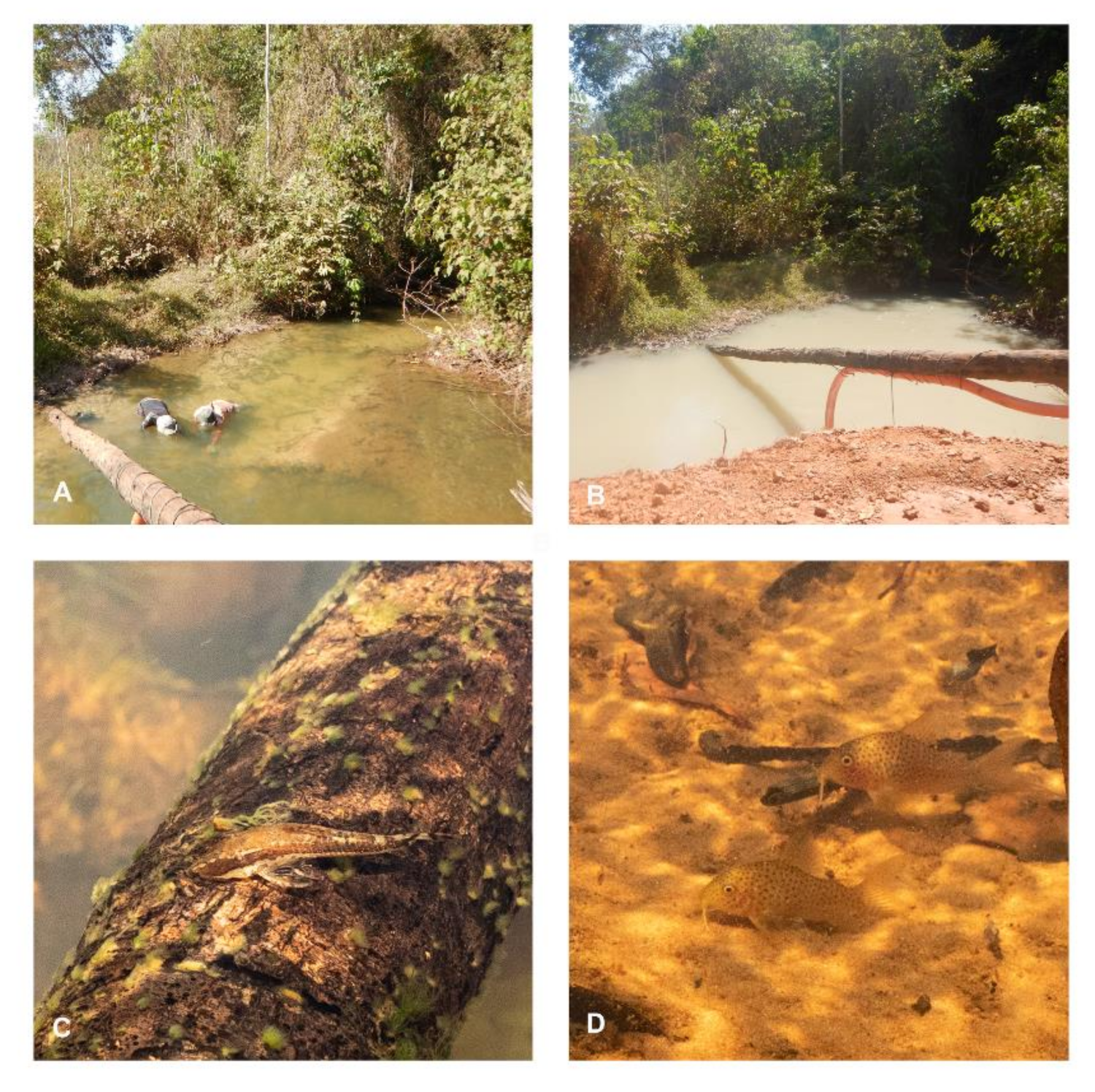
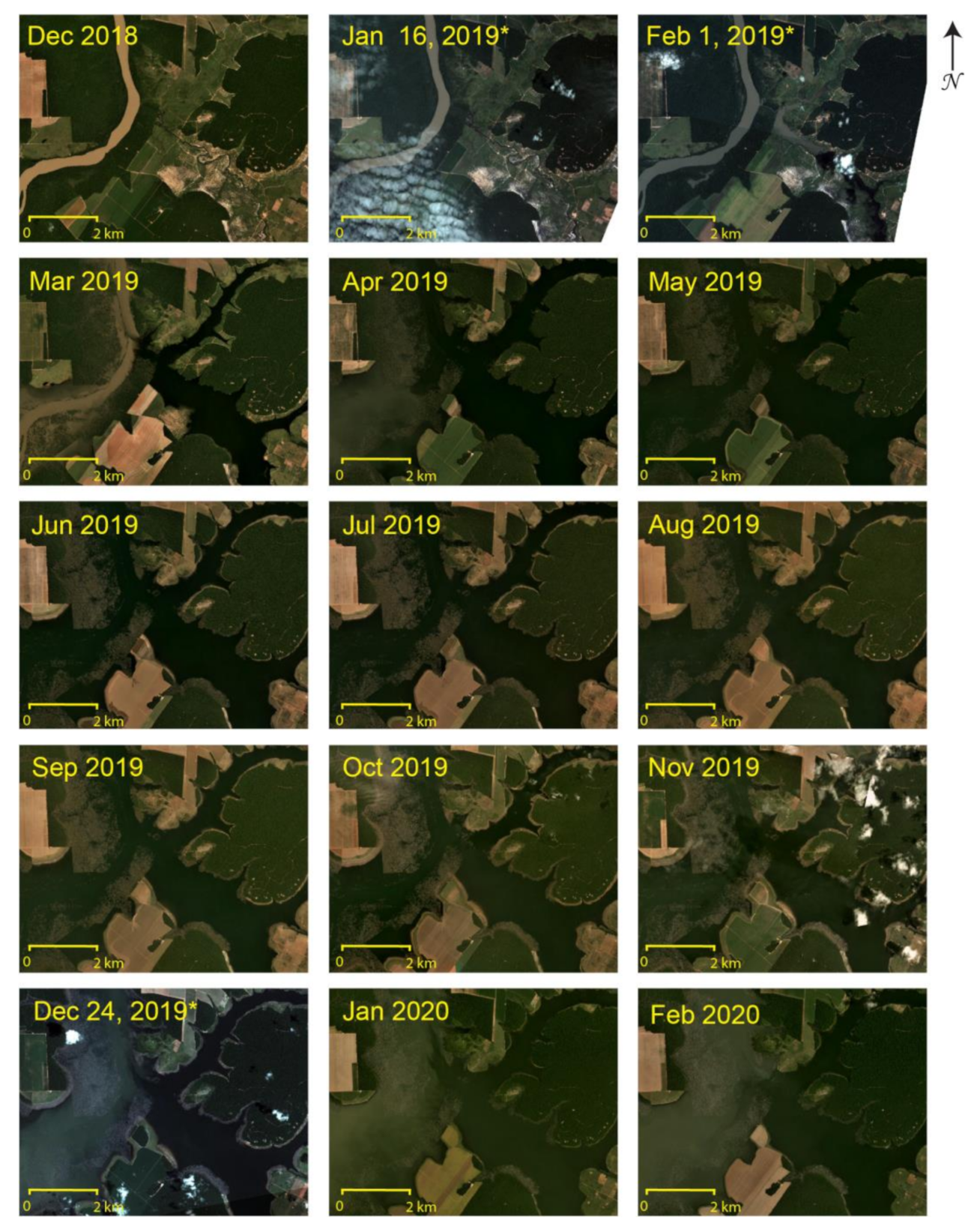
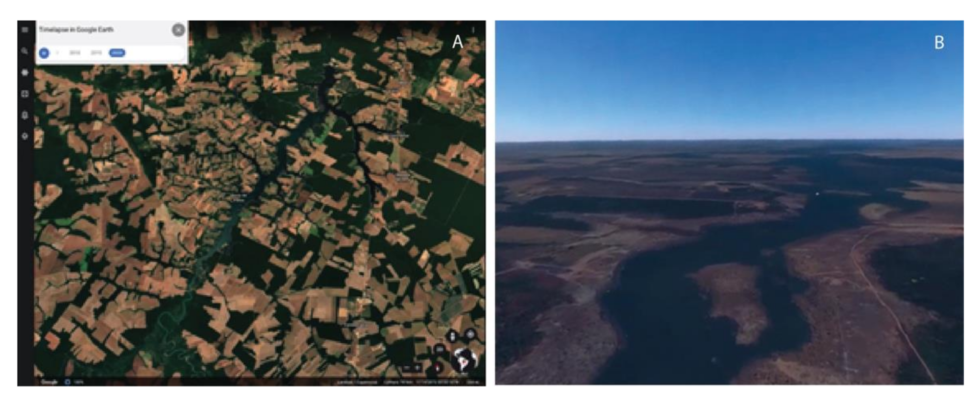
3.2. Flooding of Small Stream Tributaries

The daily revisit period of the Dove PS constellation allows for a dense time sequence view of the filling of the reservoir and the impact the filling had on the small creek tributaries. As an example, we illustrate the sequence for the confluence of the Rio Roquete creek and the Teles Pires river over the December 2018–February 2020 period (Figure 12). In December 2018, the original course of the narrow stream can be seen draining into the Teles Pires river. The forest has been cut along the banks of the stream in the area planned to be flooded by the HPPS reservoir. The same can be seen from the image acquired 16 January 2019, prior to the filling of the reservoir. From the image acquired 1 February 2019 one day after the filling began, the incursion of water from the silt laden Teles Pires (high water) into the creek can be seen, along with the stream having overflowed its usual banks. In March, not only has the flooded stream surface area increased considerably, covering nearly the entire expected range, but the main branch of the Teles Pires can also be seen flooding standing forest on the banks. In April 2019, the flooding of the Rio Roquete creek is complete, and the main branch of the Teles Pires has also widened to include flooding of forest and agricultural areas. There is a marked decrease in turbidity over the course of the low water season (June–August). The turbidity of the Teles Pires increases again in the high-water season (December 2019–February 2020). From February 2019 onwards, silt from construction, modification of the riverbanks to prevent flooding, and permanent inundation from the reservoir have permanently changed the habitats in the small stream tributaries.

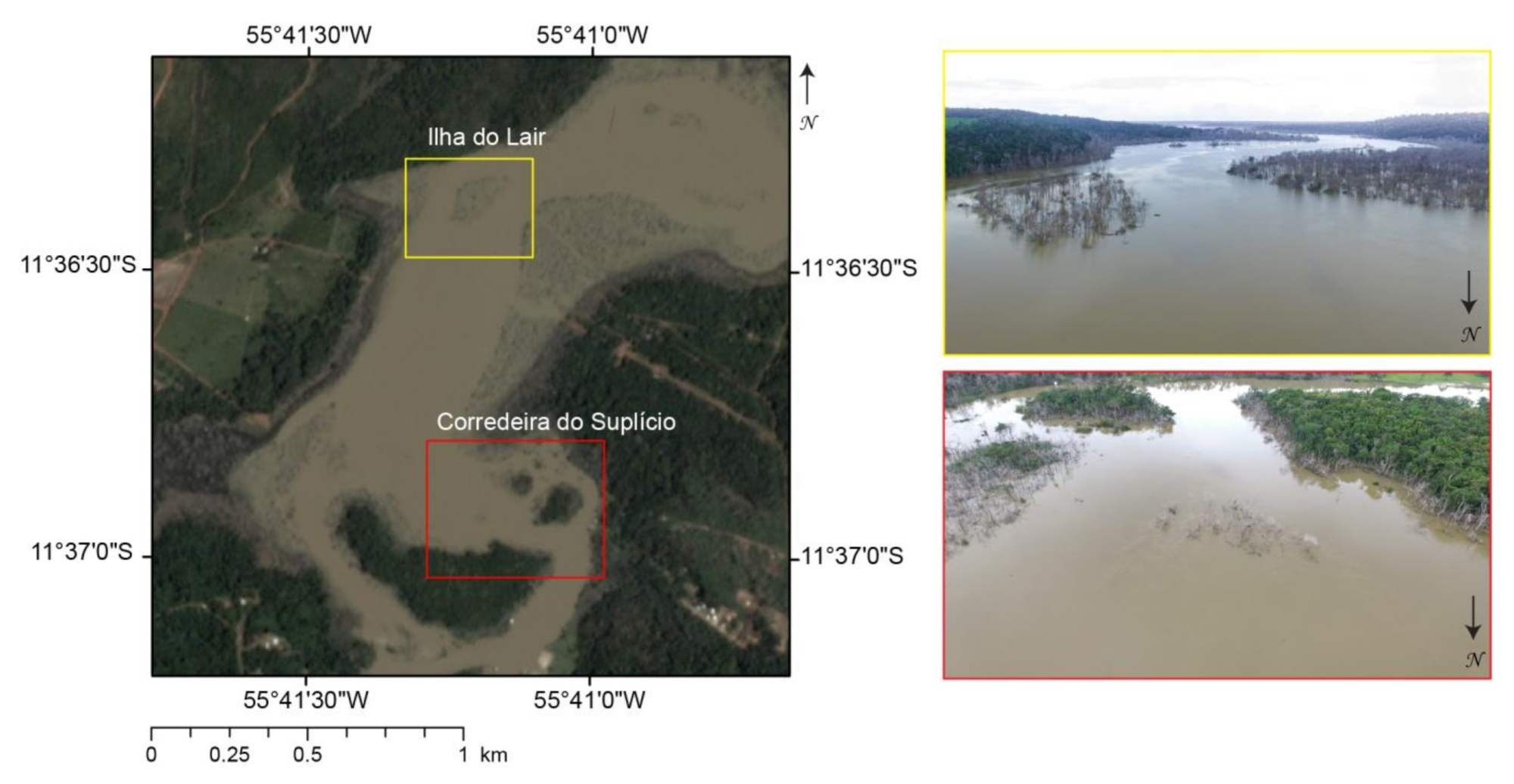
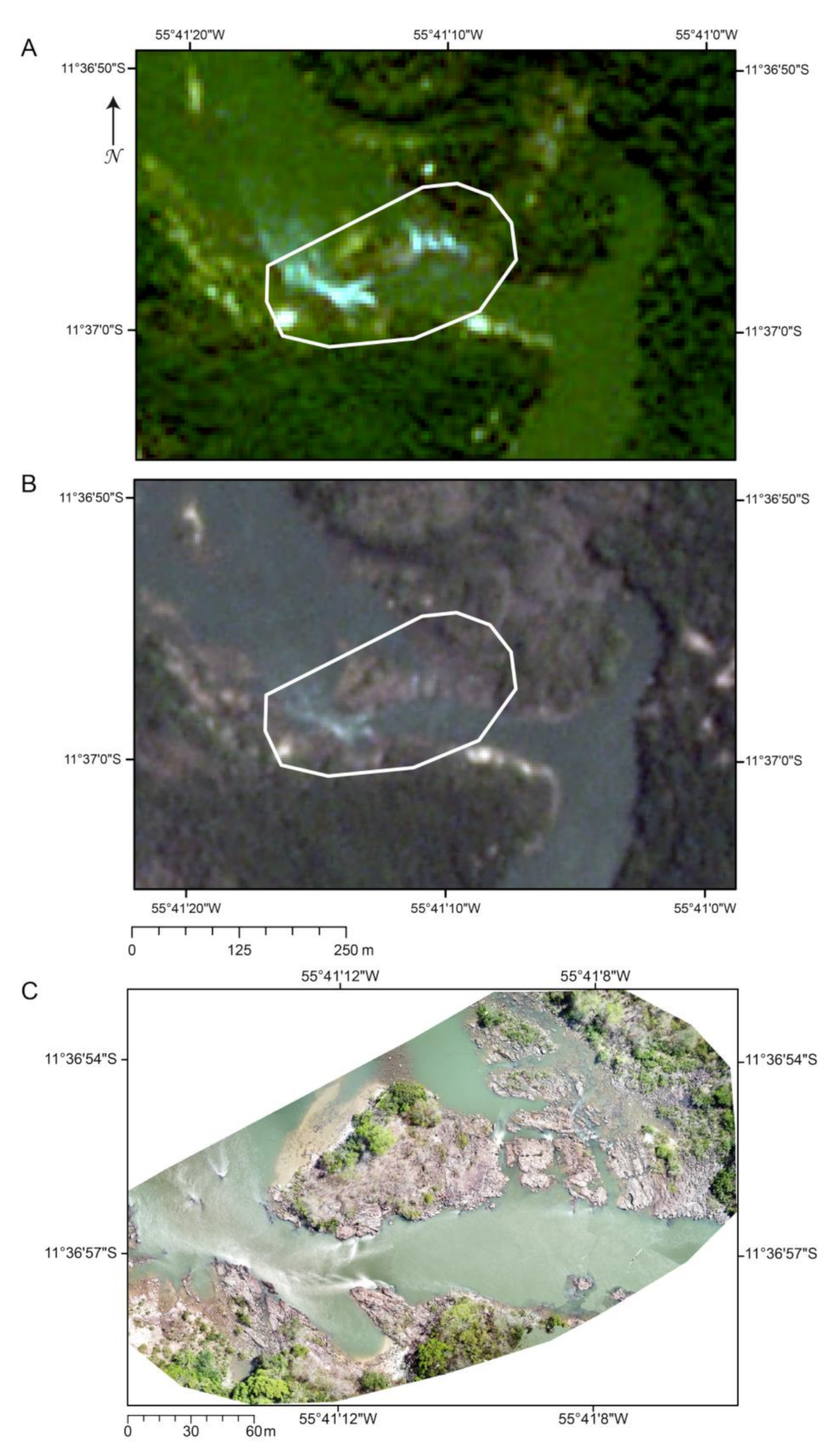
3.3. UAS Case Study Areas and SfM-MVS Products

In comparison to the conditions pre-flooding (Figure 2), both UAS case study areas have been substantially modified post-flooding (Figure 13). Both areas are within the lentic zone of the HPPS and now permanently covered by deeper and slow-moving water. Both the UAS photographs and Dove PS imagery acquired in February 2021 show the areas have been fully submerged in the slow-moving water. Only the tops of the trees on Ilha do Lair can be seen out of the water, while at Corredeira do Suplício the rapids are no longer present.

For Corredeira do Suplício, the final ground sampling distance (GSD) of the SfM-MVS products was 2 cm. Pix4D located a median of 49,773 keypoints per photograph and a median of 7745.8 matches between neighbor photographs. The final 3D point cloud has an average point density of 584.6 pts/m². For Ilha do Lair, the GSD of the SfM-MVS products was 0.9 cm. Pix4D located a median of 51,394 keypoints per photograph and a median of 15,788.2 matches between neighbor photographs. The density of the final 3D point cloud is 7885.6 pts/m².

A closer look at the Corredeira do Suplício illustrates the difference in scales between the high spatial resolution satellite imagery (3–5 m pixel sizes) (Figure 14a,b) and the UAS orthomosaic (Figure 14c), one of final products from the SfM-MVS workflow (Figure 8).

At Ilha do Lair, the DSM shows the shallow water zone on the upstream side of the island. This site with high flow was populated by juveniles of many species, as well as smaller species foraging in the dense masses of plants. With the permanent inundation these types of habitats are covered in sediment and no longer available for the rheophile species. Figure 15 shows the Ilha do Lair 3D point cloud, DSM and vector ruggedness at different sizes pre-inundation.

The fractal dimension of the Ilha do Lair triangular mesh at the original GSD of 0.9 cm was 1.99. The value of D decreased considerably to 1.09 at a resampled resolution of 20 cm and to 1.08 at a resampled resolution of 80 cm. This indicates that the greatest complexity in this habitat was found at smaller spatial scales, however, once the fine scale complexity is removed there is minimal difference between the complexities at the coarser scales. For fish such as the Teleocichla sp. (Figure 4) which have a small body size (~12 cm TL), the fine scale complexity is important because they rely on caves dug under these rocks for breeding, complex bottom structure for cover, and on microinvertebrates living in the dense mass of biocover (e.g., algae) growing on the rocks.

3.4. Data Visualization

The most accessible and straightforward visualization of the satellite imagery was through the Google Earth Timelapse (Figure 16a). Through the animation it is possible to see the extensive land cover change from forest to agricultural activities beginning in earnest around 2000. The lentic zone is also visible as of 2019. A static 3D representation of recent (post flooding) satellite imagery of the HPPS lentic zone can also be accessed through Google Earth VR via the Oculus Quest 2 headset (Figure 16b). In this VR environment, for the area encompassing the HPPS lentic zone, recent (post flooding) high resolution satellite imagery has been draped over a global DEM to provide a 3D view of the topography. Similar to the ubiquitous personal computer version of Google Earth, in this VR version, the user can navigate through the landscape. The flooded forest and extensive agriculture surrounding the reservoir is readily apparent in this viewing experience. Because it requires an HMD connected to a computer, the set-up is more complicated, and while there is no temporal change in the imagery, there is a greater sense of immersion into the data than from conventional viewing on a monitor.

Virtual reality HMD and Google Cardboard compatible versions of the SfM-MVS 3D point clouds can be viewed at https://skfb.ly/onFFS, accessed on 29 May 2021 (Corredeira do Suplício) and https://skfb.ly/onEEp, accessed on 29 May 2021 (Ilha do Lair). The Google Cardboard viewers are specific to the screen size of the smartphone, the version used here was compatible with phones with screens up to 6” in size. When viewed on and iPhone 11 Pro, the stereoscopic effect was clear with both models. Basic teleportation within the model was also possible. The most immersive VR experience with the datasets was when they were accessed locally with the Oculus Quest 2 through VRifier (Figure 17). While it is not yet possible to carry out quantitative analyses within the VR platform, new developments in the software capabilities are expected to provide such features.

4. Discussion

The Amazon Basin, roughly two-thirds of which is in Brazil, is the focus of a massive surge in hydroelectric dam construction, with plans that would eventually convert almost all Amazon tributaries into chains of reservoirs [49]. Greenhouse gas emissions from the lentic zones of hydropower dams have been intensively studied, with a focus on the high CH₄ emissions [42,89,90,91]. Due to the increased global warming effect of CH₄ in the atmosphere, the proclaimed “green” energy generation from hydroelectricity has further been questioned [92]. For the HPPS, the estimate of yearly CH₄ emission from TROPOMI data (48–54 kt/yr) is within the range of reservoir emissions measured in eutrophic systems [90]. As more observations become available, the seasonal variability should be considered for a more accurate yearly estimate. For comparison, the CH₄ emission from biomass burning in the legal Amazon (1992–1993) ranged from <100 kt/yr (Amazonas, Roraima) to 1300 kt/yr (Mato Grosso) [93]. The greatest contributing factor to the amount of CH₄ emission from a reservoir is the amount of flooded vegetation that was not cleared prior to inundation, rather than reservoir age or location [90]. In the case of the HPPS lentic zone, flooded forest was the largest land cover class within the reservoir boundaries accounting for 75–78% (high and low water seasons, respectively). Canopy height data from GLAS indicated that the forest in the lentic zone was of reasonably tall stature (up to 30 m) (Figure 10) and biomass estimates indicated a combined AGB and BGB of 113.3 ± 38.1 Mg/ha (Figure 11).

Almeida et al. [43] estimate the 20- and 100-year C intensities of HPPS as 1052.6 and 358.3 kg CO₂ eq MWh⁻¹, respectively. The C intensity is the CO₂-equivalent emissions produced per unit electricity generated [43]. The estimate for HPPS is considerably higher than the 20- and 100-year C intensities of the Belo Monte dam complex on the Xingu River, one of the largest run-of-the-river dams in the world [94] (62.2 and 37.9 kg CO₂ eq MWh⁻¹) [43], but less than those of Balbina dam on the Uatumã River (12,004.5 and 3901.3 kg CO₂ eq MWh⁻¹ [43]. Under different global warming scenarios, [95] estimate that HPPS’s 100 year C intensity could exceed 2000 kg CO₂ eq MWh⁻¹. For comparison, the C intensity of bituminous coal thermal plants is 792 kg CO₂ eq MWh⁻¹ and 348 kg CO₂ eq MWh⁻¹ for combined cycle gas thermal plants [92]. One hundred years after inundation, HPPS is estimated to approximate the C intensity of a natural gas thermal plant.

While other studies have used pre-existing land cover datasets (e.g., [96]), to infer the impact of hydroelectric reservoirs on the landscape, there is substantial variability in the amount of forest and non-forest classes in both national and global datasets [5]. Hence, relying on such global datasets to assess the impact of hydroelectric reservoirs may not be adequate. In our study we generated a high spatial resolution classification of the land cover within the HPPS lentic zone leading to more precise estimates of inundated classes. This is of particular importance for the Riparian vegetation along the small creek tributaries of the Teles Pires. As shown by [41], fishes from small streams with Riparian forest depend on the aquatic-terrestrial linkage for survival. The assemblages of stream fish (taxonomic composition and trophic structure) in the small tributaries of the Teles Pires river vary according to the structural characteristics of the water bodies, including the depth, width, and speed of the current [97]. Changes that occur due to reservoir flooding can alter the assemblages of fish in these environments as species from the reservoir replace the stream fishes, now displaced to the very headwaters of the streams outside the lentic zone.

Hydroelectric projects have major impacts on fish communities [38]. Through river connectivity fragmentation, the construction of dams on the tributaries of the large rivers prevents annual migrations of fishes, and keystone species, now no longer able to reach their spawning grounds in the headwaters, have suffered a decline in their populations over time, and may eventually become extinct in the dammed rivers [37,98]. The resulting lentic zones also leave few stretches of rapids between the dams, with serious consequences for vulnerable rheophilic species, especially sensitive to the loss of connectivity of the river. Our results (Figure 13 and Figure 14) reveal the lentic zone of the HPPS encompasses important areas with previously fast flowing current and white-water rapids inhabited by rheophile species. The effects of permanent change of the water level, as well as the reduced flow are further enhanced by the absence of the seasonal flood pulse vital for the breeding cycle for many of the migratory species in the river. The dams on the Teles Pires river eliminate some natural barriers, such as the Sete Quedas waterfall (Teles Pires dam) [99] and species previously restricted to the downstream sector, such as Pterodoras granulosus, have been able to establish themselves above the waterfall in the former rapids sector of the river due to the permanent high-water levels. Similar changes in the fish communities are expected within the HPPS lentic zone. The riverweed plants of the family Podostomaceae also have a life cycle closely tied to the flood pulse and the high current of the rapids. While their vegetative state is submersed, both pollination and fruit formation occur when the plants are entirely out of the water during the dry season. Without the flood pulse and dynamic changes in water levels over the seasons, the plants, vital to many rheophile species, will no longer grow in the lentic zone [100].

Most UAS can be used in a basic photogrammetry workflow (Figure 8) to acquire the photographs needed to generate an orthomosaic or 3D model (Figure 14c, Figure 15 and Figure 17). Studies such as [29,101] showed that accurate, fine spatial detail scale SfM products can be achieved at relatively low cost. Mapping aquatic habitat complexity using this technology, especially in the highly variable tropical environments, can help to assess habitat suitability for many species. To do so, several studies (e.g., [22,25,27,28,102,103,104,105,106,107]) document the best practices for acquiring UAS based data and processing options for achieving accurate results in a range of conditions and environments. Some of the common main points for considerations elaborated upon by those studies include:

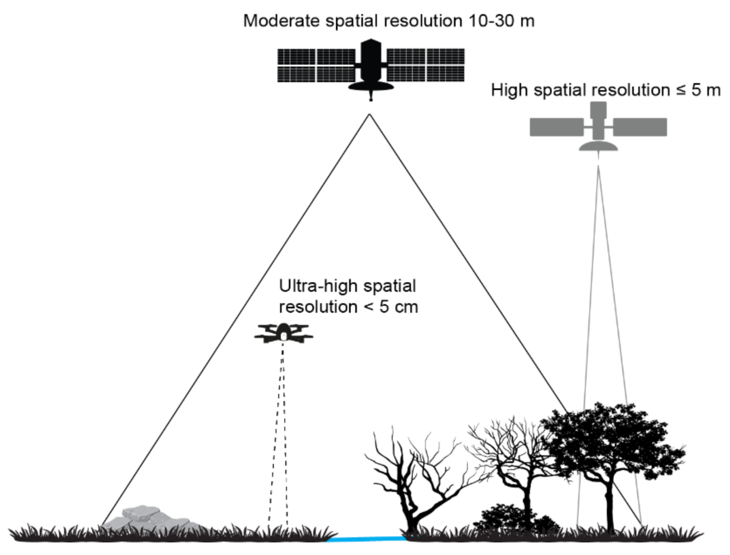
• planning for an appropriate GSD (e.g., 1–3 cm is generally sufficient for most fine scale applications),
• understanding the relationship between focal length, sensor size and flight altitude on the expected GSD,
• understanding the importance of photograph quality and target type on the outcome of the SfM workflow (e.g., the white water rapids at Corredeira do Suplício cannot be reconstructed),
• utilizing a flight planning application and flight controller software to ensure proper front and side overlap between photographs
• understanding the impact of file type and compression of the photographs on the SfM products

Across the various commercial and open source software available for the SfM processing, a plethora of studies (e.g., [108,109,110,111,112,113,114,115]) have compared the impact of software choice, software settings, photograph pre-processing, etc., for both above and below water applications. The SfM products and datasets derived from them may become the only digital reference data to sites that are permanently modified, in this case, the rheophile habitats that no longer exist after inundation (Figure 14c and Figure 15).

Data visualization is a strength of remotely sensed data and the derived analytical products. Publicly accessible repositories and tools such as Google Earth Timelapse and Google Earth VR provide access to archives of satellite imagery for qualitative assessment and visualization without the need for storage or local analytical capabilities. In this study, both platforms highlight the intensive land cover change around the HPPS reservoir (Figure 16), and in the case of the VR visualization, the high resolution satellite imagery also illustrates the remnants of flooded forest and permanently modified tributary creeks. The point cloud generated from the SfM can be readily adapted for a more interactive user experience (e.g., Figure 17). While conventional online hosting allows the user to manipulate the model change view angle, zoom level or perspective through a basic interactive experience, the use of VR enhances the interactivity and sense of presence. While modern consumer grade systems are broadly accessible and relatively low cost, there are however, more cost-efficient alternatives such as Google Cardboard compatible viewers which incorporate most smartphones to project the data. For remote or difficult to access locations, examination of field sites under restrictions as faced by the global pandemic, or examination of digitally preserved sites that no longer exist, VR has increased value. VR not only increases the understanding of place, but can also help develop fieldwork observational techniques, while developing data interpretation skills of increasing importance in the future [116]. Virtual reality allows users to interact with the models and not only gain a more real sense of the study site, but also raise broader interest in the project [117].

5. Conclusions

The licensing process in Brazil requires an environmental impact study (EIA) [118]. However, environmental impact studies are generally not standardized and none of the studies carried out on the dams of the Teles Pires assessed the structural complexity of the river substrate and the potential loss of micro-habitats. We advocate that standardized freshwater habitat classifications generated from remotely sensed data should be included in every hydroelectric EIA. The studies should not rely on pre-existing classifications which are too coarse and often inaccurate in quantifying the aquatic-terrestrial boundaries and precise land covers in the planned lentic zones [5,16]. Frequent revisit period, high spatial resolution satellite imagery provides a better choice of data from which to derive landscape classifications for use in dam construction planning and EIAs.

While the negative effects of the ongoing expansion of hydroelectric dams in Brazil and elsewhere in the Amazon on migratory fishes has been well documented, dams have other equally devastating effects on biodiversity such as the loss of specialized habitat for rheophile species, or those restricted to the unique conditions of the small creek tributaries. Their contributions to long-term GHG emissions have also become increasingly popular areas of study for installations around the world. Multi-scale remote sensing from satellite imagery to UAS platforms can provide data products to facilitate long-term monitoring and assessment of hydropower dams and their impacts on the regional landscape, as well as unique micro-habitats important for many species.

References

1. Rose, R.A.; Byler, D.; Eastman, J.R.; Fleishman, E.; Geller, G.; Goetz, S.; Guild, L.; Hamilton, H.; Hansen, M.; Headley, R.; et al. Ten ways remote sensing can contribute to conservation. Conserv. Biol. 2015, 29, 350–359. [Google Scholar] [CrossRef] [PubMed] [Green Version]
2. Arvor, D.; Dubreuil, V.; Simoes, M.; Begue, A. Mapping and spatial analysis of the soybean agricultural frontier in Mato Grosso, Brazil, using remote sensing data. Geojournal 2013, 78, 833–850. [Google Scholar] [CrossRef] [Green Version]
3. Sano, E.E.; Rodrigues, A.A.; Martins, E.S.; Bettiol, G.M.; Bustamante, M.M.C.; Bezerra, A.S.; Couto, A.F., Jr.; Vasconcelos, V.; Schuler, J.; Bolfe, E.L. Cerrado ecoregions: A spatial framework to assess and prioritize Brazilian savanna environmental diversity for conservation. J. Environ. Manag. 2019, 232, 818–828. [Google Scholar] [CrossRef] [PubMed]
4. Diniz, C.G.; Souza, A.A.d.A.; Santos, D.C.; Dias, M.C.; Luz, N.C.d.; Moraes, D.R.V.d.; Maia, J.S.A.; Gomes, A.R.; Narvaes, I.d.S.; Valeriano, D.M.; et al. DETER-B: The New Amazon Near Real-Time Deforestation Detection System. IEEE J. Sel. Top. Appl. Earth Obs. Remote Sens. 2015, 8, 3619–3628. [Google Scholar] [CrossRef]
5. Kalacska, M.; Arroyo-Mora, J.P.; Lucanus, O.; Sousa, L.; Pereira, T.; Vieira, T. Deciphering the many maps of the Xingu River Basin—An assessment of land cover classifications at multiple scales. Proc. Acad. Natl. Sci. Phila. 2020, 166, 1–55. [Google Scholar] [CrossRef]
6. Bourgoin, C.; Blanc, L.; Bailly, J.S.; Cornu, G.; Berenguer, E.; Oszwald, J.; Tritsch, I.; Laurent, F.; Hasan, A.F.; Sist, P.; et al. The Potential of Multisource Remote Sensing for Mapping the Biomass of a Degraded Amazonian Forest. Forests 2018, 9, 303. [Google Scholar] [CrossRef] [Green Version]
7. Bruno, D.E.; Ruban, D.A.; Tiess, G.; Pirrone, N.; Perrotta, P.; Mikhailenko, A.V.; Ermolaev, V.A.; Yashalova, N.N. Artisanal and small-scale gold mining, meandering tropical rivers, and geological heritage: Evidence from Brazil and Indonesia. Sci. Total Environ. 2020, 715, 136907. [Google Scholar] [CrossRef]
8. Silva Rotta, L.H.; Alcântara, E.; Park, E.; Negri, R.G.; Lin, Y.N.; Bernardo, N.; Mendes, T.S.G.; Souza Filho, C.R. The 2019 Brumadinho tailings dam collapse: Possible cause and impacts of the worst human and environmental disaster in Brazil. Int. J. Appl. Earth Obs. Geoinf. 2020, 90, 102119. [Google Scholar] [CrossRef]
9. Rudorff, N.; Rudorff, C.M.; Kampel, M.; Ortiz, G. Remote sensing monitoring of the impact of a major mining wastewater disaster on the turbidity of the Doce River plume off the eastern Brazilian coast. ISPRS J. Photogramm. Remote Sens. 2018, 145, 349–361. [Google Scholar] [CrossRef]
10. Chen, G.; Powers, R.P.; de Carvalho, L.M.T.; Mora, B. Spatiotemporal patterns of tropical deforestation and forest degradation in response to the operation of the Tucuruí hydroelectric dam in the Amazon basin. Appl. Geogr. 2015, 63, 1–8. [Google Scholar] [CrossRef]
11. Condé, R.; Martinez, J.-M.; Pessotto, M.; Villar, R.; Cochonneau, G.; Henry, R.; Lopes, W.; Nogueira, M. Indirect Assessment of Sedimentation in Hydropower Dams Using MODIS Remote Sensing Images. Remote Sens. 2019, 11, 314. [Google Scholar] [CrossRef] [Green Version]
12. Skole, D.; Tucker, C. Tropical deforestation and habitat fragmentation in the Amazon: Satellite data from 1978 to 1988. Science 1993, 260, 1905–1910. [Google Scholar] [CrossRef] [PubMed] [Green Version]
13. Silva, S.S.D.; Oliveira, I.; Morello, T.F.; Anderson, L.O.; Karlokoski, A.; Brando, P.M.; Melo, A.W.F.; Costa, J.G.D.; Souza, F.S.C.; Silva, I.S.D.; et al. Burning in southwestern Brazilian Amazonia, 2016–2019. J. Environ. Manag. 2021, 286, 112189. [Google Scholar] [CrossRef]
14. Escobar, H. Brazil’s Deforestation Is Exploding—And 2020 Will Be Worse. Available online: https://www.sciencemag.org/news/2019/11/brazil-s-deforestation-exploding-and-2020-will-be-worse (accessed on 23 January 2021).
15. Escobar, H. Deforestation in the Amazon is shooting up, but Brazil’s president calls the data ‘a lie’. Available online: https://www.sciencemag.org/news/2019/07/deforestation-amazon-shooting-brazil-s-president-calls-data-lie (accessed on 23 January 2021).
16. Kalacska, M.; Lucanus, O.; Sousa, L.; Arroyo-Mora, J.P. High-Resolution Surface Water Classifications of the Xingu River, Brazil, Pre and Post Operationalization of the Belo Monte Hydropower Complex. Data 2020, 5, 75. [Google Scholar] [CrossRef]
17. Asner, G.P. Cloud cover in Landsat observations of the Brazilian Amazon. Int. J. Remote Sens. 2001, 22, 3855–3862. [Google Scholar] [CrossRef]
18. Adriano, B.; Xia, J.; Baier, G.; Yokoya, N.; Koshimura, S. Multi-Source Data Fusion Based on Ensemble Learning for Rapid Building Damage Mapping during the 2018 Sulawesi Earthquake and Tsunami in Palu, Indonesia. Remote Sens. 2019, 11, 886. [Google Scholar] [CrossRef] [Green Version]
19. Niroumand-Jadidi, M.; Bovolo, F.; Bruzzone, L.; Gege, P. Physics-based Bathymetry and Water Quality Retrieval Using PlanetScope Imagery: Impacts of 2020 COVID-19 Lockdown and 2019 Extreme Flood in the Venice Lagoon. Remote Sens. 2020, 12, 2381. [Google Scholar] [CrossRef]
20. Cheng, Y.; Vrieling, A.; Fava, F.; Meroni, M.; Marshall, M.; Gachoki, S. Phenology of short vegetation cycles in a Kenyan rangeland from PlanetScope and Sentinel-2. Remote Sens. Environ. 2020, 248, 112004. [Google Scholar] [CrossRef]
21. Crutsinger, G.; Short, J.; Sollendberger, R. The future of UAVs in ecology: An insider perspective from the Silicon Valley drone industry. J. Unmanned Veh. Syst. 2016, 4, 161–168. [Google Scholar] [CrossRef] [Green Version]
22. Ridge, J.T.; Johnston, D.W. Unoccupied Aircraft Systems (UAS) for Marine Ecosystem Restoration. Front. Mar. Sci. 2020, 7, 438. [Google Scholar] [CrossRef]
23. Arroyo-Mora, J.P.; Kalacska, M.; Løke, T.; Schläpfer, D.; Coops, N.C.; Lucanus, O.; Leblanc, G. Assessing the impact of illumination on UAV pushbroom hyperspectral imagery collected under various cloud cover conditions. Remote Sens. Environ. 2021, 258, 112396. [Google Scholar] [CrossRef]
24. Kalacska, M.; Lucanus, O.; Arroyo-Mora, J.P.; Laliberté, É.; Elmer, K.; Leblanc, G.; Groves, A. Accuracy of 3D Landscape Reconstruction without Ground Control Points Using Different UAS Platforms. Drones 2020, 4, 13. [Google Scholar] [CrossRef] [Green Version]
25. Fonstad, M.A.; Dietrich, J.T.; Courville, B.C.; Jensen, J.L.; Carbonneau, P.E. Topographic structure from motion: A new development in photogrammetric measurement. Earth Surf. Process. Landf. 2013, 38, 421–430. [Google Scholar] [CrossRef] [Green Version]
26. Micheletti, N.; Chandler, J.H.; Lane, S.N. Investigating the geomorphological potential of freely available and accessible structure-from-motion photogrammetry using a smartphone. Earth Surf. Process. Landf. 2015, 40, 473–486. [Google Scholar] [CrossRef] [Green Version]
27. Carrivick, J.; Smith, M. Fluvial and aquatic applications of Structure from Motion photogrammetry and unmanned aerial vehicle/drone technology. WIREs Water 2018, 6, e1328. [Google Scholar] [CrossRef] [Green Version]
28. Shintani, C.; Fonstad, M.A. Comparing remote-sensing techniques collecting bathymetric data from a gravel-bed river. Int. J. Remote Sens. 2017, 38, 2883–2902. [Google Scholar] [CrossRef]
29. Kalacska, M.; Lucanus, O.; Sousa, L.; Vieira, T.; Arroyo-Mora, J.P. Freshwater Fish Habitat Complexity Mapping Using Above and Underwater Structure-From-Motion Photogrammetry. Remote Sens. 2018, 10, 1912. [Google Scholar] [CrossRef] [Green Version]
30. Zarfl, C.; Lumsdon, A.E.; Berlekamp, J.; Tydecks, L.; Tockner, K. A global boom in hydropower dam construction. Aquat. Sci. 2015, 77, 161–170. [Google Scholar] [CrossRef]
31. Winemiller, K.O.; McIntyre, P.B.; Castello, L.; Fluet-Chouinard, E.; Giarrizzo, T.; Nam, S.; Baird, I.G.; Darwall, W.; Lujan, N.K.; Harrison, I.; et al. Balancing hydropower and biodiversity in the Amazon, Congo, and Mekong. Science 2016, 351, 128–129. [Google Scholar] [CrossRef] [Green Version]
32. Couto, T.B.A.; Olden, J.D. Global proliferation of small hydropower plants—Science and policy. Front. Ecol. Environ. 2018, 16, 91–100. [Google Scholar] [CrossRef]
33. Lin, Z.; Qi, J. A New Remote Sensing Approach to Enrich Hydropower Dams’ Information and Assess Their Impact Distances: A Case Study in the Mekong River Basin. Remote Sens. 2019, 11, 3016. [Google Scholar] [CrossRef] [Green Version]
34. Couto, T.B.A.; Messager, M.L.; Olden, J.D. Safeguarding migratory fish via strategic planning of future small hydropower in Brazil. Nat. Sustain. 2021, 4, 409–416. [Google Scholar] [CrossRef]
35. Latrubesse, E.M.; Arima, E.Y.; Dunne, T.; Park, E.; Baker, V.R.; d’Horta, F.M.; Wight, C.; Wittmann, F.; Zuanon, J.; Baker, P.A.; et al. Damming the rivers of the Amazon basin. Nature 2017, 546, 363–369. [Google Scholar] [CrossRef] [PubMed]
36. Timpe, K.; Kaplan, D. The changing hydrology of a dammed Amazon. Sci. Adv. 2017, 3. [Google Scholar] [CrossRef] [PubMed] [Green Version]
37. Agostinho, A.A.; Pelicice, F.M.; Gomes, L.C. Dams and the fish fauna of the Neotropical region: Impacts and management related to diversity and fisheries. Braz. J. Biol. 2008, 68, 1119–1132. [Google Scholar] [CrossRef] [Green Version]
38. Cella-Ribeiro, A.; Doria, C.R.D.; Dutka-Gianelli, J.; Alves, H.; Torrente-Vilara, G. Temporal fish community responses to two cascade run-of-river dams in the Madeira River, Amazon basin. Ecohydrology 2017, 10, e1889. [Google Scholar] [CrossRef]
39. Hickford, M.J.H.; Schiel, D.R. Population sinks resulting from degraded habitats of an obligate life-history pathway. Oecologia 2011, 166, 131–140. [Google Scholar] [CrossRef]
40. Rosa, C.; Secco, H.; Silva, L.G.; Lima, M.G.; Gordo, M.; Magnusson, W. Burying water and biodiversity through road constructions in Brazil. Aquat. Conserv. Mar. Freshw. Ecosyst. 2021. [Google Scholar] [CrossRef]
41. Roussel, J.-M.; Covain, R.; Vigouroux, R.; Allard, L.; Treguier, A.; Papa, Y.; Le Bail, P.-Y. Fish communities critically depend on forest subsidies in small neotropical streams with high biodiversity value. Biotropica 2021. [Google Scholar] [CrossRef]
42. Gunkel, G. Hydropower—A Green Energy? Tropical Reservoirs and Greenhouse Gas Emissions. CLEAN Soil Air Water 2009, 37, 726–734. [Google Scholar] [CrossRef]
43. Almeida, R.M.; Shi, Q.; Gomes-Selman, J.M.; Wu, X.; Xue, Y.; Angarita, H.; Barros, N.; Forsberg, B.R.; Garcia-Villacorta, R.; Hamilton, S.K.; et al. Reducing greenhouse gas emissions of Amazon hydropower with strategic dam planning. Nat. Commun. 2019, 10, 4281. [Google Scholar] [CrossRef] [PubMed]
44. Fricke, R.; Eschmeyer, W.N.; vander Laan, R. Eschmeyer’s Catalog of Fishes: Genera, Species, References. Available online: http://researcharchive.calacademy.org/research/ichthyology/catalog/fishcatmain.asp (accessed on 1 March 2021).
45. Jezequel, C.; Tedesco, P.A.; Darwall, W.; Dias, M.S.; Frederico, R.G.; Hidalgo, M.; Hugueny, B.; Maldonado-Ocampo, J.; Martens, K.; Ortega, H.; et al. Freshwater fish diversity hotspots for conservation priorities in the Amazon Basin. Conserv. Biol. 2020, 34, 956–965. [Google Scholar] [CrossRef] [PubMed]
46. Jezequel, C.; Tedesco, P.A.; Bigorne, R.; Maldonado-Ocampo, J.A.; Ortega, H.; Hidalgo, M.; Martens, K.; Torrente-Vilara, G.; Zuanon, J.; Acosta, A.; et al. A database of freshwater fish species of the Amazon Basin. Sci. Data 2020, 7, 1–9. [Google Scholar] [CrossRef] [Green Version]
47. Fearnside, P.M. Belo Monte: Actors and arguments in the struggle over Brazil’s most controversial Amazonian dam. Die Erde 2017, 148, 14–26. [Google Scholar] [CrossRef]
48. Fearnside, P.M. Brazil’s Belo Monte Dam: Lessons of an Amazonian resource struggle. Die Erde 2017, 2–3, 167–184. [Google Scholar] [CrossRef]
49. Fearnside, P.M. Amazon dams and waterways: Brazil’s Tapajos Basin plans. Ambio 2015, 44, 426–439. [Google Scholar] [CrossRef] [PubMed] [Green Version]
50. Arima, E.Y.; Walker, R.T.; Perz, S.; Souza, C. Explaining the fragmentation in the Brazilian Amazonian forest. J. Land Use Sci. 2016, 11, 257–277. [Google Scholar] [CrossRef]
51. Fearnside, P.M.; Graca, P. BR-319: Brazil’s Manaus-Porto Velho highway and the potential impact of linking the arc of deforestation to central Amazonia. Environ. Manag. 2006, 38, 705–716. [Google Scholar] [CrossRef]
52. Nepstad, D.; McGrath, D.; Stickler, C.; Alencar, A.; Azevedo, A.; Swette, B.; Bezerra, T.; DiGiano, M.; Shimada, J.; Seroa da Motta, R.; et al. Slowing Amazon deforestation through public policy and interventions in beef and soy supply chains. Science 2014, 344, 1118. [Google Scholar] [CrossRef]
53. Espíndola, V.C.; Spencer, M.R.S.; Rocha, L.R.; Britto, M.R. A new species of Corydoras Lacépède (Siluriformes: Callichthyidae) from the Rio Tapajós basin and its phylogenetic implications. Papéis Avulsos Zool. (São Paulo) 2014, 54, 25–32. [Google Scholar] [CrossRef] [Green Version]
54. Barthem, R.; Goulding, M. The Catfish Connection: Ecology, Migration, and Conservation of Amazon; Columbia University Press: New York, NY, USA, 1997. [Google Scholar]
55. Hrbek, T.; Meliciano, N.V.; Zuanon, J.; Farias, I.P. Remarkable Geographic Structuring of Rheophilic Fishes of the Lower Araguaia River. Front. Genet. 2018, 9, 295. [Google Scholar] [CrossRef] [Green Version]
56. Matos, L.S.; Santana, H.S.; Silva, J.O.S.; Carvalho, L.N. Perception of professional artesanal fishermen on the decline in the catch of matrinxa fish in the Teles Pires River, Tapajos Basin. In Padroes Ambientais Emergentes e Sustentabilidade dos Sistemas; Prandel, J.A., Ed.; Atena Editora: Ponta Grossa, PR, Brazil, 2020. [Google Scholar] [CrossRef]
57. Santos, J.; Correa, S.B.; Boudreau, M.R.; Carvalho, L.N. Differential ontogenetic effects of gut passage through fish on seed germination. Acta Oecol. 2020, 108, 103628. [Google Scholar] [CrossRef]
58. Planet Labs Inc. RapidEye, A.G. Satellite Imagery Product Specifications. Available online: https://www.planet.com/products/satellite-imagery/files/160625-RapidEyeImage-Product-Specifications.pdf (accessed on 23 January 2021).
59. Planet Labs Inc. Our Approach. Available online: https://www.planet.com/company/approach/ (accessed on 22 April 2021).
60. Planet Labs Inc. Planet Imagery Product Specification: PlanetScope & RapidEye. Available online: https://www.planet.com/products/satellite-imagery/files/1610.06_SpecSheet_Combined_Imagery_Product_Letter_ENGv1.pdf (accessed on 23 January 2021).
61. Chen, G.; Weng, Q.H.; Hay, G.J.; He, Y.N. Geographic object-based image analysis (GEOBIA): Emerging trends and future opportunities. GISci. Remote Sens. 2018, 55, 159–182. [Google Scholar] [CrossRef]
62. Johnson, B.A.; Ma, L. Image Segmentation and Object-Based Image Analysis for Environmental Monitoring: Recent Areas of Interest, Researchers’ Views on the Future Priorities. Remote Sens. 2020, 12, 1772. [Google Scholar] [CrossRef]
63. Johansen, K.; Sallam, N.; Robson, A.; Samson, P.; Chandler, K.; Derby, L.; Eaton, A.; Jennings, J. Using GeoEye-1 Imagery for Multi-Temporal Object-Based Detection of Canegrub Damage in Sugarcane Fields in Queensland, Australia. GISci. Remote Sens. 2018, 55, 285–305. [Google Scholar] [CrossRef]
64. Demarchi, L.; van de Bund, W.; Pistocchi, A. Object-Based Ensemble Learning for Pan-European Riverscape Units Mapping Based on Copernicus VHR and EU-DEM Data Fusion. Remote Sens. 2020, 12, 1222. [Google Scholar] [CrossRef] [Green Version]
65. Pix4D. Initial Processing -> Calibration. Available online: https://support.pix4d.com/hc/en-us/articles/205327965-Menu-Process-Processing-Options-1-Initial-Processing-Calibration (accessed on 22 April 2021).
66. Strecha, C.; Bronstein, A.; Bronstein, M.M.; Fua, P. LDAHash: Improved Matching with Smaller Descriptors. IEEE Trans. Pattern Anal. Mach. Intell. 2012, 34, 66–78. [Google Scholar] [CrossRef] [PubMed] [Green Version]
67. Strecha, C.; Kung, O.; Fua, P. Automatic mapping from ultra-light UAV imagery. In Proceedings of the 2012 European Calibration and Orientation Workshop, Barcelona, Spain, 8–10 February 2012; pp. 1–4. [Google Scholar]
68. Strecha, C.; von Hansen, W.; Van Gool, L.; Fua, P.; Thoennessen, U. On Benchmarking camera calibration and multi-view stereo for high resolution imagery. In Proceedings of the IEEE Conference on Computer Vision and Pattern Recognition, Anchorage, AK, USA, 23–28 June 2008. [Google Scholar]
69. Shumway, C.A.; Hofmann, H.A.; Dobberfuhl, A.P. Quantifying habitat complexity in aquatic ecosystems. Freshw. Biol. 2007, 52, 1065–1076. [Google Scholar] [CrossRef]
70. St. Pierre, J.I.; Kovalenko, K.E. Effect of habitat complexity attributes on species richness. Ecosphere 2014, 5, art22. [Google Scholar] [CrossRef]
71. McCormick, M.I. Comparison of field methods for measuring surface topography and their associations with a tropical reef fish assemblage. Mar. Ecol. Prog. Ser. 1994, 112, 87–96. [Google Scholar] [CrossRef]
72. Walbridge, S.; Slocum, N.; Pobuda, M.; Wright, D.M. Unified Geomorphological Analysis Workflows with Benthic Terrain Modeler. Geosciences 2018, 8, 94. [Google Scholar] [CrossRef] [Green Version]
73. Sappington, J.; Longshore, K.; Thompson, D. Quantifying Landscape Ruggedness for Animal Habitat Analysis: A Case Study Using Bighorn Sheep in the Mojave Desert. J. Wildl. Manag. 2007, 71, 1419–1426. [Google Scholar] [CrossRef]
74. Backes, A.R.; Eler, D.M.; Minghim, R.; Bruno, O.M. Characterizing 3D shapes using fractal dimension. In Progress in Pattern Recognition, Image Analysis, Computer Vision, and Applications SE-7; Bloch, I., Cesar, R., Jr., Eds.; Springer: Heidelberg, Germany, 2012; pp. 14–21. [Google Scholar]
75. Reichert, J.; Backes, A.R.; Schubert, P.; Wilke, T.; Mahon, A. The power of 3D fractal dimensions for comparative shape and structural complexity analyses of irregularly shaped organisms. Methods Ecol. Evol. 2017, 8, 1650–1658. [Google Scholar] [CrossRef]
76. Simard, M.; Pinto, N.; Fisher, J.B.; Baccini, A. Mapping forest canopy height globally with spaceborne lidar. J. Geophys. Res. 2011, 116. [Google Scholar] [CrossRef] [Green Version]
77. Spawn, S.A.; Sullivan, C.C.; Lark, T.J.; Gibbs, H.K. Harmonized global maps of above and belowground biomass carbon density in the year 2010. Sci. Data 2020, 7, 112. [Google Scholar] [CrossRef]
78. Spawn, S.A.; Gibbs, H.K. Global Aboveground and Belowground Biomass Carbon Density Maps for the Year 2010; ORNL DAAC: Oak Ridge, TN, USA, 2020.
79. Lorente, A.; Borsdorff, T.; Butz, A.; Hasekamp, O.; aan de Brugh, J.; Schneider, A.; Wu, L.H.; Hase, F.; Kivi, R.; Wunch, D.; et al. Methane retrieved from TROPOMI: Improvement of the data product and validation of the first 2 years of measurements. Atmos. Meas. Tech. 2021, 14, 665–684. [Google Scholar] [CrossRef]
80. Hasekamp, O.; Lorente, A.; Hu, H.; Butz, A.; aan de Brugh, J.; Landgraf, J. Algorithm Theoretical Baseline Document for Sentinel-5 Precursor Methane Retrieval. Available online: http://www.tropomi.eu/sites/default/files/files/publicSentinel-5P-TROPOMI-ATBD-Methane-retrieval.pdf (accessed on 22 April 2021).
81. Buchwitz, M.; Schneising, O.; Reuter, M.; Heymann, J.; Krautwurst, S.; Bovensmann, H.; Burrows, J.P.; Boesch, H.; Parker, R.J.; Somkuti, P.; et al. Satellite-derived methane hotspot emission estimates using a fast data-driven method. Atmos. Chem. Phys. 2017, 17, 5751–5774. [Google Scholar] [CrossRef] [Green Version]
82. Muñoz Sabater, J. ERA5-Land Monthly Averaged Data from 1981 to Present. Copernicus Climate Change Service (C3S) Climate Data Store (CDS). Available online: https://doi.org/10.24381/cds.68d2bb30 (accessed on 16 May 2021).
83. Liberatore, M.J.; Wagner, W.P. Virtual, mixed, and augmented reality: A systematic review for immersive systems research. Virtual Real. 2021. [Google Scholar] [CrossRef]
84. Yeung, A.W.K.; Tosevska, A.; Klager, E.; Eibensteiner, F.; Laxar, D.; Stoyanov, J.; Glisic, M.; Zeiner, S.; Kulnik, S.T.; Crutzen, R.; et al. Virtual and Augmented Reality Applications in Medicine: Analysis of the Scientific Literature. J. Med. Internet Res. 2021, 23, e25499. [Google Scholar] [CrossRef] [PubMed]
85. Leigh, C.; Heron, G.; Wilson, E.; Gregory, T.; Clifford, S.; Holloway, J.; McBain, M.; Gonzalez, F.; McGree, J.; Brown, R.; et al. Using virtual reality and thermal imagery to improve statistical modelling of vulnerable and protected species. PLoS ONE 2019, 14, e0217809. [Google Scholar] [CrossRef] [PubMed] [Green Version]
86. Billen, M.I.; Kreylos, O.; Hamann, B.; Jadamec, M.A.; Kellogg, L.H.; Staadt, O.; Sumner, D.Y. A geoscience perspective on immersive 3D gridded data visualization. Comput. Geosci. 2008, 34, 1056–1072. [Google Scholar] [CrossRef] [Green Version]
87. Sinop Energia. Sinop HPP. Available online: https://www.sinopenergia.com.br/ (accessed on 22 April 2021).
88. Kalacska, M.; Lucanus, O.; Sousa, L.; Arroyo-Mora, J.P. A New Multi-Temporal Forest Cover Classification for the Xingu River Basin, Brazil. Data 2019, 4, 114. [Google Scholar] [CrossRef] [Green Version]
89. Athayde, S.; Mathews, M.; Bohlman, S.; Brasil, W.; Doria, C.R.C.; Dutka-Gianelli, J.; Fearnside, P.M.; Loiselle, B.; Marques, E.E.; Melis, T.S.; et al. Mapping research on hydropower and sustainability in the Brazilian Amazon: Advances, gaps in knowledge and future directions. Curr. Opin. Environ. Sustain. 2019, 37, 50–69. [Google Scholar] [CrossRef]
90. Deemer, B.R.; Harrison, J.A.; Li, S.; Beaulieu, J.J.; DelSontro, T.; Barros, N.; Bezerra-Neto, J.F.; Powers, S.M.; Dos Santos, M.A.; Vonk, J.A. Greenhouse Gas Emissions from Reservoir Water Surfaces: A New Global Synthesis. Bioscience 2016, 66, 949–964. [Google Scholar] [CrossRef] [PubMed]
91. Kemenes, A.; Forsberg, B.R.; Melack, J.M. CO2 emissions from a tropical hydroelectric reservoir (Balbina, Brazil). J. Geophys. Res. 2011, 116. [Google Scholar] [CrossRef] [Green Version]
92. Demarty, M.; Bastien, J. GHG emissions from hydroelectric reservoirs in tropical and equatorial regions: Review of 20 years of CH4 emission measurements. Energy Policy 2011, 39, 4197–4206. [Google Scholar] [CrossRef]
93. Potter, C.; Brooks-Genovese, V.; Klooster, S.; Torregrosa, A. Biomass burning emissions of reactive gases estimated from satellitedata analysis and ecosystem modeling for the Brazilian Amazon region. J. Geophys. Res. 2002, 107, 8056. [Google Scholar] [CrossRef] [Green Version]
94. de Araújo, K.R.; Sawakuchi, H.O.; Bertassoli Jr, D.J.; Sawakuchi, A.O.; da Silva, K.D.; Vieira, T.B.; Ward, N.D.; Pereira, T.S. Carbon dioxide (CO2) concentrations and emission in the newly constructed Belo Monte hydropower complex in the Xingu River, Amazonia. Biogeosciences 2019, 16, 3527–3542. [Google Scholar] [CrossRef] [Green Version]
95. de Faria, F.A.M.; Jaramillo, P.; Sawakuchi, H.O.; Richey, J.E.; Barros, N. Estimating greenhouse gas emissions from future Amazonian hydroelectric reservoirs. Environ. Res. Lett. 2015, 10, 124019. [Google Scholar] [CrossRef] [Green Version]
96. Swanson, A.C.; Bohlman, S. Cumulative Impacts of Land Cover Change and Dams on the Land–Water Interface of the Tocantins River. Front. Environ. Sci. 2021, 9, 120. [Google Scholar] [CrossRef]
97. Cabeceira, F. Relações Entre Estrutura do Habitat, Composição Taxonômica e Trófica de Peixes em Riachos da Bacia do rio Teles Pires, Amazônia. Meridional. Thesis, Universidade Federal de Mato Grosso, Cuiabá, Brazil, 2014. [Google Scholar]
98. Wertheimer, R.H.; Evans, A.F. Downstream passage of steelhead kelts through hydroelectric dams on the Lower Snake and Columbia Rivers. Trans. Am. Fish. Soc. 2005, 134, 853–865. [Google Scholar] [CrossRef]
99. Ohara, W.M.; Lima, F.C.T.; Salvador, G.N.; Andrade, M.C. Peixes do rio Teles Pires: Diversidade e Guia de Identificação; Gráfica e Editora Amazonas: Goiânia, Brazil, 2017; p. 408. [Google Scholar]
100. Ram, H.Y.M.; Sehgal, A.; ZSI. Podostemaceae—An Evolutionary Enigma; Zoological Survey India: Calcutta, India, 2007; pp. 37–66. [Google Scholar]
101. Cunliffe, A.M.; Brazier, R.E.; Anderson, K. Ultra-fine grain landscape-scale quantification of dryland vegetation structure with drone-acquired structure-from-motion photogrammetry. Remote Sens. Environ. 2016, 183, 129–143. [Google Scholar] [CrossRef] [Green Version]
102. Chirayath, V.; Instrella, R. Fluid lensing and machine learning for centimeter-resolution airborne assessment of coral reefs in American Samoa. Remote Sens. Environ. 2019, 235. [Google Scholar] [CrossRef]
103. Fraser, B.T.; Congalton, R.G. Issues in Unmanned Aerial Systems (UAS) data collection of complex forest environments. Remote Sens. 2018, 10, 908. [Google Scholar] [CrossRef] [Green Version]
104. Joyce, K.E.; Duce, S.; Leahy, S.M.; Leon, J.; Maier, S.W. Principles and practice of acquiring drone-based image data in marine environments. Mar. Freshw. Res. 2019, 70, 952–963. [Google Scholar] [CrossRef]
105. Resop, J.P.; Lehmann, L.; Hession, W.C. Drone laser scanning for modeling riverscape topography and vegetation: Comparison with traditional aerial LiDAR. Drones 2019, 3, 35. [Google Scholar] [CrossRef] [Green Version]
106. Ventura, D.; Dubois, S.F.; Bonifazi, A.; Lasinio, G.J.; Seminara, M.; Gravina, M.F.; Ardizzone, G. Integration of close-range underwater photogrammetry with inspection and mesh processing software: A novel approach for quantifying ecological dynamics of temperate biogenic reefs. Remote Sens. Ecol. Conserv. 2021. [Google Scholar] [CrossRef]
107. Woodget, A.S.; Austrums, R.; Maddock, I.P.; Habit, E. Drones and digital photogrammetry: From classifications to continuums for monitoring river habitat and hydromorphology. Wiley Interdiscip. Rev. Water 2017, 4. [Google Scholar] [CrossRef] [Green Version]
108. Bianco, S.; Ciocca, G.; Marelli, D. Evaluating the performance of Structure from Motion pipelines. J. Imaging 2018, 4, 98. [Google Scholar] [CrossRef] [Green Version]
109. Dering, G.M.; Micklethwaite, S.; Thiele, S.T.; Vollgger, S.A.; Cruden, A.R. Review of drones, photogrammetry and emerging sensor technology for the study of dykes: Best practises and future potential. J. Volcanol. Geotherm. Res. 2019, 373, 148–166. [Google Scholar] [CrossRef]
110. Gomez-Gutierrez, A.; de Sanjose-Blasco, J.J.; Lozano-Parra, J.; Berenguer-Sempere, F.; de Matias-Bejarano, J. Does HDR pre-processing improve the accuracy of 3D models obtained by means of two conventional SfM-MVS software packages? The case of the Corral del Veleta rock glacier. Remote Sens. 2015, 7, 10269–10294. [Google Scholar] [CrossRef] [Green Version]
111. Mikita, T.; Balkova, M.; Bajer, A.; Cibulka, M.; Patocka, Z. Comparison of different remote sensing methods for 3D modeling of small rock outcrops. Sensors 2020, 20, 1663. [Google Scholar] [CrossRef] [PubMed] [Green Version]
112. Mousavi, V.; Khosravi, M.; Ahmadi, M.; Noori, N.; Naveh, A.H.; Varshosaz, M. The performance evaluation of multi-image 3D reconstruction software with different sensors. In International Conference on Sensors & Models in Remote Sensing & Photogrammetry; Arefi, H., Motagh, M., Eds.; EBSCO Industries, Inc.: East Birmingham, AL, USA, 2015; Volume 41, pp. 515–519. [Google Scholar]
113. Niederheiser, R.; Mokros, M.; Lange, J.; Petschko, H.; Prasicek, G.; Elberink, S.O. Deriving 3D point clouds from terrestrial photographs comparison of different sensors and software. In XXIII ISPRS Congress; Commission, V., Halounova, L., Safar, V., Remondino, F., Hodac, J., Pavelka, K., Shortis, M., Rinaudo, F., Scaioni, M., Boehm, J., et al., Eds.; 2016; Volume 41, pp. 685–692. Available online: https://www.researchgate.net/profile/Martin-Mokros/publication/307530339_DERIVING_3D_POINT_CLOUDS_FROM_TERRESTRIAL_PHOTOGRAPHS_-_COMPARISON_OF_DIFFERENT_SENSORS_AND_SOFTWARE/links/57c95a1308aedb6d6d978bab/DERIVING-3D-POINT-CLOUDS-FROM-TERRESTRIAL-PHOTOGRAPHS-COMPARISON-OF-DIFFERENT-SENSORS-AND-SOFTWARE.pdf (accessed on 16 May 2021).
114. Schoning, J.; Heidemann, G. Evaluation of multi-view 3D reconstruction software. In Computer Analysis of Images and Patterns, Caip 2015, Pt II; Azzopardi, G., Petkov, N., Eds.; Springer: New York, NY, USA, 2015; Volume 9257, pp. 450–461. [Google Scholar]
115. Vlachos, M.; Berger, L.; Mathelier, R.; Agrafiotis, P.; Skarlatos, D. Software comparison for underwater archaeological photogrammetric applications. In 27th CIPA International Symposium: Documenting the Past for a Better Future; Gonzalez Aguilera, D., Remondino, F., Toschi, I., Rodriguez Gonzalvez, P., Stathopoulou, E., Eds.; Cyprus University of Technology: Limassol, Cyprus, 2019; Volume 42-2, pp. 1195–1201. [Google Scholar]
116. Bos, D.; Miller, S.; Bull, E. Using virtual reality (VR) for teaching and learning in geography: Fieldwork, analytical skills, and employability. J. Geogr. High. Educ. 2021, 10, 1–10. [Google Scholar] [CrossRef]
117. Kalacska, M.; Arroyo-Mora, J.P.; Lucanus, O. Comparing UAS LiDAR and Structure-from-Motion Photogrammetry for peatland mapping and virtual reality (VR) visualization. Drones 2021, 5, 36. [Google Scholar] [CrossRef]
118. Fearnside, P.M. Brazil’s Sao Luiz do Tapajos Dam: The Art of Cosmetic Environmental Impact Assessments. Water Altern. Interdiscip. J. Water Politics Dev. 2015, 8, 373–396. [Google Scholar]
Figure 1. Illustration of the different levels of spatial detail that can be resolved by satellite and UAS platforms. The moderate resolution systems include common satellite-based sensors such as the CBERS (China–Brazil Earth Resources Satellite), Landsat and Sentinel-2 group of systems. The high spatial resolution systems include common satellite-based sensors such as RapidEye, Worldview and Planet Dove constellations and systems. The UAS represented refers to low-altitude systems (<100 m AGL).
Earth 02 00018 g001
Figure 2. Sector of the Teles Pires river (Mato Grosso, Brazil) impacted by the HPPS reservoir. The river’s course is shown in blue prior to the construction of the dam. The red dot indicates the location of the UAS study areas: (A) Corredeira do Suplício, photograph facing South and (B) Ilha do Lair, photograph facing North.
Earth 02 00018 g002
Figure 3. Photographs of one of the small creek tributaries prior to inundation from the HPPS reservoir. (A) unmodified creek on the eastern side of the Teles Pires river; (B) photograph taken a few hours after (A) at the same location illustrating sedimentation due to construction upstream; (C) Curculonichthys luteofrenatus feed on algae in the current; (D) Corydoras apiaka are restricted to sandy areas of low flow in these small creeks. Both species are endemic to the small clear water tributaries of the Teles Pires, Preto and Arinos rivers [53].
Earth 02 00018 g003
Figure 4. Underwater photographs of rheophile fishes endemic to the middle Teles Pires which were found at the UAS study sites prior to inundation: Leporinus vanzoi (A), Bryconexodon trombetasi (B), Pseudancistrus kayabi (C) and Teleocichla sp. (D).
Earth 02 00018 g004
Figure 5. Flowchart summarizing the datasets and analyses used in the study. The section numbers are provided as reference for each input dataset, process and result.
Earth 02 00018 g005
Figure 6. Satellite image mosaics from 2014 (RapidEye constellation) and 2020 (PlanetScope constellation) before and after the operationalization of HPPS. Both sets of images are shown as false color composites (Near infrared/Red/Green) to differentiate the river more clearly from the landscape and minimize the impact of the smoke from fires in the south-east sector of the 2014 imagery. Both mosaics represent low water conditions in July.
Earth 02 00018 g006
Figure 7. Examples of classes selected for the land cover classification. The left panel of each pair (with the red dots) illustrates the land cover through a 33 × 33 pixel window (~1 ha) from a Dove PS image (3 m pixel size). The right panels (with the blue dots) illustrate a subset of the corresponding land cover as seen from a UAS photograph (not to scale).
Earth 02 00018 g007
Figure 8. Illustration of the SfM-MVS workflow carried out in Pix4D Mapper. The inputs to the workflow (red) were the UAS photographs. The products of interest for this study (blue) were the dense point cloud, DSM and orthomosaic.
Earth 02 00018 g008
Figure 9. Minimum extent of the HPPS lentic zone during the low water (yellow) season and land cover classes within the flooded area as determined from the 2014 RapidEye image classification. Both are shown overlain on the 2014 satellite image mosaic.
Earth 02 00018 g009
Figure 10. Estimate of forest canopy height (circa 2005) from GLAS spaceborne LiDAR [76] within the lentic zone of the HPPS during high water season. The Teles Pires river pre-inundation is shown overlain.
Earth 02 00018 g010
Figure 11. Estimated aboveground biomass C (circa 2010) [77,78] pre-inundation for the lentic zone of the HPPS during high water season. The range of biomass C for the forest class is indicated in the legend. The Teles Pires river pre-inundation is shown overlain.
Earth 02 00018 g011
Figure 12. Time sequence of satellite imagery acquired monthly over the confluence of the Rio Roquete stream and Teles Pires river from prior to inundation (December 2018) to the high-water season of February 2020. Each tile is part of the monthly minimal cloud basemap mosaics produced from the PlanetScope constellation, with the exception of three single date images denoted by *. For January 2019, a single multispectral image is shown to ensure pre-inundation conditions. The 1 February 2019 image illustrates the confluence of the rivers the day after inundation began. For December 2019, a single image was chosen because it minimized cloud cover in this small area in comparison to the global mosaic. Each tile is 57.6 km2 in area.
Earth 02 00018 g012
Figure 13. Dove PS image acquired 2 February 2021 illustrating flooding of the two UAS case study areas during high water season. The frames around the UAS photographs (also acquired in February 2021) correspond to the yellow (Ilha do Lair) and red (Corredeira do Suplício) boxes on the map. Stands of dead trees in the flooded zone can be seen from both the satellite image and in the UAS photographs.
Earth 02 00018 g013
Figure 14. (A) 5 m pixel size RapidEye imagery from July 2014 from the Corredeira do Suplício UAS study area; (B) 3 m pixel size PlanetScope imagery from September 2018 coincident with the UAS image acquisition; (C) orthomosaic the SfM-MVS workflow (2 cm pixel size) of the Corredeira do Suplício (4 September 2018). The outline of the UAS orthomosaic is shown in white in panels (A,B).
Earth 02 00018 g014
Figure 15. (A) 3D dense point cloud of the Ilha do Lair UAS case study area; (B) DSM from the subset within the red box in A. Elevation transect along the black line is also shown; (C) Vector Ruggedness calculated at a window size of 20 cm and 80 cm from the DSM. The interactive point cloud is available from: https://skfb.ly/onEEp, accessed on 29 May 2021 (VR compatible) and https://bit.ly/ilhadolair, accessed on 29 May 2021 (web based). (in Supplementary Materials).
Earth 02 00018 g015
Figure 16. (A) Screen recording illustrating the land cover change animation over the HPPS lentic zone from 1984–2020 from Google Earth Timelapse. The live link can be viewed at: https://bit.ly/3gyn5sw, accessed on 29 May 2021. (B) screen recording of the lentic zone from Google Earth VR as seen through the Oculus Quest 2.
Earth 02 00018 g016
Figure 17. Video of the Ilha do Lair dataset being viewed in VR with the Oculus Quest 2 HMD in VRifier.
Earth 02 00018 g017