Edge Computing Architecture for Optimal Settings of Inverse Time Overcurrent Relays in Mesh Microgrids

Abstract

This paper presents a novel edge-computing-based architecture for optimal inverse time overcurrent relays installed to protect mesh microgrids (MGs) with distributed generation. The procedure employs graph theory to automate the detection of network changes, fault locations, and relay pairs in an MG. In addition, an automated process obtains the initial protection settings based on the operating conditions of the MG. Furthermore, the Continuous Genetic Algorithm (CGA), Salp Swarm Algorithm (SSA), and Particle Swarm Optimization (PSO) were implemented to determine the optimal protection settings to obtain better coordination between primary and backup protection relays. These processes were implemented using PowerFactory 2024 Service Pack 5A and Python 3.13.1. The proposal was validated in 68 operating scenarios that considered the islanded and connected operation modes of the MG, charging and discharging cycles of electric vehicle stations, and the presence or absence of photovoltaic generation. The overcurrent protection relays were organized into 100 primary–backup relay pairs to ensure proper coordination and selectivity. The total miscoordination time (TMT) index was used to measure when all pairs of relays were coordinated, with a minimum time close to zero. The results of the graph theory show that all the meshes, fault locations, and relay pairs were identified in the MG. The approach successfully coordinated 100 relay pairs across 68 scenarios, demonstrating its scalability in complex real-world MGs. The automation process obtained an average TMT of 12.2%, while the optimization obtained a TMS of 91.6% with the CGA, and a TMT of 99% was obtained with the SSA and PSO, demonstrating the effectiveness of the optimization process in ensuring selectivity and appropriate fault clearing times.

1. Introduction

Microgrids (MGs) are one of the most promising technological solutions to the challenges of energy transition and decarbonization [1]. They can integrate distributed energy resources (DER), such as photovoltaic (PV), wind generation (WT), and energy storage systems (ESS), offering greater operational flexibility, environmental sustainability, and resilience under contingencies [2]. In addition, these systems can be operated while being connected to the power grid or in island mode, making them a strategic alternative to improve the reliability of residential, commercial, and industrial customers in urban and rural zones. In contexts where electricity supply is critical, the implementation of MGs facilitates more autonomous operating schemes capable of supporting priority loads and integrating energy communities based on sustainable principles.

1.1. General Problem

The integration of distributed generation (DG) and electric vehicle charging stations (EVCS) into distribution networks presents challenges in protection settings. Therefore, planning and operations must evolve to prioritize flexibility, adaptability, and advanced control systems to maintain the stability and reliability of power grids. Inverse-time overcurrent protection is widely used in these types of networks because of their simplicity and selectivity. However, these devices face difficulties with bidirectional power flow and variations in short-circuit currents. These features increase the risk of miscoordination, unnecessary tripping, and non-selective disconnections, directly affecting the service continuity and stability of the electrical system [3,4]. Consequently, critical users and sensitive infrastructure may be exposed to faults that are not immediately cleared, resulting in significant economic and security impacts.

1.2. Literature Review

The coordination of protection in an MG has been addressed using classical linear and nonlinear mathematical optimization approaches, with an emphasis on selectivity, reliability, and adaptability. Consequently, ref. [5] introduced a hybrid nonlinear mixed-integer programming (MINLP) formulation to accurately capture coupled constraints, such as coordination margins and relay setting limits, achieving high-quality solutions. However, this proposal brings significant computational costs and limited scalability as the number of relays, scenarios, and network configurations increases. In addition, graph theory is not applied to automatically identify primary–backup relay pairs and the MG topology.

In [6], the authors optimized the operating times and eliminated inconsistencies between primary–backup relay pairs. They used four variables in the problem: current setting multiplier, relay time, standard, and type of characteristic curve. This study addressed the operation of active distribution networks with DER. This involved the identification of relay pairs according to topology and fault zones and the validation of multiple scenarios through a comparative analysis with alternative algorithms. However, they excluded various tests with scenarios that consider MG operating in grid-connected and island modes, statistical robustness analysis under uncertainties, graph theory to identify fault location and primary–backup relay pairs, and a global miscoordination index to handle penalties in multiple reconfiguration scenarios.

In [7], an MG was used to coordinate dual-setting directional overcurrent relays with Mixed-Integer Nonlinear Programming (MINLP). Decisions included selecting standard inverse, very inverse, and extremely inverse curves. The study sought a coordination time interval between primary–backup relays to ensure selectivity. In the research, both grid-connected and island mode were considered. The definition of primary–backup relay was based on its directionality and connectivity. Research was limited by high computational complexity, challenges in parameter calibration, and the absence of sensitivity analysis for DER and environmental metrics. It did not use graph theory to identify primary–backup relay pairs or model network topology, lacked a formulated penalized miscoordination index, and did not include multi-scenario validation under network reconfiguration.

Another study compared metaheuristics on the IEC MG benchmark [8]. The study presented the coordination of an overcurrent relay with non-standard features, minimized the time of operation, and ensured a coordination time interval (CTI) $\ge 0.3 \mathrm{s}$ in various modes. The authors implemented a Sine Cosine Algorithm (SCA) and a modified Whale Optimization algorithm (mWOA), defined primary–backup relays by zones of the benchmark, and validated the results in DIgSILENT PowerFactory. Although this study presented new contributions, the mWOA did not always match SCA, highlighting the sensitivity of the algorithm and the need for cross-testing with statistical repeatability. Additionally, they did not integrate graph theory to identify primary–backup relay pairs, network meshes, reconfiguration, and unified multi-scenarios with penalized indices.

Another study proposed an improved walnut optimizer (IWO) with chaotic initialization and opposite mutation to avoid local optima [9]. It was validated in the IEEE 8/15/30 and New England 39-bus test system cases and compared with seven algorithms. It minimizes primary times under the CTI (0.1–0.5 s) and Time Dial Setting (TDS) and pickup setting limits. However, the study did not validate graph theory to identify primary–backup relay pairs and the topology of the network or present a validated global penalized index in multiple scenarios with network reconfigurations.

In addition, a study used the Quantum-Inspired Adaptive Walrus Optimization Algorithm (QIAWOA) to coordinate directional overcurrent relays [10]. The goal was to minimize the total operating time of all relays while ensuring proper selectivity and satisfying various constraints related to the TDS and Plug Settings (PS). The proposed method effectively manages the challenges introduced by the integration of DG and can be applied to complex, interconnected, and non-radial power networks. However, the study did not incorporate a theory graph to identify primary–backup relay pairs and network meshes. Moreover, there are no reports of optimal automation methodologies or optimization with a penalized index in scenarios involving network reconfiguration.

For photovoltaic uncertainty, ref. [11] proposed a combined characteristic curve (normally inverse, definite time, and instantaneous) for overcurrent relays to mitigate the effect of PV uncertainty on the coordination of relays. The method was evaluated in the IEEE 14-bus power system (mesh network) and the IEEE 33-node test feeder (radial network). It prioritizes curves and achieves a time reduction with selectivity. However, the study only coordinates 16 relays for the IEEE 14-bus power system as the mesh network and 32 relays for the radial network. Furthermore, the study did not present a graph theory procedure for identifying the topology, primary–backup relay pairs, and network meshes. Moreover, this study did not validate multiple scenarios with reconfiguration supported by a penalized global index.

Another study considered the effect of DER on overcurrent relays, highlighting bidirectionality, sympathetic tripping, protection blinding, loss of coordination, and transient stability [12]. It was tested on a modified IEEE 33-node test feeder, and differential, impedance-based, adaptive, and AI/signal approaches were reviewed. This provides practical guidelines for selectivity and coordination under variations in the mode and location of DER. However, this study did not contain a unified methodology or a homogeneous comparison with common metrics. In addition, the study did not provide a topological analysis of primary–backup relay pairs and mesh networks. Moreover, the study did not apply a global penalized index in multiple scenarios with reconfiguration.

In the realm of exact models, ref. [5] formulated an MILP in IEC-MG that minimizes the times to ensure selectivity and introduced the selection of IEC and IEEE curves along with TMS as a decision variable. Better coordination was observed in comparison to the use of a single standard, emphasizing that the family of curves is part of the optimum practical guidelines for selectivity and coordination under variations in the mode and location of DER. However, operational uncertainty was not modeled, and the ESS was not considered in daily operations. Furthermore, they did not employ graph theory to identify primary–backup relay pairs and mesh networks and reported a penalized index with the validation of several scenarios.

An integrated planning-protection approach was presented in [13], with two stages: first, the location/sizing of the DG/ESS (scenario programming), and then the coordination of the dual-setting overcurrent relays (DSOR) and fault current limiters (FCL) using an optimization technique, minimizing the total operation time of the dual-setting overcurrent relays while respecting the CTI and the operational limits of the DSOR and FCL. Standard deviations ≈ 1.1–1.2% and improvements in voltage deviation and losses were reported. However, they did not use graph theory to identify primary–backup relay pairs and mesh networks. The study did not explicitly incorporate a global miscoordination index with penalties that outlines multiscenario optimization with reconfiguration.

Furthermore, another study explored a decentralized adaptive scheme that estimates local Thevenin to coordinate without massive communications, mitigating blinding and sympathetic tripping in the IEEE 9-bus and 14-bus test systems (both modes) [14]. The operational resilience to topology changes and DER contributions was demonstrated. However, they did not incorporate graph theory to identify primary–backup relay pairs and mesh networks. Moreover, the study was not validated through a penalized index in multiple scenarios with reconfigurations and standardized metrics compared to other approaches.

In [15], an adaptive protection scheme based on clustering with Self-Organizing Maps (SOM) was presented, where the connected and disconnected states of the DG and EVCS were grouped according to patterns of miscoordination between relay pairs. For each cluster, the most effective scenario is selected, and the DOCR settings are transferred to the rest of the group, with sub-clustering if conflicts persist. The proposed method was validated in a modified IEEE 33-node test feeder with two EVCS and a synchronous DG, showing reductions in the average trip time and aggregate miscoordination index compared with conventional coordination, and discussing centralized (IEC-61850) or decentralized (peer-to-peer) implementations. Nevertheless, the study did not consider graph theory for identifying meshes in a network or primary–backup relay pairs. The study did not integrate optimal automation methodologies and did not articulate a multi-scenario validation with reconfiguration supported by a penalized global index. These proposals were contextualized in comprehensive reviews by refs. [3,4,16], who highlighted the need for robust and scalable methods.

Finally, a study applied graph theory to analyze failure trajectories [17], whereas Asl et al. [18] explored the counting of fundamental loops with mathematical foundations to represent complex topologies. The authors proposed a centralized protection scheme for new-energy AC microgrids, motivated by the fact that widespread renewable integration, such as photovoltaics and wind, can make the power-flow direction uncertain, undermining traditional fault-section identification. The approach relies on distributed directional protection at field terminal units and on transmitting compact logical outcomes to a central entity, rather than performing heavy computations locally. Using a graph-theoretic representation of the operating topology and a matrix-based decision process, the method determines the faulted section, including branching configurations, to accelerate fault processing and service restoration. The procedure is demonstrated on a typical microgrid configuration under both grid-connected and island modes, reporting correct identification across the illustrated fault locations. Moreover, the study was not validated through a penalized index in multiple scenarios with reconfigurations and standardized metrics compared to other approaches, and they were not fully integrated with optimization algorithms.

1.3. Literature Gap

The coordination of inverse-time overcurrent protections in mesh MGs is important to ensure the reliable and efficient operation of power grids. However, current research in this field has several limitations:

• Most studies performed optimal coordination on a limited number of relays in a mesh network without considering an automatic process to perform this task.
• In most cases, overcurrent protection coordination was evaluated for a very limited number of case studies that involved changing network scenarios.
• The literature did not show methods for identifying the network topology, fault location, and pairs of relays to coordinate. This is useful for the complete automation of protection.
• The literature shows that work has been done with offline applications and that edge computing automation and optimization processes have not been addressed.

This gap in the literature presents an opportunity to develop comprehensive methods for identifying network topologies, fault points, and relay pairs. In addition, the system can be improved by considering automation and optimization for coordinating protection systems, enabling more efficient and reliable operation. Furthermore, exploring the potential of edge computing for real-time coordination could revolutionize protection strategies in mesh networks and address the limitations of current offline applications.

1.4. Objetive and Novelty

This study introduces an edge-computing-based automation method to coordinate inverse-time overcurrent relays in meshed MGs. By integrating graph theory and optimization algorithms into an edge computing architecture, the system dynamically adjusts the relay protection settings according to the network topology, current direction, and load conditions. This improves the response to critical events and enables adaptive real-time relay coordination, particularly in MGs with DG and multiple supply paths. The proposed method employs a Continuous Genetic Algorithm (CGA), Salp Swarm Algorithm (SSA), and Particle Swarm Optimization (PSO) to minimize the global miscoordination index and achieve optimal directional overcurrent protection with minimum response times. The protection settings are updated according to changes in the load, generation, and topology, improving the resilience, operational efficiency, and selectivity.

1.5. Contributions

Table 1. Comparison of approaches and relevant findings for coordination of inverse-time overcurrent protections in mesh MGs.

Ref.	Number of Scenarios	Number of Coordinated Relays	Automated Identification of Topology and Pair of Relays	Edge Computing Automation of Protection Coordination	Edge Computing Optimal Coordination
[5]	5	15	✗	✗	✗
[6]	3	16	✗	✗	✗
[7]	8	16	✗	✗	✗
[8]	5	15	✗	✗	✗
[9]	8	23	✗	✗	✗
[10]	10	14	✗	✗	✗
[11]	11	16	✗	✗	✗
[12]	2	11	✗	✗	✗
[13]	2	23	✗	✗	✗
[14]	2	21	✗	✗	✗
[15]	68	100	✗	✗	✗
Our approach	68	100	✓	✓	✓

summarizes the gaps and presents the main contributions of this paper. This table presents a comparative evaluation of the existing protection coordination methodologies and the proposed approach. This table shows the use of six key criteria: number of scenarios analyzed, number of coordinated relays, automated identification of topology and relay pairs, and the three dimensions of edge computing integration, including automation and optimal coordination. The referenced studies typically addressed a limited number of scenarios (2–20) and coordinated fewer than 16 relays. None of the previous approaches incorporated automated topology identification or edge computing for protection coordination. In contrast, the proposed method demonstrated significant scalability and innovation by coordinating 100 relays in 68 scenarios. In addition, our approach integrates automated topology identification and fully exploits edge computing capabilities to enable automated and optimal protection coordination.

The main contributions of this study are the following:

• This paper presents a complete edge computing automation process to find inverse-time overcurrent protection settings in a mesh network with distributed energy resources. This was carried out to demonstrate how an automated system can be implemented from the cloud to connect all processes, such as load flow studies, network mesh identification, network changes, automatic protection settings, and optimization protection settings.
• Graph theory is applied to analyze network topology, identify critical points, and optimize protection coordination. This technique allows the network to be modeled as a set of nodes and edges, facilitating the recognition of connection patterns, detection of potential failure points, and identification of system meshes. In addition, it helps determine the relay pairs that require coordinated settings to ensure effective and selective protection.
• Although previous documents have reported automation protection settings, in this work a continuous automated protection setting process based on edge computing is proposed to adjust each inverse-time overcurrent protection according to the operating condition of the MG. This process ensures that the MG always obtains protection settings according to the new operating conditions.
• Several studies have proposed optimization methodologies for overcurrent relays in meshed networks. However, these approaches typically rely on static optimization frameworks. In this study, we introduce a continuous optimization strategy for inverse-time overcurrent relays applied to a meshed network incorporating DER. The proposed methodology explicitly accounts for the dynamic characteristics of the network and the influence of the DG, enabling setting adjustments in response to time-varying operating conditions.

1.6. Organization

The remainder of this paper is organized as follows. Section 2 presents the mathematical formulation of the different models applied in the study: graph theory, automation, and optimization. In addition, this section presents the formulations of the three meta-heuristic algorithms applied in this study: SSA, PSO, and CGA. Section 3 presents the results organized according to each process: graph theory, automation, and optimization. In addition, this section analyzes and discusses the results obtained for 68 operational scenarios and presents a comparison of the protection settings according to a miscoordination index. Finally, Section 4 summarizes the conclusions and describes future research directions.

2. Materials and Methods

This study was designed to obtain an automated process and optimal algorithm for overcurrent protection in AC mesh MGs. This section presents the methodological flow adopted for the coordination of overcurrent relays in AC MGs operating in grid-connected and island modes. The strategy integrates the electrical model of the MG, systematic construction of operational and fault scenarios, calculation of short-circuit currents, and optimization of the tripping conditions for each protection relay in the system. This study defined the processes for modeling and validating computational tools to obtain the best protection parameters. The following subsections explain the general procedure and provide a detailed mathematical formulation.

2.1. Edge Computing Architecture

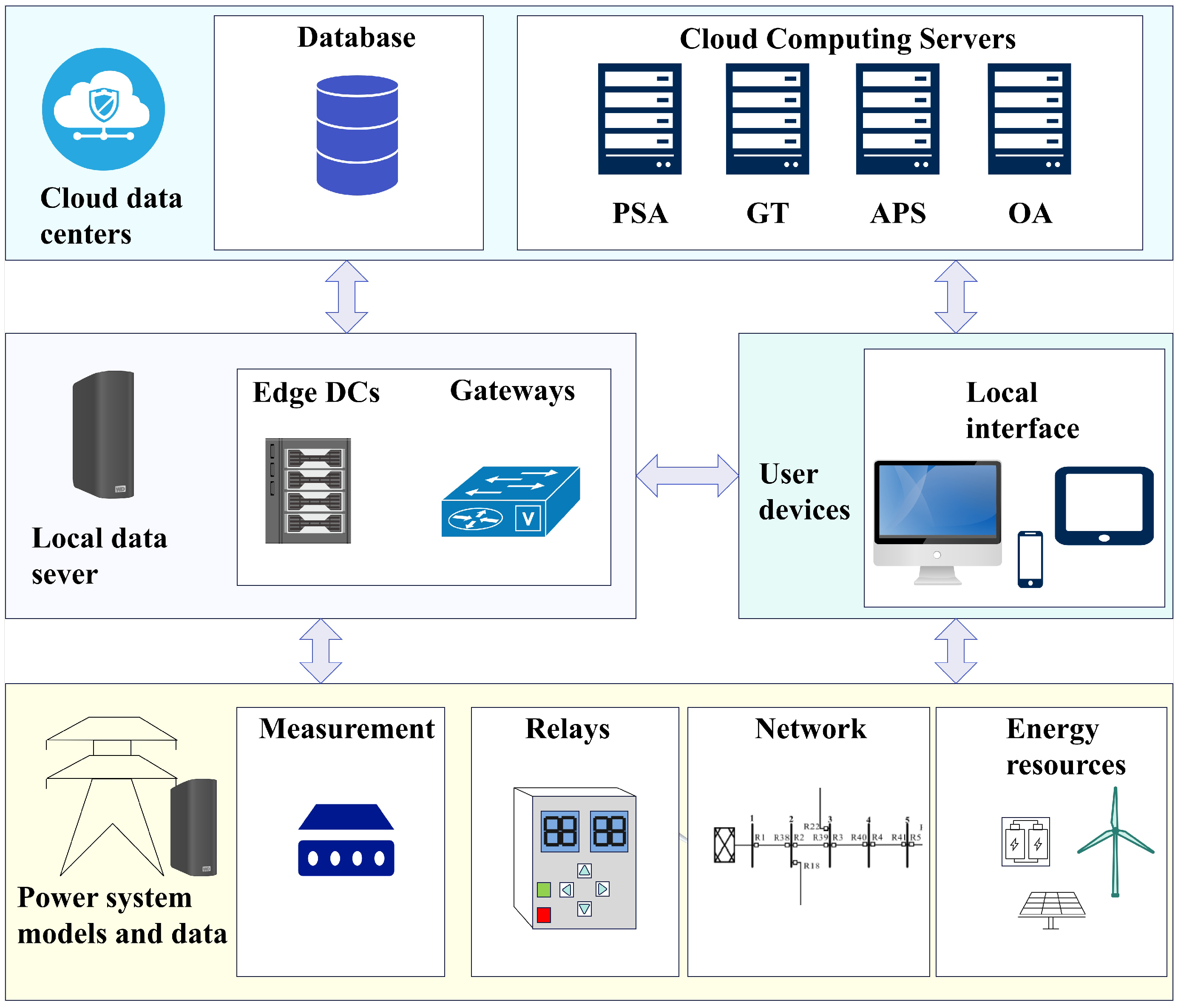
Figure 1 presents an integrated edge computing architecture for the coordination of inverse-time overcurrent protections, which comprises four layers: a cloud data center, local data server, user devices, and power system data and models. The top layer features a centralized cloud infrastructure, including a database and cloud computing server. The database is used to store all information from the system, events, and final configurations of the system. Cloud computing servers were used to perform all system calculations with algorithms related to power system analysis (PSA), graph theory (GT), automatic protection settings (APS), and optimization algorithms (OA) using the CGA, SSA, and PSO. The local data server acts as a hub for data aggregation, pre-processing, and temporary storage. It supports latency-sensitive operations and serves as a fallback node in cloud-disconnected scenarios. This stage is useful for basic local calculations to validate and collect the network data. The user interface layer allows users to consult all the information in the system and the decisions made by the algorithms that coordinate the protection. This layer serves as a crucial interface for users to access comprehensive system information and gain insight into the decision-making processes of the algorithms responsible for coordinating protective measures. In addition, it offers visibility of modifications made to the system, ensuring that users can track changes and understand the evolving state of the protection mechanisms. The layer related to the power system data contains all the information about the test system and the models to be updated. These models and system parameters serve as the foundation for simulating new system changes and updating the settings resulting from all algorithms. In this layer, a comparison of all the algorithms was performed.

The proposed method utilizes a combination of hardware and software resources that support the execution of algorithms, management of databases, and inter-program communication. A principal limitation of the present study is that the final settings of the protection schemes were not physically implemented; instead, the results relied on configuring the protections in software and simulating the correctness of these settings. This limitation will be addressed in future work, in which a microgrid will be incorporated, and the protection settings will be adapted to different system operating conditions. Furthermore, cybersecurity aspects are not considered at this stage, as initial experiments must first be carried out to validate the operational performance of the protection hardware.

2.2. General Procedure

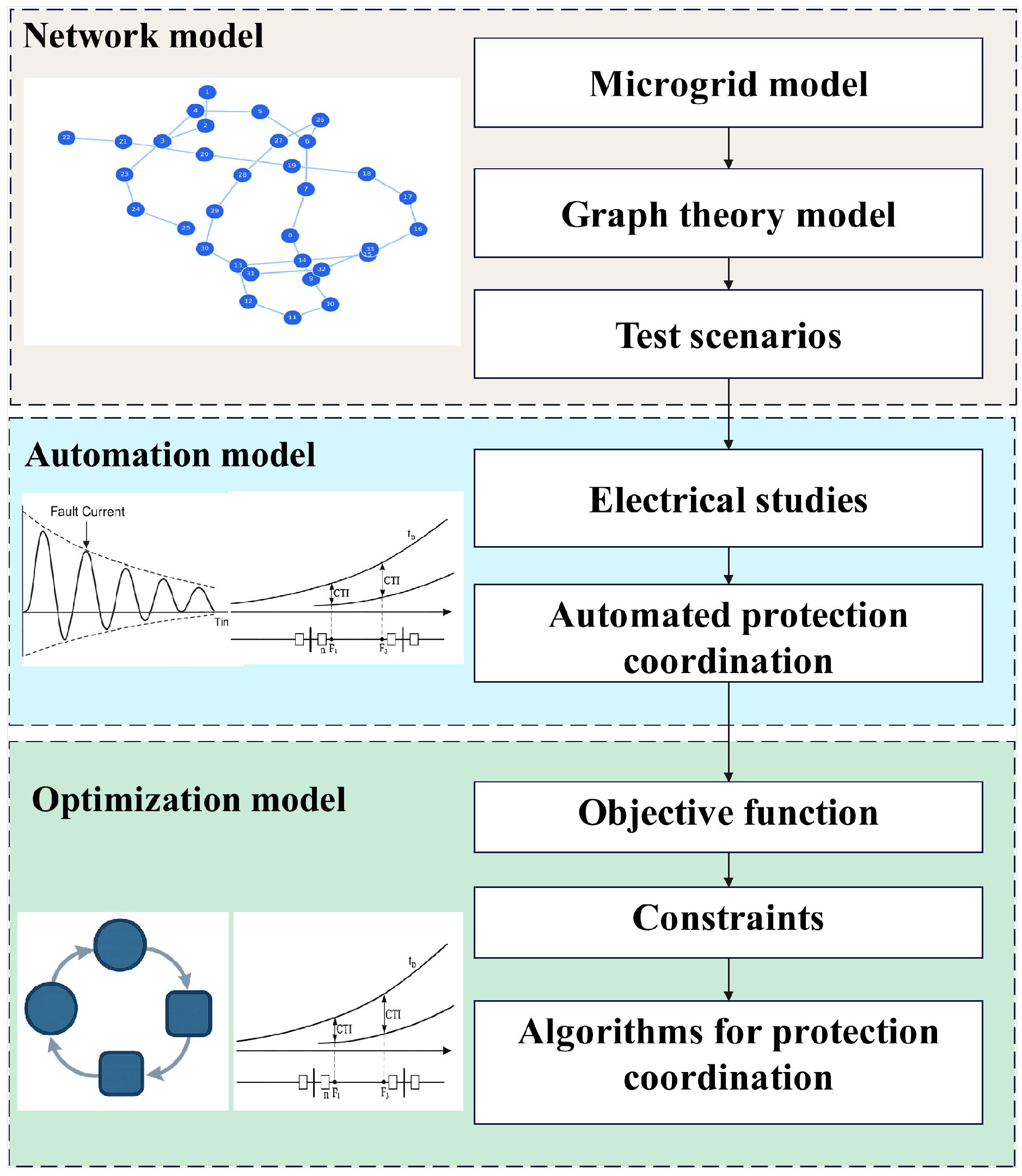
The previous architecture defined the connection of a physical structure. This structure is used to store the general process for conducting all studies. Figure 2 presents the general procedure for implementing optimal inverse-time overcurrent protection in MGs based on edge computing, which consists of three stages to obtain complete mathematical models: network, automation, and optimization.

2.3. Network Model

In this stage, an AC mesh MG was selected and modeled using DIgSILENT PowerFactory 2024 Service Pack 5A. Graph theory is then used to study the network topology and determine the network meshes, fault locations, and relay pairs.

Accurate network models allow for the simulation of various fault scenarios, testing of protection schemes, and optimization of system performance. This stage was designed to represent the MG and different test scenarios were created to perform automated and optimal inverse-time overcurrent relay settings. In this case, two main steps were performed: modeling the MG and defining the test scenarios to evaluate the protection scheme.

2.3.1. MG Model

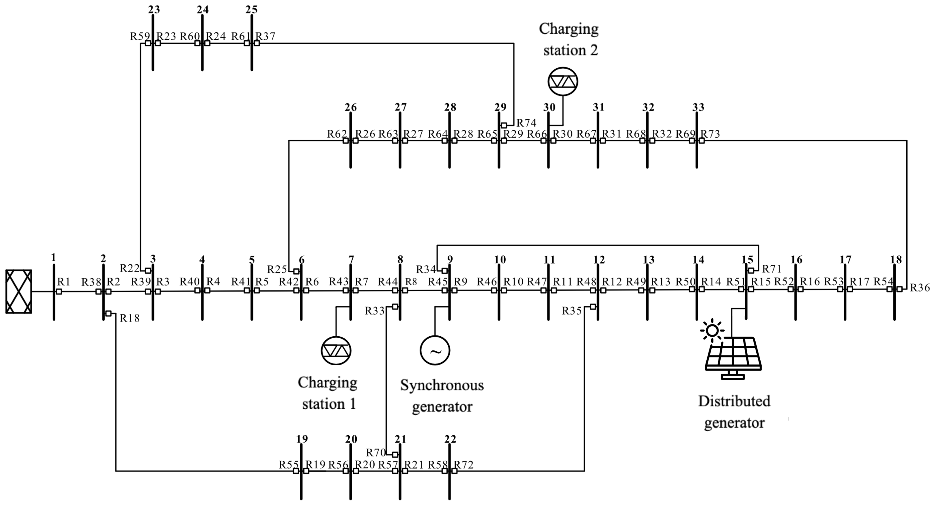
For the study, a modified IEEE 33-bus system configured as a mesh network was used based on the network presented by [15]. The network integrates the DG and EVCS, as shown in Figure 3. For each scenario, a connected topology was activated, represented by graph theory, where the orientation of the segments corresponded to the effective direction of the fault contribution at the point being analyzed.

It is important to recognize that the topology of the fundamental mesh through structural coherence is corroborated by paths delineated from the source to the fault. Inverse-time overcurrent relays are placed to protect the lines and are equipped with a directional unit.

2.3.2. Graph Theory

The analysis of electrical networks can be effectively conceptualized using graph theory. This method can represent a network with nodes that correspond to buses and edges to transmission or distribution lines [17]. This method transforms the physical electrical circuit into a mathematical structure using matrices, such as adjacency and Laplacian matrices, enabling the analysis of network behavior using principles from graph theory and linear algebra [19]. In this method, the adjacency matrix provides a compact representation of the connections between nodes and is defined as follows (Equation (1)).

$$A_{ij}=\left\{\begin{array}{cc}1\hfill & \mathrm{if}\mathrm{there}\mathrm{is}\mathrm{a}\mathrm{line}\mathrm{between}\mathrm{the}\mathrm{nodes}i\mathrm{and}j,\hfill \\ 0\hfill & \mathrm{otherwise},\hfill \end{array}\right.$$

(1)

Fundamental meshes are important for electrical circuit analysis within the framework of graph theory [18]. They represent the basic paths through which current can flow and are useful for power flow analysis and protection coordination. Mathematically, they are defined as a minimal, independent set of cycles that form the basis for all possible cycles in the graph, such that any other cycle can be expressed as a linear combination of these meshes. Their main characteristics are as follows. They are derived from the minimum spanning tree of the graph and calculated using Equation (2). The term e is the number of edges, n is the number of nodes, and $\mu$ is the number of fundamental meshes.

$$\mu =e-n+1,$$

(2)

Line segments are examined to define primary–backup relay relationships by calculating the short-circuit currents at specific fault locations along each line. This graphical representation systematizes the coordination process, ensuring that the relay settings are consistent with the topology and resilient to faults [18]. Multiple operating states are defined by combining the load level, DG availability, and topology changes from the protection operations. For each state, faults were simulated at electrically critical points (segment ends and boundary nodes), and for every relay, the resulting short-circuit and nominal currents were recorded to form the coordination test cases. For each operating scenario s, the active MG is modeled as a connected directed graph according to Equation (3) in which the fault contribution paths are traced.

$${\overrightarrow{G}}_s=\left(\mathcal{N},{\mathcal{E}}_s\right),$$

(3)

In Equation (3), $\mathcal{N}$ is the set of nodes, and ${\mathcal{E}}_s$ is the set of energized segments with their effective orientation. The relay–segment–direction mapping in Equation (4) identifies which relays supervise which segment and in which direction.

$$\psi :\mathcal{R}⟶{\mathcal{E}}_s\times \{\to ,\leftarrow \},\psi \left(r\right)=({\ell }_r,{\mathrm{direction}}_r),$$

(4)

where $\mathcal{R}$ is the set of overcurrent relays. Meanwhile, for a fault f in segment $\ell \in {\mathcal{E}}_s$, the set of contributing sources is ${\mathcal{S}}_{f,s}$. For each source $k\in {\mathcal{S}}_{f,s}$, the oriented path toward the fault is calculated as shown in Equation (5).

$${\mathrm{\Pi }}_{k\to f,s}\subset {\mathcal{E}}_s,$$

(5)

Along the path in Equation (5), the ordered list of relays whose direction corresponds to the flow toward f is extracted, as shown in Equation (6).

$$\mathcal{R}\left({\mathrm{\Pi }}_{k\to f,s}\right)=(r_1,r_2,\dots ,r_q),$$

(6)

Equation (6) generates the primary–backup relay pairs by adjacency, as shown in Equation (7).

$${\mathcal{P}}_{f,k,s}=\{(r_1,r_2),(r_2,r_3),\dots ,(r_{q-1},r_q)\}.$$

(7)

The total set of valid pairs for scenario s is given by Equation (8).

$${\mathcal{P}}_s=\bigcup _f\bigcup _{k\in {\mathcal{S}}_{f,s}}{\mathcal{P}}_{f,k,s}.$$

(8)

2.3.3. Test Scenarios

Table 2. Complete operational scenarios of the modified IEEE 33-node test feeder.

Scenario	Operation Mode		EVCS 1		EVCS 2		Photovoltaic System (DG)
	Grid-Connected	Island	Full Charge	Parcial Discharge	Full Charge	Parcial Discharge
1	✓
2		✓
3		✓					✓
4	✓						✓
5		✓	✓
6		✓		✓
7		✓
8		✓
9		✓			✓
10		✓				✓
11		✓
12		✓
13		✓	✓		✓
14		✓		✓	✓
15		✓	✓			✓
16		✓		✓		✓
17		✓
18		✓
19		✓
20		✓
21	✓		✓
22	✓			✓
23	✓
24	✓
25	✓				✓
26	✓					✓
27	✓
28	✓
29	✓		✓		✓
30	✓			✓	✓
31	✓		✓			✓
32	✓			✓		✓
33	✓
34	✓
35	✓
36	✓
37		✓	✓				✓
38		✓		✓			✓
39		✓					✓
40		✓					✓
41		✓			✓		✓
42		✓				✓	✓
43		✓					✓
44		✓					✓
45		✓	✓		✓		✓
46		✓		✓	✓		✓
47		✓	✓			✓	✓
48		✓		✓		✓	✓
49		✓					✓
50		✓					✓
51		✓					✓
52		✓					✓
53	✓		✓				✓
54	✓			✓			✓
55	✓						✓
56	✓						✓
57	✓				✓		✓
58	✓					✓	✓
59	✓						✓
60	✓						✓
61	✓		✓		✓		✓
62	✓			✓	✓		✓
63	✓		✓			✓	✓
64	✓			✓		✓	✓
65	✓						✓
66	✓						✓
67	✓						✓
68	✓						✓

presents information on the different operating scenarios of the modified IEEE 33-node test feeder, based on the events simulated in [15]. The first column represents the number of simulated scenarios. The second column identifies scenarios in which the operation mode of the MG is considered and divided into two subcolumns: grid-connected and island modes. The third column displays the charging stations, which are divided into two sub-columns: full charge and partial discharge modes. The fourth column considers charging station 2 with two sub-columns: full charge and partial discharge modes. Finally, the fifth column contemplates scenarios in which distributed photovoltaic generators are considered.

Thus, when conducting the entire analysis of the MG, 68 scenarios were considered that combined the mode of operation (grid-connected and island modes), states of electric vehicle charging stations (considering partial and full charging or discharging processes), and the presence or absence of the photovoltaic generation system.

2.4. Automation Model

Figure 4 presents the automation algorithm designed to calculate the protection settings. The algorithm focuses on determining the initial protection settings, obtaining the $TDS$ and the pickup current ($I_{p}i$). A connection between DIgSILENT PowerFactory and Python was performed to run the case scenarios and study the power flow and short circuits. The automatic coordination of protection relays was performed for 68 scenarios and all relay pairs.

2.4.1. Electrical Studies

To obtain the data required for protection coordination, two studies were automatically performed: power-flow and short-circuit analyses. The power flow is useful for determining the voltage magnitudes and angles, currents, and powers in all branches of the network. Short-circuit analysis is used to obtain the currents experienced by system elements, such as lines, transformers, DG, and the main electrical grid. The study was conducted for 68 scenarios that considered connection modes and generator operation. Faults were simulated for each line to evaluate the most critical selectivity events, and currents were recorded for each protection device.

2.4.2. Automated Coordination

The initial values are computed for each relay: pickup $I_{pi}$ and $\mathrm{TDS}$. As a practical rule, $I_{pi}$ is set above the rated current to avoid load tripping (e.g., $I_{pi}=1.25I_{\mathrm{nom}}$). $\mathrm{TDS}$ is selected to satisfy the minimum coordination interval $CT{I}_{min}$ (typically $\ge 0.2$ s). Finally, it is validated that $I_{pi}$ preserves both sensitivity and security, the $CTI$ margins are respected, the clearing times are compatible with requirements, and all variables remain within the limits of the manufacturer.

The TDS is responsible for regulating the response speed of a relay under overcurrent conditions, according to an inverse time characteristic established by the IEC 60255-151 standard [20]. In this study, a standard inverse time relay (SI) was adopted, whose operating curve was defined by the constants $k=0.14$ and $n=0.02$, as specified in the IEC 60255-151 standard and validated in previous studies [20,21]. These values ensure a moderately inverse response, allowing the operating time to decrease as the fault current increases, which facilitates coordination in networks under variable conditions [15]. The operating time ($t_i$) was determined using the following expression:

$$t_i={\displaystyle \frac{k}{{\left(\frac{I_{shc}}{I_{pi}}\right)}^n-1}}\times TD{S}_i$$

(9)

The term $t_i$ is the relay operation time i (in seconds), $I_{shc}$ is the short-circuit current in front of the relay, $I_{pi}$ is the pickup current adjusted in the relay i, k and n are constants of the SI curve, and $TD{S}_i$ is the time adjusted in the relay i.

The proper selection of the TDS is crucial to ensure that the backup relays operate after the main protection relays, maintaining a typical CTI (0.2–0.5 s), and avoiding compromising the stability of the system [22,23].

The pickup current ($I_{pi}$) establishes the umbral of relay activation and is calculated as follows:

$$I_{pi}=1.25·I_{nom}$$

(10)

The term $I_{nom}$ represents the nominal current of the load. This factor of 1.25 provides a margin for transient conditions, reducing unnecessary trips and ensuring that the relay operates only in the event of sustained faults [24]. In MGs with DG, $I_{pi}$ may require dynamic adjustments due to fluctuations in $I_{nom}$ depending on the topology and operating mode [25].

The effectiveness of coordination between overcurrent relays is fundamental to avoiding miscoordination that could compromise the stability of MGs, particularly in mesh network topologies with DG. In this regard, Ghadiri and Mazlumi [15] proposed specific indices to assess the coordination performance between pairs of primary and backup relays: miscoordination time ($\Delta t_{mbj}$), individual miscoordination time (MT), and total miscoordination time (TMT). These indices enable the quantification and analysis of selectivity failures, which are critical aspects of networks with variable fault currents [25,26].

The miscoordination time for the j-th pair of primary–backup relays is defined as

$$\Delta t_{mbj}=t_{bj}-t_{mj}-CTI$$

(11)

where $t_{mj}$ is the operating time of the main relay, $t_{bj}$ is the operating time of the backup relay, and $CTI$ is the coordination time interval, which is typically between 0.2 s and 0.5 s. A positive value of $\Delta t_{mbj}$ indicates proper coordination (the backup relay operates after the main relay with the required margin), whereas a negative value indicates a lack of coordination, as the backup relay operates sooner than desired [15].

The individual miscoordination time index ($M{T}_j$) measures the magnitude of miscoordination for each pair of relays and is calculated as

$$M{T}_j={\displaystyle \frac{\Delta t_{mbj}-|\Delta t_{mbj}|}{2}}$$

(12)

This index is always negative or zero. If $\Delta t_{mbj}>0$ (correct coordination), $M{T}_j=0$; if $\Delta t_{mbj}<0$ (lack of coordination), $M{T}_j$ takes a negative value whose magnitude increases with the degree of miscoordination, reflecting a deterioration in the selectivity of the j-th pair [15].

To evaluate the overall coordination in a specific operational scenario, the total discoordination time index ($TM{T}_{Scn}$) is introduced for the n-th scenario ($S{c}_n$), expressed as

$$TM{T}_{Scn}=\sum _{j=1}^{k}M{T}_j$$

(13)

where k is the number of relay pairs in scenario $S{c}_n$. Similar to $M{T}_j$, $TM{T}_{Scn}$ is negative or zero, and a more negative value indicates greater accumulated miscoordination between the relay pairs. Coordination improves when the absolute value of $TM{T}_{Scn}$ decreases and approaches zero ($TM{T}_{Scn}\to 0^{-}$), reflecting a reduction in miscoordination and greater selectivity in the system [15].

These indices are particularly useful for MGs with DG, where fluctuations in fault currents can worsen miscoordination. A high $TM{T}_{Scn}$ value can allow faults to propagate, thereby increasing the risk of cascading failures. Therefore, detailed analyses and simulations are required to optimize the relay settings, minimize $TM{T}_{Scn}$ and ensure reliable protection [15].

2.5. Optimization Model

The protection settings obtained in the previous phase ensured feasibility but did not maximize the response speed or minimize miscoordination. Consequently, this stage recalculates the parameters $I_{pi}$ and $TDS$ using an optimization technique for nonlinear problems with multiple constraints and high dimensionality [23,26]. The optimization stage involves designing a mathematical model to minimize the TMT. Three metaheuristic algorithms (CGA, SSA, and PSO) were used to improve the performance and decision-making process.

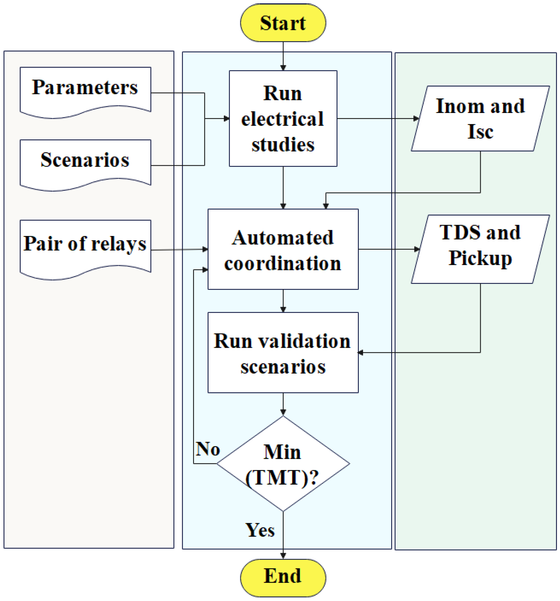
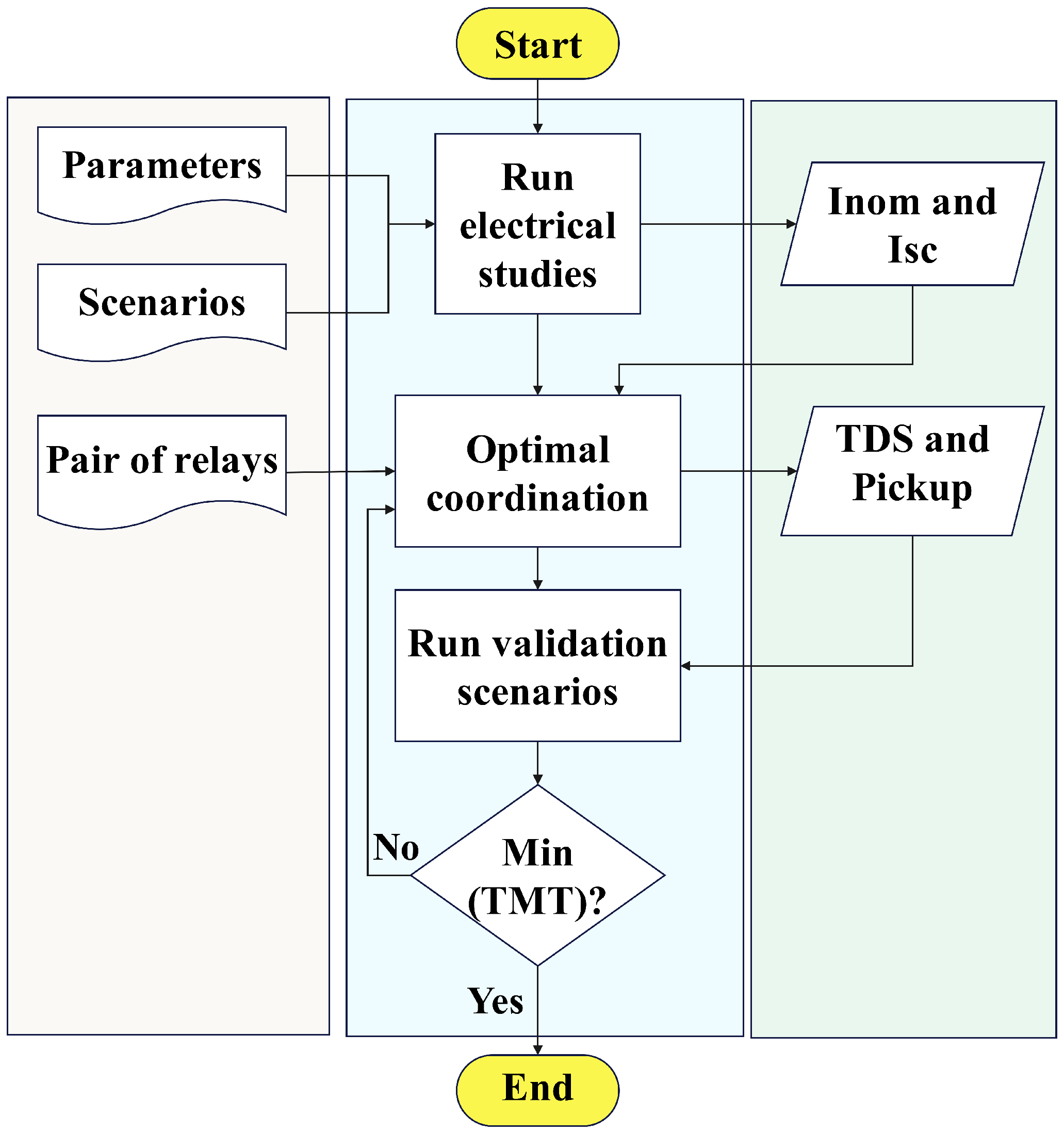
Figure 5 outlines the sequential methodology for achieving optimal relay coordination through electrical analysis and iterative validation. The process begins with the input of system parameters, fault scenarios, and relay pair configurations. Electrical simulations were conducted to determine the nominal operating current ($I_{nom}$) and short-circuit current ($I_{sc}$), which served as the basis for calculating coordination settings. The optimal coordination stage computes the TDS and pickup currents ($I_{pi}$) for each relay to satisfy the protection selectivity and timing constraints. These settings were then evaluated through validation scenarios to assess their effectiveness under varying fault conditions. A decision node checks whether the minimum TMS is achieved. If the condition is not met, the process loops back to refine the coordination parameters. Once the convergence criteria are satisfied, the algorithm terminates, ensuring that the relay settings meet the desired coordination objectives.

2.5.1. Objective Function

The objective function for the optimization is defined in Equation (14). This function corresponds to minimizing fault-clearing times to maintain selectivity. The objective function sums the times of the relay pairs and penalizes constraint violations.

$$\begin{array}{c}\underset{\mathbf{x}}{min}J\left(\mathbf{x}\right)=\sum _{s\in \mathcal{S}}\sum _{f\in \mathcal{F}}\sum _{r\in \mathcal{R}}{w}_r{t}_{r,f,s}\left(\mathbf{x}\right)+\cdots \\ \lambda \sum _{s\in \mathcal{S}}\sum _{f\in \mathcal{F}}\sum _{(r,b)\in {\mathcal{P}}_s}{\left[CT{I}_{min}-\Delta t_{(r\to b),f,s}\left(\mathbf{x}\right)\right]}_{+}\end{array}$$

(14)

where ${\left[z\right]}_{+}=max(0,z)$ and $w_r$ weighs the relative criticality. For extreme robustness, the min–max variant (15) can be used.

$$\begin{array}{c}\underset{\mathbf{x}}{min}\underset{s\in \mathcal{S}}{max}{\mathrm{\Phi }}_s\left(\mathbf{x}\right)\\ {\mathrm{\Phi }}_s\left(\mathbf{x}\right)=\sum _{f\in \mathcal{F}}\sum _{r\in \mathcal{R}}{w}_r{t}_{r,f,s}\left(\mathbf{x}\right)+\cdots \\ \lambda \sum _{(r,b)\in {\mathcal{P}}_s}\sum _{f\in \mathcal{F}}{\left[CT{I}_{min}-\Delta t_{(r\to b),f,s}\left(\mathbf{x}\right)\right]}_{+}\end{array}$$

(15)

2.5.2. Constraints

The decision variables are expressed in a vector containing the pickup current and time dial of each relay, as expressed in Equations (16) and (17).

$$\mathbf{x}={\left((I_{pi,r},{\mathrm{TDS}}_r)\right)}_{r\in \mathcal{R}},$$

(16)

$$\mathbf{x}={\left(I_{pi,1},{\mathrm{TDS}}_1,I_{pi,2},{\mathrm{TDS}}_2,\dots ,I_{pi,R},{\mathrm{TDS}}_R\right)}^{\top }.$$

(17)

As input data, we consider $I_{r,f,s}^{\mathrm{sc}}$ (short-circuit current seen by each relay), $I_{r,s}^{\mathrm{nom}}$ (rated current), bounds $\left[I_{pi,r}^{min},I_{pi,r}^{max}\right]$ and $\left[{\mathrm{TDS}}_r^{min},{\mathrm{TDS}}_r^{max}\right]$, and the coordination margin $CT{I}_{min}$.

The trip time of relay r for fault f in scenario s is modeled using the IEC family (18).

$$t_{r,f,s}\left(\mathbf{x}\right)={\mathrm{TDS}}_r{\displaystyle \frac{K}{{\left({\displaystyle \frac{I_{r,f,s}^{\mathrm{sc}}}{I_{pi,r}}}\right)}^{\alpha }-1}}+t_r^{\mathrm{add}},$$

(18)

The terms K and $\alpha$ depend on the selected IEC curve, and $t_r^{\mathrm{add}}$ accounts for additional delays, if applicable. Using these times, the primary–backup margin is obtained using Equation (19).

$$\Delta t_{(r\to b),f,s}\left(\mathbf{x}\right)=t_{b,f,s}\left(\mathbf{x}\right)-t_{r,f,s}\left(\mathbf{x}\right).$$

(19)

To employ the IEC–SI curve reported in the literature, the parameters $K=0.14$ and $\alpha =0.02$ (standard inverse form) were used in Equation (18).

2.5.3. Feasibility Constraints

The settings must respect the limits of the equipment according to Equation (20), and simultaneously, the safety and sensitivity of the pickup current are obtained considering Equation (21).

$$\begin{array}{c}{I}_{pi,r}^{min}\le I_{pi,r}\le I_{pi,r}^{max}\\ {\mathrm{TDS}}_r^{min}\le {\mathrm{TDS}}_r\le {\mathrm{TDS}}_r^{max}\\ \forall r\in \mathcal{R}\end{array}$$

(20)

$$\begin{array}{c}{I}_{pi,r}\ge k_{\mathrm{seg}}\underset{s\in \mathcal{S}}{max}{I}_{r,s}^{\mathrm{nom}}\\ I_{pi,r}\le k_{\mathrm{sen}}\\ \underset{(f,s)\in \mathcal{F}\times \mathcal{S}}{min}{I}_{r,f,s}^{\mathrm{sc}}\end{array}$$

(21)

To reflect the practical rule $I_{pi}=1.25I_{\mathrm{nom}}$, Equation (21) can be specialized by considering $k_{\mathrm{seg}}=1.25$ in Equation (21), while maintaining the upper sensitivity limit.

$$I_{pi,r}=1.25\underset{s\in \mathcal{S}}{max}{I}_{r,s}^{\mathrm{nom}},$$

(22)

The operational implementation of the selectivity for all relay pairs, faults, and scenarios is expressed in Equation (23), which is obtained using times from Equation (18).

$$\begin{array}{c}\Delta t_{(r\to b),f,s}\left(\mathbf{x}\right)\ge CT{I}_{min}\\ \forall (r,b)\in {\mathcal{P}}_s,\forall f\in \mathcal{F},\forall s\in \mathcal{S}\end{array}$$

(23)

2.5.4. Miscoordination Index

With the margin expressed in Equation (19), the slack with respect to the CTI required in Equation (23) is defined in Equation (24):

$$\Delta t_{(m\to b),f,s}^{\mathrm{req}}=\Delta t_{(m\to b),f,s}\left(\mathbf{x}\right)-CT{I}_{min}.$$

(24)

The individual miscoordination index is given by Equation (25) and becomes zero when the coordination is maintained.

$$M{T}_{(m,b),f,s}={\displaystyle \frac{\Delta t_{(m\to b),f,s}^{\mathrm{req}}-|\Delta t_{(m\to b),f,s}^{\mathrm{req}}|}{2}}.$$

(25)

The total miscoordination of scenario s is accumulated as shown in Equation (26).

$$TM{T}_s=\sum _{(m,b)\in {\mathcal{P}}_s}\sum _{f\in \mathcal{F}}M{T}_{(m,b),f,s}.$$

(26)

The penalty in Equation (14) based on ${[CT{I}_{min}-\Delta t]}_{+}$ is equivalent (up to scaling) to penalizing $-MT$ in Equation (25), so Equation (14) already captures $TM{T}_s$.

2.5.5. Optimization Algorithms

The optimization problem defined above is regarded as nonlinear and nonconvex. Therefore, it was addressed using optimization algorithms capable of exploring complex feasible regions and handling constraints using penalty-based formulations. In this study, three algorithms are considered: the Continuous Genetic Algorithm (CGA), Salp Swarm Algorithm (SSA), and Particle Swarm Optimization (PSO). These algorithms were selected because they have been extensively used to solve engineering problems in different areas related to renewable energy systems and microgrids (MGs) [27,28,29]. All three adopt the same encoding, evaluation scheme, and termination criteria; the difference is concentrated in the update rule used to generate new candidates within the search space. Accordingly, each individual, particle, or salp is encoded as a candidate configuration for the optimal coordination of relay pairs in each test scenario, that is, a decision vector that groups $I_{pi}$ and $TDS$ for all relay pairs. The initial population is generated through uniform sampling within the admissible bounds (20) and (21); however, to accelerate convergence without compromising feasibility, $I_{pi}$ is initialized to approximately 1.25 $I^{nom}$ (consistent with (22)), and $I_{pi}^{max}$ is restricted to a fraction of the minimum short-circuit current observed across scenarios and fault locations. This prevents the search from carrying out evaluations in regions where selectivity cannot be achieved or where the resulting settings tend to cause undesired tripping under the load conditions.

Under this representation, the differences among the algorithms are concentrated in the rules they use to update the population, that is, in how they generate and replace candidate solutions. In the case of the CGA, new individuals are obtained by randomly selecting two parents and applying a one-point crossover to recombine segments of the decision vector. Population diversity is preserved through sparse mutation, which re-samples within the bounds of a reduced number of genes per individual, denoted $n_{mut}$. After evaluating the offspring using (14), an elitist replacement is applied: if an offspring improves upon the worst individual and is not a duplicate, it replaces it while always preserving the best solution found [30]. In the SSA, neither crossover nor mutation operators are used. The population is organized as a chain with a leader and followers: the leader moves guided by the best global solution, whereas the followers are updated with respect to the preceding individual. This behavior is particularly useful when tuning the continuous variables $I_{pi}$ and $TDS$, as it reduces abrupt perturbations that may degrade the coordination margins of the relay pairs [31]. In PSO, each candidate incorporates dynamic memory through a velocity associated with its position. At each iteration, the particles combine inertia from the previous motion with an attraction toward their best historical position, referred to as the cognitive component, and the swarm’s global best solution, referred to as the social component. This often leads to fast convergence once the coordinated regions emerge, while still retaining the ability to escape local minima owing to the swarm diversity and the interaction between the individual memory and collective guidance [32].

Notably, regardless of the algorithm employed in this methodology, all algorithms share the same constraint-handling strategy. After each update, a bound-control step is applied to ensure that the variables remain within the defined search area. Subsequently, each candidate solution is evaluated through the objective function, promoting feasibility via penalty terms associated with constraint violations and operating times that exceed the implicit operational limit. As a result, the best solutions are preserved under an explicit elitist scheme in the CGA and under the global-best mechanism inherent to SSA and PSO, thereby preventing deterioration in fitness or regression away from globally optimal solutions.

Once the settings are determined, the operating times are recomputed using Equation (18), and the global selectivity is audited using Equations (19)–(23) for all faults and scenarios considered. As a closing step, the fraction of coordinated pairs is reported, and $TM{T}_s$ is computed for each scenario according to Equation (26). In addition, compliance with the bounds in Equation (20) is verified, together with adherence to the threshold $t_{max}$. To ensure traceability and reproducibility, the final settings were logged along with the scenario identifier and generation date, and the t–I curves of the most critical pairs were included to document compliance with the temporal coordination margin.

3. Results

This section presents the results organized into five subsections: graph theory applied to MG, automation of protection settings, optimization of protection settings, and a comparison of the inverse-time overcurrent protection curves of the proposed methods.

3.1. Graph Theory Applied to the MG

As described in the methods, graph theory was applied in this study to identify nodes, topology, critical fault points, and optimize protection coordination. Therefore, the approach involves using adjacency matrices to find the fundamental meshes that transform the circuits into mathematical structures for analysis.

3.1.1. Adjacency Matrix

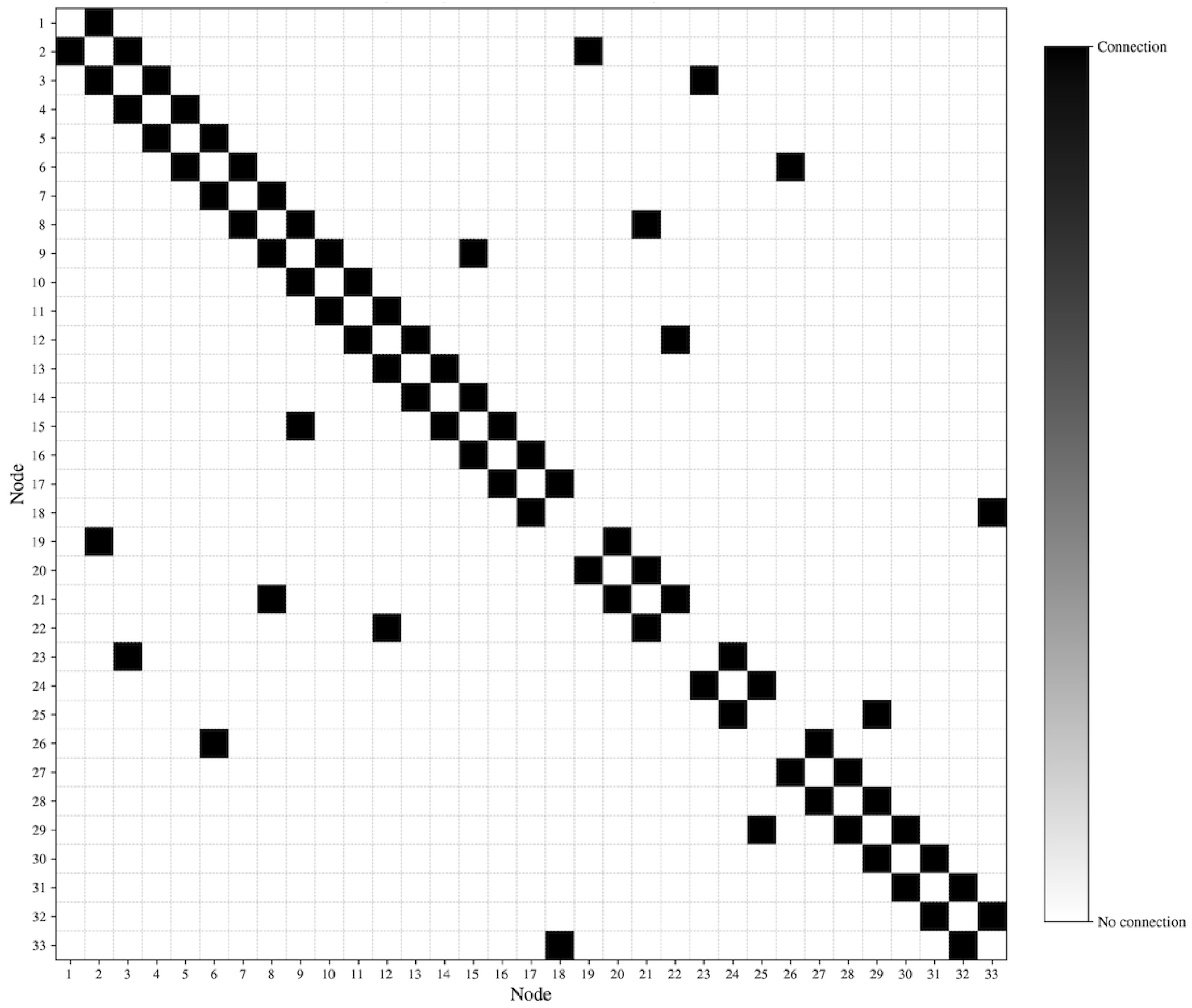
Figure 6 shows an adjacency matrix that represents the topological connectivity of the entire MG. Each cell in the matrix corresponds to a potential connection between the two nodes. Each cell represents the existence or absence of a direct connection between two nodes: black squares indicate an active connection, and white squares denote the absence of a link. The main diagonal in black reflects self-connections. This matrix allows for a clear and concise visualization of the network topology, facilitating connectivity analysis, critical node identification, and zone-based clustering detection. Moreover, its symmetrical structure suggests that the connections are in meshes and the way in which they can be represented for the bidirectional study of electrical protection.

3.1.2. Fundamental Meshes

Table 3. Fundamental meshes identified in the MG with their respective paths.

Mesh	Path
Mesh 1	1–2–3–4–5–6–7–8–9–10–11–12–13–14–15–16–17–18–33–32–31–30–29–25–24–23–3–2–1
Mesh 2	1–2–3–4–5–6–26–27–28–29–25–24–23–3–2–1
Mesh 3	1–2–19–20–21–22–12–13–14–15–16–17–18–33–32–31–30–29–25–24–23–3–2–1
Mesh 4	1–2–3–4–5–6–7–8–21–22–12–13–14–15–16–17–18–33–32–31–30–29–25–24–23–3–2–1
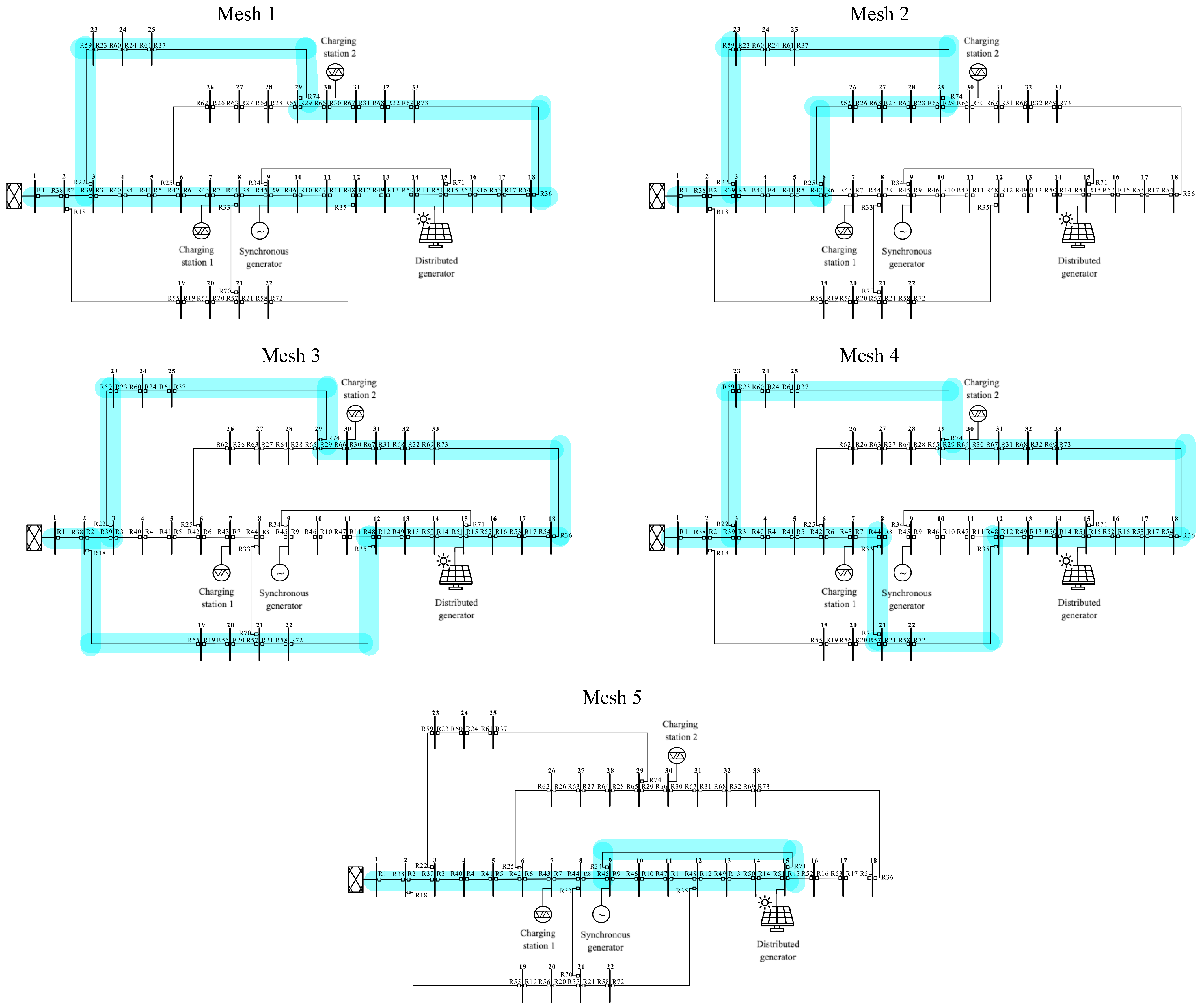
Mesh 5	1–2–3–4–5–6–7–8–9–10–11–12–13–14–15–9–8–7–6–5–4–3–2–1

presents the fundamental meshes identified in the topology of the MG under study, along with their respective nodes. Each mesh represents an independent loop within the system, which is useful for analyzing power flows, fault currents, and protection studies. These meshes were determined by a topological analysis of the MG graph, ensuring linear independence between the paths and complete coverage of the system. Their identification is essential for the formulation of mesh equations in circuit analysis studies, contingency simulations, and protection scheme designs. The enumeration of nodes follows a logical sequence that reflects the physical connectivity between the system elements. Mesh 1 shows a complete path that encompasses all the main nodes of the system, forming a closed loop from node 1 to node 27 and returning to node 1. This mesh represents the external contours of the MG. Mesh 2 includes the nodes of the central segment and part of the left loop, highlighting the interaction between nodes 3 and 30 and its return through node 23 to node 1. Mesh 3 represents an extended version of Mesh 2, incorporating additional nodes from the right loop and closing the path through Node 27. Mesh 4 considers the entire perimeter of the system, including all nodes from 1 to 27, allowing the evaluation of the redundancy and protection coverage in the network. Mesh 5 represents an internal loop connecting the central and peripheral nodes, with an emphasis on nodes 6 to 19, and a return through nodes 7 and 3 to node 1.

Figure 7 presents the fundamental meshes identified in the modified IEEE 33-node test feeder, which was used for the topological analysis of the MG. Each subfigure highlights the path corresponding to an independent mesh in the distribution network. These meshes were selected based on the criteria of linear independence and structural coverage, allowing the formulation of equations for load flow studies, fault detection, and protection identification. The representation considers the points where all the elements are located, such as buses, switches, DG, and distribution lines, facilitating the visualization of the connectivity of the MG. This automation eliminates slow and manual processes required to identify the loops, making it highly practical for complex topologies of MGs that are continually changing.

3.1.3. Protection

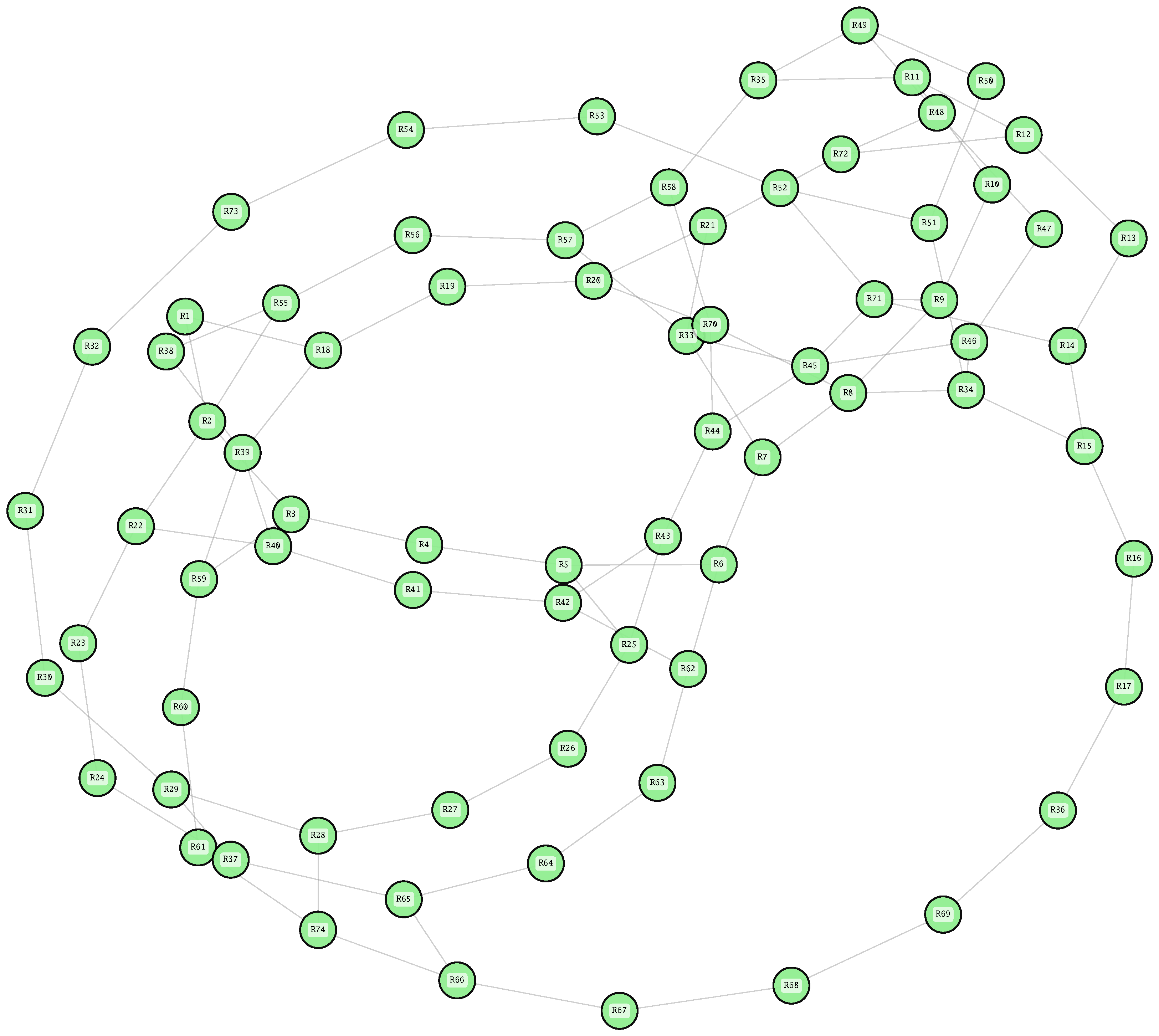
Figure 8 illustrates a diagram of the closest relations of each protection relay. Each node of the graph represents a relay, and each edge indicates that both devices share at least one primary–backup relay pair. All relays have at least one connection; however, those with a higher degree (R8, R2, R33, R39, and R70) are critical, as a change in their parameters affects several protection routes. The diagram provides information about multiple protection routes that automation processes and engineers must consider when calculating settings and avoid miscoordination. This allows protection engineers to quickly understand the dependency structure of the network, which is essential for both manual and automated coordination strategies. In addition, an operator can immediately see which other relay zones are affected, providing the structural data required to formulate the coordination constraints for the entire system.

Table 4. Relay pairs related to each line of the MG.

#	Line	Relay Pair	#	Line	Relay Pairs
1	L1–2	R38, R39	51	L25–29	R74, R28
2	L1–2	R38, R55	52	L25–29	R74, R66
3	L10–11	R47, R48	53	L25–29	R37, R24
4	L10–11	R10, R9	54	L26–27	R63, R64
5	L11–12	R48, R49	55	L26–27	R26, R25
6	L11–12	R48, R72	56	L27–28	R64, R65
7	L11–12	R11, R10	57	L27–28	R27, R26
8	L12–13	R49, R50	58	L28–29	R65, R37
9	L12–13	R12, R11	59	L28–29	R65, R66
10	L12–13	R12, R72	60	L28–29	R28, R27
11	L13–14	R50, R51	61	L29–30	R66, R67
12	L13–14	R13, R12	62	L29–30	R29, R28
13	L14–15	R51, R52	63	L29–30	R29, R37
14	L14–15	R51, R34	64	L3–23	R59, R60
15	L14–15	R14, R13	65	L3–23	R22, R2
16	L15–16	R52, R53	66	L3–23	R22, R40
17	L15–16	R15, R14	67	L3–4	R40, R41
18	L15–16	R15, R34	68	L3–4	R3, R2
19	L16–17	R53, R54	69	L3–4	R3, R59
20	L16–17	R16, R15	70	L30–31	R67, R68
21	L17–18	R54, R73	71	L30–31	R30, R29
22	L17–18	R17, R16	72	L31–32	R68, R69
23	L18–33	R73, R32	73	L31–32	R31, R30
24	L18–33	R36, R17	74	L32–33	R69, R36
25	L19–20	R56, R57	75	L32–33	R32, R31
26	L19–20	R19, R18	76	L4–5	R41, R42
27	L2–19	R55, R56	77	L4–5	R4, R3
28	L2–19	R18, R1	78	L5–6	R42, R43
29	L2–19	R18, R39	79	L5–6	R42, R62
30	L2–3	R39, R40	80	L5–6	R5, R4
31	L2–3	R39, R59	81	L6–26	R62, R63
32	L2–3	R2, R1	82	L6–26	R25, R5
33	L2–3	R2, R55	83	L6–26	R25, R43
34	L20–21	R57, R58	84	L6–7	R43, R44
35	L20–21	R57, R33	85	L6–7	R6, R5
36	L20–21	R20, R19	86	L6–7	R6, R62
37	L21–22	R58, R35	87	L7–8	R44, R70
38	L21–22	R21, R20	88	L7–8	R44, R45
39	L21–22	R21, R33	89	L7–8	R7, R6
40	L8–21	R70, R58	90	L8–9	R45, R46
41	L8–21	R70, R20	91	L8–9	R45, R71
42	L8–21	R33, R7	92	L8–9	R8, R7
43	L8–21	R33, R45	93	L8–9	R8, R70
44	L12–22	R35, R11	94	L9–10	R46, R47
45	L12–22	R35, R49	95	L9–10	R9, R8
46	L12–22	R72, R21	96	L9–10	R9, R71
47	L23–24	R60, R61	97	L9–15	R71, R14
48	L23–24	R23, R22	98	L9–15	R71, R52
49	L24–25	R61, R74	99	L9–15	R34, R8
50	L24–25	R24, R23	100	L9–15	R34, R46

presents the relationship between each relay pair identified in the graph with the lines of the MG. The first column presents the number of relay pairs in the system, the second column shows the lines, and the third column displays the relay pairs. The table shows a total of 100 relay pairs identified in the network. In this relation, at least one of the relays is located in the same line, and the other is located in the following lines of the network. This result is used to detect the current measured for the relay pairs when a fault occurs at each line. After determining the corresponding currents, the coordination of the relay pairs can be performed.

3.2. Automation of Protection Settings

Within the automation process, 6800 relay pairs were directly processed and grouped into 68 different scenarios for the protection system. For each pair, the coordination time margin was calculated using the mathematical model defined in Section 2, where a relay pair is considered coordinated if $\Delta t\ge 0$; otherwise, a violation of the time margin is identified. In addition, the coordination percentage of each scenario was estimated as the fraction of pairs with $\Delta t\ge 0$, along with descriptive statistics of $\Delta t$ (mean, standard deviation, minimum, and maximum).

Table 5. Global statistical summary of the 68 scenarios (direct calculation from the original source).

Indicator	Value
Total scenarios	68
Mean TMT	$-17.875\mathrm{s}$
Minimum TMT	$-45.681\mathrm{s}$
Maximum TMT	$-14.815\mathrm{s}$
Median TMT	$-16.757\mathrm{s}$
Mean coordination	$12.2\%$
Minimum coordination	$7.0\%$
Maximum coordination	$16.0\%$
Pairs per scenario (mean/min/max)	$100.0/100/100$

summarizes the results obtained for the 68 scenarios. It shows that the sample size per scenario and the baseline performance exhibit accumulated incoordination: the average $\mathrm{TMT}$ is negative, and its dispersion, measured by the range between the minimum and maximum, confirms the presence of severe scenarios. The average coordination is low, indicating that the fraction of pairs that meet $\Delta t\ge 0$ is small. This reading, supported by the distribution of the $\mathrm{TMT}$ sign, establishes the starting point for the protection scheme without adjustments and requires actions aimed at shifting $\mathrm{TMT}\to 0$ and substantially increasing the compliance coverage.

Table 6. TMT by scenario based on original data in two-panel format (The left half lists from the most severe case and the right half continues in the same order).

Scenario	TMT (s)	Coord. (%)	Scenario	TMT (s)	Coord. (%)
14	−45.681	14	21	−15.992	12
15	−32.153	14	22	−15.895	12
5	−24.948	13	27	−15.877	13
16	−23.647	11	31	−15.867	11
45	−22.857	13	1	−15.854	12
46	−2151	12	28	−15.843	12
6	−20.975	13	26	−15.809	7
47	−20.795	12	32	−15.805	11
9	−20.147	14	29	−15.727	15
48	−19.980	10	25	−15.696	12
37	−19.964	10	36	−15.695	10
38	−19.490	8	23	−15.690	10
10	−19.227	14	30	−15.688	9
8	−19.003	12	34	−15.668	11
2	−18.962	12	24	−15.590	15
41	−18.764	14	35	−15.567	11
13	−18.450	13	33	−15.541	12
18	−18.325	10	53	−15.508	9
20	−18.232	11	63	−15.476	15
12	−18.117	11	61	−15.426	11
19	−18.061	13	54	−15.375	13
39	−17.967	13	64	−15.363	11
40	−17.840	13	62	−15.331	14
3	−17.822	13	57	−15.263	12
11	−17.813	12	58	−15.259	12
7	−17.786	14	4	−15.231	13
50	−17.786	9	59	−15.162	12
17	−17.773	13	55	−15.091	15
49	−17.756	11	60	−15.058	12
42	−17.731	16	68	−15.043	16
52	−17.647	13	56	−14.987	12
44	−17.643	10	66	−14.945	14
51	−17.583	14	67	−14.898	14
43	−17.522	13	65	−14.815	15

breaks down the diagnosis at the scenario level and enables technical prioritization of the results. The $\mathrm{TMT}$ captures the accumulated severity of CTI violations in each case, whereas the coordination column expresses the proportion of relay pairs that satisfy $\Delta t\ge 0$. The average $\overline{\Delta t}$ and the total number of relay pairs contextualize the magnitude and bias of the time margins. The combination of a more negative $\mathrm{TMT}$ with relatively low coordination identifies critical hotspots that should be addressed first by time adjustments and curves, verification of CTI assumptions, and a review of the representative failure conditions. It is important to note that $\overline{\Delta t}$ can be positive in scenarios where both positive and negative margins coexist, but a negative $\mathrm{TMT}$ indicates that violations persist that degrade selectivity. Therefore, the joint reading of $\mathrm{TMT}$ and coordination is an effective guide for prioritizing intervention and measuring the impact of improvements in the before-and-after comparison.

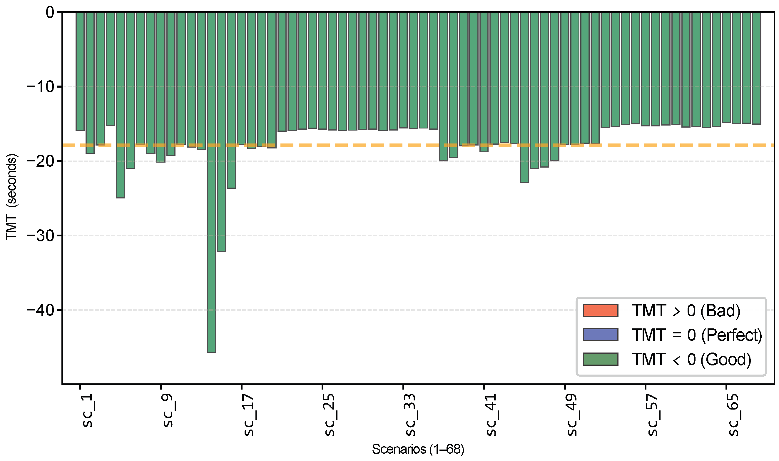
Figure 9 presents the graph of the TMT obtained for the scenarios. The graph shows green bars, or TMT with values less than zero, which indicates that good protection coordination was achieved. In addition, no red bars were observed in this figure, which would correspond to TMT greater than zero or bad values. Furthermore, no TMT with values equal to zero (blue) were found, indicating that perfect protection coordination was not achieved. Moreover, the average value of TMT is plotted with a yellow dotted line.

3.3. Optimal Protection Settings

Within the previously implemented automation process, several relay pairs remained uncoordinated. Therefore, it is important to incorporate new methodologies, such as optimization algorithms, which can enable the optimal coordination of protection settings. Accordingly, this study adopts different optimization techniques that are widely reported in the specialized literature, namely CGA, PSO, and SSA.

It is important to note that this methodology is implemented online through edge computing, which ensures that the validation is carried out across all test scenarios available in the database, as diagnosing the coordination of relay pairs in the MG under the full set of possible operating conditions is essential. Accordingly,

Table 7. Coordination status and minimum values of TDS and pickup for CGA, PSO, SSA, and SCA.

Scenario ID	CGA			PSO			SSA
	Status	Min TDS	Min Pickup	Status	Min TDS	Min Pickup	Status	Min TDS	Min Pickup
1	✓	0.141	0.062	✓	0.324	0.099	✓	0.206	0.058
2	✓	0.099	0.027	✓	0.293	0.013	✓	0.144	0.032
3	✓	0.132	0.017	✓	0.333	0.019	✓	0.206	0.019
4	✓	0.088	0.07	✓	0.305	0.103	✓	0.242	0.088
5	✓	0.115	0.016	✓	0.306	0.04	✓	0.165	0.014
6	✓	0.074	0.021	✓	0.335	0.04	✓	0.15	0.022
7	✓	0.092	0.018	✓	0.281	0.014	✓	0.183	0.016
8	✓	0.083	0.033	✓	0.28	0.023	✓	0.147	0.022
9	✓	0.137	0.035	✓	0.286	0.019	✓	0.144	0.024
10	✓	0.152	0.017	✓	0.298	0.039	✓	0.159	0.017
11	✓	0.118	0.016	✓	0.249	0.013	✓	0.071	0.034
12	✓	0.086	0.022	✓	0.282	0.022	✓	0.142	0.008
13	✓	0.16	0.016	✓	0.278	0.026	✓	0.213	0.014
14	✓	0.088	0.027	✓	0.277	0.018	✓	0.15	0.02
15	✓	0.059	0.034	✓	0.323	0.019	✓	0.083	0.013
16	✓	0.147	0.03	✓	0.286	0.006	✓	0.084	0.032
17	✓	0.066	0.013	✓	0.303	0.009	✓	0.187	0.017
18	✓	0.15	0.02	✓	0.29	0.018	✓	0.122	0.025
19	✓	0.074	0.045	✓	0.298	0.029	✓	0.162	0.012
20	✓	0.05	0.02	✓	0.318	0.014	✓	0.143	0.013
21	✓	0.113	0.093	✓	0.233	0.094	✓	0.123	0.057
22	✓	0.167	0.053	✓	0.313	0.092	✓	0.198	0.09
23	✓	0.132	0.065	✓	0.34	0.092	✓	0.156	0.078
24	✓	0.07	0.055	✓	0.273	0.102	✓	0.125	0.081
25	✓	0.119	0.068	✓	0.209	0.113	✓	0.131	0.074
26	✓	0.193	0.056	✓	0.284	0.095	✓	0.209	0.062
27	✓	0.162	0.055	✓	0.279	0.103	✓	0.157	0.071
28	✓	0.146	0.051	✓	0.302	0.1	✓	0.158	0.068
29	✓	0.159	0.056	✓	0.215	0.095	✓	0.155	0.066
30	✓	0.094	0.07	✓	0.316	0.105	✓	0.128	0.106
31	✓	0.069	0.066	✓	0.29	0.108	✓	0.157	0.068
32	✓	0.135	0.058	✓	0.319	0.102	✓	0.169	0.064
33	✓	0.071	0.056	✓	0.301	0.097	✓	0.152	0.062
34	✓	0.156	0.073	✓	0.3	0.094	✓	0.201	0.072
35	✓	0.062	0.057	✓	0.246	0.112	✓	0.093	0.06
36	✓	0.077	0.057	✓	0.274	0.093	✓	0.147	0.074
37	✓	0.148	0.021	✓	0.324	0.024	✓	0.09	0.021
38	✓	0.112	0.028	✓	0.284	0.035	✓	0.107	0.025
39	✓	0.094	0.015	✓	0.306	0.048	✓	0.152	0.026
40	✓	0.135	0.013	✓	0.332	0.008	✓	0.151	0.011
41	✓	0.183	0.038	✓	0.282	0.016	✓	0.183	0.021
42	✓	0.105	0.007	✓	0.309	0.012	✓	0.075	0.026
43	✓	0.119	0.031	✓	0.316	0.017	✓	0.07	0.014
44	✓	0.094	0.013	✓	0.3	0.023	✓	0.118	0.024
45	✓	0.149	0.021	✓	0.271	0.026	✓	0.066	0.027
46	✓	0.071	0.032	✓	0.296	0.023	✓	0.145	0.014
47	✓	0.096	0.026	✓	0.318	0.025	✓	0.142	0.038
48	✓	0.052	0.026	✓	0.266	0.018	✓	0.142	0.028
49	✓	0.075	0.03	✓	0.245	0.007	✓	0.16	0.027
50	✓	0.11	0.016	✓	0.277	0.022	✓	0.142	0.012
51	✓	0.172	0.012	✓	0.325	0.021	✓	0.193	0.011
52	✓	0.122	0.014	✓	0.302	0.011	✓	0.131	0.021
53	✓	0.093	0.059	✓	0.275	0.096	✓	0.16	0.059
54	✓	0.08	0.072	✓	0.319	0.099	✓	0.153	0.051
55	✓	0.144	0.054	✓	0.291	0.081	✓	0.141	0.06
56	✓	0.078	0.073	✓	0.316	0.106	✓	0.143	0.059
57	✓	0.136	0.067	✓	0.314	0.096	✓	0.165	0.054
58	✓	0.116	0.055	✓	0.283	0.101	✓	0.07	0.05
59	✓	0.072	0.051	✓	0.308	0.096	✓	0.158	0.088
60	✓	0.128	0.061	✓	0.307	0.123	✓	0.189	0.081
61	✓	0.088	0.061	✓	0.202	0.099	✓	0.179	0.064
62	✓	0.116	0.058	✓	0.278	0.106	✓	0.174	0.076
63	✓	0.132	0.054	✓	0.308	0.112	✓	0.144	0.057
64	✓	0.051	0.06	✓	0.253	0.101	✓	0.153	0.061
65	✓	0.113	0.069	✓	0.322	0.117	✓	0.121	0.059
66	✓	0.096	0.058	✓	0.305	0.107	✓	0.145	0.065
67	✓	0.128	0.076	✓	0.349	0.112	✓	0.177	0.098
68	✓	0.124	0.063	✓	0.302	0.108	✓	0.138	0.081

reports, from left to right, the following: the first column identifies the scenario under analysis; the second column summarizes the coordination status and settings obtained with CGA, including the corresponding TDS and minimum pickup; the third column presents the same information for PSO; and the fourth column reports the results for SSA. In other words, the table compiles the outcomes for each scenario and indicates whether coordination was achieved for each of the optimization algorithms considered.

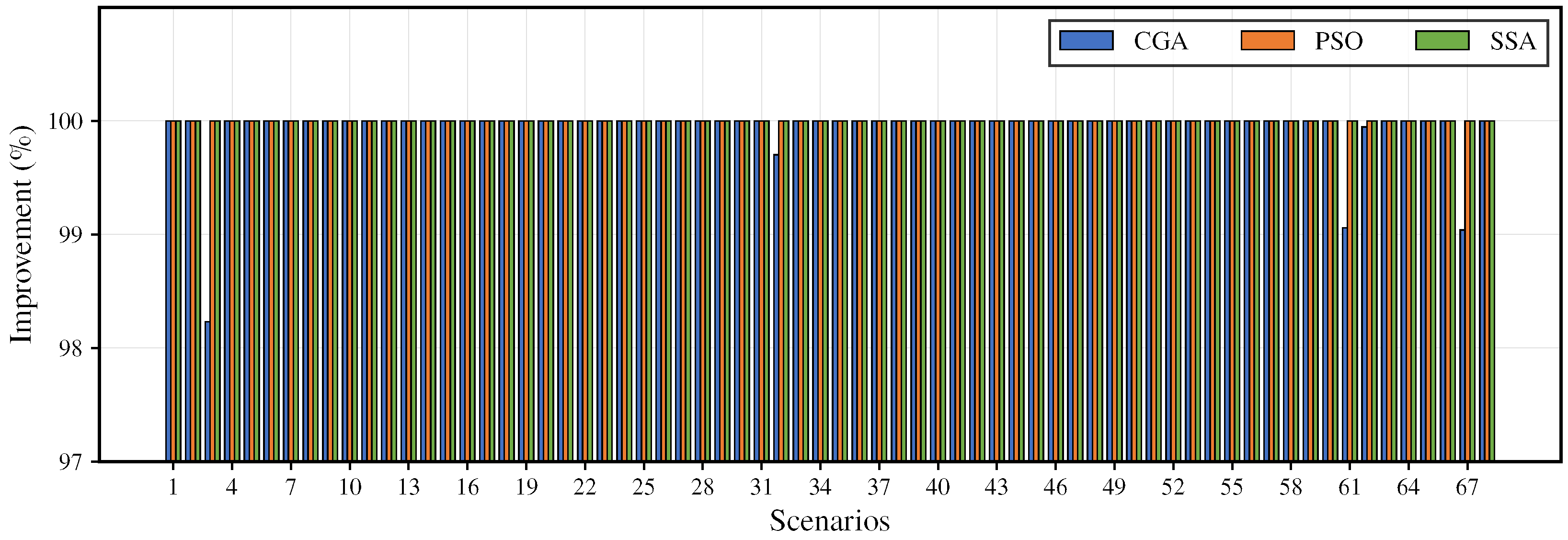
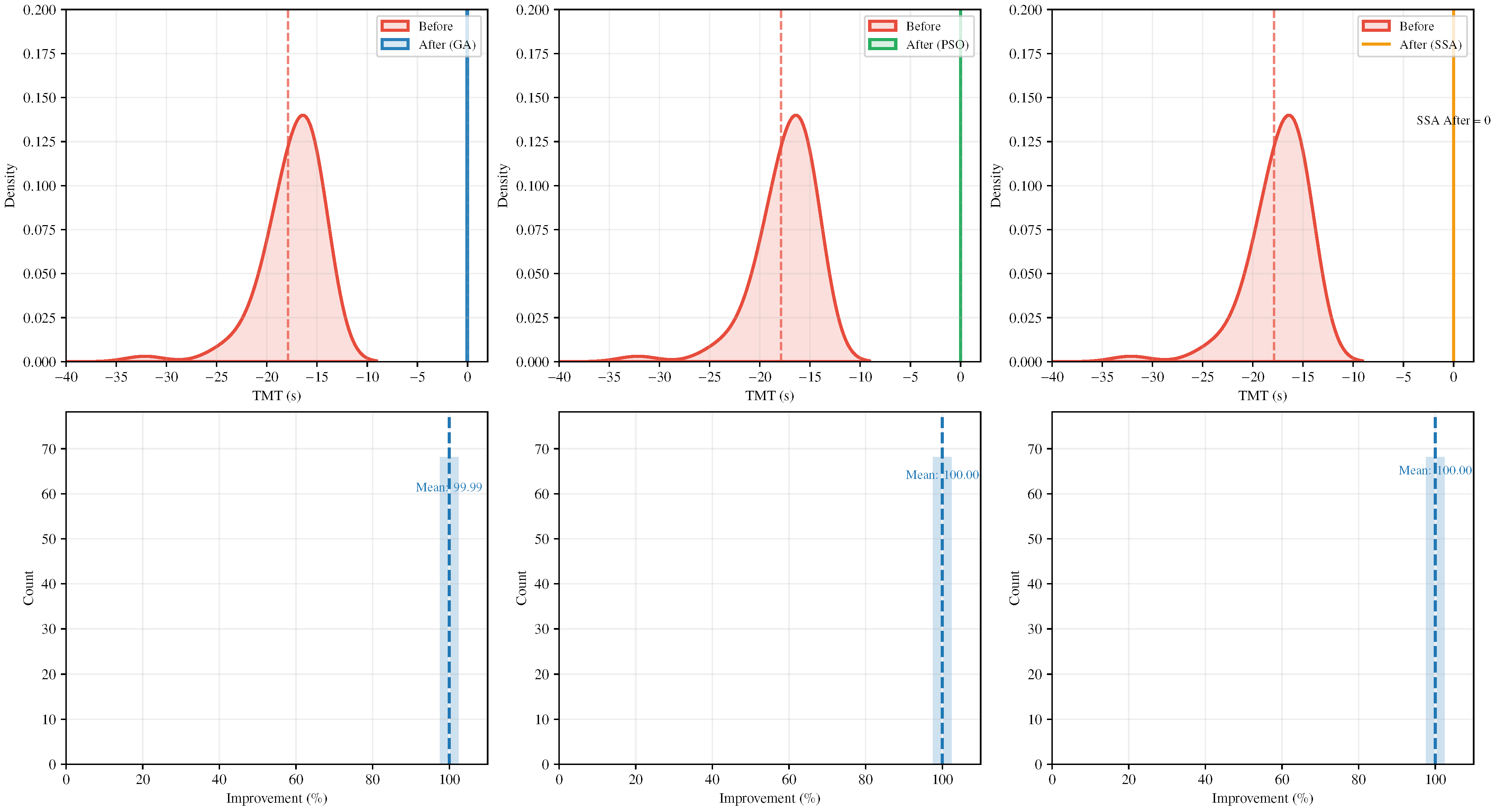
To strengthen the optimal implementation stage of the protection coordination by the CGA, PSO and SSA, Figure 10 and Figure 11 detail each of the important elements of this automation, where Figure 10 denotes the states of the coordinated scenarios and the optimal coordination percentage of the relay pairs, while Figure 11 shows the TMT before optimization and the TMT after the optimization process, and the TMT values where the different case studies remained coordinated by the CGA, PSO and SSA. Additionally, the information condensed in Figure 10 is reflected in

Table 8. TMT results per scenario for the evaluated algorithms.

Scenario	${\mathrm{GA}}_{\mathit{TMT}}$	${\mathrm{PSO}}_{\mathit{TMT}}$	${\mathrm{SSA}}_{\mathit{TMT}}$	Scenario	${\mathrm{GA}}_{\mathit{TMT}}$	${\mathrm{PSO}}_{\mathit{TMT}}$	${\mathrm{SSA}}_{\mathit{TMT}}$
1	0.000182	0.0	0.0	35	0.0	0.0	0.0
2	0.0	0.0	0.0	36	0.0	0.0	0.0
3	0.883930	0.0	0.0	37	0.0	0.0	0.0
4	0.0	0.0	0.0	38	0.0	0.0	0.0
5	0.0	0.0	0.0	39	0.0	0.0	0.0
6	0.0	0.0	0.0	40	0.0	0.0	0.0
7	0.0	0.0	0.0	41	0.0	0.0	0.0
8	0.0	0.0	0.0	42	0.0	0.0	0.0
9	0.0	0.000581	0.0	43	0.0	0.0	0.0
10	0.0	0.0	0.0	44	0.0	0.0	0.0
11	0.0	0.0	0.0	45	0.0	0.0	0.0
12	0.0	0.0	0.0	46	0.0	0.0	0.0
13	0.0	0.0	0.0	47	0.0	0.0	0.0
14	0.0	0.0	0.0	48	0.0	0.0	0.0
15	0.0	0.0	0.0	49	0.0	0.0	0.0
16	0.0	0.0	0.0	50	0.0	0.0	0.0
17	0.0	0.0	0.0	51	0.0	0.0	0.0
18	0.0	0.0	0.0	52	0.0	0.0	0.0
19	0.0	0.0	0.0	53	0.0	0.0	0.0
20	0.0	0.0	0.0	54	0.0	0.0	0.0
21	0.0	0.0	0.0	55	0.0	0.0	0.0
22	0.0	0.0	0.0	56	0.0	0.0	0.0
23	0.0	0.0	0.0	57	0.0	0.0	0.0
24	0.0	0.0	0.0	58	0.0	0.0	0.0
25	0.0	0.0	0.0	59	0.0	0.0	0.0
26	0.0	0.0	0.0	60	0.0	0.0	0.0
27	0.0	0.0	0.0	61	0.470611	0.0	0.0
28	0.0	0.0	0.0	62	0.026444	0.0	0.0
29	0.0	0.0	0.0	63	0.0	0.0	0.0
30	0.0	0.0	0.0	64	0.0	0.0	0.0
31	0.0	0.0	0.0	65	0.0	0.0	0.0
32	0.149056	0.0	0.0	66	0.0	0.0	0.0
33	0.0	0.0	0.0	67	0.479828	0.0	0.0
34	0.0	0.0	0.0	68	0.0	0.0	0.0

, which reports the TMT results for all analyzed scenarios and for each optimization algorithm applied. This was included to further support the validity of the outcomes obtained in the optimal coordination process of the relay pairs. Overall, the analysis shows that the optimization algorithms achieve a precision level of 99.99% in terms of relay pair optimal coordination with respect to the TMT metric.

The improvement percentages for each of the scenarios are detailed in Figure 11, which allows us to observe the total average improvement of all scenarios and, in turn, the minimum improvement value within all the optimal coordination validations carried out using the CGA; this indicates that the implementation of this type of methodologies guarantees coordination compared to the use of manual or heuristic methods.

The optimization of the CGA, PSO, and SSA allows, as shown in Figure 11, the analysis of the behavior of the scenarios before and after optimal coordination and ensures optimal management of the coordination of the different scenarios of the relay pairs.

In the edge computing environment, the algorithms exhibited execution times that differed between methods and depended on the scenario, as shown in

Table 9. Results obtained in Edge Computing for the execution times of the different optimization algorithms.

Scenario	CGA (s)	PSO (s)	SSA (s)	Scenario	CGA (s)	PSO (s)	SSA (s)
1	12.968	1.042	120.980	35	2.703	1.107	159.915
2	3.212	0.964	114.720	36	12.172	0.754	119.627
3	2.642	0.858	109.837	37	1.874	0.970	109.279
4	12.356	0.949	116.023	38	4.285	0.895	112.157
5	10.690	1.045	108.781	39	4.548	0.804	109.238
6	3.204	1.001	110.749	40	1.961	0.770	109.771
7	5.941	1.012	114.495	41	5.099	0.764	112.063
8	3.653	0.739	114.295	42	4.776	0.896	113.660
9	4.048	1.029	112.397	43	2.094	0.847	111.791
10	3.628	0.997	118.409	44	2.269	1.032	111.067
11	2.964	1.154	106.126	45	2.277	0.849	110.033
12	3.140	0.767	110.979	46	8.735	2.440	109.677
13	4.936	0.878	110.193	47	1.606	0.967	115.060
14	5.479	1.322	106.315	48	1.958	1.044	114.510
15	4.026	0.962	111.714	49	1.934	0.930	113.819
16	6.327	0.939	109.906	50	3.852	1.311	111.689
17	2.821	0.806	110.403	51	2.927	1.078	115.356
18	4.769	1.042	111.099	52	11.772	1.020	111.382
19	1.844	0.786	114.801	53	3.159	1.027	111.866
20	4.934	0.886	116.043	54	5.825	1.023	117.741
21	12.352	0.667	125.068	55	5.985	1.071	122.194
22	3.862	0.944	118.074	56	3.028	0.789	116.975
23	3.169	0.907	124.069	57	2.378	0.819	114.017
24	6.765	1.006	117.999	58	6.054	0.857	114.432
25	2.644	0.781	115.050	59	3.512	0.884	119.491
26	3.902	0.858	110.445	60	13.580	0.962	129.802
27	12.551	0.974	119.328	61	3.660	1.309	134.236
28	11.857	1.171	118.514	62	14.285	1.408	144.015
29	5.405	1.128	114.332	63	4.619	1.056	129.063
30	3.679	0.812	119.716	64	13.870	1.292	135.580
31	12.400	1.278	117.431	65	5.373	1.250	137.959
32	3.321	0.832	115.146	66	3.993	1.058	137.066
33	2.485	0.926	113.372	67	2.917	0.903	135.786
34	7.811	0.978	127.846	68	14.085	0.944	141.288

. In general, a clear separation by order of magnitude can be observed: PSO yields the lowest runtimes, approximately between 0.667 s and 2.440 s; CGA shows intermediate runtimes, with executions around 1.606 s–14.285 s; whereas SSA presents the highest runtimes, in the order of 109.238 s–159.915 s. This scenario-to-scenario variability arises because each case imposes different conditions on relay pair coordination, which changes the difficulty of the tuning task and, consequently, the required computational effort for the task. Moreover, the differences among techniques are linked to their own convergence dynamics; in particular, bio-inspired methods may require more iterations or function evaluations to stabilize the solution, depending on the topology and constraints active in each scenario. Nevertheless, despite the observed temporal dispersion, the results confirm that all techniques are feasible for obtaining optimal coordination solutions, with PSO and CGA being especially competitive in terms of computational time, and SSA remaining consistent, albeit with a higher runtime cost under edge computing execution.

3.4. Comparison of Inverse-Time Overcurrent Curves

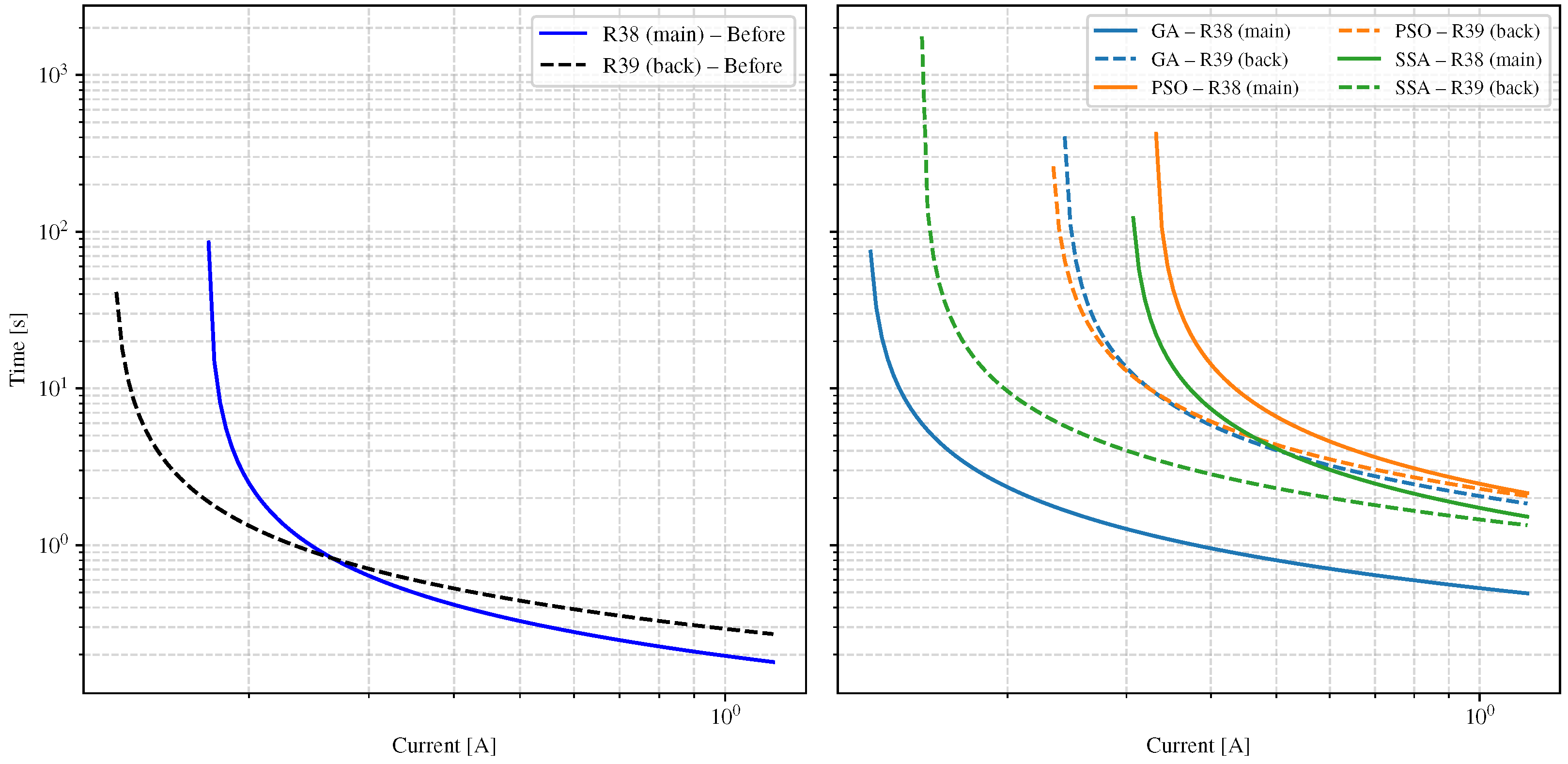
Figure 12 compares the time–current profiles of the relay pair R38–R39 before (left) and after (right) applying the optimization algorithms. Under the initial condition, the curves of both relays intersect, which indicates a lack of coordination for this relay pair when the automated process is initialized from the manual procedure. After optimization, the solutions obtained by each optimization algorithm are shown on the right-hand side and are identified by their corresponding colors.

In the figure, it can be observed that the intersections are eliminated, so that the profiles no longer cross and the required selectivity is satisfied, indicating sufficient coordination. In this sense, relay R38 clears significantly faster than R39, which is consistent with its role as the primary protection, whereas R39 operates as a backup while preserving the coordination margin provided by the optimization algorithms. The vertical axis represents the clearing time in seconds (s), whereas the horizontal axis corresponds to the fault current in amperes (A).

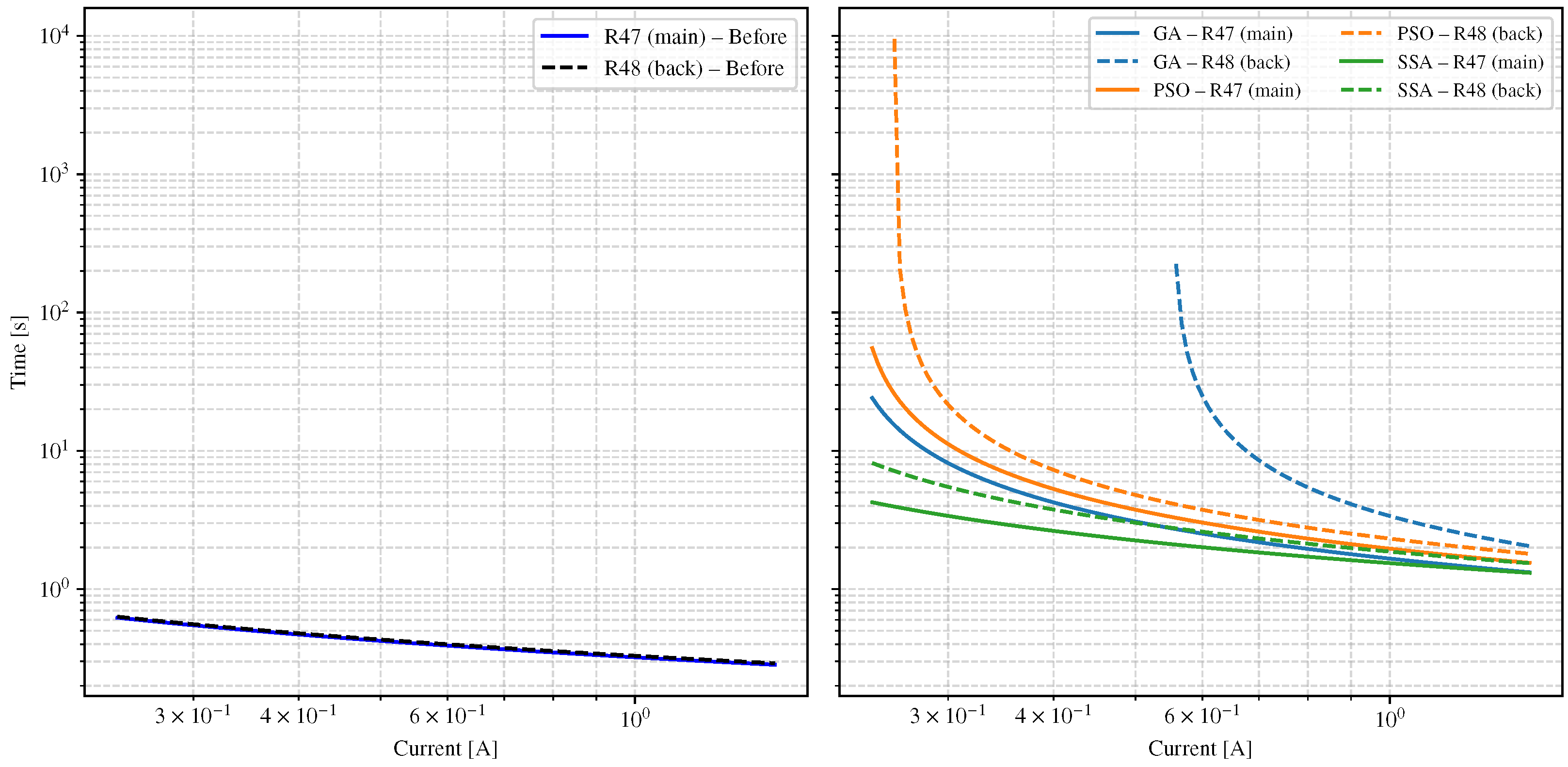
It is important to note that these results present only three examples among the many outcomes obtained from the different optimization algorithms applied to this relay pair coordination methodology. Figure 13 shows the second relay pair, R47–R48, before (left) and after (right) optimization. Under the initial condition, the two curves are excessively close when the automation is based on the manual procedure, resulting in a reduced coordination margin. In contrast, the right-hand side shows how the CGA, PSO, and SSA provide improved settings that yield a more suitable response, as the curves exhibit better coordination and reduced operating times for the same fault current. Overall, within the results obtained using this methodology, all optimization algorithms delivered satisfactory performance in coordinating the relay pairs.

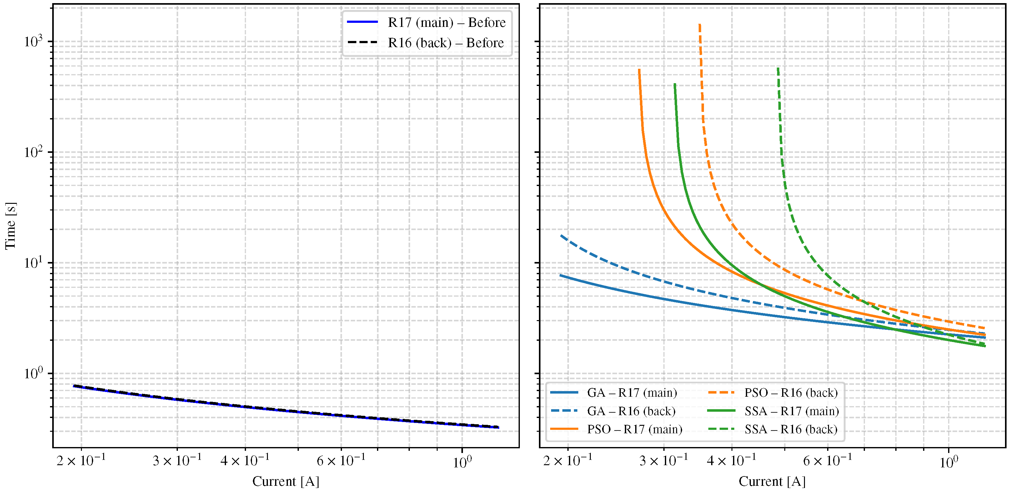
Finally, Figure 14 compares the time–current curves of the relay pair R17 (primary) and R16 (backup) before and after applying the optimization stage. In the “Before” case (right-hand side), both curves almost overlap, indicating a lack of selectivity and a high risk of simultaneous tripping between the primary protection and its backup. In contrast, the “After” case (left-hand side) shows the coordinated settings obtained using the CGA (blue), PSO (orange), and SSA (green). In all three cases, the primary relay R17 operated faster than R16 throughout the fault current range, and the curves did not intersect, confirming that the required coordination margin was met. Therefore, by comparing the behaviors of the different optimization algorithms and the applied methodology, it can be concluded that all the techniques satisfy the requirements for the optimal coordination of the relay pairs within the analyses presented in this study.

The algorithms were effective and reliable for solving complex protection coordination problems. This is useful because complex manual processes related to the coordination of various directional overcurrent protections can be replaced with simple automation and optimization methods. Because automation and optimization processes can be run for different operating conditions, this tool is useful for protection engineers and system operators who want to continually calculate settings, which is typically difficult with manual processes. In addition, these algorithms can be adjusted to achieve the desired outcome with other events that the operators consider.

4. Conclusions

This study presented an edge-computing-based architecture for the automatic and optimal coordination of directional inverse-time overcurrent relays in meshed MGs with DG. The proposed framework integrates a graph theory-based network model for topological awareness and fault path tracing, an automation stage that ensures feasible protection parameters under different operating conditions, and a comparative metaheuristic optimization stage that adjusts relay settings to reduce global miscoordination while preserving selectivity constraints for each candidate solution and each primary–backup relay pair.

From a methodological perspective, graph theory enables the representation of each operating condition as a connected directed graph and the automatic identification of fundamental meshes, fault locations, and primary–backup relay pairs. This automation is essential in meshed MGs, where bidirectional fault current contributions and frequent operational changes make manual pair identification slow and error-prone. Consequently, the proposed procedure constitutes a systematic and scalable mechanism to build the set of relay pairs required in coordination audits, considering multiple scenarios and fault points, and enabling a reproducible workflow for analysis and verification in environments with high operational variability.

The methodology was validated on a modified IEEE 33-bus system configured as a meshed MG, considering grid-connected and island modes, the charging and discharging states of two electric vehicle charging stations, and the presence and absence of photovoltaic generation. In total, 68 operating scenarios were evaluated by applying faults at 10% and 90% of the length of each protected line to enforce selectivity at both ends. Under these conditions, 100 primary–backup relay pairs were coordinated, demonstrating that the approach can handle complex and realistic coordination workloads and exceed the limited scope commonly reported in previous studies for microgrids with less demanding topologies.

In terms of performance, the automatic stage provided feasible protection settings, although residual miscoordination persisted under certain operating conditions. In contrast, the optimization stage implemented using CGA, SSA, and PSO substantially improved global coordination by driving the TMT index toward its desired value (close to zero), thus enhancing coordination quality relative to the automatic baseline. In the reported evaluation, SSA and PSO achieved the best coordination results, with performance close to complete coordination under the normalized TMT-based assessment, while CGA also yielded significant improvements, confirming the effectiveness of the edge-enabled optimization pipeline in strengthening selectivity and reducing global miscoordination in scenarios with high operational uncertainty.

The present validation was performed in a software-based environment in which the protection settings were computed and evaluated exclusively using numerical simulations. The practical implementation of the proposed protection scheme involves communication challenges that must be addressed in future studies. Each relay requires reliable communication channels to receive updated settings in response to changes in network operating conditions, which may require significant investment in communication infrastructure. The transmission of data over such communication systems also introduces cybersecurity concerns, including the risk of unauthorized access and malicious manipulation of protection settings. Furthermore, communication networks are inherently subject to latency, data corruption, and packet loss, all of which can adversely affect the dependability and operating speed of the protection systems. Communication failures can also lead to miscoordination between primary and backup protection relays, compromising system safety and overall reliability. Finally, the large-scale deployment of adaptive communication-based protection coordination schemes requires increased computational resources and communication bandwidth, which in turn results in more complex system architectures and higher implementation and maintenance costs.

In future work, experimental validation is proposed in a laboratory or real microgrid, including the direct deployment of settings to relays; integration of cybersecurity and secure communication layers (authentication, access control, and resilience against cyber events) consistent with edge-enabled schemes; latency- and reliability-aware coordination under partial connectivity between the cloud and edge nodes; and extension to more general relay models (multiple IEC/IEEE curves and dual-setting relays), as well as the explicit incorporation of uncertainty associated with renewable variability and measurement errors.

References

1. Asano, H.; Ishii, H.; Takano, H. Distributed energy resource integration for carbon neutral power systems: Market-based approaches to ancillary services and microgrid operation. IEEJ Trans. Electr. Electron. Eng. 2024, 19, 598–607. [Google Scholar] [CrossRef]
2. Kostenko, G.; Zaporozhets, A. Enhancing of the power system resilience through the application of micro power systems (microgrid) with renewable distributed generation. Sist. Res. Energ. 2023, 20233, 25–38. [Google Scholar] [CrossRef]
3. Altaf, M.W.; Arif, M.T.; Islam, S.N.; Haque, M.E. Microgrid protection challenges and mitigation approaches—A comprehensive review. IEEE Access 2022, 10, 38895–38922. [Google Scholar] [CrossRef]
4. Dagar, A.; Gupta, P.; Niranjan, V. Microgrid protection: A comprehensive review. Renew. Sustain. Energy Rev. 2021, 149, 111401. [Google Scholar] [CrossRef]
5. Serna-Montoya, L.F.; Saldarriaga-Zuluaga, S.D.; López-Lezama, J.M.; Muñoz-Galeano, N. Optimal Microgrid Protection Coordination for Directional Overcurrent Relays Through Mixed-Integer Linear Optimization. Energies 2025, 18, 2035. [Google Scholar] [CrossRef]
6. Shendi, A.J.; Mohammadian, L.; Ghanizadeh, R.; Pouladi, J.; Beiza, J. Optimal synchronization of overcurrent relays in active distribution networks using a hybrid genetic-differential optimization algorithm. Electr. Eng. 2025, 107, 7815–7830. [Google Scholar] [CrossRef]
7. Niranjan, P.; Choudhary, N.K.; Singh, N.; Singh, R.K. Optimal Coordination of Dual-Setting Directional Over Current Relay in Microgrid Considering Multi-Parametric Characteristics. J. Oper. Autom. Power Eng. 2025, 13, 174–183. [Google Scholar] [CrossRef]
8. Gairola, E.; Rawat, M.S.; Thakur, P.; Gupta, S.; Kumar, M. Comparative study of heuristic algorithms for coordination of industrial over current relays with nonstandard characteristics in microgrid protection. Sci. Rep. 2025, 15, 16020. [Google Scholar] [CrossRef] [PubMed]
9. Ayvaz, A. An improved walrus optimizer for optimal coordination of directional overcurrent relays in complex networks. J. Supercomput. 2025, 81, 1345. [Google Scholar] [CrossRef]
10. Wadood, A.; Albalawi, H.; Alatwi, A.M.; Park, H. Modified Swarm-Based Artificial Intelligence Optimization for Optimal Coordination of Directional Overcurrent Relays in Power System. IEEE Access 2025, 13, 71007–71026. [Google Scholar] [CrossRef]
11. Mohajer, F.; Kazemi Karegar, H.; Salemnia, A.; Sadeh, J. Optimal overcurrent relay coordination considering uncertainty of photovoltaic systems. Electr. Eng. 2025, 107, 9089–9107. [Google Scholar] [CrossRef]
12. Eladl, A.A.; Sheta, A.N.; Saeed, M.A.; Bureš, V.; Sedhom, B.E. Assessing the impact of distributed energy resources on overcurrent protection in microgrids for enhanced effectiveness. Results Eng. 2025, 25, 104461. [Google Scholar] [CrossRef]
13. Shad, H.; Amini Khanavandi, H.; Abrisham Foroushan Asl, S.; Aranizadeh, A.; Vahidi, B.; Mirmozaffari, M. Optimal Protection Coordination for Grid-Connected and Islanded Microgrids Assisted by the Crow Search Algorithm: Application of Dual-Setting Overcurrent Relays and Fault Current Limiters. Energies 2025, 18, 1601. [Google Scholar] [CrossRef]
14. Balasubramanian, S.; Preetha Roselyn, J.; Sundaravadivel, P. Enhancing Microgrid Protection through Adaptive Decentralized Relay Coordination: A Solution to Blinding and Symapthetic Tripping. IEEE Access 2025, 13, 138660–138675. [Google Scholar] [CrossRef]
15. Ghadiri, S.M.E.; Mazlumi, K. Adaptive protection scheme for microgrids based on SOM clustering technique. Appl. Soft Comput. 2020, 88, 106062. [Google Scholar] [CrossRef]
16. Brearley, B.; Prabu, R. A review on issues and approaches for microgrid protection. Renew. Sustain. Energy Rev. 2017, 67, 988–997. [Google Scholar] [CrossRef]
17. Ustun, T.S.; Ayyubi, S. Automated network topology extraction based on graph theory for distributed microgrid protection in dynamic power systems. Electronics 2019, 8, 655. [Google Scholar] [CrossRef]
18. Asl, S.A.F.; Gandomkar, M.; Nikoukar, J. Optimal protection coordination in the micro-grid including inverter-based distributed generations and energy storage system with considering grid-connected and islanded modes. Electr. Power Syst. Res. 2020, 184, 106317. [Google Scholar] [CrossRef]
19. Taylor, J.A.; Hover, F.S. Laplacians for flow networks. SIAM J. Discret. Math. 2011, 25, 1349–1364. [Google Scholar] [CrossRef]
20. IEC 60255-151; Measuring Relays and Protection Equipment—Part 151: Functional Requirements for Over/Under Current Protection. International Electrotechnical Commission: Geneva, Switzerland, 2009.
21. Korashy, A.; El-Dabah, M.; Amer, G. Modified water cycle algorithm for optimal overcurrent relay coordination. IET Gener. Transm. Distrib. 2019, 13, 1390–1398. [Google Scholar] [CrossRef]
22. Saldarriaga-Zuluaga, S.; Zuluaga, C.; Muñoz-Galeano, N.; López-Lezama, J. Optimal Coordination of Overcurrent Relays in Microgrids Using a Metaheuristic Approach. Int. J. Eng. Res. Technol. 2020, 13, 2213–2218. [Google Scholar] [CrossRef]
23. Zanjani, M.G.M.; Mazlumi, K.; Kamwa, I. Application of μPMUs for Adaptive Protection of Overcurrent Relays in Microgrids. IET Gener. Transm. Distrib. 2018, 12, 4061–4068. [Google Scholar] [CrossRef]
24. Piesciorovsky, E.; Schulz, N. Fuse Relay Adaptive Overcurrent Protection Scheme for Microgrid with Distributed Generators. IET Gener. Transm. Distrib. 2017, 11, 540–549. [Google Scholar] [CrossRef]
25. Memon, A.A.; Kauhaniemi, K. Protection of the future harbor area AC microgrids containing renewable energy sources and batteries. IEEE Access 2023, 11, 57448–57469. [Google Scholar] [CrossRef]
26. Sultana, U.; Rimsha, S.; Rashid, J. Genetic Algorithm-Based Optimal Protection Scheme for the Coordination of Bi-Directional Overcurrent Relays in a Carbon-Free AC Microgrid. Eng. Proc. 2023, 46, 27. [Google Scholar] [CrossRef]
27. Montano, J.; Guzman-Rodriguez, J.P.; Palomeque, J.M.; Gonzalez-Montoya, D. Comparison of different optimization techniques applied to optimal operation of energy storage systems in standalone and grid-connected direct current microgrids. J. Energy Storage 2024, 96, 112708. [Google Scholar] [CrossRef]
28. Grisales-Noreña, L.F.; Ocampo-Toro, J.A.; Montoya-Giraldo, O.D.; Montano, J.; Hernandéz, J. Optimal operation of battery storage systems in standalone and grid-connected DC microgrids using parallel metaheuristic optimization algorithms. J. Energy Storage 2023, 65, 107240. [Google Scholar] [CrossRef]
29. Montano, J.; Mejia, A.F.T.; Rosales Munoz, A.A.; Andrade, F.; Garzon Rivera, O.D.; Palomeque, J.M. Salp swarm optimization algorithm for estimating the parameters of photovoltaic panels based on the three-diode model. Electronics 2021, 10, 3123. [Google Scholar] [CrossRef]
30. Montano, J.J.; Noreña, L.F.G.; Tobon, A.F.; Montoya, D.G. Estimation of the parameters of the mathematical model of an equivalent diode of a photovoltaic panel using a continuous genetic algorithm. IEEE Lat. Am. Trans. 2022, 20, 616–623. [Google Scholar] [CrossRef]
31. Montano, J.; Candelo-Becerra, J.E.; Hoyos, F.E. A Pareto Multiobjective Optimization Power Dispatch for Rural and Urban AC Microgrids with Photovoltaic Panels and Battery Energy Storage Systems. Electricity 2025, 6, 68. [Google Scholar] [CrossRef]
32. Montano, J.; Guzmán, J.P.; Garzón, O.D.; Barrera, A.M.R. Techno-economic approach for energy management system: Multi-objective optimization algorithms for energy storage in standalone and grid-connected DC microgrids. J. Energy Storage 2024, 102, 114069. [Google Scholar] [CrossRef]
Figure 1. Architecture used to obtain the optimal overcurrent protection settings.
Electricity 07 00014 g001
Figure 2. General procedure for determining the directional overcurrent settings with automated and optimization processes.
Electricity 07 00014 g002
Figure 3. Modified scheme of the IEEE 33-bus system as a meshed MG with DG and EVCS.
Electricity 07 00014 g003
Figure 4. Automation algorithm for calculating protection settings.
Electricity 07 00014 g004
Figure 5. Optimal coordination of overcurrent protection relays.
Electricity 07 00014 g005
Figure 6. Adjacency matrix.
Electricity 07 00014 g006
Figure 7. Fundamental loops of the modified IEEE 33-bus system. Blue indicates each loop identified in the network with the algorithm.
Electricity 07 00014 g007
Figure 8. Protection relay influence network.
Electricity 07 00014 g008
Figure 9. TMT calculated by scenario.
Electricity 07 00014 g009
Figure 10. Percentage of optimal coordination of different relay pair scenarios.
Electricity 07 00014 g010
Figure 11. Comparison of TMT with the automated and optimal protection settings. Dashed red line refers to the mean of the TMT for the base case and dashed blue line corresponds to the mean of improvement percentage.
Electricity 07 00014 g011
Figure 12. Comparison of the protection settings calculated for the relays R38 (blue) and R39 (black) with the (left) automatic process and (right) optimization algorithms process.
Electricity 07 00014 g012
Figure 13. Comparison of the protection settings calculated for the relays R47 (blue) and R48 (black) with the (left) automatic process and (right) optimization process.
Electricity 07 00014 g013
Figure 14. Comparison of the protection settings calculated for the relays R17 (blue) and R16 (black) with the (left) automatic process and (right) optimization process.
Electricity 07 00014 g014