Article

Experimental Study of Methanol Leak and Diffusion in Open-Channel Flow

1
PipeChina Institute of Science and Technology, Tianjin 300450, China
2
College of Mechanical and Transportation Engineering, China University of Petroleum (Beijing), Beijing 102249, China
*
Author to whom correspondence should be addressed.
Pollutants 2026, 6(3), 40; https://doi.org/10.3390/pollutants6030040
Submission received: 15 April 2026 / Revised: 27 July 2026 / Accepted: 28 July 2026 / Published: 4 August 2026
(This article belongs to the Section Water Pollution)

Abstract

Methanol is highly soluble and with spreads quickly in natural water bodies, which could bring about serious environmental risks if leaked. In the present work, the transport and diffusion behavior of methanol in an open-channel flume under controlled hydraulic conditions is investigated experimentally. A closed-loop experimental system was designed to mimic the pipeline leakage scenarios and image-based reconstruction methods were applied to quantify the spatiotemporal evolution of the methanol concentration fields. Systematic analysis was performed on the effects of flow velocity, water depth, leakage rate and leakage location. The results indicate that flow velocity is the dominant factor controlling the downstream advective transport, with increasing velocity significantly reducing the downstream extent of high-concentration zones. Water depth affects vertical mixing and dilution capacity, with deeper flows maintaining more persistent plume structures. Higher leak rates result in higher local concentrations and larger near-field contaminated regions. The position of the leakage is also very important for the plume morphology: the boundary effects lead to a limited and asymmetric dispersion when the leakage is close to the boundary, while the dispersion is more symmetric when the leakage is in the middle of the domain. The study highlights the combined roles of advection, turbulent mixing and boundary confinement in governing methanol plume evolution. The results provide experimental evidence for the understanding of soluble pollutant transport mechanisms in open-channel flows under simplified hydraulic conditions.

1. Introduction

The accidental release of hazardous chemicals into aquatic environments represents an important environmental challenge associated with industrial production, storage, and transportation activities [1]. With the continuous expansion of chemical transportation networks, pipeline leakage incidents involving liquid organic chemicals have become an increasing concern due to their potential impacts on aquatic ecosystems, water resources, and human activities. Once released into rivers or other flowing water bodies, dissolved pollutants are transported through complex physical processes, including advection, turbulent mixing, molecular diffusion, and dispersion, resulting in the formation of transient contamination plumes with highly variable spatial and temporal distributions [2,3,4]. Accurate prediction of pollutant migration characteristics is therefore essential for environmental risk assessment, emergency response, and the development of effective mitigation strategies.
Methanol is one of the most widely produced and transported organic chemicals and is extensively applied in chemical manufacturing, fuel production, and energy-related industries. Because of its complete miscibility with water and high mobility in aquatic environments, methanol released from pipelines or storage facilities can rapidly dissolve and spread within surrounding water bodies. Although methanol can be naturally degraded under suitable environmental conditions, elevated concentrations may cause adverse effects on aquatic organisms. Previous toxicological studies have demonstrated that methanol exposure can produce acute biological effects on fish, crustaceans, and other aquatic species, particularly when dilution and degradation processes are insufficient [5,6]. In addition, environmental fate investigations have indicated that the physicochemical properties of organic chemicals, including solubility, transportability, and persistence, strongly influence their migration behavior after entering aquatic systems [7,8]. Therefore, understanding the transport and dilution characteristics of methanol following accidental leakage is important for evaluating ecological risks and developing emergency response approaches.
The transport behavior of soluble pollutants in open-channel environments is controlled by the interaction between mean flow advection, turbulent diffusion, and hydrodynamic boundary conditions. Recent investigations have demonstrated that longitudinal and transverse dispersion in open channels are governed by the combined effects of velocity gradients, turbulence structures, and channel-scale hydraulic characteristics [9,10]. Subsequent investigations have demonstrated that channel geometry, flow velocity, water depth, and turbulence structures significantly influence pollutant spreading and concentration attenuation in natural and artificial channels [11,12,13,14]. Numerical transport models based on advection–dispersion equations and transient storage concepts have further improved the prediction of contaminant migration in river systems [15,16]. However, most existing studies have focused on general dissolved pollutants or conservative tracers, while the specific transport characteristics of highly soluble organic liquids released from localized leakage sources remain insufficiently understood.
Compared with conventional dissolved pollutants, methanol leakage exhibits several distinct transport characteristics. Due to its low molecular weight, high solubility, and negligible settling behavior, methanol rapidly interacts with surrounding water after release. The initial leakage stage involves strong coupling between the momentum of the released jet and ambient flow turbulence, which determines the subsequent development of the contamination plume. Previous studies on turbulent jets and environmental discharge processes have demonstrated that near-field mixing characteristics strongly regulate plume development, downstream concentration evolution, and dilution efficiency [17,18,19]. In open-channel environments, lateral boundaries and channel geometry further modify plume development by restricting transverse spreading and altering local turbulence structures [20,21,22]. Nevertheless, the combined effects of leakage location, source intensity, and hydraulic conditions on methanol plume evolution have not been systematically quantified.
In practical scenarios, pipeline leakage may occur at different locations, including submerged riverbeds, channel centers, and near-bank regions. These different leakage configurations can generate distinct transport behaviors. For example, bottom leakage may produce submerged jets with enhanced vertical mixing, whereas surface leakage may promote horizontal spreading along the water surface. In addition, bank confinement can reduce lateral dilution and increase pollutant residence time, resulting in asymmetric concentration distributions. Although computational fluid dynamics (CFD) approaches have been increasingly applied to simulate pollutant dispersion and investigate the influence of turbulence characteristics, diffusion coefficients, and boundary conditions [23,24,25,26], experimental investigations remain essential for validating transport mechanisms because transient leakage processes involve complex interactions between source momentum, turbulent mixing, and three-dimensional plume evolution.
Accurate characterization of pollutant concentration fields is also a major challenge in experimental studies. Conventional sampling methods provide concentration information only at discrete locations and may fail to capture the rapid spatial evolution of transient pollution plumes. Optical visualization techniques, including planar laser-induced fluorescence (PLIF) and image-based concentration reconstruction methods, have therefore been widely applied in fluid mixing studies because they provide non-invasive measurements with high spatial resolution [27,28,29]. Previous studies have demonstrated that optical measurement techniques, particularly laser-induced fluorescence methods, can effectively characterize scalar transport processes, quantify mixing efficiency, and resolve spatial concentration distributions in aqueous flows [30,31]. Furthermore, investigations of turbulent jets and plumes have demonstrated that entrainment processes and turbulent structures play critical roles in governing scalar transport, dilution, and dispersion of released fluids [32,33,34].
To address these knowledge gaps, this study experimentally investigates the leakage and diffusion behavior of methanol in an open-channel flow environment. A recirculating open-channel experimental system was developed to simulate localized pipeline leakage, and an image-based concentration reconstruction method was established to quantify the spatial evolution of methanol concentration fields. The effects of flow velocity, water depth, leakage rate, and leakage location on plume development were systematically examined. The objectives of this study are to (i) characterize the transport behavior of methanol under different hydraulic and leakage conditions, (ii) quantify the evolution of high-concentration contamination zones, and (iii) clarify the coupled roles of advection, turbulent mixing, and boundary confinement in controlling methanol dispersion. The results provide experimental insights into soluble pollutant transport mechanisms and support improved environmental risk assessment and emergency response strategies for chemical leakage accidents.

2. Experimental Methods

2.1. Experimental System

The experimental setup is a circular water tank, as shown in Figure 1a, with an overall length of 2.9 m, an overall width of 0.94 m, a channel width of 0.3 m, and a wall thickness of 1 cm. To facilitate clear observation and photographic recording of methanol diffusion after a leak, the channel was made from a transparent material, Plexiglas (Evonik Degussa, Shanghai, China). As shown in Figure 1b, the experimental system includes: (1) the circular tank, serving as the river channel; (2) a brushless motor blade array providing the driving force of water flow; (3) upstream flow-guiding channels positioned before the blades to reduce energy losses; (4) a camera monitoring system for recording the methanol diffusion; (5) an aluminum profile support frame; (6) a delivery pump system for controlling methanol leak mass flow rate; and (7) a PWM signal output system for regulating motor rotational speeds.

2.2. Experimental Procedure

The experiments were conducted in a recirculating open-channel flume system designed to investigate methanol dispersion under controlled hydraulic conditions. The overall procedure followed a sequential workflow including flow stabilization, leakage initialization, tracer injection, synchronized imaging, and post-processing.
  • Flow establishment and hydraulic control
At the beginning of each experiment, the flume was filled to the target water depth and allowed to stabilize for at least 10 min to ensure fully developed flow conditions. The flow field was generated using a brushless motor-driven circulation system controlled by an STM32F409-based module (STMicroelectronics, Shanghai, China), which allowed precise regulation of rotational speed and therefore hydraulic conditions.
Streamwise velocity was measured using a portable electromagnetic velocity meter (LS300-A portable electromagnetic velocity meter (Weifang Jinshui Huayu Information Technology Co., Ltd., Weifang, China)) at the leakage location. The measurement point was fixed at 60% of the local water depth, which provides a reliable approximation of depth-averaged velocity in turbulent open-channel flows. Each velocity value was obtained by time averaging over 60 s (1 Hz sampling), resulting in a coefficient of variation within ±5%, indicating stable and repeatable flow conditions across all tests.
2.
Leakage position and tracer injection
The leak opening was placed either at the channel bed or at the water surface, depending on the experimental configuration. The opening was simulated using a stainless-steel tube (inner diameter 2.0 mm, outer diameter 5.0 mm) with a controlled orifice representing a localized pipeline failure.
Prior to each experiment, methanol and a water-soluble acidic dye (Hangzhou Tianya Industrial Co., Ltd., Hangzhou, China) were pre-mixed in a fixed proportion to form a homogeneous dyed methanol solution. This pre-mixed solution was then injected into the flume through the leak tube using a high-precision syringe pump (Longer Precision Pump Co., Ltd., Baoding, China), ensuring accurate control of the mass flow rate. The dye concentration in methanol was kept constant across all tests to maintain a consistent optical calibration.
3.
Imaging system and environmental control
The evolution of the methanol plume was recorded using a synchronized dual-camera system (Hikrobot, Hangzhou, China) operating at 25 frames per second. The overhead and side-view cameras were hardware-triggered, achieving a temporal synchronization accuracy of ±5 ms.
Spatial resolutions of the reconstructed concentration fields were 0.8 mm/pixel (top view) and 0.6 mm/pixel (side view), respectively.
All experiments were conducted in a fully darkened laboratory environment. A constant-intensity LED panel (Guangdong Photon Lighting Co., Ltd., Zhongshan, China) provided uniform illumination. Background images were acquired before each test and subtracted from experimental images to eliminate fixed-pattern noise and illumination non-uniformity. Camera settings (exposure, gain, and ISO) were kept constant throughout all experiments.
The temperature was maintained at 22 ± 1 °C to ensure stable fluid properties.
4.
Experimental duration, repeatability, and data processing
Each experimental run lasted 5 s after the start of methanol injection, corresponding to the early transient stage of plume evolution. All results therefore represent transient dispersion behavior rather than steady-state conditions.
Each case was repeated three times under identical hydraulic and injection conditions. The variation between repeated runs remained within 6–8%, demonstrating high experimental repeatability. Ensemble-averaged fields were used for analysis unless otherwise stated.
Image processing included lens distortion correction, cropping, greyscale conversion, and background subtraction. No temporal averaging was applied in order to preserve the instantaneous structure of the plume. The concentration field at t = 5 s was selected as the representative state for comparative analysis.
Although turbulence intensity and full velocity profiles were not measured due to instrumentation limitations, the flow was carefully controlled to ensure fully developed turbulent conditions, and the measured point velocity reliably represents bulk flow behavior for comparative analysis.

2.3. Experimental Conditions

To characterize the flow regime and assess the scale of the experiments, key dimensionless numbers were calculated. The calculated ranges of the Reynolds number and Froude number for all experimental conditions are summarized in Table 1.
R e = u H ν
where Re is the flow Reynolds number, u is the cross-sectional average flow velocity (m/s), H is water depth (m), and ν is the kinematic viscosity of water (m2/s).
F r = u g H
where Fr is the Froude number, u is the cross-sectional average flow velocity (m/s), g is the gravitational acceleration (9.8 m/s2), and H is the water depth (m).
The Reynolds number ranged from approximately 2.2 × 10⁴ to 2.7 × 10⁵ across all test conditions, indicating that the flow was fully turbulent in all cases. The Froude number ranged from 0.06 to 0.34, which is characteristic of subcritical open-channel flow, consistent with typical lowland river conditions.
The experimental conditions employed in this study are summarized in Table 2.
The ranges of flow velocity and leak rate employed in the experiments were primarily constrained by the dimensions of the recirculating flume and the output range of the syringe pump. The flow velocities represent the range over which the current driving system can maintain stable operation and provide accurate measurements. The leak rates are determined by the pump’s flow rate range and the inner diameter of the leak tube (2.0 mm). The water depths (0.135–0.40 m) are limited by the side wall height of the flume and the position of the optical observation windows. These parameters thus reflect the feasible range under the physical constraints of the present experimental system.
The methanol exit velocity vj at the nozzle outlet was calculated from the volumetric flow rate Q set by the syringe pump, using the following relation:
v j = 4 Q π d 2
where d = 2.0 mm is the inner diameter of the leak tube. Based on this relation, the investigated flow rates (20–86.18 mL/min) correspond to exit velocities ranging from 0.106 to 0.457 m/s. In the following discussion, the term “leak velocity” refers specifically to this calculated exit velocity.

2.4. Image Processing

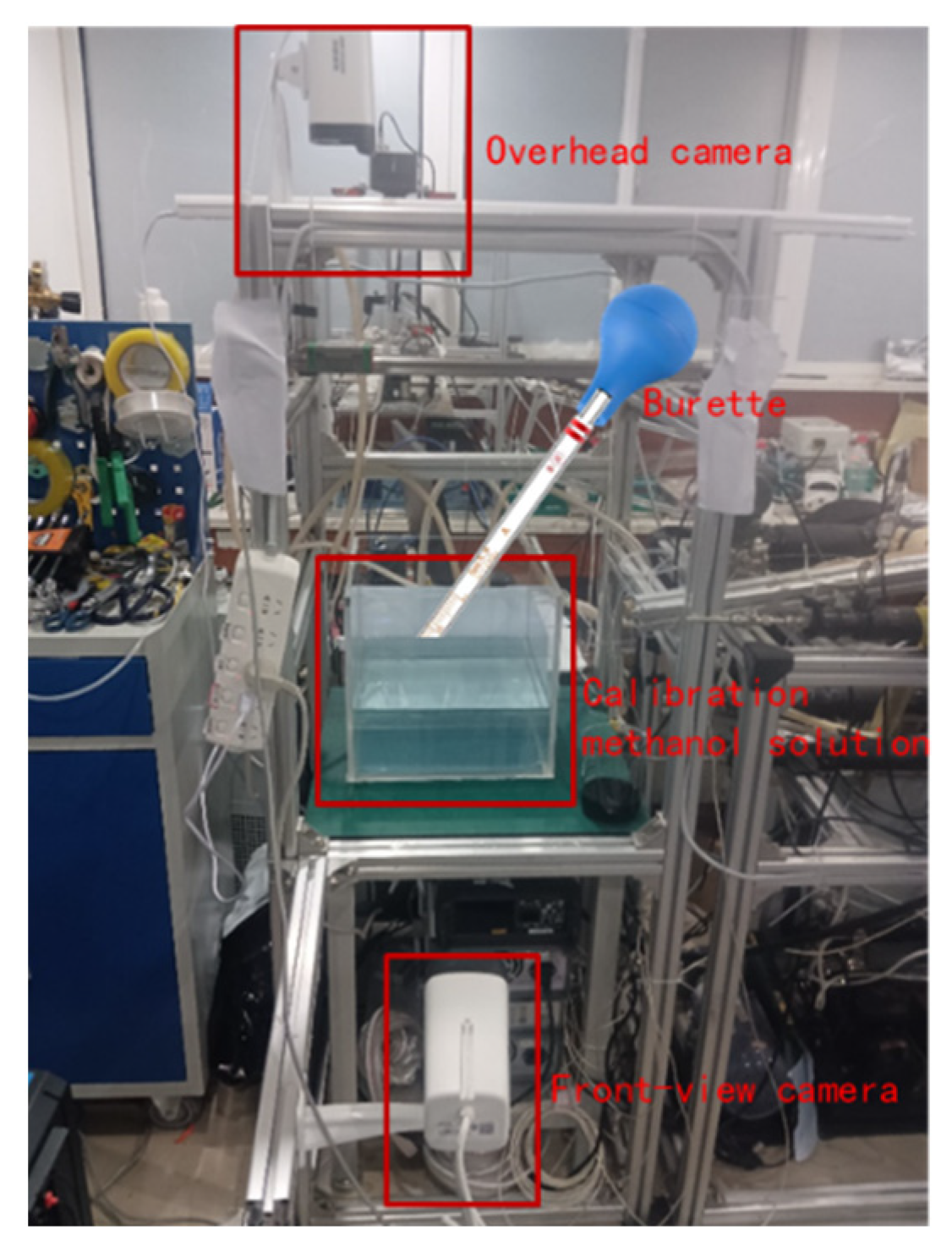
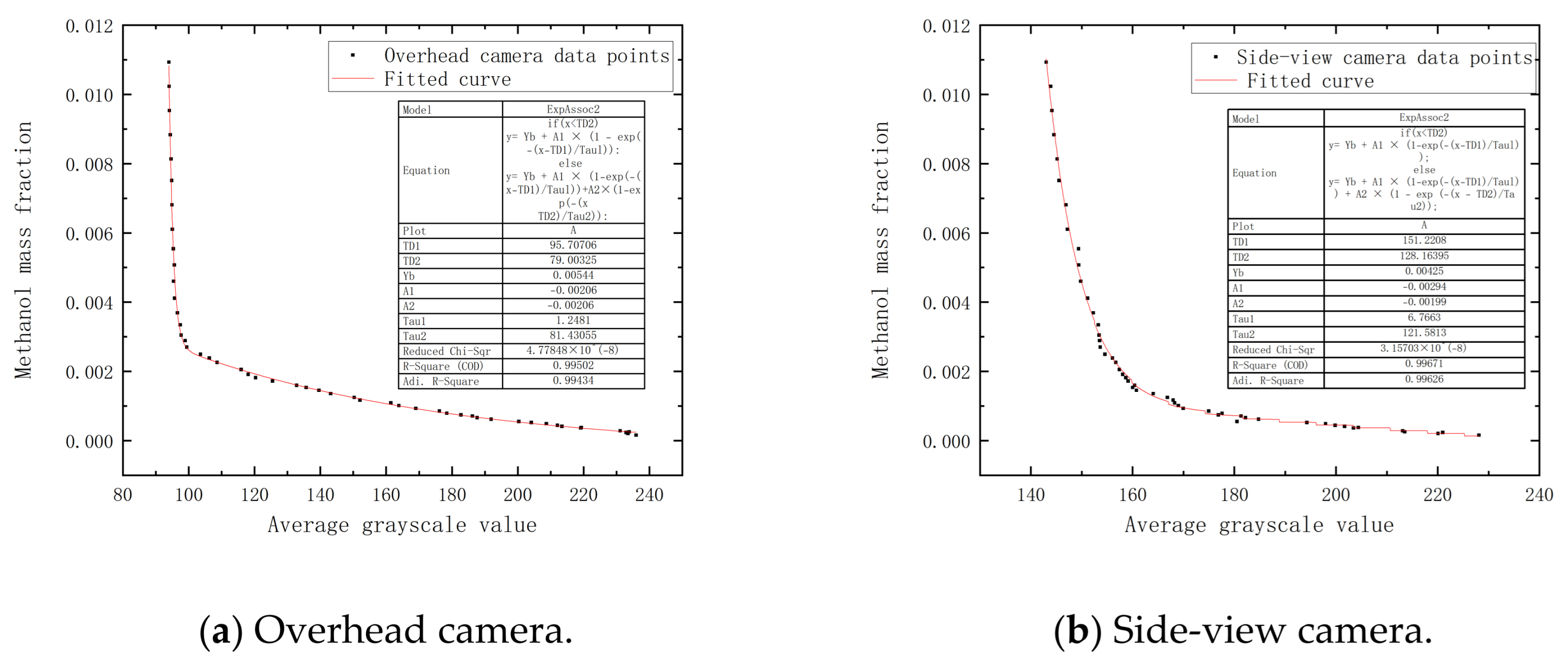
To transfer grey images of diffusion-dyed methanol into concentration contours, calibration experiments were conducted to obtain the relationship between the methanol concentration and the corresponding image greyscale values. As shown in Figure 2, a tank made from the same material as the circular tank was manufactured for the calibration. Both overhead and side-view cameras at the same shooting distances as in the diffusion tests were installed. Methanol with dye concentration was added into the water in the calibration tank. Greyscale values were obtained by analyzing the images. The corresponding methanol concentration was recorded by calculating the methanol quality added into the water in the tank. Varying the methanol concentration and recording the image greyscale value, empirical correlations between methanol concentration and image greyscale value could be obtained for overhead and side-view cameras.
Standard methanol solutions with dye concentrations identical to those used in the leak experiments were prepared at over 10 concentration levels ranging from 0 to 1500 mg/L, which covers the lethal threshold of 800 mg/L.
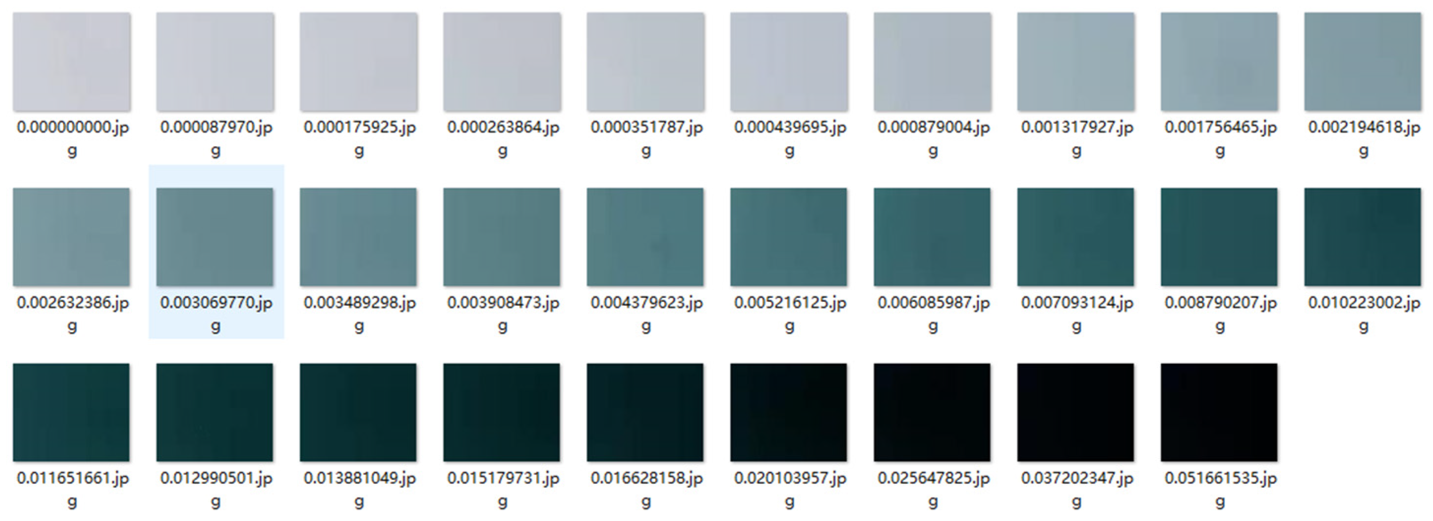
Images for several methanol concentration solutions are shown in Figure 3. The image turns darker with increasing methanol concentration. The correlation curve, relating average methanol concentration to image greyscale value, is shown in Figure 4.
Preliminary evaluations of simpler calibration models, including linear regression and single-term exponential functions, revealed systematic deviations in both the low-concentration range near the lethal threshold of 800 mg/L and the high-concentration range. These deviations were attributed to the nonlinear characteristics of the greyscale–concentration relationship, possibly associated with light scattering and dye distribution effects. To represent this nonlinear response over the entire concentration range while maintaining a smooth transition between concentration regimes, a piecewise exponential function was adopted as an empirical calibration relationship. The calibration dataset comprised more than 30 measurement points distributed across over 10 concentration levels ranging from 0 to 1500 mg/L. The piecewise exponential model includes seven fitted parameters, providing a sufficient number of calibration observations relative to the model complexity. The reduced chi-square value of 3.16 × 10⁻⁸ and the coefficient of determination (R2 = 0.9967) indicate strong agreement between the model predictions and calibration measurements. Nevertheless, these goodness-of-fit metrics alone cannot definitively exclude overfitting. In the present study, the risk of overfitting was reduced by limiting model complexity and maintaining an adequate calibration point-to-parameter ratio. Although independent validation using an external dataset would further improve confidence in the model transferability, such validation was beyond the scope of the present calibration experiment.
The empirical correlation coefficients for the overhead and side-view images, derived from Figure 4, are listed in Table 3, with equations like the following.
For each concentration, images were captured in triplicate. The relationship between the average greyscale value and the methanol mass fraction was fitted using an empirical piecewise exponential function:
y = Y b + A 1 × 1 e x T D 1 τ 1 x < T D 2 Y b + A 1 × 1 e x T D 1 τ 1 + A 2 × 1 e x T D 2 τ 2 x T D 2
In Equation (1), x represents the greyscale value (0–255) of a pixel, and y is the corresponding methanol mass fraction (dimensionless). The parameters TD1 and TD2 are greyscale thresholds that define two concentration regimes (low and high); Yb is the background greyscale baseline; A1 and A2 are amplitude coefficients; τ1 and τ2 are decay constants. This piecewise exponential function was chosen to capture the non-linear relationship between dye concentration and image intensity, which saturates at high concentrations.
This empirical function was chosen to capture the slight nonlinearity observed in the dye–methanol–water system, which arises from light scattering and dye aggregation effects. The model yielded an excellent fit with R2 = 0.9967 and reduced chi-square = 3.16 × 10⁻⁸, confirming its reliability for greyscale-to-concentration conversion. The fitted coefficients for the overhead and side-view cameras are listed in Table 1. The overhead and side-view cameras were calibrated and analysed independently, as they capture the plume from different optical paths.
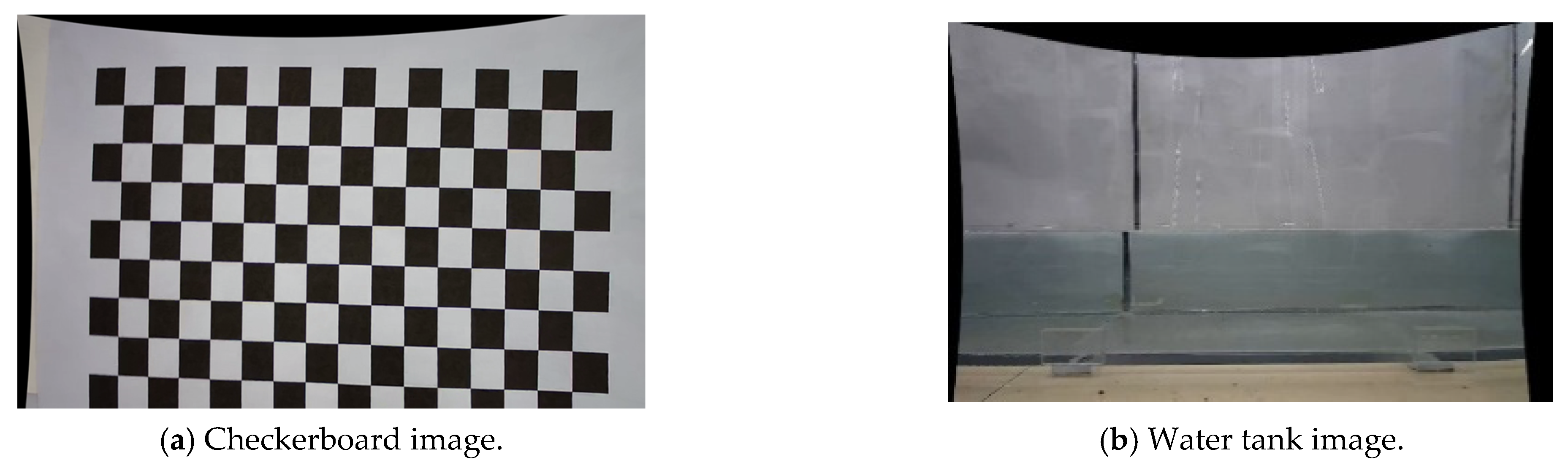
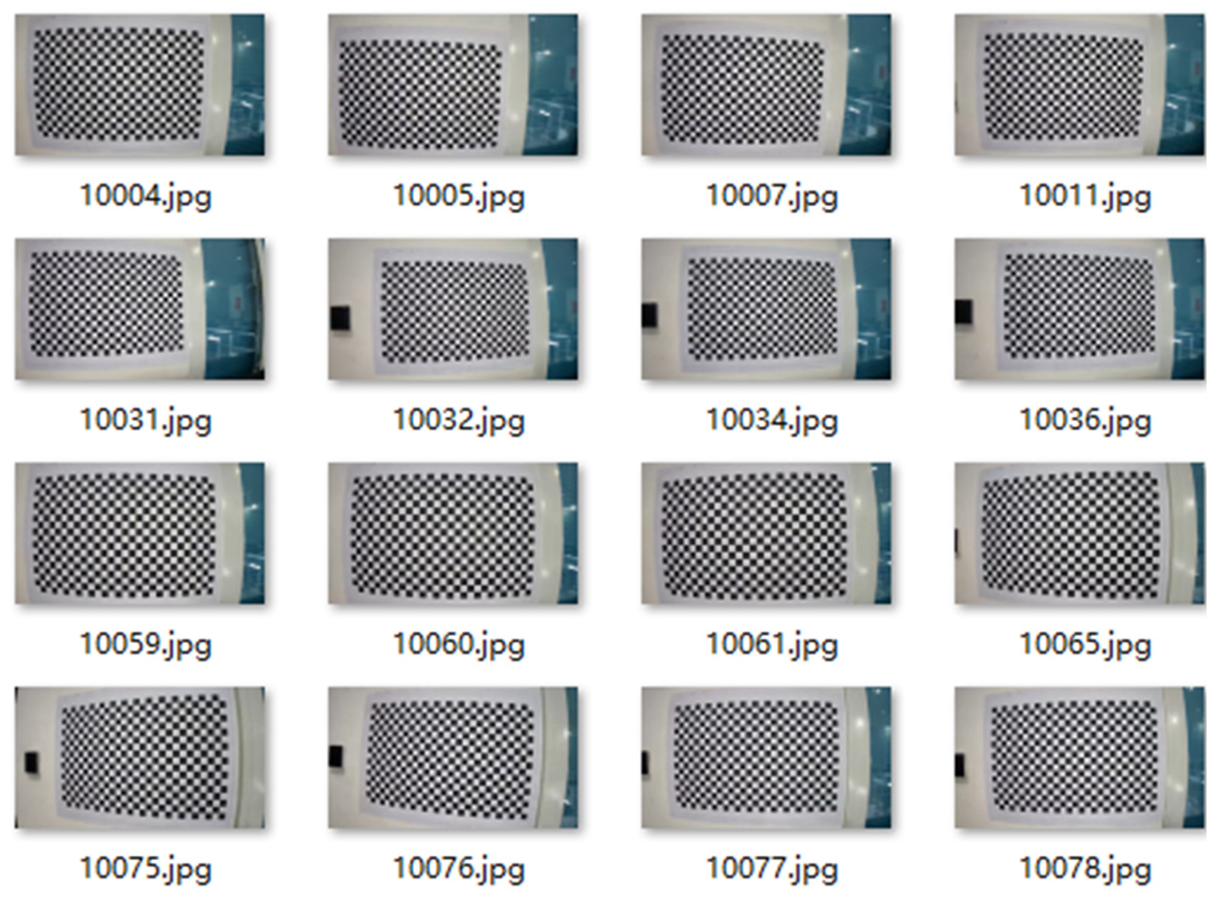
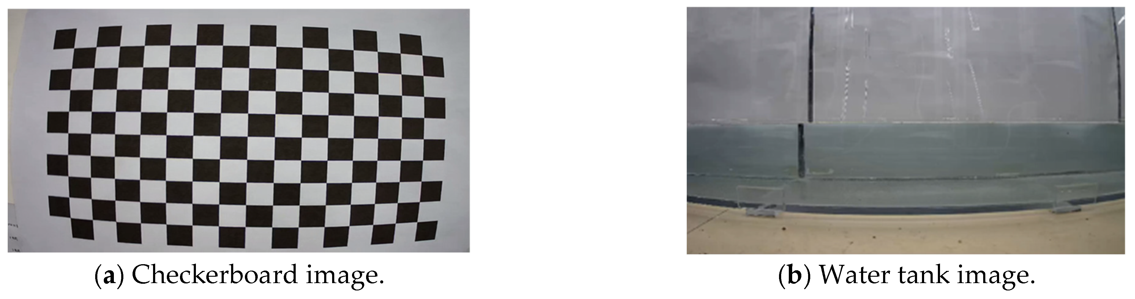
The cameras used in the experiments have self-zooming lenses, which cause image distortion. This problem can be solved using chessboard images captured at the same distance as the methanol diffusion processes, as shown in Figure 5. Image distortion correction algorithms were used to establish the matrix correspondences among the camera coordinate system, the pixel coordinate system, and the real-world coordinate system. This procedure allows the transformation of distorted images into geometrically corrected locations [35,36].
A chequerboard calibration pattern consisting of 27 × 17 interior corner points, with 1.9 cm spacing between adjacent corners, was used for camera calibration. Distorted images captured by the cameras (Figure 6) were analysed to determine the intrinsic parameters of each camera. Based on distortion correction theory, the images were then processed to remove distortion, resulting in the corrected images shown in Figure 7.
In the distortion correction, the matrix correspondences among the camera coordinate system, the pixel coordinate system, and the real-world coordinate system are defined.
S u v 1 = α γ u 0 0 β v 0 0 0 1 r 1 r 2 r 3 t X Y Z 1
where the terms on the right-hand side represent, from left to right, the camera coordinates, the pixel coordinates, and the real-world coordinates, respectively. Since the real-world coordinates are defined on the checkerboard plane, the Z-coordinate is 0.
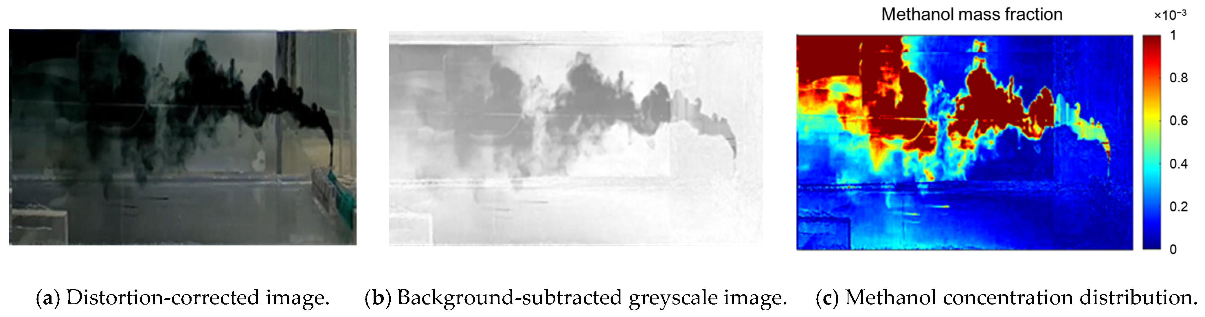
After obtaining the distortion-corrected experimental images (Figure 8a) via matrix transformation, a methanol diffusion image was first converted to a grey image. The greyscale values of this image were then subtracted from those of the background image without methanol diffusion, yielding the background-subtracted greyscale image shown in Figure 8b. Finally, by using the calibration correlation, the methanol mass concentration distribution contour was obtained from the greyscale image, as shown in Figure 8c.

2.5. Uncertainty Analysis

An uncertainty analysis was performed to quantify the reliability of the experimental measurements and the greyscale-based concentration reconstruction method. Each experimental condition was repeated three times to evaluate repeatability. The associated uncertainties include flow velocity measurement (±5%), leakage rate control (±2%), and greyscale-to-concentration conversion (±10%), the latter primarily arising from image acquisition stability and calibration fitting.
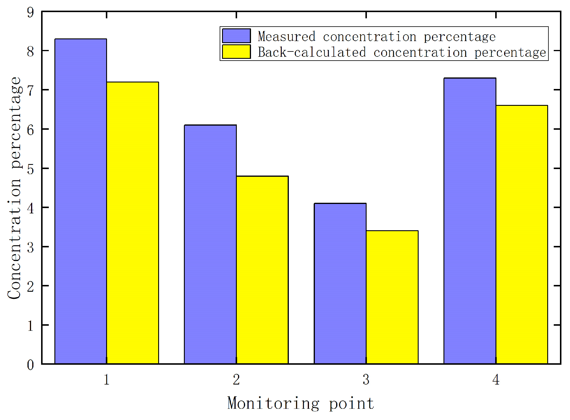
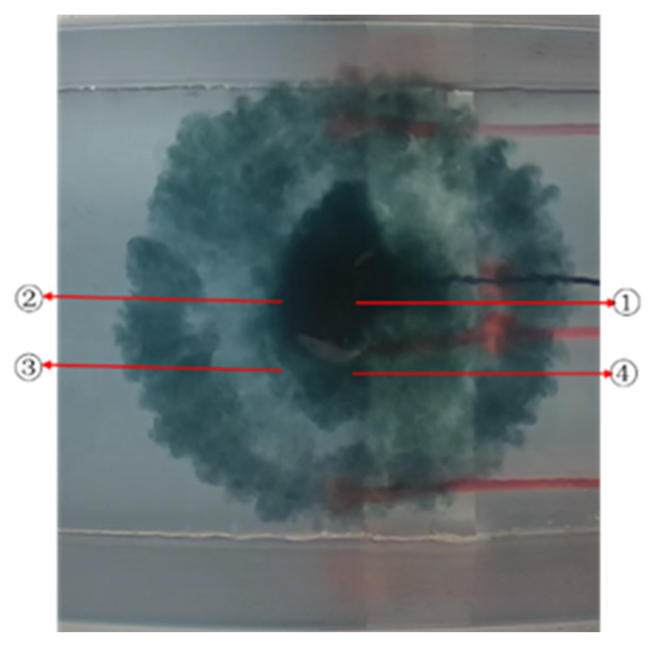
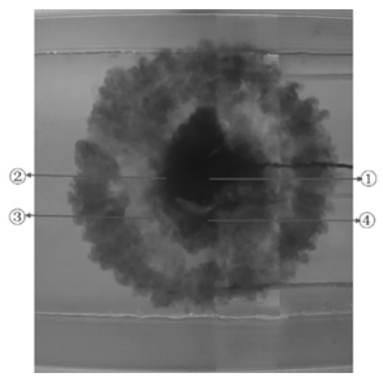
Standard uncertainty propagation was applied to combine these contributions, yielding an overall uncertainty of approximately ±13% for the reconstructed concentration field. As shown in Figure 9, the measured sampling concentrations and the back-calculated values at four monitoring locations exhibit strong quantitative agreement, with deviations consistently distributed within the calculated uncertainty range. In addition, the plume morphology presented in Figure 10 and its corresponding greyscale representation in Figure 11 show high spatial consistency, confirming the robustness of the image-based reconstruction framework for resolving methanol concentration distributions under the present experimental conditions.

3. Experimental Results and Discussion

Methanol concentrations in water exceeding 800 mg/L can be lethal to aquatic organisms, corresponding to a methanol mass fraction of approximately 8 × 10⁻⁴. In this study, this value is used to define the lethal threshold for methanol pollution [6].

3.1. Effect of Water Flow Velocity

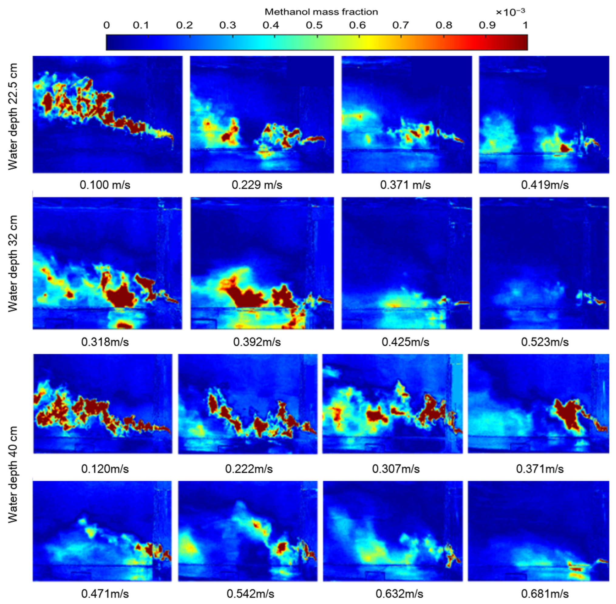
The diffusion pattern of methanol leakage under different water depths and flow velocities is illustrated in Figure 12, where the color scale represents the distribution of methanol mass fraction, visually reflecting the downstream extension range of high-concentration methanol plumes. For the shallow water depth of 22.5 cm and medium depth of 32 cm, the high-concentration methanol cloud stretches a long distance along the flow direction at low velocities, resulting in a larger overall diffusion area. With the increase in flow velocity, turbulent mixing of ambient water is intensified, methanol is diluted rapidly, and both the area and downstream extension length of high-concentration regions decrease simultaneously. When the water depth rises to 40 cm, the dilution capacity of the water body is greatly improved, and the diffusion scale of the high-concentration methanol cloud is obviously smaller than that of the two shallow water groups under identical flow velocity.
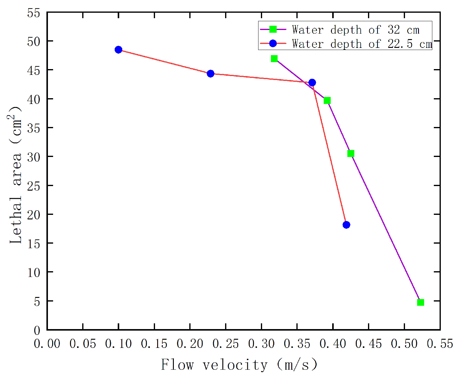
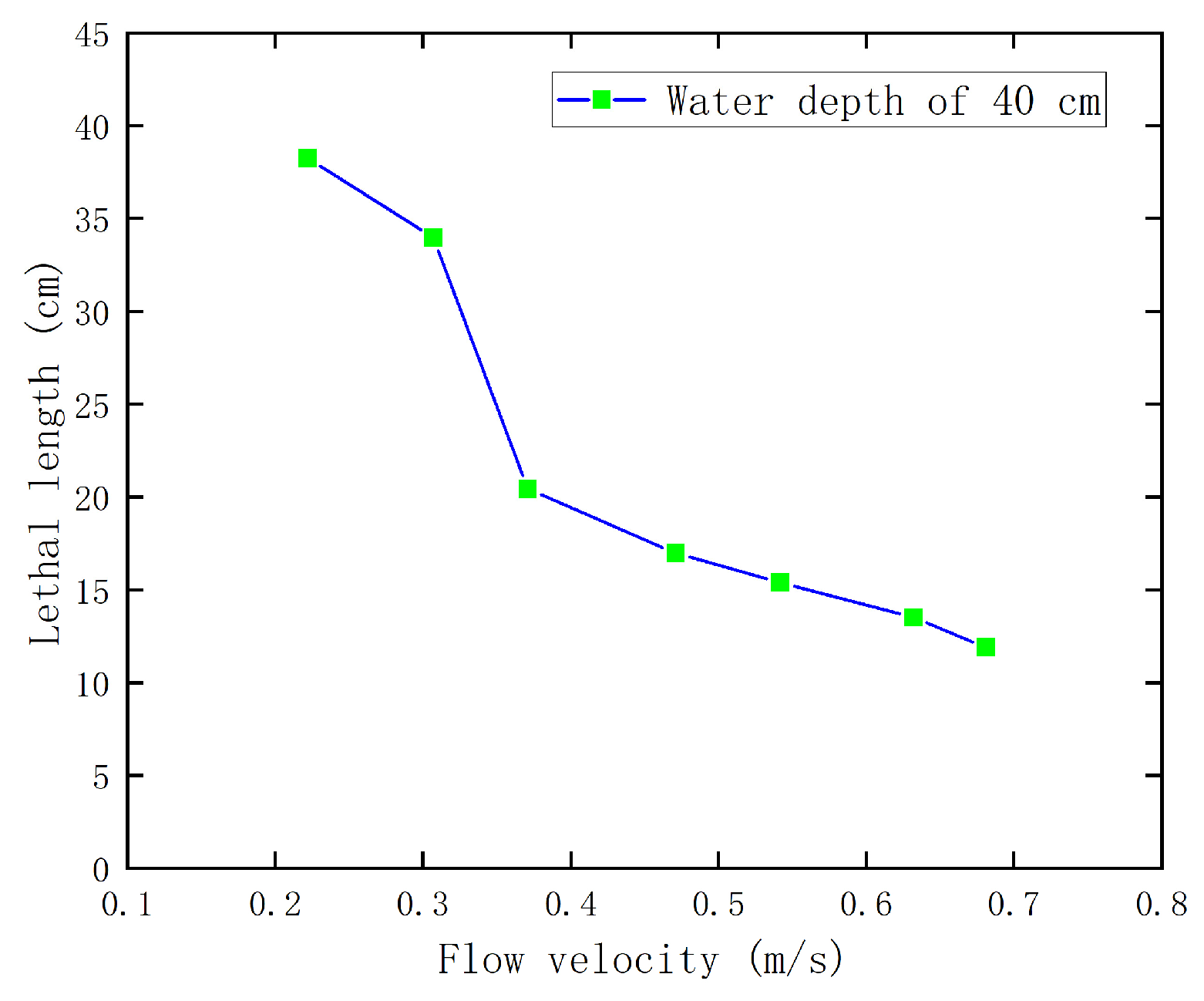
Figure 13 and Figure 14 show the quantitative lethal diffusion length of methanol measured from visualization images. Figure 13 presents the curves of lethal length versus flow velocity under 22.5 cm and 32 cm water depths, and the two curves share similar variation trends: the lethal length remains at a high level of 43–49 cm under low flow velocities, and drops sharply once the flow velocity exceeds 0.35 m/s. At the same flow rate, the lethal diffusion length of 32 cm water depth is always longer than that of 22.5 cm, and its critical velocity for abrupt decline is higher. The curve of 40 cm water depth is displayed in Figure 14, which has no steep mutation segment, and the lethal length decreases gently and continuously with rising flow velocity. The maximum lethal length is only 38 cm at the low velocity of 0.2 m/s, much lower than that of shallow water groups; as the flow velocity increases from 0.2 m/s to 0.68 m/s, the lethal length gradually reduces from 38 cm to 12 cm. Comparative analysis of all working conditions indicates that deeper water possesses stronger dilution buffering capacity, leading to a shorter overall lethal diffusion length of methanol at the same flow velocity. Higher flow velocity enhances turbulent dilution and drastically shrinks the high-concentration lethal zone.
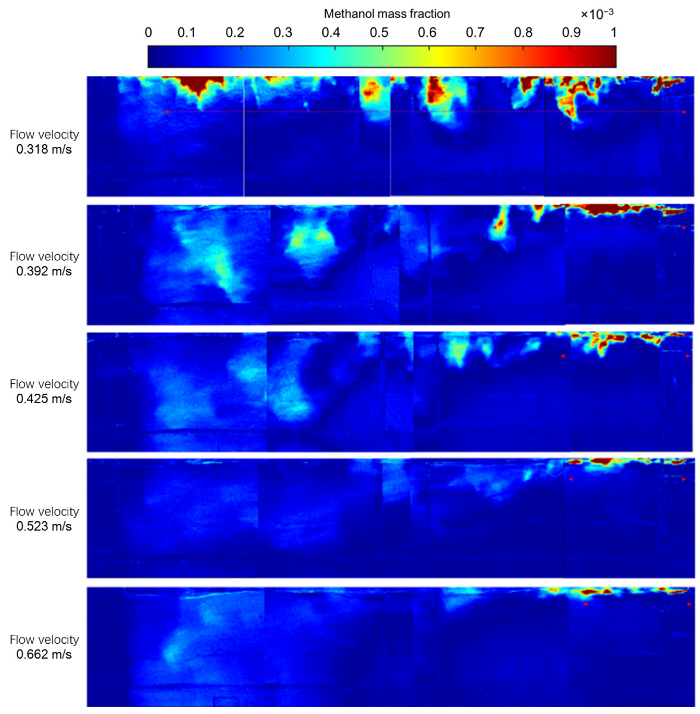
Figure 15 shows methanol mass fraction contours of surface leakage at a fixed water depth of 32 cm and a leak flow rate of 86.18 mL/min. Methanol from surface release spreads horizontally along the water surface, and only a small fraction is entrained underwater by turbulence, with high-concentration plumes limited to a thin surface layer. The red lethal zone extends farthest at low flow velocity; stronger turbulent mixing under higher flow rates continuously reduces the coverage of high-concentration methanol.
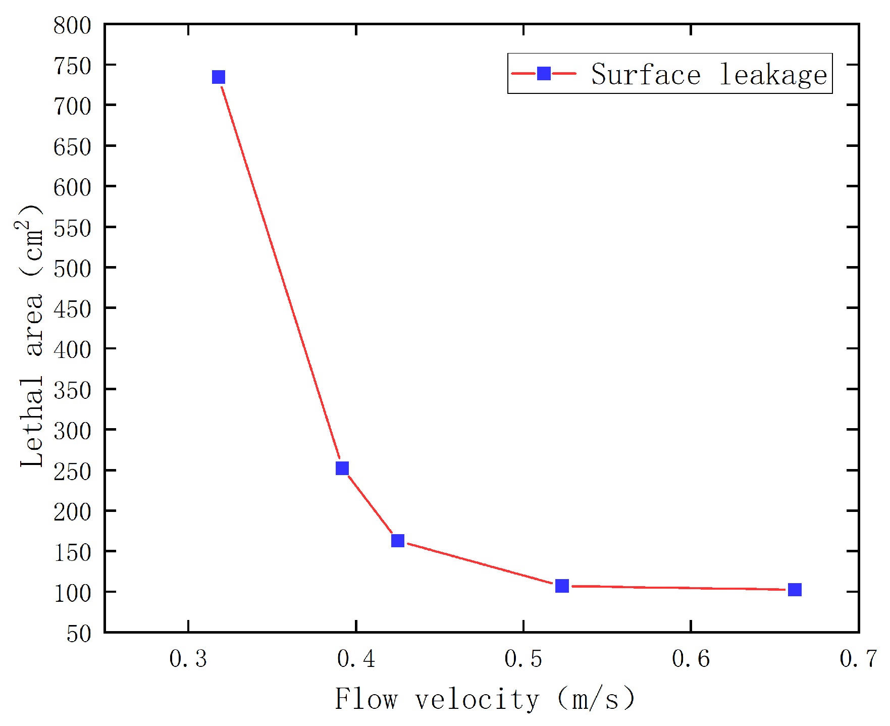
Figure 16 presents the quantitative curve of lethal area extracted from contour data. The lethal area decreases in two distinct stages with rising flow velocity. It reaches a maximum value of 735 cm2 at 0.318 m/s, and then drops sharply to 255 cm2 when velocity rises to 0.4 m/s. The decay slows down above 0.4 m/s, with lethal areas of 165 cm2, 108 cm2 and 102 cm2 at 0.425 m/s, 0.523 m/s and 0.662 m/s, which gradually stabilize at high velocities. Without vertical water buffer for surface leakage, the lethal area is more sensitive to flow dilution, showing a much larger shrinkage range than bottom leakage under increasing flow velocity.

3.2. Effect of Leak Velocity and Water Depth

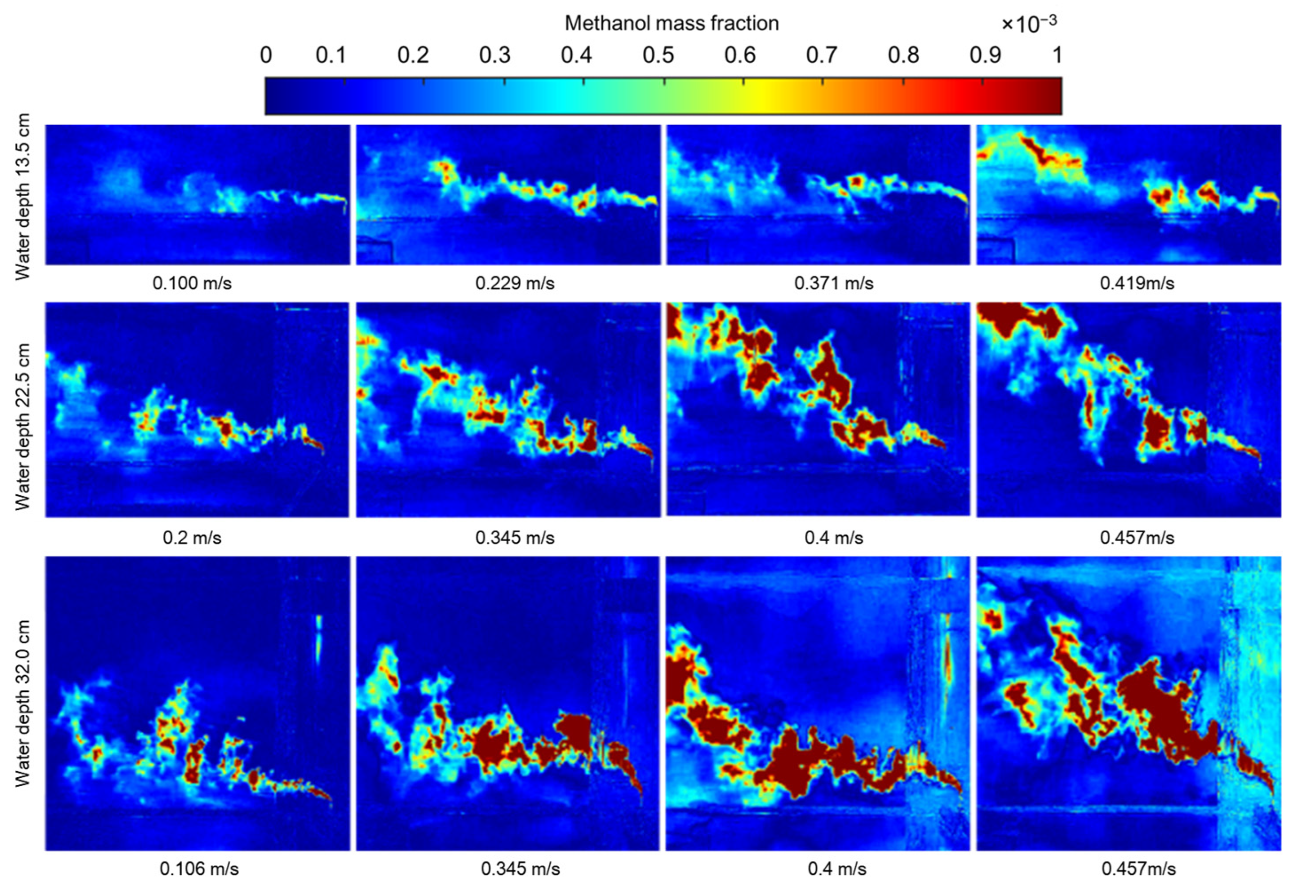
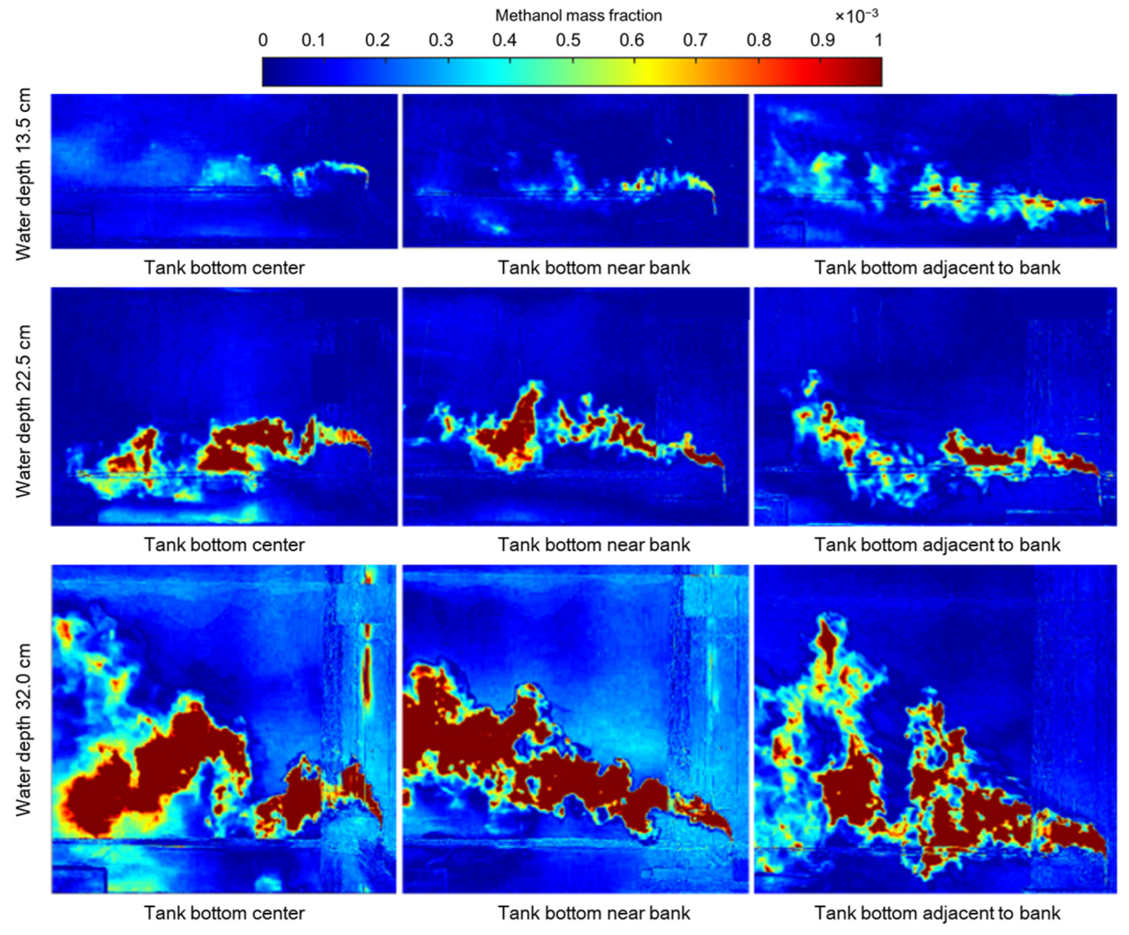
Figure 17 illustrates the mass fraction distribution of methanol plumes from underwater bottom leakage under diverse water depths and leak exit velocities, where the color gradient quantifies methanol concentration and visually characterizes the shape and coverage of high-concentration lethal zones. The water bulk flow velocity was fixed at 0.1 m/s, and leak exit velocities of 0.2 m/s and 0.4 m/s correspond to volumetric flow rates of 37.7 mL/min and 75.4 mL/min, respectively. Shallower water produces a steeper vertical velocity gradient and stronger turbulent mixing. For the 13.5 cm shallow water depth, only the vicinity of the leakage point reaches the lethal mass fraction threshold of 8 × 10⁻⁴. Higher leak exit velocity delivers larger initial momentum to methanol jets, which expands the horizontal lethal coverage and accelerates vertical diffusion toward the water surface. Meanwhile, the larger total methanol input generates a higher concentration gradient and enhances molecular diffusion, further enlarging the overall lethal area.
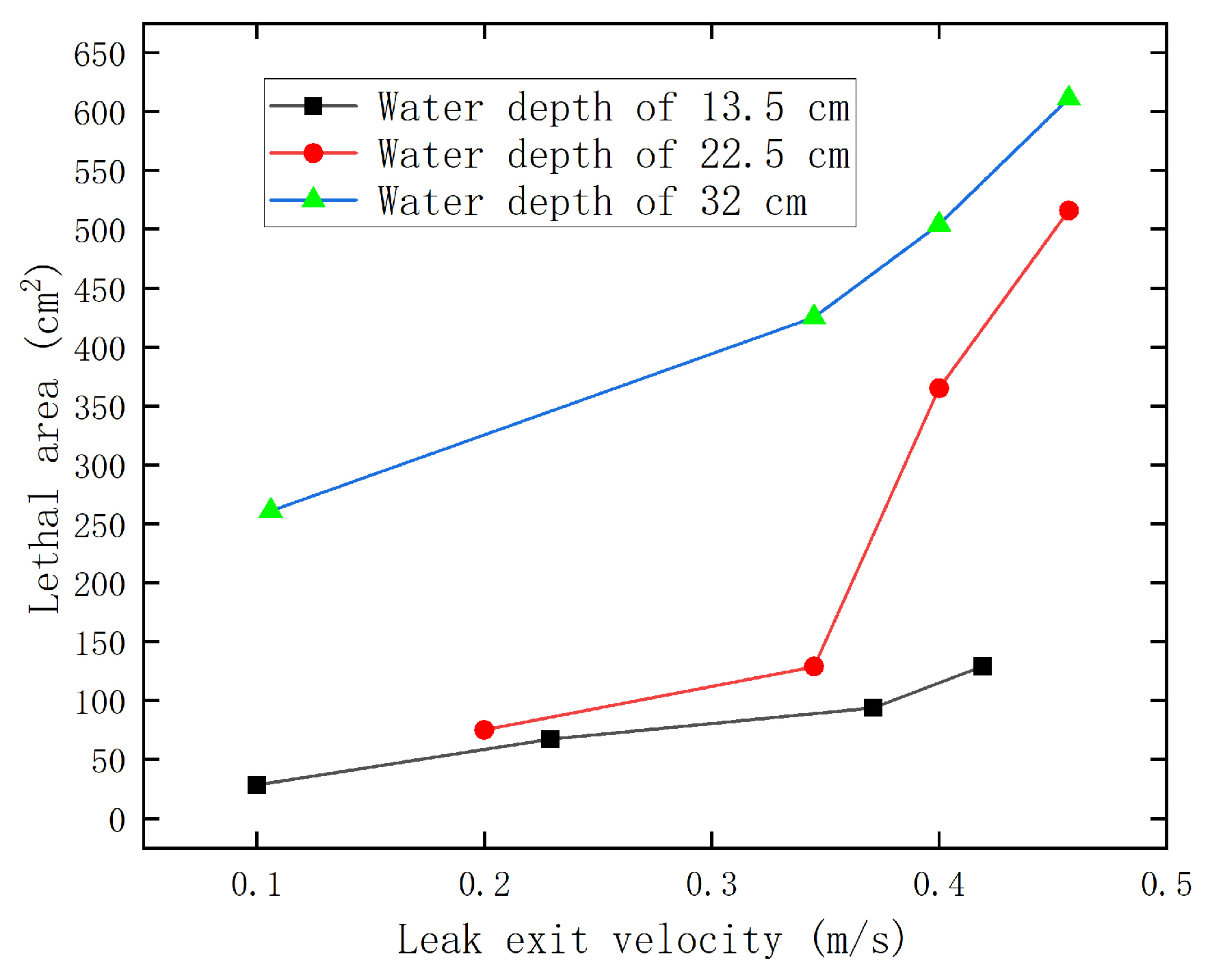
Figure 18 presents the quantitative relationship between lethal zone area and leak exit velocity calculated from the contour images in Figure 11. The lethal area rises monotonously with the increase in leak velocity under all three water depths (13.5 cm, 22.5 cm and 32 cm), and the lethal area follows the order of 32 cm > 22.5 cm > 13.5 cm at identical leakage rates. At the leak velocity of 0.1 m/s, the lethal areas for 13.5 cm, 22.5 cm and 32 cm water depths are approximately 30 cm2, 78 cm2 and 265 cm2, respectively. When the leak velocity increases to around 0.42 m/s, the lethal areas reach 130 cm2, 520 cm2 and 615 cm2, and the numerical gap between groups widens continuously with rising leak velocity. The curve of 13.5 cm shallow water depth grows gently with an extremely low increment throughout the test range. For the 22.5 cm water depth, the slope increases sharply once the leak velocity exceeds 0.35 m/s, leading to explosive expansion of the lethal area. The 32 cm depth curve maintains a steep nearly linear growth trend, and its lethal area is markedly larger than the other two groups at all tested velocities. Intense turbulent dilution in shallow water restrains the expansion of high-concentration plumes. In deeper water, vertical flow confinement is weakened, allowing methanol jet momentum to drive sufficient horizontal and vertical spreading, which eventually forms a much larger lethal area under the same leak velocity condition.

3.3. Effect of Leak Location

Figure 19 presents the methanol mass fraction contour distributions under a fixed leak exit velocity of 0.4 m/s, with three leakage positions set at tank bottom center, near the bank and adjacent to the bank, respectively. The visualized concentration fields clearly reveal that the side bank boundary alters the diffusion pattern of methanol plumes. For center leakage, methanol spreads uniformly in all directions without lateral wall confinement. When leakage occurs near or adjacent to the bank, the single side wall restricts lateral diffusion space, intensifies turbulence generated by flow-bank interaction, and forces high-concentration methanol to transport downstream along the bank side. At identical leakage positions, deeper water yields a far wider coverage of high-concentration methanol plumes. The shallow water depth of 13.5 cm produces the minimum lethal zone throughout tests, while the red high-concentration lethal area under 32 cm water depth greatly exceeds the other two depth groups.
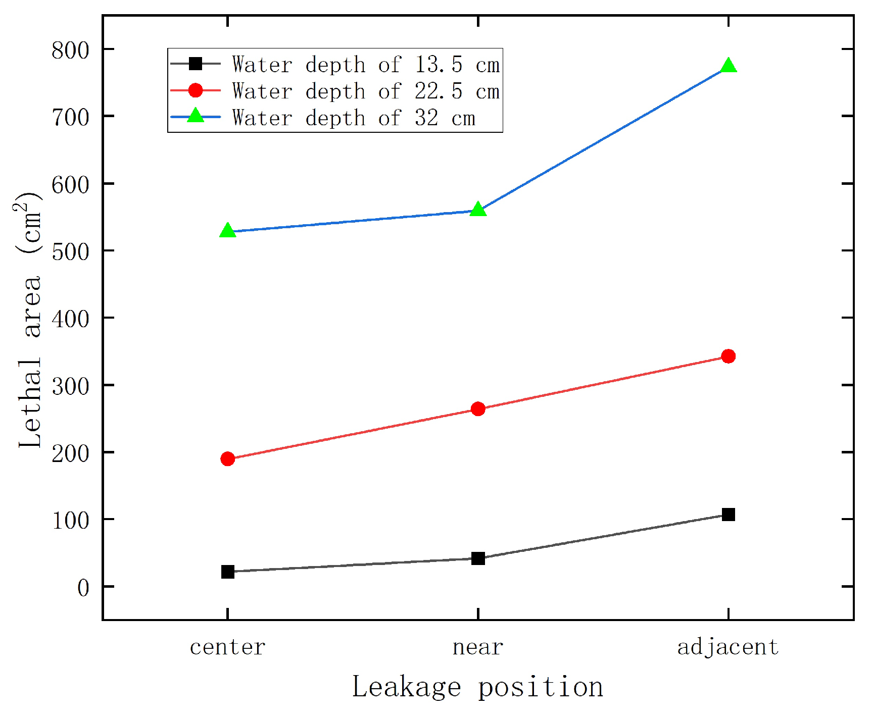
Figure 20 quantifies the lethal zone area extracted from contour images in Figure 13. For all test groups, the lethal area follows the rule of tank bottom center < near bank < adjacent to the bank, and under the same leakage position, the lethal area ranks as 32 cm > 22.5 cm > 13.5 cm with obvious numerical differences. At the center leakage position, the lethal areas of 13.5 cm, 22.5 cm and 32 cm water depths are approximately 25 cm2, 195 cm2 and 530 cm2. When the leakage position shifts to the location adjacent to the bank, the lethal areas increase to 110 cm2, 345 cm2 and 775 cm2, correspondingly. In terms of growth amplitude, the three curves of 13.5 cm shallow water stay at low values with mild increments from the center to the bank; the curve of 22.5 cm depth rises steadily at a constant slope; and the 32 cm depth curve shows the most prominent growth, with a nearly 46% increase in lethal area when leakage moves from the tank center to bank-adjacent positions. The bank boundary blocks lateral dilution of methanol, constrains fluid accumulation on one side and prolongs the residence time of high-concentration methanol. Larger water depth expands the vertical diffusion space and weakens the dilution effect of bottom turbulence. The combined effects of the two factors maximize the lethal coverage area under the condition of bank-adjacent leakage and deep water.
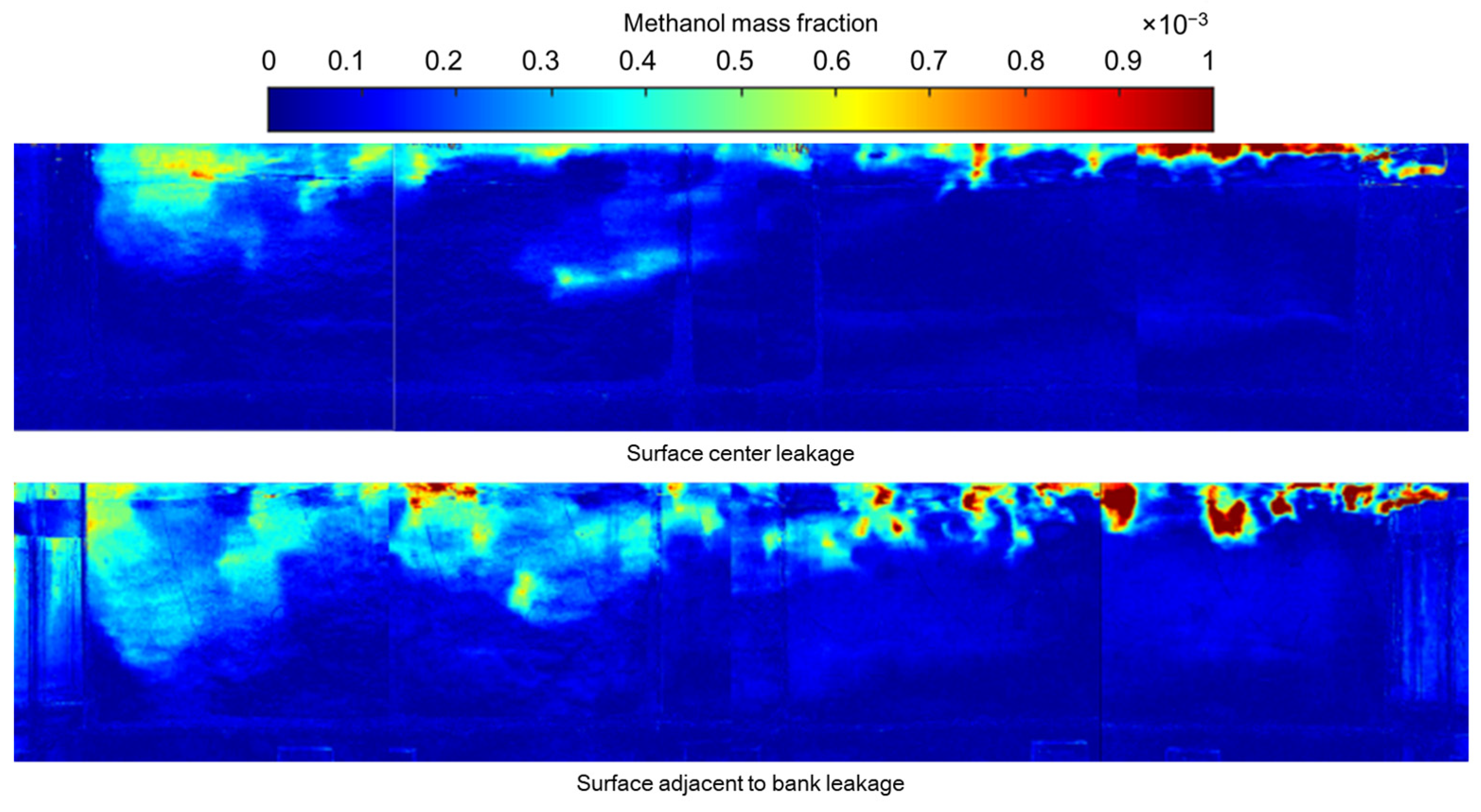
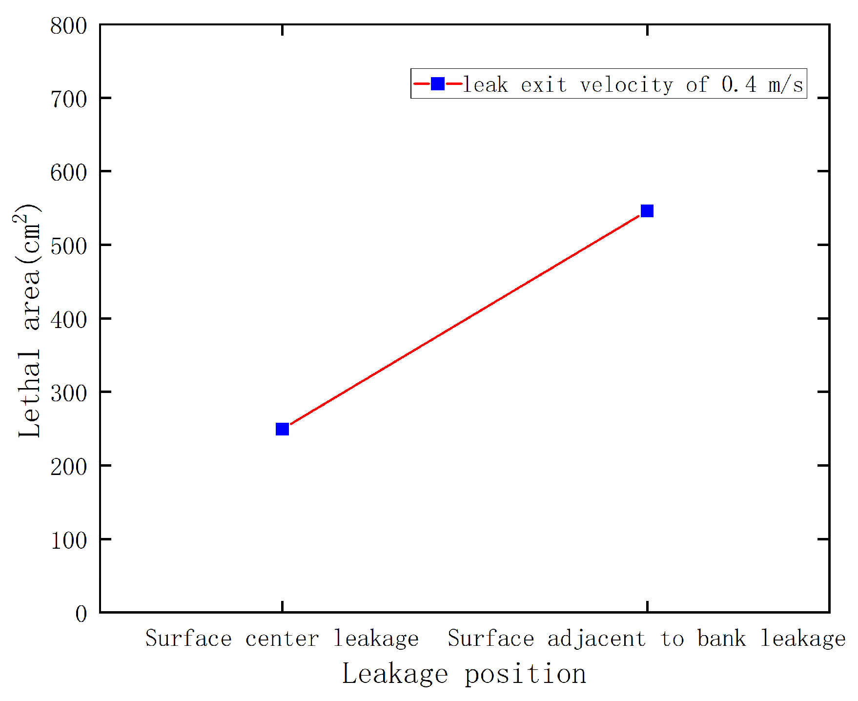
Figure 21 displays methanol mass fraction contours of two surface leakage positions under a fixed water depth of 0.32 m, a flow velocity of 0.318 m/s and a leak velocity of 0.457 m/s. Methanol diffuses more evenly for surface center leakage without lateral restriction, while surface leakage adjacent to the bank accumulates high-concentration methanol along the side wall, forming a broader lethal zone.
Figure 22 quantifies the lethal area extracted from contour images. The lethal area rises sharply when the leak point moves closer to the bank. The lethal area is about 250 cm2 for surface center leakage and increases to 550 cm2 for bank-adjacent surface leakage. The stable flow and limited diffusion space near the bank cause methanol accumulation and expand the lethal coverage.

4. Discussion of Experimental Limitations and Scaling Effects

This study was performed in a laboratory-scale, recirculating open-channel flume, which inevitably introduces limitations when extrapolating results to natural river systems. Although the experimental design enables controlled investigation of key governing parameters, several scale- and geometry-related constraints should be considered.
First, the closed-loop circulation system may introduce weak recirculation of tracer water. While each experiment was limited to a short duration (t = 5 s) to minimize re-entrainment effects, residual feedback within the system cannot be completely excluded. Nevertheless, its influence is considered minor for the early stage plume evolution analyzed in this study.
Second, the experimental flume features a smooth-bed, rectangular cross-section, which simplifies the highly heterogeneous conditions of natural rivers. Real rivers exhibit complex bathymetry, spatially variable roughness, vegetation, and irregular bank morphology, all of which can significantly modify secondary flows and turbulent structures. In contrast, the present configuration yields more idealized and stable boundary conditions, particularly near the banks. As a result, boundary-induced turbulence and flow heterogeneity may be under-represented.
Third, although the Reynolds and Froude numbers confirm fully turbulent, subcritical flow conditions, the absolute magnitudes remain lower than those typically observed in field-scale rivers. Consequently, turbulence characteristics, mixing length scales, and dispersion rates are inherently scale dependent. These differences may affect the quantitative evolution of plume spreading, particularly transverse mixing efficiency and downstream decay rates.
Despite these limitations, the observed trends are physically consistent with established open-channel mixing theory. The influence of flow velocity, water depth, leak rate, and leakage location on plume evolution is robust and qualitatively transferable to natural river systems within the parameter space investigated in this study. These ranges correspond to fully turbulent, subcritical flows, which are representative of small to medium-sized lowland rivers with moderate flow velocities (typically 0.1–0.7 m/s) and shallow to moderate depths (0.1–0.4 m). In particular, the identified mechanisms—velocity-enhanced dilution, depth-controlled mixing capacity, and bank-induced confinement—are expected to remain valid under field conditions where the flow regime falls within similar Reynolds and Froude number ranges. However, for large deep rivers with significantly higher Reynolds numbers (Re > 106) or steep mountainous streams with supercritical flows (Fr > 1), the quantitative trends observed here may not be directly applicable, and further experimental or numerical validation would be required.
However, quantitative metrics such as lethal zone length and area should be interpreted as system-specific results rather than direct field predictions. For practical applications, these results are best used as mechanistic guidance for hazard assessment and emergency response strategy development, while site-specific modeling or field calibration is required for accurate risk quantification.
Future work should focus on dynamic similarity-based scaling, larger-scale experimental validation, or coupled CFD–experimental frameworks to improve transferability to real river environments.

5. Conclusions

This study experimentally investigated the leakage and diffusion behavior of methanol in a controlled open-channel flow environment, with emphasis on the effects of water flow velocity, water depth, leak rate, and leakage location. Based on image-based concentration reconstruction and quantitative analysis of high-concentration (lethal threshold) zones, the following conclusions can be drawn:
(1)
The downstream transport and spatial extent of methanol plumes are strongly influenced by ambient flow velocity. Increasing flow velocity enhances advective transport and turbulent mixing, leading to a systematic reduction in the downstream extension length and overall size of high-concentration regions.
(2)
Water depth plays a significant role in modulating dilution capacity and vertical mixing behavior. Under deeper water conditions, plume structures exhibit larger spatial persistence, while shallower water enhances dilution and restricts the development of high-concentration zones due to stronger relative boundary effects.
(3)
Leak rate affects both the magnitude and spatial distribution of methanol concentration. Higher leakage rates increase local concentration levels and promote the expansion of high-concentration regions, particularly in the near-field zone, due to increased momentum input and mass loading.
(4)
Leakage location significantly alters plume morphology. Near-bank leakage leads to more confined lateral spreading due to boundary constraints, whereas central leakage allows more symmetric dispersion. These effects become more pronounced under higher water depth conditions.
Overall, the results demonstrate that methanol plume evolution in open-channel flow is governed by the coupled interaction of advection, turbulent mixing, and boundary confinement. The observed behaviors are consistent across the tested parameter space and provide experimental evidence for understanding key controlling mechanisms of soluble pollutant transport in simplified open-channel systems.

Author Contributions

Conceptualization, C.N. and R.Z.; methodology, W.W.; validation, Q.X.; formal analysis, C.N.; investigation, R.Z.; resources, W.W.; data curation, L.L.; writing—original draft preparation, Q.X.; writing—review and editing, all authors; visualization, C.N.; supervision, R.Z.; project administration, W.W.; All authors have read and agreed to the published version of the manuscript.

Funding

This research was funded by the Major Program of the National Natural Science Foundation of China (Grant No. 52192623) and the National Natural Science Foundation of China (Grant No. 52006242).

Data Availability Statement

The data presented in this study are available on request from the corresponding author (wangji@cup.edu.cn).

Conflicts of Interest

The authors declare no conflicts of interest.

References

  1. Kim, S.; Kim, H.; Lee, J.; Cho, K.H. Chemical accidents in freshwater: Development of forecasting system for drinking water resources. J. Hazard. Mater. 2022, 432, 128714. [Google Scholar] [CrossRef] [Scilit] [PubMed]
  2. McCready, D.; Williams, J.B. A simplified approach to evaluate human and aquatic exposure to a chemical spilled in a river. J. Hazard. Mater. 2011, 193, 225–232. [Google Scholar] [CrossRef] [Scilit] [PubMed]
  3. Bencala, K.E.; Walters, R.A. Simulation of Solute Transport in a Mountain Pool-and-Riffle Stream: A Transient Storage Model. Water Resour. Res. 1983, 19, 718–724. [Google Scholar] [CrossRef] [Scilit]
  4. Fischer, H.B. Longitudinal Dispersion and Turbulent Mixing in Open-Channel Flow. Annu. Rev. Fluid Mech. 1973, 5, 59–78. [Google Scholar] [CrossRef] [Scilit]
  5. Kaviraj, A.; Bhunia, F.; Saha, N.C. Toxicity of Methanol to Fish, Crustacean, Oligochaete Worm, and Aquatic Ecosystem. Int. J. Toxicol. 2004, 23, 55–63. [Google Scholar] [CrossRef] [Scilit] [PubMed]
  6. Enrique, M. Methanol Safe Handling Manual; Methanol Institute: Washington, DC, USA, 2013; Available online: https://www.methanol.org/wp-content/uploads/2017/03/Safe-Handling-Manual.pdf (accessed on 25 March 2026).
  7. Mackay, D.; Shiu, W.Y.; Ma, K.C.; Lee, S.C. Handbook of Physical-Chemical Properties and Environmental Fate for Organic Chemicals; CRC Press: Boca Raton, FL, USA, 2006. [Google Scholar] [CrossRef] [Scilit]
  8. Klöpffer, W.; Rippen, G.; Frische, R. Physicochemical properties as useful tools for predicting the environmental fate of organic chemicals. Ecotoxicol. Environ. Saf. 1982, 6, 294–301. [Google Scholar] [CrossRef] [Scilit] [PubMed]
  9. Shin, J.; Seo, I.W.; Baek, D. Longitudinal and transverse dispersion coefficients of 2D contaminant transport model for mixing analysis in open channels. J. Hydrol. 2020, 583, 124302. [Google Scholar] [CrossRef] [Scilit]
  10. Kim, J.S.; Baek, D.; Park, I. Evaluating the Impact of Turbulence Closure Models on Solute Transport Simulations in Meandering Open Channels. Appl. Sci. 2020, 10, 2769. [Google Scholar] [CrossRef] [Scilit]
  11. Boxall, J.B.; Guymer, I. Analysis and Prediction of Transverse Mixing in Natural Channels. J. Hydraul. Eng. 2003, 129, 129–139. [Google Scholar] [CrossRef] [Scilit]
  12. Shiono, K.; Feng, T. Turbulence Measurements of Dye Concentration and Effects of Secondary Flow on Distribution in Open Channel Flows. J. Hydraul. Eng. 2003, 129, 373–382. [Google Scholar] [CrossRef] [Scilit]
  13. Pouchoulin, S.; Le Coz, J.; Mignot, E.; Gond, L.; Riviere, N. Predicting Transverse Mixing Efficiency Downstream of a River Confluence. Water Resour. Res. 2020, 56, e2019WR026367. [Google Scholar] [CrossRef] [Scilit]
  14. Guo, J.; Jiang, W.; Chen, G.; Li, Z.; Alharbi, N.S.; Wakeel, M. Solute dispersion in an open channel turbulent flow: Solution by a generalized model. J. Hydrol. 2022, 604, 127239. [Google Scholar] [CrossRef] [Scilit]
  15. Runkel, R.L. A New Metric for Determining the Importance of Transient Storage. J. N. Am. Benthol. Soc. 2002, 21, 529–543. [Google Scholar] [CrossRef] [Scilit] [PubMed]
  16. Weill, S.; Mazzia, A.; Putti, M.; Paniconi, C. Coupling water flow and solute transport into a physically-based surface–subsurface hydrological model. Adv. Water Resour. 2011, 34, 128–136. [Google Scholar] [CrossRef] [Scilit]
  17. Roberts, P.J.W.; Ferrier, A.; Daviero, G. Mixing in inclined dense jets. J. Hydraul. Eng. 1997, 123, 693–699. [Google Scholar] [CrossRef] [Scilit]
  18. Mossa, M.; Davies, P.A. Some Aspects of Turbulent Mixing of Jets in the Marine Environment. Water 2018, 10, 522. [Google Scholar] [CrossRef] [Scilit]
  19. Chen, F.; MacDonald, D.G. Role of Mixing in the Structure and Evolution of a Buoyant Discharge Plume. J. Geophys. Res. Oceans 2006, 111, C11020. [Google Scholar] [CrossRef] [Scilit]
  20. Crimaldi, J.P. Planar Laser Induced Fluorescence in Aqueous Flows. Exp. Fluids 2008, 44, 851–863. [Google Scholar] [CrossRef] [Scilit]
  21. Albayrak, I.; Lemmin, U. Secondary Currents and Corresponding Surface Velocity Patterns in a Turbulent Open-Channel Flow over a Rough Bed. J. Hydraul. Eng. 2011, 137, 1566–1575. [Google Scholar] [CrossRef] [Scilit]
  22. Gualtieri, C.; Savino, A.; Veltri, P. Transverse mixing in a trapezoidal compound open channel. J. Hydrodyn. Ser. B 2008, 20, 645–649. [Google Scholar] [CrossRef] [Scilit]
  23. Eidelman, A.; Elperin, T.; Kleeorin, N.; Hazak, G.; Rogachevskii, I.; Sadot, O.; Sapir-Katiraie, I. Mixing at the external boundary of a submerged turbulent jet. Phys. Rev. E 2009, 79, 026311. [Google Scholar] [CrossRef] [Scilit] [PubMed]
  24. Khaldi, N.; Marzouk, S.; Mhiri, H.; Bournot, P. Distribution characteristics of pollutant transport in a turbulent two-phase flow. Environ. Sci. Pollut. Res. 2015, 22, 6349–6358. [Google Scholar] [CrossRef] [Scilit] [PubMed]
  25. Blocken, B. Computational Fluid Dynamics for Urban Physics: Importance, Scales, Possibilities, Limitations and Ten Tips and Tricks Towards Accurate and Reliable Simulations. Build. Environ. 2015, 91, 219–245. [Google Scholar] [CrossRef] [Scilit]
  26. Meselhe, E.A.; Sotiropoulos, F. Three-dimensional numerical model for open-channels with free-surface variations. J. Hydraul. Res. 2000, 38, 115–121. [Google Scholar] [CrossRef] [Scilit]
  27. Adrian, R.J. Particle-Imaging Techniques for Experimental Fluid Mechanics. Annu. Rev. Fluid Mech. 1991, 23, 261–304. [Google Scholar] [CrossRef]
  28. Raffel, M.; Willert, C.E.; Wereley, S.; Kompenhans, J. Particle Image Velocimetry: A Practical Guide; Springer: Berlin/Heidelberg, Germany, 2007. [Google Scholar] [CrossRef] [Scilit]
  29. Houcine, I.; Vivier, H.; Plasari, E.; David, R. Planar Laser Induced Fluorescence Technique for Measurement of Concentration Fields in Continuous Stirred Tank Reactors. Exp. Fluids 1996, 22, 95–102. [Google Scholar] [CrossRef] [Scilit]
  30. van Meerkerk, M.; Poelma, C.; Westerweel, J. Scanning stereo-PLIF method for free surface measurements in large 3D domains. Exp. Fluids 2020, 61, 19. [Google Scholar] [CrossRef] [Scilit]
  31. Feng, L.; Yang, L.; Li, Y.; Zhang, J. Mixing characterization in different helically coiled configurations by laser-induced fluorescence. Exp. Fluids 2020, 61, 203. [Google Scholar] [CrossRef] [Scilit]
  32. Massaro, D.; Di Felice, F.; Felli, M.; Romano, G.P. Mass and momentum transport in the near field of swirling turbulent jets. Effect of swirl rate. Int. J. Heat Fluid Flow 2020, 83, 108539. [Google Scholar] [CrossRef] [Scilit]
  33. Craske, J.; Davies Wykes, M.S. The entrainment and energetics of turbulent plumes in a confined space. J. Fluid Mech. 2020, 883, A2. [Google Scholar] [CrossRef] [Scilit]
  34. He, Z.; Zhang, W.; Jiang, H.; Zhao, L.; Han, X. Dynamic Interaction and Mixing of Two Turbulent Forced Plumes in Linearly Stratified Ambience. J. Hydraul. Eng. 2018, 144, 04018065. [Google Scholar] [CrossRef] [Scilit]
  35. Lin, L.K.; Niu, Q.Q.; Li, Y. Camera calibration method based on checkerboard. Comput. Technol. Dev. 2023, 33, 101–106. [Google Scholar] [CrossRef]
  36. Zhang, Z.Y. A flexible new technique for camera calibration. IEEE Trans. Pattern Anal. Mach. Intell. 2000, 22, 1330–1334. [Google Scholar] [CrossRef] [Scilit]
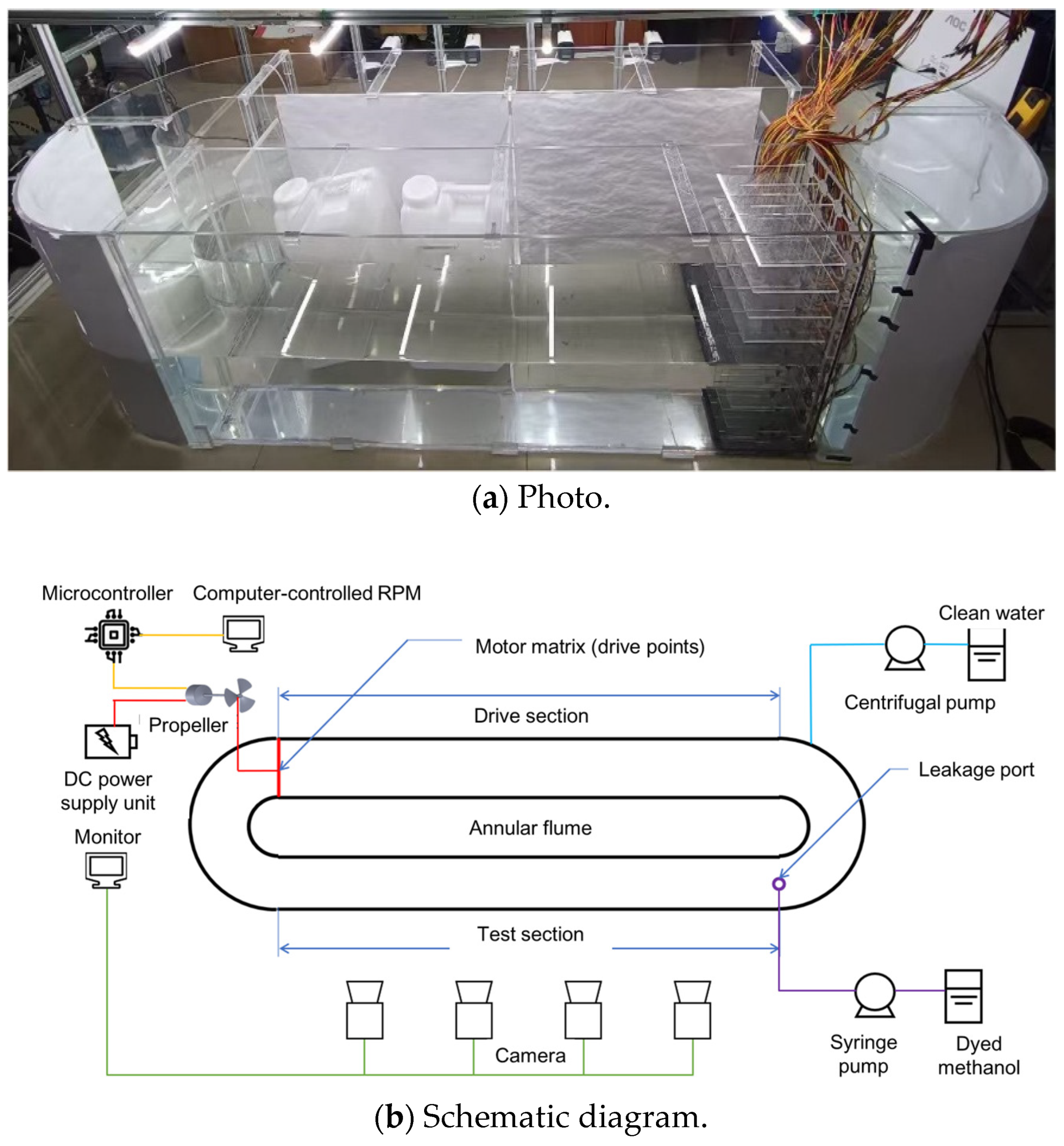
Figure 1. Experimental system.
Pollutants 06 00040 g001
Figure 2. Methanol concentration calibration experiment setup.
Pollutants 06 00040 g002
Figure 3. Images for several methanol concentration solutions.
Pollutants 06 00040 g003
Figure 4. Methanol concentration–greyscale value correlation curve.
Pollutants 06 00040 g004
Figure 5. Chessboard image.
Pollutants 06 00040 g005
Figure 6. Original images.
Pollutants 06 00040 g006
Figure 7. Corrected images.
Pollutants 06 00040 g007
Figure 8. Image processing.
Pollutants 06 00040 g008
Figure 9. Comparison between measured sampling concentration percentages and image greyscale back-calculated concentration percentages at four monitoring points.
Pollutants 06 00040 g009
Figure 10. Instantaneous morphology of methanol leakage plume in the visual experiment (colored original image); ①, ②, ③ and ④ indicate the locations of monitoring points.
Pollutants 06 00040 g010
Figure 11. Greyscale-converted version of the methanol leakage plume shown in Figure 1 for concentration back-calculation; ①, ②, ③ and ④ indicate the locations of monitoring points.
Pollutants 06 00040 g011
Figure 12. Methanol diffusion for various water velocities (leak from tank bottom).
Pollutants 06 00040 g012
Figure 13. Lethal area vs. flow velocity (22.5 cm and 32 cm water depth).
Pollutants 06 00040 g013
Figure 14. Lethal length vs. flow velocity (40 cm water depth).
Pollutants 06 00040 g014
Figure 15. Methanol diffusion for various water flow velocities (leak from water surface middle zone).
Pollutants 06 00040 g015
Figure 16. Lethal area versus flow velocity under surface leakage.
Pollutants 06 00040 g016
Figure 17. Methanol diffusion for various leak velocities (leak from the tank bottom with water flow velocity of 0.1 m/s).
Pollutants 06 00040 g017
Figure 18. Lethal area vs. leak exit velocity at water depths of 13.5 cm, 22.5 cm and 32 cm.
Pollutants 06 00040 g018
Figure 19. Methanol diffusion for various leak locations (leak from the tank bottom).
Pollutants 06 00040 g019
Figure 20. Lethal area versus leakage position at water depths of 13.5 cm, 22.5 cm and 32 cm.
Pollutants 06 00040 g020
Figure 21. Methanol diffusion for various leak locations from water surface.
Pollutants 06 00040 g021
Figure 22. Lethal area vs. surface leakage position (leak exit velocity = 0.4 m/s).
Pollutants 06 00040 g022
Table 1. Summary of the calculated ranges of Re and Fr for all experimental conditions.
Water Depth (m)Flow Velocity (m/s)ReFr
0.1350.29639,7220.257
0.2250.10–0.41922,366–93,7120.067–0.282
0.320.318–0.523101,152–166,3620.179–0.295
0.400.12–0.68147,713–270,7770.061–0.344
Table 2. Experimental conditions.
ParametersExperimental Conditions
Leak locationChannel bottom (center, near bank, adjacent to bank)
Water surface (center, near bank, adjacent to bank)
Leak flow rate (mL/min)20, 37.7, 56.55, 65, 75.4, 86.18
Water flow velocity (m/s)0.1, 0.229, 0.419, 0.318, 0.392, 0.425, 0.523, 0.12, 0.222, 0.307, 0.371, 0.471, 0.542, 0.632, 0.681, 0.2, 0.345, 0.4, 0.457, 0.106
Water depth (m)0.135, 0.225, 0.32, 0.4
Table 3. Coefficients of image calibration equations.
CoefficientsOverhead CameraSide-View Camera
TD195.70706151.2208
TD279.00325128.16395
Yb0.005440.00425
A1−0.00206−0.00294
A2−0.00368−0.00199
τ11.24816.7663
τ281.43055121.5813
Disclaimer/Publisher’s Note: The statements, opinions and data contained in all publications are solely those of the individual author(s) and contributor(s) and not of MDPI and/or the editor(s). MDPI and/or the editor(s) disclaim responsibility for any injury to people or property resulting from any ideas, methods, instructions or products referred to in the content.