Hybrid Cycle Slip Detection Method for Smartphone Global Navigation Satellite System ^†

Abstract

The main roadblock to precise Smartphone GNSS positioning is erroneous carrier phase data which is highly prone to cycle slips (CSs). There is a dearth of research on cycle slip detection and repair (CSDR) methods for Smartphone GNSS. Existing literature on CSDR methods is based on phase data captured by professional-grade receivers. These methods can be broadly categorized into two groups: (1) Geometry-Free CSDR (GF-CSDR) and (2) Geometry-Based CSDR (GB-CSDR). GF-CSDR methods rely on individual satellite measurements, whereas the GB-CSDR technique considers the whole satellite–receiver geometry. This paper proposes a real-time single-frequency CSDR method combining both GF and GB-CSDR. Experimental results are presented for a static and a kinematic smartphone dataset. It is shown that although reliable CS detection is possible for Smartphone GNSS, CS repair reliability is limited due to the carrier phase precision quality.

1. Introduction

High-precision positioning in smartphones remains elusive because of poor measurement quality. Single-frequency Precise Point Positioning (PPP) on smartphones exemplifies this trend. The main challenge with Smartphone GNSS is the low-cost chipset and antenna, which leads to high pseudorange noise, and the carrier phase being subject to frequent cycle slips [1], especially when the receiver is moving.

Most Smartphone PPP implementations reset ambiguity parameters upon detecting CSs and do not attempt to repair them. This degrades PPP performance. Even a single CS can weaken the geometry and may lead to poorer positioning and longer ambiguity convergence time. Therefore, CSDR is critical for reliable Smartphone PPP performance.

GNSS Cycle Slip detection and repair (CSDR) techniques can be categorized into two primary approaches: (1) Geometry-Free CSDR methods (GF-CSDR) and (2) Geometry-Based CSDR methods (GB-CSDR). The GF-CSDR methods rely on individual satellite measurements or their linear combinations to detect CSs while GB-CSDR techniques use multiple channels and satellite–receiver geometry to improve the precision of CSDR.

GF-CSDR methods emerged in the late 1980s [2,3,4,5]. The most important GF-CSD testing quantities are the following: (1) the Geometry Free (GF) combination, or phase–ionosphere–residual combination, (2) Melbourne–Wubenna (MW) combination, and (3) Phase-minus-Code (PMC) combination. The GF and MW combinations require dual-frequency data, whereas the PMC combination only needs single-frequency data.

The renowned Turboedit method was introduced in [3]. The GF and MW combinations were used for GF-CSDR in relative/differential positioning, with observables being double-differenced in [6,7]. In [4] a Kalman Filter (KF) was proposed to filter the GF and MW combinations to estimate the exact value of the slip, after detecting and approximating an initial value for the slip using a time-differenced PMC combination. In [8], time-differenced Phase-minus-Code (PMC), along with polynomial fitting, is used to perform CSDR. In [9], a CS-testing quantity termed TECR (total electron content (TEC) rate) was introduced, which is equivalent to a time-differenced GF combination. The TECR and MW combination was used with a “Mean and Sigma computation using sliding window” for CSDR.

The use of Doppler measurement in GF-CSDR is demonstrated in [5,10,11,12]. The testing quantity is equal to the difference in the time-differenced carrier phase (TDCP) and delta-range derived from averaging consecutive epochs of Doppler measurements.

$$testing qty=\left({\Phi }_{k+∆t}-{\Phi }_k\right)-\left({\displaystyle \frac{{\mathrm{D}}_{k+∆t}+{\mathrm{D}}_k}{2}}\right)·∆t=\lambda ·CS+\epsilon$$

(1)

Subtracting the Doppler-derived delta-range from TDCP results in removing the geometry from the testing quantity. The accuracy/preciseness of the CS detection and estimation depends on remaining errors, $\epsilon$, which include the variation in atmospheric delay, satellite orbit bias, multipath, and receiver system noise that should be around a few centimetres when the sampling rate is high, i.e., much less than one cycle. The testing quantity (1) is referred to as the “phase-prediction” method in this paper.

A class of GF-CSDR methods exist which are based on the concept of measurement-based polynomial fitting. A GF-CSDR method based on Bayesian theory is presented in [13]. In [14], piecewise cubic curve fitting is performed on a number of consecutive data using the least squares cubic spline approximation (LS-CSA).

Early Geometry-Based CSDR methods were conceptualized as part of GNSS Quality Control theory [15,16]. These CSDR methods involve performing statistical testing on the phase residuals obtained after estimating a GNSS solution using least-squares or a Kalman Filter. Position estimation implies that the receiver–satellite geometry enters the CSDR model. GB-CSDR methods benefit from the redundancy in the system, which, in the context of CSDR, means that healthy phase measurements also assist in detecting phase measurements affected by cycle slips. GB-CSDR methods can be divided into two groups based on whether or not they time difference consecutive carrier phase measurements.

In [17,18] statistical testing is performed on the Kalman Filter innovation for the performance of CSDR. The papers are based on DGPS/RTK positioning. Similarly [19,20] specifically focus on similar GB-CSDR methods for Precise Point Positioning (PPP). None of these papers implement time-differencing carrier phase measurements.

TDCP residual testing is used in [21,22,23,24,25]. In [22], multi-epoch, multi-frequency TDCP data are used. CS repair is reinforced by using TDCP from previous epochs, for which CSs are absent or have been repaired. A Doppler-derived delta-range is used in the measurement update step, along with TDCP to strengthen statistical testing of single-frequency CSs in [23]. In [24], wide-lane ambiguities are estimated and fixed, and used with the GF combination to perform CSDR for PPP applications. In [25] a GB-CSDR method is introduced for RTK positioning, which uses positional polynomial fitting (PPF) to model user dynamics.

This paper proposes a hybrid CSDR method that uses phase-prediction based GF-CSD to detect and exclude satellites with large cycle slips. It then employs a GB-CSD, which relies on statistical testing of the innovation sequence [16] of TDCP measurements, to detect small cycle slips. The proposed method is built around estimating delta-position (change in receiver position which is equivalent to a discrete estimate of the receiver velocity) along with the size of cycle slips from the delta-ranges derived from the Doppler and carrier phase measurements using a Kalman Filter (KF). Note that in this paper, the terms “delta-range derived from carrier phase” and “TDCP” will be used interchangeably as they refer to the same observable. Once cycle slips are detected and float-valued estimates of their magnitudes are acquired, the most probable corresponding integer values are determined using the Least-Squares Ambiguity Decorrelation Adjustment (LAMBDA) [26] method.

This paper does not implement a PPP algorithm, as neither the cycle slip parameters nor the ambiguities are part of the state vector. Instead, their estimation and resolution are performed in a parallel filter. The proposed CSDR is instantaneous and is based on two epochs of data, though sequential filtering is involved, which improves the CS detection and repair capability.

The paper is organized into the following sections. Section 2 analyzes the Android-based smartphone datasets used in this study. In Section 3, the conventional GF-CSD methods are implemented on smartphone data, and their results are demonstrated. In Section 4, the time-difference functional model used in this study is introduced. Section 5 briefly summarizes the integer ambiguity resolution technique and validation method, along with how it is related to the preciseness of TDCP measurements. A detailed outline of the proposed CSDR method is presented in Section 6. Experimental results are shown in Section 7. The conclusion and future scope are presented in Section 8.

2. Smartphone GNSS Data

Two publicly available datasets were used to test our method. The first was a static rooftop Samsung S20+ dataset labelled “T-A-SIS-01” from the GSA GNSS Raw Measurements Task Force—Measurement Database [27]. The second was a kinematic Google Smartphone Decimeter Challenge 2021 dataset labelled “2021-03-10-US-SVL-1” [28] collected with a Samsung S20 Ultra mounted in a vehicle and driven around the San Francisco Bay Area. Both datasets have a sampling rate of 1 Hz and include a ground truth file generated using the NovAtel SPAN (GNSS + IMU) system. As our method is a single-frequency method, and most Smartphone GNSSs are single-frequency, only L1, E1, and B1I signals are considered.

Figure 1A shows the error in the delta-ranges of carrier phase, Doppler and pseudorange for a single satellite. The standard deviation (SD) of the error series was calculated after omitting outliers larger than three times the median absolute deviation. Since Smartphone GNSS data are prone to large outliers, especially carrier phase, removing outliers before calculating the SD is essential. As expected, the pseudorange delta-range error is significantly larger than that of phase and Doppler. Furthermore, the delta-range errors for the kinematic dataset are worse than those of the static dataset, with the SD approximately twice as large. Noticeably, the preciseness of Doppler-derived delta-range is similar to that of the phase delta-range. Figure 1B shows the delta-range error for all satellites as a function of elevation angle and $C/N_0$. The static data have a consistent error distribution, apart from a few satellites at low elevation angles and low $C/N_0$; this will be detrimental to designing the measurement covariance matrix R used in the Kalman Filter (KF) for CSDR. It will be shown later in the paper that both cycle slip detection and repair are quite sensitive to the variance mapping (R) of the delta-ranges.

3. Application of Conventional CSD Methods on Smartphone GNSS Data

Figure 2 shows the results of the following time-differenced (TD) GF-CSD combinations: GF, MW, PMC and phase prediction applied to smartphone data. Since our research focuses solely on single-frequency based CSDR methods, only PMC and phase-prediction combinations are at our disposal. As expected, the phase-prediction combination is observed to be more precise compared to the PMC combination (cm vs. m).

The phase-prediction method uses phase and Doppler data, both of which can exhibit standard deviations as large as ½ L1 cycle (Doppler in Kinematic data). Therefore, it is not advisable to rely solely on the phase-prediction combination for detecting small cycle slips. However, it can serve as an excellent indicator, or can check for removal of TDCP data affected by large cycle slips. Small cycle slips should be detected using GB-CSDR.

4. Time-Differenced Functional Model

Determining receiver velocity or changes in position using the delta-ranges derived from Doppler or carrier phase was extensively studied in [23,24]. The relevant functional model is presented below:

$$\begin{gathered} {\displaystyle \frac{D\left(k\right)+D\left(k-1\right)}{2}}·\lambda =\overline{\dot{\rho }}+c\overline{\dot{dt}}+{\epsilon }_{\overline{D}} \\ \Phi \left(k\right)-\Phi \left(k-1\right)=\delta \rho +c\delta dt+\lambda \delta N+{\epsilon }_{\delta \Phi } \end{gathered}$$

(2)

where $D\left(k\right)$ and $\Phi \left(k\right)$ are Doppler, in cycles per second, and carrier phase, in metres per second, at epoch k. $\overline{\dot{\rho }}$ and $\overline{\dot{dt}}$ are the average of two consecutive epochs, range rate and clock bias rate. $\delta \rho$ and $\delta dt$ are between-epoch differences in geometric range and receiver clock offset, respectively. $\lambda$ is the wavelength, c is the speed of light, $\delta$N is the integer cycle slip, ${\epsilon }_{\overline{D}}$ and ${\epsilon }_{\delta \Phi }$ are the unmodelled errors, noise, and multipath effects of averaged Doppler and TDCP observables. The ambiguity parameter, $\delta$N, is zero for continuous carrier phase measurements, while it is an integer number when a cycle slip occurs.

Equation (2) can be reformulated in the following linearized matrix form:

$$y=Ax+Bn+\epsilon$$

(3)

where $y$ is the misclosure vector, $x$ is the delta-position and clock offset variation, $n$ is the vector of cycle slip parameters and $\epsilon$ is the vector of unmodeled errors. $A$ and $B$ are the design matrices associated with the unknown geometric and cycle-slip parameters.

Time-differencing provides a significant advantage with high-sampling rate (1 Hz) data. It greatly attenuates error sources which have strong temporal correlation, such as atmospheric delays, instrumental/hardware biases, orbit error, and multipath errors.

5. Integer Ambiguity Resolution and Smartphone GNSS Noise Variance

After the KF update is performed using (3), the float estimates of the cycle slip ($\widehat{n})$ and its covariance matrix ($C_{\widehat{n}\widehat{n}}$) are obtained. The LAMBDA method is then applied to determine the most likely integer vector for the corresponding CS float estimates, followed by a ratio test for validation [29].

In this paper, integer cycle-slip validation is performed using the Fixed Failure Rate Ratio Test (FF-RT) [26]. It is a model-driven ratio test that relies on the pre-defined failure rate to derive the threshold ($\mu$) of the ratio test from a look-up table. If all the CS ambiguities cannot be reliably fixed, a subset can still be fixed with sufficient confidence using a technique referred to as partial ambiguity resolution (PAR). The implementation of PAR in this study follows the approach outlined in [29], with a slight modification in that FF-RT is also enabled for PAR. The success rate of the LAMBDA/ILS method is difficult to evaluate; however, the bootstrapping success rate can be easily calculated [26] and is known to be a tight lower bound for ILS (full ambiguity resolution) and PAR. To achieve satisfactory success rates after the CS integer fix, the precision of the TDCP measurements must be at least as precise as 0.2 cycles [26]. For Smartphone GNSS data, especially for the kinematic dataset, this is very challenging. Observing the SD of TDCP from Figure 1B, the static data have an SD of 0.18 cycle and kinematic data have an SD of 0.38, meaning a lower success rate for correct integer resolution for kinematic data. The FF-RT validation method is quite sensitive to variance in float CS ambiguities, which in turn are directly dependent on the assumed variance of the TDCP measurements. The FF-RT validation method works in the following way: (i) The user will set a pre-defined failure rate ($P_{F_{FIX}}$). (ii) After a full or partial ambiguity fix, the success rate lower bound of the fix is calculated; if the lower bound is greater than $1 -$ $P_{F_{FIX}}$, the validation passes; otherwise, (iii) a threshold, $\mu$, is determined from a lookup table as defined in [29]. (iv) A ratio-test then is performed; if the test passes, the fix is determined to be successful. Otherwise, the CS ambiguities are kept as floating. Both steps (ii) and (iii) are highly sensitive to the assumed TDCP measurement variance.

6. Proposed Cycle Slip Detection and Repair (CSDR) Method for Smartphone GNSS

The proposed method uses the Kalman Filter to estimate only the receiver velocity and clock drift. Before each prediction, the phase-prediction GF-CSD method identifies satellites with cycle slips greater than 100 cycles in their TDCP measurements and excludes them from the filtering process.

The velocity states are modelled as random walks. The measurement update step involves two stages: initially, the velocity states are updated using Doppler-derived delta-range measurements, followed by a second update using TDCP measurements. The Doppler-derived delta-range update is performed using a weighted measurement variance function based on $C/N_0$ and elevation angle [30].

After the Doppler update, the GB-CSD method is executed, using innovation testing on the sequence, obtained by differencing the TDCP with predicted delta-ranges. CS ambiguity states are then introduced in the state vector, corresponding to the TDCP measurements which were flagged with CSs. The update step is then performed using the TDCP measurements. The functional model of the TDCP update step resembles (3) exactly. The float CS ambiguities are estimated, but are removed from the state vector before the prediction at the next epoch. The CS ambiguity estimation only uses two consecutive epoch data, but the filtered receiver velocity and clock drift states, along with the integration of Doppler measurements, make the CS resolution more accurate and reliable than using only Doppler from a single satellite. The crucial point to note about the statistical testing and the TDCP update regards the assumptions made about the TDCP measurement variance, $R_{TDCP}$. Weighted variance mapping cannot be used for TDCP. Since it usually is an exponential function with large variance at low elevation and $C/N_0$, and vice versa, this leads to two major issues:

• CS detection: GB-CSD based on statistical testing will not flag CSs at a lower elevation angle and $C/N_0$, since the estimated variance will be large. If the TDCP measurement is afflicted with CSs, hypothesis testing will allow the measurement to pass, as it will believe that the measurement will be de-weighted during estimation, causing a misdetection/ Type-II error.
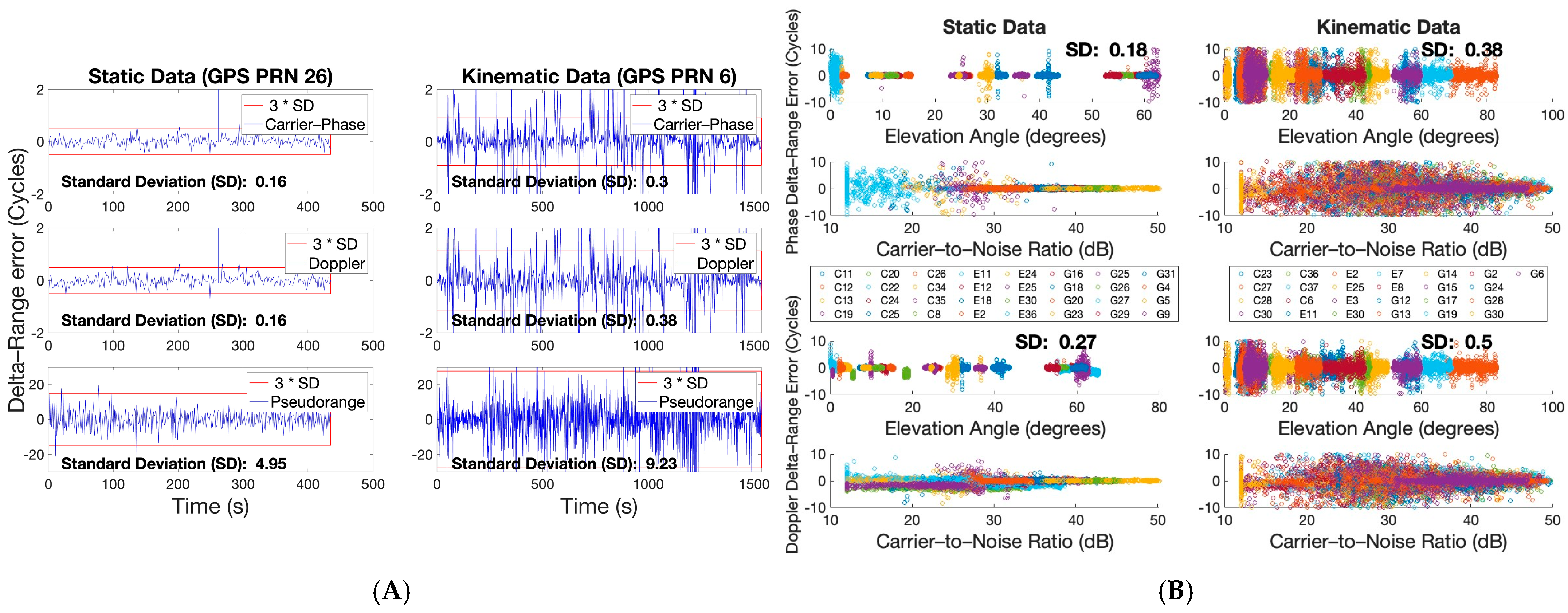
• CS Repair: The integer ambiguity resolution/fix is highly dependant on the variance of the TDCP measurement. Weighted variance mapping will produce large variance, in general, for TDCP measurements that do not necessarily have much noise associated with them, with reference to the static data plot in Figure 1B. Satellites at lower elevation angles or with lower $C/N_0$ are prone to losing phase lock frequently, but that does not necessarily deteriorate the precision of the phase measurements.

Therefore, the $R_{TDCP}$ is set to be the same for all the satellites. The choice of TDCP standard deviation/variance is crucial for CSDR and, following the analysis of TDCP error in Figure 1B, the SD is chosen as ~0.2 cycles or ~4 cm for both static and kinematic datasets. This choice stems from the fact that both datasets use smartphones equipped with the same GNSS chipset, BCM47755. Given that the TDCP SD for the static dataset was calculated as 0.18 cycles in Figure 1B, this value is deemed a reliable representation of chipset quality, justifying its uniform application across both datasets.

7. Experimental Results

The proposed method was applied to the two datasets. The CSs detected and repaired for both datasets are shown in

Table 1. Cycle Slip detection and repair rate.

Static Dataset				Kinematic Dataset
Inliers	CS detected		CS repaired	Inliers	CS detected		CS repaired
10,249	213		167	30,301	5420		2200
CS detection rate		CS repair rate		CS detection rate		CS repair rate
2.08%		78.40%		17.89%		40.60%

Note: TDCP standard deviation is chosen as ~0.2 cycle or ~4 cm for both datasets.

and Figure 3. Fewer CSs exist in the static data. The CS detection rate for static data is 2.08%, compared to 17.88% for kinematic data.

The leftmost two plots in Figure 3 show the TDCP errors labelled as inliers, detected as CSs, and selected for repair by the proposed method. In the right two plots in Figure 3 the red points (selected for repair) are shown corrected by the CS integer value. Figure 4 shows the corresponding histograms similarly labelled as inliers, CS detected, and CS repaired, from Figure 3. The TDCP errors after repair are clearly zero-mean Gaussian, similar to in the inliers histogram.

To demonstrate the working of the proposed CSDR method, results for certain epochs are presented in

Table 2. Summary of CSDR results for certain epochs for both static and kinematic data.

Static Dataset
Epoch	CS Detected	CS Repaired	Float CS Ambiguity	Fixed CS Ambiguity	Type of Repair	Success Rate LB	$\mathbf{FF}\text{-}\mathbf{RT}\text{-}\mathbf{Derived} \mathit{\mu }$	Ratio
17	G23, C24	G23, C24	[1.968, 5.93]	[2, 6]	FAR	91.94%	0.325	0.006
28	E25	E25	[1.343]	[1]	FAR	95.2%	0.401	0.274
97	G31, C25	C25	[−2.399, 2.951]	[3]	PAR	96.1%	0.486	0.003
327	C34	-	[−2.478]	-	-	96%	0.448	0.843
Kinematic Dataset
Epoch	CS Detected	CS Repaired	Float CS Ambiguity	Fixed CS Ambiguity	Type of Repair	Success Rate LB	FF-RT-Derived$\mathit{\mu }$	Ratio
42	G30, E2	G30, E2	[1.939, 3.034]	[2, 3]	FAR	87.77%	0.246	0.005
55	G6, G13, G14, G15, G17, G30, E7, E30, C6, C23, C27, C28, C36	G6, G13, G14, G15, G17, G30, E7, E30, C27, C28	[−3.35, 1.11, −1.24, 0.84, 0.96, −2.18, 28.25, 0.77, 6.58, −7.78, 0.82, 3.89, 2.01]	[−3, 1, −1, 1, 1, −2, 28, 1, 1, 4]	PAR	50.59%	0.55	0.54
120	G19, G30, E8, C6	G19, E8	[−0.795, −1.639, −31.989, 5.88]	[−1, −32]	PAR	89.58%	0.328	0.066
458	G13, E11, E30, C6, C36	G13, E11, E30, C36	[3.852, 14.95, 2.065, 5.641, 3.162]	[4, 15, 2, 3]	PAR	77.44%	0.246	0.077
1005	G14, G15, G28, E7, E8	G14, G15, G28, E7, E8	[1.765, −6.039, 5.016, 15.899, −2.119]	[2, −6, 5, 16, −2]	FAR	70.58%	0.216	0.126
Note: For PAR, float CS ambiguities which are not fixed to an integer still are adjusted due to other fixed ambiguities. For FF-RT, the fixed failure rate is taken as 1%.

. For the static data, usually no more than a couple of CSs occur at an epoch and therefore full ambiguity resolution (FAR) is possible for most of the detected CSs. This is not the case with kinematic data, for which as many as 13 CSs were detected at epoch 55, 10 of which could be fixed with a bootstrapping success rate lower bound (LB) of ~50%. The kinematic repair rate is lower (40.60%) compared to the static rate (78.40%), because it is more difficult to resolve a larger set of CS ambiguities. For the FF-RT-based integer validation test, a failure rate of 1% is chosen, which means that after the integer fix, a success rate LB of greater than 99% is required for the fix to be declared successful; otherwise a ratio test will be performed based on the adaptive threshold, $\mu$ [29]. For both the static and kinematic data, the requisite success rate LB of 99% is never achieved, leading to a ratio test at each epoch for validation.

The receiver velocity/delta-position estimated from the proposed CSDR filter will be compared against an identical KF, which only performs Doppler updates and does not integrate TDCP measurements.

Table 3. Velocity RMSE results.

	Static Data		Kinematic Data
Method/RMSE (mm/s)	Doppler-Only KF	Proposed CSDR Method	Doppler-Only KF	Proposed CSDR Method
East	33.90	6.51	62.26	33.75
North	44.82	44.80	99.92	71.40
Up	92.53	27.73	89.43	90.08
2D Error	56.20	45.27	117.73	78.98
3D Error	108.26	53.09	147.85	119.80

shows the velocity RMSE error in mm/s, for the proposed CSDR method and Doppler-only KF. It is evident that the proposed CSDR method results are more accurate.

8. Conclusions and Future Scope

A real-time single-frequency-based CSDR method based on a time-differenced model was proposed for Smartphone GNSS. CS detection and repair were shown to be heavily influenced by the assumed variance of TDCP measurements. The CS detection performance appears good, although a few false alarms exist for kinematic data. The kinematic data faces frequent CSs, making achieving reliable integer fix challenging, as the success rate decreases with the increasing number of CSs that need to be repaired. Even for static data, the computed success rate lower bound never satisfies the user-defined failure rate of 1%, and a ratio test based on FF-RT is always performed to validate the integer fix. Therefore, reliable CS detection is possible for single-frequency Smartphone GNSSs, but CS repair is hindered by the precision quality of the phase measurement. Future work will entail implementing the proposed CSDR method on L5 signals and the wide-lane phase measurements derived from dual-frequency signals.

References

1. Paziewski, J.; Fortunato, M.; Mazzoni, A.; Odolinski, R. An analysis of multi-GNSS observations tracked by recent Android smartphones and smartphone-only relative positioning results. Measurement 2021, 175, 109162. [Google Scholar] [CrossRef]
2. Goad, C.C. Precise positioning with the GPS. In Lecture Notes in Earth Sciences; Turner, S., Ed.; Springer: Berlin/Heidelberg, Germany, 1987; Volume 12, pp. 17–30. [Google Scholar] [CrossRef]
3. Blewitt, G. An automatic editing algorithm for GPS data. Geophys. Res. Lett. 1990, 17, 199–202. [Google Scholar] [CrossRef]
4. Bastos, L.; Landau, H. Fixing cycle slips in dual-frequency kinematic GPS-applications using Kalman filtering. Manuscripta Geod. 1988, 13, 249–256. [Google Scholar] [CrossRef]
5. Hofmann-Wellenhof, B.; Lichtenegger, H.; Collins, J. Global Positioning System: Theory and Practice; Springer: Berlin/Heidelberg, Germany, 1994. [Google Scholar]
6. Zuofa, Y.G.L. Cycle Slip Detection and Ambiguity Resolution Algorithms for Dual-Frequency GPS Data Processing. Mar. Geod. 1999, 22, 169–181. [Google Scholar] [CrossRef]
7. Bisnath, S.B. Efficient, automated cycle-slip correction of dual-frequency kinematic GPS data. In Proceedings of the 13th International Technical Meeting of the Satellite Division of The Institute of Navigation (ION GPS 2000), Salt Lake City, UT, USA, 19–22 September 2000; pp. 145–154. [Google Scholar]
8. Fath-Allah, T.F. A new approach for cycle slips repairing using GPS single frequency data. World Appl. Sci. J. 2010, 8, 315–325. [Google Scholar]
9. Liu, Z. A new automated cycle slip detection and repair method for a single dual-frequency GPS receiver. J. Geod. 2011, 85, 171–183. [Google Scholar] [CrossRef]
10. Kim, D.; Langley, R.B. Instantaneous Real-Time Cycle-Slip Correction for Quality Control of GPS Carrier-Phase Measurements. Navigation 2002, 49, 205–222. [Google Scholar] [CrossRef]
11. Ren, Z.; Li, L.; Zhong, J.; Zhao, M. Instantaneous Cycle-Slip Detection and Repair of GPSData Based on Doppler Measurement. Int. J. Inf. Electron. Eng. 2012, 2, 96. [Google Scholar] [CrossRef]
12. Zhao, J.; Hernández-Pajares, M.; Li, Z.; Wang, L.; Yuan, H. High-rate Doppler-aided cycle slip detection and repair method for low-cost single-frequency receivers. Gps Solut. 2020, 24, 1–13. [Google Scholar] [CrossRef]
13. de Lacy, M.C.; Reguzzoni, M.; Sansò, F.; Venuti, G. The Bayesian detection of discontinuities in a polynomial regression and its application to the cycle-slip problem. J. Geod. 2008, 82, 527–542. [Google Scholar] [CrossRef]
14. Zangeneh-Nejad, F.; Amiri-Simkooei, A.R.; Sharifi, M.A.; Asgari, J. Cycle slip detection and repair of undifferenced single-frequency GPS carrier phase observations. GPS Solut. 2017, 21, 1593–1603. [Google Scholar] [CrossRef]
15. Leick, A. GPS Satellite Surveying, 2nd ed.; Wiley-Interscience: New York, NY, USA, 1995. [Google Scholar]
16. Teunissen, P. Quality Control and GPS. In GPS for Geodesy; Springer: Berlin/Heidelberg, Germany, 1998. [Google Scholar] [CrossRef]
17. Kubo, Y.; Sone, K.; Sugimoto, S. Cycle slip detection and correction for kinematic GPS based on statistical tests of innovation processes. In Proceedings of the 17th International Technical Meeting of the Satellite Division of The Institute of Navigation (ION GNSS 2004), Long Beach, CA, USA, 21–24 September 2004; pp. 1438–1447. [Google Scholar]
18. Lin, S.-G.; Yu, F.-C. Cycle slips detection algorithm for low cost single frequency GPS RTK positioning. Surv. Rev. 2013, 45, 206–214. [Google Scholar] [CrossRef]
19. Banville, S.; Langley, R.B. Cycle-slip correction for single-frequency PPP. In Proceedings of the 25th International Technical Meeting of the Satellite Division of The Institute of Navigation (ION GNSS 2012), Nashville, TN, USA, 17–21 September 2012; pp. 3753–3761. [Google Scholar]
20. Li, P.; Jiang, X.; Zhang, X.; Ge, M.; Schuh, H. Kalman-filter-based undifferenced cycle slip estimation in real-time precise point positioning. GPS Solut. 2019, 23, 1–13. [Google Scholar] [CrossRef]
21. Kirkko-Jaakkola, M.; Traugott, J.; Odijk, D.; Collin, J.; Sachs, G.; Holzapfel, F. A RAIM approach to GNSS outlier and cycle slip detection using L1 carrier phase time-differences. In Proceedings of the 2009 IEEE Workshop on Signal Processing Systems, Tampere, Finland, 7–9 October 2009; pp. 273–278. [Google Scholar]
22. Li, T.; Melachroinos, S. An enhanced cycle slip repair algorithm for real-time multi-GNSS, multi-frequency data processing. GPS Solut. 2019, 23, 1–11. [Google Scholar] [CrossRef]
23. Carcanague, S. Real-time geometry-based cycle slip resolution technique for single-frequency PPP and RTK. In Proceedings of the 25th International Technical Meeting of The Satellite Division of the Institute of Navigation (ION GNSS 2012), Nashville, TN, USA, 17–21 September 2012; pp. 1136–1148. [Google Scholar]
24. Banville, S.; Langley, R.B. Instantaneous Cycle-Slip Correction for Real-Time PPP Applications. Navigation 2010, 57, 325–334. [Google Scholar] [CrossRef]
25. Li, B.; Liu, T.; Nie, L.; Qin, Y. Single-frequency GNSS cycle slip estimation with positional polynomial constraint. J. Geod. 2019, 93, 1781–1803. [Google Scholar] [CrossRef]
26. Teunissen, P.J.G. Carrier Phase Integer Ambiguity Resolution. In Springer Handbook of Global Navigation Satellite Systems; Teunissen, P.J.G., Montenbruck, O., Eds.; Springer International Publishing: Cham, Switzerlands, 2017; pp. 661–685. [Google Scholar] [CrossRef]
27. SmartphonesCampaign2021.docx. Google Docs. Available online: https://docs.google.com/document/d/1XlQ9uarBDJEGsWOOHjYiPXkg4W3AH9qc/edit?usp=embed_facebook (accessed on 9 May 2024).
28. Fu, G.; Khider, M.; van Diggelen, F. Google Smartphone Decimeter Challenge. May 2021. Available online: https://www.kaggle.com/c/google-smartphone-decimeter-challenge/data (accessed on 9 May 2024).
29. Verhagen, S.; Li, B. LAMBDA Software Package: Matlab Implementation; Version 3.0; Delft University of Technology and Curtin University: Perth, Australia, 2012. [Google Scholar]
30. Tay, S.; Marais, J. Weighting models for GPS Pseudorange observations for land transportation in urban canyons. In Proceedings of the 6th European Workshop on GNSS Signals and Signal Processing, Munich, Germany, 5–6 December 2013. [Google Scholar]
Figure 1. (A) Delta-range error (in blue) for a single satellite in cycles with 3 times the standard deviation (in red). (B) Carrier phase and Doppler derived delta-range error in cycles for all GPS L1 + GALE1+ BDS B1I signals, with the overall standard deviation indicated in bold.
Engproc 88 00010 g001
Figure 2. Test quantity for different GF-CSD combinations. The L1 signal is used for single-frequency-based GF-CSD combinations, namely PMC and phase-prediction. 3 times the sample standard deviation is shown in red.
Engproc 88 00010 g002
Figure 3. Proposed CSDR results. The right two plot columns show TDCP error adjusted by the repaired integer CS ambiguities.
Engproc 88 00010 g003
Figure 4. Corresponding histograms for Figure 3.
Engproc 88 00010 g004