Comparing FCNN and LSTM Architectures for Magnetic Field Prediction Using an All-Optical NV Diamond Setup ^†

Abstract

This paper investigates the prediction of magnetic fields using an all-optical NV diamond sensing setup combined with neural network models. In contrast to previous work, the focus is placed on the generalization capability of the models across independent measurement data sets affected by drift. Three architectures are evaluated: two fully connected neural networks (FCNNs) and one long short-term memory (LSTM) network. The LSTM network achieves improved prediction accuracy compared to the FCNNs due to the use of sequences instead of individual values. The inclusion of temperature as an additional input feature further enhances performance. However, significant discrepancies between measurement data sets, caused by drift, prevent reliable generalization across data sets for all models. These findings indicate that improving hardware stability is essential for achieving robust real-world performance of data-driven NV-based sensing systems.

1. Introduction

Quantum sensors based on nitrogen-vacancy (NV) centers in diamonds have emerged as a promising sensing technology due to their atomic-scale size, room-temperature operation, and sensitivity to a wide range of physical quantities [1,2,3]. NV centers are point defects in the diamond lattice whose spin-dependent fluorescence properties enable the detection of magnetic fields [4,5,6], electric fields [7,8], temperature [9,10], pressure [11], or strain [12]. This property makes them a highly flexible sensing platform with a wide range of applications.

The sensing of magnetic fields through the use of NV centers can be achieved through different approaches. Optically detected magnetic resonance (ODMR) is a well-established technique in which microwave radiation drives the spin transitions of the NV center. The resulting fluorescence changes depend on the spin state of the NV center and are used to detect shifts in the resonance frequency induced by an external magnetic field. This approach enables sensitivities in the pico-Tesla range and below [13,14]. An alternative approach is all-optical sensing, which eliminates the need for microwave components by directly measuring fluorescence intensity changes resulting from spin mixing within the NV center. While this approach yields lower sensitivity compared to ODMR, the reduced hardware requirements make it a practical solution for real-world deployment [15,16,17].

In previous work [18,19], a fully connected neural network (FCNN) was employed to predict magnetic field values from fluorescence lifetime measurements conducted in the frequency domain using an all-optical sensing approach. However, measurement drift was not accounted for in the aforementioned work. This drift originates from various factors, including ambient temperature variations and hardware instabilities. Such factors lead to systematic differences between measurements that are difficult to capture with a model trained on a single data set. Since drift varies between measurements, a model trained on one data set cannot readily be applied to another without a significant loss in prediction accuracy. Such generalization is essential for practical real-world applications, where retraining or collecting new labeled data for each new measurement is not feasible. However, the ability of neural network models to generalize across independently acquired data sets affected by measurement drift has not yet been systematically investigated.

To address this limitation, two FCNN architectures and one long short-term memory (LSTM) architecture are compared regarding their ability to handle temporal dependencies and data set variations. Furthermore, the impact of temperature as an additional input feature is analyzed. The use of simulated data and data augmentation during training is additionally evaluated. The results reveal that the LSTM model improves prediction accuracy. However, measurement drift emerges as a key challenge for cross-data set generalization.

2. Materials and Methods

2.1. Experimental Setup and Measured Data Sets

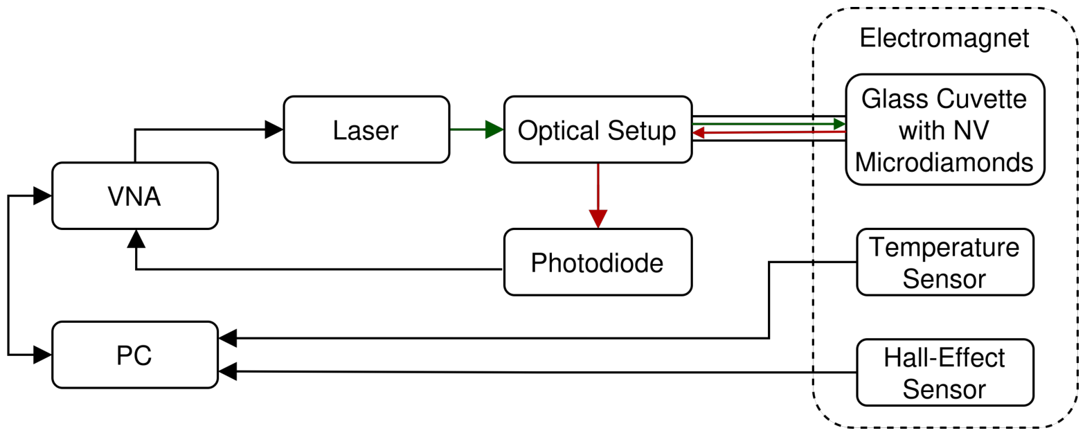
The present work utilizes an existing fluorescence lifetime measurement setup in the frequency domain, which was extended by an additional temperature measurement. The block diagram of the experimental setup is shown in Figure 1. A more detailed description of the setup can be found in [19].

A glass cuvette containing NV-rich microdiamonds, along with the end facet of a fiber, is placed within an electromagnet, which generates a magnetic field in the range of 0 to 18 mT. The magnetic field is measured for data-labeling purposes using a Hall-effect sensor, which is positioned adjacent to the glass cuvette. The temperature within the electromagnet is recorded as an additional measurement quantity. The NV diamonds are excited by green laser light from a laser diode. The frequency at which the laser diode is switched ranges from 1 to 100 MHz, with 401 equidistant steps. The frequency sweep is conducted with a vector network analyzer (VNA). The green laser light is coupled into the fiber via an optical setup. The NV diamonds emit a red fluorescence that is led to the photodiode via the same fiber and optical setup. The amplitude and phase of the photodiode signal are recorded at the VNA.

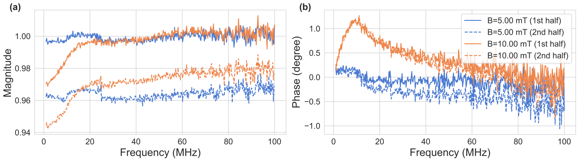
The measurement process encompasses five frequency sweeps, from which the mean values are calculated. For every applied magnetic field, one value for amplitude and one value for phase are recorded at each frequency. This results in a total of 401 values for amplitude and phase. Figure 2 shows the magnitude and phase for two different magnetic field values from MEAS_1, with one sample taken from the first half of the data set and one from the second half. A noticeable difference between the two halves can be observed, particularly in magnitude, which is attributed to the measurement drift. Additionally, the differences in magnitude and phase among various magnetic field values are most apparent in the lower half of the frequency range.

A total of three measurement series, each comprising 20,000 measurements, were carried out. Each measurement series is considered a distinct data set, designated as MEAS_1, MEAS_2, and MEAS_3 in the following. The sequence of the applied magnetic fields is arbitrary but uniform across all three data sets. Furthermore, every 20th measurement is conducted under a magnetic field of $B=0 \mathrm{mT}$. These zero-field measurements allow for a more detailed observation of the drift over time. Moreover, the results from [19] have shown that the FCNN used in that work achieved better performance when the additional measurements at $B=0 \mathrm{mT}$ were included.

2.2. Simulation-Based Data Set

The simulation-based data set contains simulations of the fluorescence lifetime in the frequency domain for 1000 different magnetic fields. The range of the magnetic fields is equivalent to that of the measurements, with values ranging from 0 to 18 mT. Notably, the data points are not uniformly distributed, as 500 values are concentrated in the range from 0 to 8 mT, whereas the remaining 500 values extend over the wider range from 8 to 18 mT. This split was selected because the largest deviations in the prediction of the magnetic field occurred in the previous work for fields below 8 mT [18,19]. The frequency sweep is limited to the range from 1 to 50 MHz, resulting in 201 values each for magnitude and phase. This reduced frequency range is chosen because the largest differences in magnitude and phase between different magnetic field values occur in the lower-frequency region, as shown in Figure 2. The simulation data set was duplicated 20 times to match the size of the measured training data, ensuring a balanced representation of both data sources during training.

2.3. Neural Network Architectures

In this work, three neural network architectures are examined: two FCNNs and one LSTM network. For all three models, the input consists of 201 magnitude and 201 phase values, concatenated to form a feature vector of length 402. Moreover, temperature can be utilized as an additional input feature. In such cases, the feature vector length increases to 403. The output target is the predicted magnetic field value, and the mean absolute error (MAE) is used as the loss function for all models. All input features are scaled using a MinMaxScaler, which was fitted exclusively on the training data to prevent data leakage.

The first FCNN model, referred to as FCNN-Base, follows the architecture established and validated in previous work [19]. This model consists of the input layer; three hidden layers with 50, 20, and 5 nodes, respectively; and a single output node. The second FCNN model, referred to as FCNN-Ext, extends this architecture with an additional hidden layer containing 64 nodes that is inserted directly after the input layer. This extension was introduced to determine whether using an additional layer, and thus a larger model, can yield better results than FCNN-Base. In both FCNNs, all hidden layers utilize a ReLU activation function, while the output layer does not employ any activation function.

The LSTM model under consideration consists of a single bidirectional LSTM layer with a hidden size of 64, which doubles to an output size of 128 due to the concatenation of forward and backward pass outputs. This output is subsequently passed through three fully connected layers with 50, 20, and 5 nodes, respectively, each employing a ReLU activation function, followed by a single output node. The fully connected layers are kept identical in size to the hidden layers of the FCNNs to ensure comparability across the architectures.

2.4. Training and Data Configuration

All models are trained using the Adam optimizer with a learning rate of $2.02·{10}^{-4}$, which was determined via hyperparameter tuning. Both FCNNs utilize a batch size of 16, whereas the LSTM model uses a batch size of 32. In order to prevent overfitting, early stopping is applied to all models with a patience of 50 epochs and a minimum MAE improvement threshold of $1·{10}^{-6}$. In addition, a learning rate scheduler is implemented for all models. The scheduler reduces the learning rate by a factor of 0.5 once the loss function reaches a plateau, with a patience of 20 epochs.

From the measured data, only the first 201 frequency points are used to match the frequency range of the simulation data. One of the three measured data sets is used for training and validation, while the remaining two are held out for testing. For the LSTM model, the input data is organized into sequences, each consisting of 20 consecutive measurements, where the target value corresponds to the last element of each sequence. The sequence length was determined through hyperparameter tuning. Furthermore, since every 20th measurement is at $B=0 \mathrm{mT}$, each sequence of length 20 contains a zero-field measurement. The data is not shuffled before sequencing in order to preserve the temporal order of the measurements.

From MEAS_1, which is selected for training, 60% are used for training and 20% are used for validation. The remaining two data sets, MEAS_2 and MEAS_3, are kept entirely separate and serve as independent test sets. Two splitting strategies are considered. In the first variant, referred to as the temporal split, the first 60% of the data set is used for training and the final 20% is used for validation, thereby preserving the temporal order of the data set. In the second variant, the data set is shuffled prior to splitting so that random subsets of 60% and 20% are assigned to training and validation, respectively. This variant is referred to as the random split.

To assess the influence of temperature, the models are evaluated both with and without temperature as an additional input feature. Building on the findings regarding the use of temperature, four training data configurations are examined. These comprise (1) using only the measured training data, referred to as RAW; (2) the RAW configuration with additional online data augmentation, referred to as RAW + AUG; (3) the measured training data combined with the full simulation data set, referred to as SIM; and (4) the SIM configuration with additional online data augmentation, referred to as SIM + AUG. The purpose of online data augmentation is to emulate the effect of measurement drift. By introducing variation, a more diverse training set that covers a broader range of conditions is created. This encourages better generalization, as the model is no longer trained exclusively on exact measured values. The online data augmentation method works as follows: During training, each sample has a 50% chance of being augmented in each epoch. When augmentation is applied, the magnitude and phase values are each multiplied by a random scaling factor, drawn independently from a uniform distribution. For magnitude, the scaling factor lies in the range $[0.98,1.01]$, while for phase it lies in the range $[0.99,1.01]$. Since these factors are resampled in every epoch, the same sample may be scaled differently across epochs. The wider scaling range for magnitude reflects its higher sensitivity to measurement drift compared to that of the phase, as shown in Figure 2. The scaling ranges were selected to approximate the relative magnitude and phase variations observed in the measurement data.

3. Results

For the evaluation of the trained models, the MAE and the root mean square error (RMSE) are used. First, the three models (FCNN-Base, FCNN-Ext, and LSTM) are compared regarding the input feature vector. The results are presented in

Table 1. MAE and RMSE (both in mT) for the models FCNN-Base, FCNN-Ext, and LSTM tested on the data sets MEAS_2 and MEAS_3. All models were trained on the MEAS_1 data set. Results are reported for two configurations: without (no T) and with (with T) temperature as an additional input feature. Each configuration is evaluated using both a temporal split and a random split of MEAS_1. The best values per column are indicated in bold.

		Temporal Split				Random Split
		MEAS_2		MEAS_3		MEAS_2		MEAS_3
		MAE	RMSE	MAE	RMSE	MAE	RMSE	MAE	RMSE
FCNN-Base	no T	0.741	0.941	0.707	0.964	0.520	0.688	0.699	0.902
	with T	0.704	0.904	0.671	0.853	0.491	0.690	0.614	0.795
FCNN-Ext	no T	0.703	0.968	0.719	1.040	0.461	0.631	0.634	0.791
	with T	0.770	1.008	0.700	0.937	0.468	0.679	0.693	0.866
LSTM	no T	0.555	0.797	0.691	0.813	0.413	0.585	0.842	1.053
	with T	0.488	0.646	0.652	0.794	0.325	0.467	0.848	1.001

. The rows labeled no T correspond to using only magnitude and phase as input features, while the row with T corresponds to including temperature as an additional input feature. Both the temporal split and the random split are considered in this comparison.

The influence of including temperature as an input feature is examined first. For FCNN-Base, the inclusion of temperature consistently leads to better results across all configurations. The LSTM model shows a similar trend, with the only exception being a marginally lower MAE for the configuration without temperature when using the random split and the test set MEAS_3. For the FCNN-Ext, however, including temperature is only beneficial for the temporal split evaluated on MEAS_3. In all other cases, the FCNN-Ext model performs better without temperature as an input feature.

With respect to the splitting strategies, both FCNNs consistently achieve better results with the random split. For LSTM, the preferred split depends on the test set. The temporal split yields better performance on MEAS_2, while the random split is more favorable for MEAS_3.

A further observation is that the results often differ considerably between the two test sets. With the random split, all models perform better on MEAS_2 than on MEAS_3. The same holds for the LSTM model with the temporal split. For both FCNNs under the temporal split, the results are more mixed, and the differences between the two test sets are the smallest.

Comparing FCNN-Base and FCNN-Ext, neither model shows a clear advantage over the other. Among all three models, the LSTM model consistently outperforms both FCNNs. For MEAS_2, LSTM achieves the best results in terms of both MAE and RMSE, regardless of the split strategy. For MEAS_3, the LSTM model performs best with the temporal split. Only for MEAS_3 with the random split do both FCNNs outperform the LSTM model. The improved performance of the LSTM model may be due to its capacity to leverage the sequential nature of the data, potentially capturing temporal drift patterns, the fixed measurement structure, or a combination of both. In contrast, FCNN models treat each sample independently and therefore cannot exploit such sequential information.

In the next step, the influence of simulation data and online data augmentation on the training process is investigated. In all configurations, magnitude and phase together with temperature are used as input features. Both the temporal split and the random split are considered. Since the LSTM model outperformed the FCNN-Base and FCNN-Ext models in the previous analysis, only the LSTM model is evaluated in this comparison. The results are shown in

Table 2. MAE and RMSE (both in mT) for the model LSTM tested on the data sets MEAS_2 and MEAS_3. The model was trained on the MEAS_1 data set. Results are reported for the training with the training data set (RAW), the training data together with online data augmentation (RAW + AUG), the training data with the simulation data (SIM), and the training data with the simulation data and online data augmentation (SIM + AUG). Each configuration is evaluated using both a temporal split and a random split of MEAS_1. The best values per column are indicated in bold.

	Temporal Split				Random Split
	MEAS_2		MEAS_3		MEAS_2		MEAS_3
	MAE	RMSE	MAE	RMSE	MAE	RMSE	MAE	RMSE
RAW	0.488	0.646	0.652	0.794	0.325	0.467	0.848	1.001
RAW + AUG	0.477	0.695	0.751	0.932	0.423	0.640	0.765	0.884
SIM	0.527	0.711	0.665	0.942	0.340	0.485	0.963	1.146
SIM + AUG	0.428	0.583	0.976	1.232	0.375	0.520	1.019	1.218

.

The best results for each test set are achieved using only the measured training data (RAW), in particular with the random split for MEAS_2 and with the temporal split for MEAS_3. Adding simulation data to the training set does not improve the results. Online data augmentation, however, can provide a benefit in certain cases. This benefit is observed for the temporal split with the MEAS_2 test set, where the combination of simulation data, measured training data, and online data augmentation (SIM + AUG) yields the best result. Likewise, for the random split with the MEAS_3 test set, the measured training data with online data augmentation but without simulation data (RAW + AUG) achieves the best performance.

Across all training data configurations, the results on the MEAS_2 test set are consistently better than those on MEAS_3. This trend is in line with the observations from Table 1, confirming that this trend persists regardless of the training data configuration. The significant performance differences between MEAS_2 and MEAS_3 indicate that the models are not only sensitive to noise but also to systematic data set-specific variations.

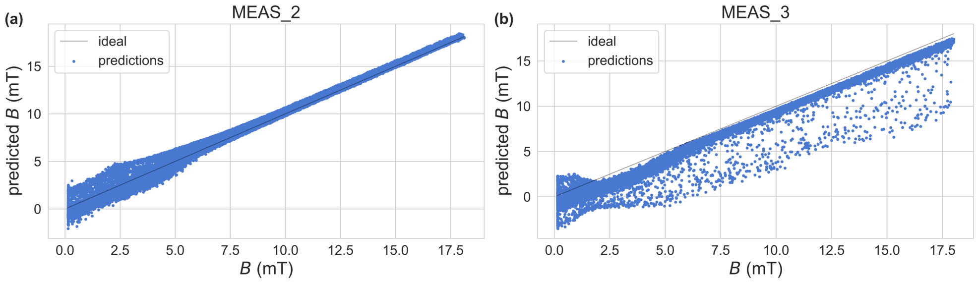
To further illustrate these differences, Figure 3 visualizes the prediction behavior of the LSTM model trained on MEAS_1 with the random split, without online data augmentation or simulation data (RAW). The predicted magnetic field values are plotted against the reference values for both test sets (MEAS_2 and MEAS_3). A notable difference in the prediction characteristics can be observed between the two test sets. For MEAS_2, the model tends to overestimate the magnetic field, whereas for MEAS_3, the predicted values mostly fall below the ideal prediction. Additionally, MEAS_3 exhibits a large number of outliers. For MEAS_2, the largest deviations occur in the lower-magnetic-field range up to about $7.5$ mT.

4. Conclusions

In this work, three neural network architectures, two FCNNs and one LSTM, were evaluated for the prediction of the magnetic field from frequency-domain fluorescence lifetime measurement data across various training data configurations. One measured data set was used entirely for training and validation, while two additional measured data sets were reserved for testing.

Among the investigated input configurations, including temperature as an additional input feature together with magnitude and phase proved to be clearly beneficial. This simple extension of the input vector improved the results for the models FCNN-Base and LSTM across both test sets.

Increasing the model size from FCNN-Base to FCNN-Ext did not consistently improve performance. This finding suggests that model capacity is not the limiting factor. Instead, the systematic variations introduced by measurement drift cannot be resolved by additional layers alone. The LSTM model, however, outperformed both FCNN variants. Its use of sequences containing temporally consecutive measurements, within which the drift characteristics remain similar, led to better predictions compared to processing individual samples independently. However, it cannot be ruled out that the LSTM model exploits the identical ordering of magnetic field values across all three data sets. To investigate this possibility, additional data sets featuring different magnetic field sequences would need to be used for training and validation. Simply shuffling the data before creating the sequences is not a viable alternative because this would disrupt the temporal continuity that the model relies on to capture drift behavior within each sequence.

Despite this improvement, the considerable differences in prediction performance between the two test sets, particularly for the LSTM model, reveal a fundamental limitation of the current experimental setup. Measurement drift introduces data set-specific characteristics that cannot be compensated by the considered machine learning models alone. Consequently, improving hardware stability is a prerequisite for achieving robust generalization in practical applications. Additionally, a rotating training scheme, in which each data set alternates between training and test data, could help ensure more robust generalization.

Beyond architectural choices, extending the training data with simulation data to improve generalization did not lead to better results. Online data augmentation was introduced to emulate measurement drift and to create a more diverse training set no longer based on a single measurement alone. However, it did not provide a clear and consistent advantage either. The limited benefit of simulation data suggests that the simulated signals do not sufficiently capture the complexity of real measurement conditions, particularly with respect to drift and other environmental influences.

Regarding the choice of data split for training the LSTM model, no general recommendation can be made in favor of either the temporal split or the random split, as the preferred strategy depends on the training data configuration and the test set under consideration.

Future work should focus on reducing measurement drift through hardware modifications. Furthermore, the previously mentioned rotating training scheme should be investigated to better assess and improve the generalization capability of the models. To further validate the LSTM results, additional data sets with varying magnetic field sequences should be acquired to rule out the possibility that the model exploits the identical ordering across the current data sets. Additionally, domain adaptation techniques could be explored to improve cross-data set generalization without requiring complete retraining for each new measurement.

References

- Tetienne, J.P.; Rondin, L.; Spinicelli, P.; Chipaux, M.; Debuisschert, T.; Roch, J.F.; Jacques, V. Magnetic-Field-Dependent Photodynamics of Single NV Defects in Diamond: An Application to Qualitative All-Optical Magnetic Imaging. New J. Phys. 2012, 14, 103033. [Google Scholar] [CrossRef] [Scilit]
- Doherty, M.W.; Manson, N.B.; Delaney, P.; Jelezko, F.; Wrachtrup, J.; Hollenberg, L.C. The nitrogen-vacancy colour centre in diamond. Phys. Rep. 2013, 528, 1–45. [Google Scholar] [CrossRef] [Scilit]
- Rondin, L.; Tetienne, J.P.; Hingant, T.; Roch, J.F.; Maletinsky, P.; Jacques, V. Magnetometry with Nitrogen-Vacancy Defects in Diamond. Rep. Prog. Phys. 2014, 77, 056503. [Google Scholar] [CrossRef] [Scilit]
- Chatzidrosos, G.; Rebeirro, J.S.; Zheng, H.; Omar, M.; Brenneis, A.; Stürner, F.M.; Fuchs, T.; Buck, T.; Rölver, R.; Schneemann, T.; et al. Fiberized Diamond-Based Vector Magnetometers. Front. Photonics 2021, 2, 732748. [Google Scholar] [CrossRef] [Scilit]
- Homrighausen, J.; Hoffmann, F.; Pogorzelski, J.; Glösekötter, P.; Gregor, M. Microscale fiber-integrated vector magnetometer with on-tip field biasing using N-V ensembles in diamond microcrystals. Phys. Rev. Appl. 2024, 22, 034029. [Google Scholar] [CrossRef] [Scilit]
- Dhungel, O.; Mrózek, M.; Lenz, T.; Ivády, V.; Gali, A.; Wickenbrock, A.; Budker, D.; Gawlik, W.; Wojciechowski, A.M. Near-zero-field microwave-free magnetometry with nitrogen-vacancy centers in nanodiamonds. Opt. Express 2024, 32, 21936–21945. [Google Scholar] [CrossRef] [Scilit]
- Dolde, F.; Fedder, H.; Doherty, M.W.; Nöbauer, T.; Rempp, F.; Balasubramanian, G.; Wolf, T.; Reinhard, F.; Hollenberg, L.C.L.; Jelezko, F.; et al. Electric-field sensing using single diamond spins. Nat. Phys. 2011, 7, 459–463. [Google Scholar] [CrossRef] [Scilit]
- Styles, R.; Han, M.; Goris, T.; Partridge, J.G.; Johnson, B.C.; Rosal, B.D.; Abraham, A.N.; Ebendorff-Heidepriem, H.; Gibson, B.C.; Dontschuk, N.; et al. All-Optical Electric Field Sensing with Nanodiamond-Doped Polymer Thin Films. Adv. Funct. Mater. 2025, 35, e12068. [Google Scholar] [CrossRef] [Scilit]
- Fujiwara, M.; Shikano, Y. Diamond quantum thermometry: From foundations to applications. Nanotechnology 2021, 32, 482002. [Google Scholar] [CrossRef] [Scilit]
- Acosta, V.M.; Bauch, E.; Ledbetter, M.P.; Waxman, A.; Bouchard, L.S.; Budker, D. Temperature Dependence of the Nitrogen-Vacancy Magnetic Resonance in Diamond. Phys. Rev. Lett. 2010, 104, 070801. [Google Scholar] [CrossRef] [Scilit]
- Doherty, M.W.; Struzhkin, V.V.; Simpson, D.A.; McGuinness, L.P.; Meng, Y.; Stacey, A.; Karle, T.J.; Hemley, R.J.; Manson, N.B.; Hollenberg, L.C.L.; et al. Electronic Properties and Metrology Applications of the Diamond NV− Center under Pressure. Phys. Rev. Lett. 2014, 112, 047601. [Google Scholar] [CrossRef] [Scilit]
- Trusheim, M.E.; Englund, D. Wide-field strain imaging with preferentially aligned nitrogen-vacancy centers in polycrystalline diamond. New J. Phys. 2016, 18, 123023. [Google Scholar] [CrossRef] [Scilit]
- Stürner, F.M.; Brenneis, A.; Buck, T.; Kassel, J.; Rölver, R.; Fuchs, T.; Savitsky, A.; Suter, D.; Grimmel, J.; Hengesbach, S.; et al. Integrated and Portable Magnetometer Based on Nitrogen-Vacancy Ensembles in Diamond. Adv. Quantum Technol. 2021, 4, 2000111. [Google Scholar] [CrossRef] [Scilit]
- Xie, Y.; Yu, H.; Zhu, Y.; Qin, X.; Rong, X.; Duan, C.K.; Du, J. A Hybrid Magnetometer towards Femtotesla Sensitivity under Ambient Conditions. Sci. Bull. 2021, 66, 127–132. [Google Scholar] [CrossRef] [Scilit]
- Staacke, R.; John, R.; Wunderlich, R.; Horsthemke, L.; Knolle, W.; Laube, C.; Glösekötter, P.; Burchard, B.; Abel, B.; Meijer, J. Isotropic Scalar Quantum Sensing of Magnetic Fields for Industrial Application. Adv. Quantum Technol. 2020, 3, 2000037. [Google Scholar] [CrossRef] [Scilit]
- Bähr, M.; Jahn, M.; Heinze, C.; Neckermann, K.; Meijer, J.; Ortlepp, T. Compact All-Optical Quantum Sensor Device Based on Nitrogen Vacancy Centers in Diamond. Phys. Status Solidi A 2023, 220, 2200338. [Google Scholar] [CrossRef] [Scilit]
- Paone, D.; Pinto, D.; Kim, G.; Feng, L.; Kim, M.J.; Stöhr, R.; Singha, A.; Kaiser, S.; Logvenov, G.; Keimer, B.; et al. All-optical and microwave-free detection of Meissner screening using nitrogen-vacancy centers in diamond. J. Appl. Phys. 2021, 129, 024306. [Google Scholar] [CrossRef] [Scilit]
- Horsthemke, L.; Pogorzelski, J.; Stiegekötter, D.; Hoffmann, F.; Bülter, A.S.; Trinschek, S.; Gregor, M.; Glösekötter, P. Towards Resolving the Ambiguity in Low-Field, All-Optical Magnetic Field Sensing with High NV-Density Diamonds. Eng. Proc. 2024, 68, 8. [Google Scholar] [CrossRef] [Scilit]
- Bülter, A.S.; Horsthemke, L.; Ávila Jiménez, J.L.; Hoffmann, F.; Rodriguez-Lozano, F.J.; Kirschke, S.; Sanders, T.; Gregor, M.; Glösekötter, P. Computational Approaches for Resolving the Low-Field Ambiguity in All-Optical Magnetic Field Sensing with NV Centers. In Proceedings of the Lecture Notes in Computer Science; Rojas, I., Joya, G., Catala, A., Eds.; Springer Nature: Cham, Switzerland, 2025; pp. 478–489. [Google Scholar] [CrossRef] [Scilit]