Comparison of Machine Learning Classifiers with PSO-Based Optimization and Correlation Feature Selection for Heart Disease Detection ^†

Abstract

Heart disease remains the leading cause of global mortality; therefore, rapid and accurate early detection is essential. This study proposes a hybrid machine learning framework integrating Correlation-Based Feature Selection (CFS) and Particle Swarm Optimization (PSO) to improve classification performance. The dataset was obtained from the Zenodo repository, which provides a compiled version of the UCI Heart Disease dataset consisting of 1025 instances with 14 clinical attributes. Five algorithms, Naive Bayes, Logistic Regression, K-Nearest Neighbors, Support Vector Machine, and Random Forest, were evaluated using 10-fold cross-validation. Results show that PSO improves classification performance, achieving accuracies between 82.81% and 84.48%, demonstrating the potential of the proposed framework for supporting early heart disease detection.

1. Introduction

Heart disease is a condition in which cardiac function is impaired due to abnormalities in blood vessels, heart rhythm, valves, or congenital defects, which can affect the heart’s ability to pump blood throughout the body [1]. Based on research conducted by the Indonesian Ministry of Health using population it was recorded that 1.5% of the population in Indonesia were diagnosed with heart disease [2]. Meanwhile, data from the World Health Organization (WHO) in 2022 estimated that approximately 19.8 million people died due to cardiovascular diseases, including heart disease, representing about 32% of all global deaths [3]. This problem becomes more critical because early detection is often overlooked, while the diagnostic process requires relatively high costs, as it must be conducted directly by medical specialists and supported by laboratory examinations [4]. To accelerate and improve the accuracy of the heart disease diagnosis process, machine learning (ML) models can be utilized [5].

Machine learning (ML) models operate by identifying characteristic patterns in data through method selection, followed by the adjustment of initial parameters such as the number of layers and learning rate via repeated evaluations until optimal classification and prediction accuracy is achieved [6]. Several studies have utilized machine learning-based classification techniques for heart disease diagnosis [7].

Classification works by identifying patterns and assigning objects to specific target class categories based on the similarity of their characteristics [8]. The selection of classification algorithms in relation to the quality of the features used is an important factor that affects machine learning model performance; therefore, the use of irrelevant features or those with weak relationships to the target class can reduce accuracy and increase model complexity. Consequently, the application of Correlation Feature Selection is required to identify and eliminate irrelevant attributes based on the degree of association between features and the target class in the heart disease diagnosis process [9,10].

Several studies on heart disease detection have been conducted using various machine learning methods, reporting accuracies of 84% for Naive Bayes, 84% for Logistic Regression, 81% for Random Forest, 81% for Support Vector Machine (SVM), 74% for Decision Tree, 73% for k-Nearest Neighbors (KNN), and 71% for Adaptive Boosting [11]. Other studies have reported accuracies of 94% for KNN, 93% for Decision Tree, 86% for Logistic Regression, and 85% for SVM [12,13]. A study on coronary heart disease using Logistic Regression obtained an accuracy of 82% [14]. Another study reported a significant decrease in accuracy, where the KNN model achieved only 64% [15]. In cardiovascular research related to heart disease, the Logistic Regression algorithm had an accuracy of 73% and Random Forest had an accuracy of 71% [16]. Another difference was that the accuracy results were 79% for the KNN algorithm and 79% for Naive Bayes, but Logistic Regression was only 76% [17]. Meanwhile, a more significant decrease occurred in the Support Vector Machine (SVM) algorithm, which had a much lower accuracy of 54.43% [18].

Several optimization approaches can be employed to improve accuracy, including the Whale Optimization Algorithm (WOA), Bat Algorithm (BA), Firefly Algorithm (FA), Ant Colony Optimization (ACO), Genetic Algorithm (GA), Dragonfly Algorithm (DA), Gray Wolf Optimizer (GWO), Cuckoo Search (CS), Artificial Bee Colony (ABC), and Particle Swarm Optimization (PSO) [19]. Several heart disease case studies indicate that PSO is able to improve the accuracy of machine learning algorithms, where the accuracy of Random Forest increased from 91.4% using Genetic Algorithm (GA) optimization to 95.6% after PSO was applied [20]. Meanwhile, the optimization of Multi-Layer Perceptron (MLP) using Particle Swarm Optimization (PSO) achieved an accuracy of 84.6%, outperforming the MLP with Backpropagation (BP) approach, which reached only 80.2% [21]. Furthermore, research on diabetes prediction using Logistic Regression combined with Particle Swarm Optimization (PSO) yielded an accuracy of 97%, a significant improvement from the initial 76% [22].

Particle Swarm Optimization (PSO) is an optimization method inspired by the movement and collective behavior of social animals, such as schools of fish and flocks of birds, during their search for food or prey [23]. PSO excels through its intelligence concept that mimics collective cooperative behavior, where particles interact within a search space to identify optimal solutions. This mechanism enhances both the convergence speed and the overall search efficiency [24].

The primary objective of this study is to develop a hybrid model based on Correlation Feature Selection (CFS) and Particle Swarm Optimization (PSO) to enhance the classification performance of heart disease. Furthermore, it aims to compare the effectiveness of several machine learning algorithms, namely Naive Bayes, Logistic Regression, k-Nearest Neighbor (KNN), Support Vector Machine (SVM), and Random Forest. The proposed approach is evaluated using 10-fold cross-validation to assess its potential as a decision-making support system for early and accurate heart disease diagnosis.

2. Materials and Methods

2.1. Dataset

The dataset used in this study was obtained from Kaggle and subsequently republished on Zenodo (2024) [24], which provides a compiled version of the UCI Heart Disease dataset. The specific file used is Heart.csv, consisting of 1025 records with 14 clinical attributes. This dataset has been previously integrated from four sources, namely Cleveland, Hungary, Switzerland, and Long Beach V. The merging process was already performed in the published dataset, where all subsets were combined into a single file with consistent feature definitions and target labeling. The dataset has undergone preliminary transformation, including the integration of multiple sources and the standardization of feature naming and target labeling to ensure consistency across all records. The target variable is represented in a binary format, indicating the presence or absence of heart disease.

2.2. Methodology and Research Procedure

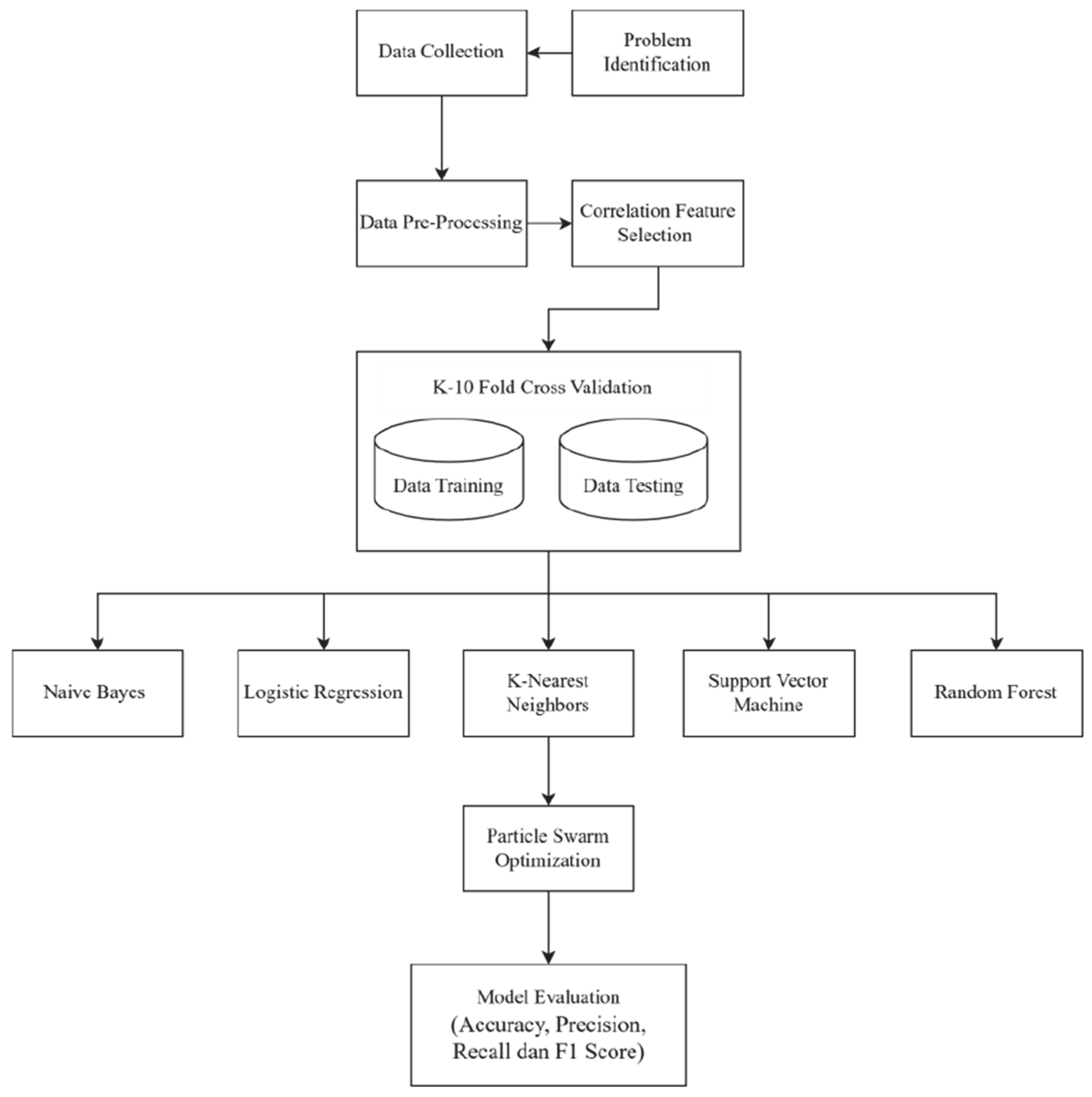
Figure 1 illustrates the research flowchart, outlining the primary stages of the process. The study begins with problem identification and data collection, followed by a pre-processing stage to ensure data quality. Subsequently, Correlation Feature Selection (CFS) is implemented to identify the most influential attributes for analysis. The dataset is then partitioned using the 10-fold cross-validation method into training and testing sets. These sets are used to build models based on two approaches: the standalone and the PSO-optimized versions of NB, LR, KNN, SVM, and RF. Finally, the performance of the five models is evaluated based on Accuracy, Precision, Recall, and F1-score.

2.3. Data Preprocessing

The pre-processing stage utilized a dataset consisting of 1025 rows, comprising 526 positive cases and 499 negative cases of heart disease. This stage involved two primary processes: selection and cleaning. The selection process aimed to identify relevant data aligned with the research objectives, while the cleaning phase addressed missing values, duplicates, and inconsistencies to maintain data integrity.

2.3.1. Data Cleaning

Data cleaning is a critical stage in rectifying or removing incomplete, inconsistent, or irrelevant data to ensure the dataset is prepared for analysis. In this study, the cleaning process specifically involved the removal of duplicate records to maintain the robustness of the experimental results [25]. The Zenodo version of the dataset contains synthetic duplicated samples that may introduce data leakage and lead to overly optimistic performance. Therefore, duplicate removal was performed to restore the dataset to its original UCI Cleveland size (302 records). Duplicate samples were identified using an exact matching rule across all feature attributes, where records with identical values in all clinical variables were detected and removed. After the deduplication process, the dataset was examined to ensure that the class distribution and overall feature statistics remained consistent with the original dataset, thereby minimizing the risk of dataset shift and ensuring unbiased model evaluation.anaina.

2.3.2. Data Standardization

The subsequent process involves standardization using the StandardScaler model. This technique aims to scale each numerical feature to achieve a mean of approximately zero and a standard deviation of one. This approach is implemented to normalize the value ranges across attributes, ensuring that differences in units do not lead to the dominance of specific features. By achieving a more centered and balanced data distribution, each variable can contribute proportionally to the model’s learning process [26,27].

$$x^{\prime }={\displaystyle \frac{x-\mathsf{\mu }}{\mathsf{\sigma }}}$$

(1)

In this process, x represents the input data to be normalized, μ is the mean value of the entire dataset, and σ denotes the standard deviation, which indicates the extent of data dispersion. Through this calculation, each data point is converted to a new scale with a mean of 0 and a standard deviation of 1.

2.4. Correlation Feature Selection

Correlation Feature Selection (CFS) is a data exploration technique used to identify the strength and direction of linear relationships between attributes. The correlation coefficients range from −1 to 1, representing positive, negative, or no correlation. This mechanism facilitates a deeper understanding of underlying patterns and helps identify potential redundancy among variables [28].

$$Cor{r}_{x,y}={\displaystyle \frac{\sum \left(x_i-\overline{x}\right)\left(y_i-\overline{y}\right)}{\sqrt{\sum {\left(x_i-\overline{x}\right)}^2{\left(y_i-\overline{y}\right)}^2}}}$$

(2)

The notation in the correlation formula indicates that Corr_x,y represents the correlation value between the feature attribute x and the target attribute y. The symbol x_i denotes the value of attribute x for the i-th data point, while y_i represents the value of the target attribute for the i-th data point. The symbols $\overline{x}$ and $\overline{y}$ respectively represent the mean values of all data points for attribute x and target y. Meanwhile, the symbol ∑ indicates the summation process over all data points in the dataset used in the correlation calculation.

2.5. 10-Fold Cross-Validation

Data splitting was performed using the K-Fold Cross-Validation method with a K value of 10. Although the K value can vary, K = 10 was chosen because it provides a good balance between bias and variance, keeps the proportion of training and testing data optimal, and results in more stable performance evaluation compared to K values that are too small or too large [29]. With the way it works, dividing the data in each iteration, the data division adjusts to the number of rows in the dataset [30].

2.6. Naive Bayes

Naive Bayes is a classification algorithm that works by calculating the probability of data based on its attribute values. In the Naive Bayes classification process, a large amount of training data is not required to obtain accurate parameter estimates [31]. Model Gaussian Naive Bayes, which is a variant of Naive Bayes used for numerical or continuous data. Gaussian Naive Bayes assumes that each feature follows a normal (Gaussian) distribution within each class [32]. Particle Swarm Optimization (PSO) was applied to optimize the var_smoothing hyperparameter of the Gaussian Naive Bayes model. In this case, each particle represents a candidate value of the var_smoothing parameter, and the PSO search space was defined within a predefined range to identify the optimal smoothing value that maximizes classification performance. Model performance was evaluated using 10-fold cross-validation, and the reported results represent the average accuracy across folds. The improvements observed after PSO were consistently observed across folds, indicating that the optimization contributes to improved model performance rather than minor fluctuations.

2.7. Logistic Regression

Logistic regression is used to model and estimate the relationship between a single binary dependent variable, often called the outcome, and one or more independent variables, known as covariates [33]. The logit transformation of the variable is converted into a probability with a range of 0 to 1 [34]. Optimized the regularization parameter (C), which controls the trade-off between model complexity and overfitting. Proper tuning of this parameter helps achieve better decision boundaries and improves predictive performance.

2.8. K-Nearest Neighbors

The KNN algorithm is one of the algorithms used for classifying a dataset. The KNN algorithm classifies objects based on the value of k or the nearest neighbors [35]. Optimized the number of nearest neighbors (k). Selecting an appropriate k value is crucial, as small values may lead to overfitting while large values may reduce model sensitivity.

2.9. Support Vector Machine

Support Vector Machine (SVM) is a machine learning algorithm that operates on the principle of Structural Risk Minimization (SRM) with the goal of finding the best hyperplane (separator) that separates two classes in the input space using the concept of the Support Vector Machine (SVM) model [36]. Optimized both the penalty parameter (C) and the kernel parameter (gamma). These parameters directly influence the margin width and the shape of the decision boundary, making them critical for achieving optimal classification results.

2.10. Random Forest

Random Forest is a type of decision tree built from arithmetic samples, but it has the ability to recognize different nodes. This model works by using a specific subset of features at each point, then determining the best boundary to use when analyzing the data. As a result, there will be many trees trained more thoroughly, and each will produce different predictions [37]. Optimized the number of trees (n_estimators). Increasing the number of trees generally enhances model stability and robustness, while excessive values may increase computational cost without significant performance gain.

2.11. Particle Swarm Optimization (PSO)

PSO involves controlling the algorithm’s velocity, which is an important aspect because it is the main mechanism that guides particle movement in the process of finding the optimal solution. Eberhart applied a maximum velocity limit and evaluated the results for various values of the k-th particle’s velocity in the swarm, which was then updated in the (i + 1) [38].

$$V_k\left(i+1\right)=V_k\left(i\right)+c_1{r}_1\left(p_{best,i}^k-X_k\left(i\right)\right)+c_2{r}_2\left(g_{best,i}-X_k\left(i\right)\right)$$

(3)

$$X_k\left(i+1\right)=X_k\left(i\right)+V_k\left(i+1\right)$$

(4)

In the Particle Swarm Optimization (PSO) algorithm, Vk(i) represents the velocity of the k-th particle at iteration i, while V_k(i + 1) is the updated velocity in the next iteration. The particle’s position is denoted by X_k(i), whereas $p_{best,i}^k$ represents the best position ever achieved by that particle and $g_{best,i}$ is the global best position among all particles. The parameters c₁ and c₂ function as acceleration constants, while r₁ and r₂ are random numbers in the range [0, 1] to introduce stochastic variation. The particle position is then updated using Equation (4). To ensure reproducibility and a fair performance comparison, the Particle Swarm Optimization (PSO) algorithm was implemented under fixed experimental settings. The swarm consisted of 20 particles and a maximum of 30 iterations. The inertia weight (w) was set to 0.7 to maintain a balance between exploration and exploitation, while the cognitive and social acceleration coefficients were set to c₁ = 1.5 and c₂ = 1.5, respectively. Each particle represented a candidate solution within the predefined search space, and the fitness function was defined as the average F1-score obtained through 10-fold cross-validation. The F1-score was selected as the fitness metric because it provides a balanced evaluation of precision and recall, which is particularly important in medical classification tasks where both false positives and false negatives must be carefully considered. Therefore, compared with accuracy, the F1-score was regarded as a more appropriate metric for evaluating classification performance in this study. The optimization process was conducted to identify the parameter configuration that maximized the overall classification performance. To ensure consistency, the evaluation procedure was applied uniformly across all cross-validation folds. Furthermore, the use of a fixed random seed and repeated experiments across PSO parameter settings, including w, c₁, and c₂, helped reduce the influence of stochastic variation and improve the reproducibility of the obtained results.

2.12. Evaluation Metrics

Evaluation is the process of measuring the accuracy of the results from a classification algorithm model implemented using the Confusion Matrix technique. The Confusion Matrix is used to measure the performance of the model by calculating the values of Accuracy, Precision, Recall, and F1-Score [39].

A confusion matrix is an evaluation method used to assess the performance of a classification model by comparing predicted results against data from rows representing actual classes and columns representing predicted classes [40]. The model’s performance is evaluated to assess its accuracy level and the quality of learning from the training data used by measuring the model’s performance as illustrated in

Table 1. Confusion Matrix.

	Prediction Positive	Prediction Negative
Class Positive	TP	FN
Class Negative	FP	TN

[41].

True Positive (TP) is the number of positive data points that the model successfully predicts as positive. True Negative (TN) is the number of negative data points correctly predicted as negative. False Positive (FP) indicates negative data incorrectly predicted as positive, while False Negative (FN) is positive data incorrectly predicted as negative. These four components are used in the confusion matrix to evaluate the performance of classification models, particularly in calculating metrics such as accuracy, precision, recall, and F1-score.

Accuracy is the ratio of the number of correctly predicted samples to the total number of samples in the test data, but it can be misleading if the class proportions are imbalanced because the model might achieve high accuracy simply by always predicting the majority class. The accuracy value ranges from 0 to 1, where a value of 1 indicates that all positive and negative data are correctly predicted, while a value of 0 means that no predictions are correct [42].

$$Accuracy={\displaystyle \frac{TP+TN}{TP+FP+TN+FN}}$$

(5)

Precision is used to measure the amount of data successfully predicted as positive, compared to all data predicted as positive [43]. Defined as the ratio between true positives and all positive predictions, a high precision value indicates that the model has few false positives, resulting in more accurate positive predictions [44].

$$Precision={\displaystyle \frac{TP}{TP+FP}}$$

(6)

Recall measures a model’s ability to correctly identify positive instances. It is calculated as the ratio of correctly predicted positive samples to the total number of actual positive samples [45].

$$Recall={\displaystyle \frac{TP}{TP+FN}}$$

(7)

The F1-Score is the harmonic mean of precision and recall, balancing both so that extreme values in one will lower the score. This metric depends on the determination of positive and negative classes. If the model is biased toward the majority class, the F1-score can appear high, but if the labels are reversed, the value can be low even with the same data distribution. This score ranges from 0 to 1, with 1 meaning perfect precision and recall, while 0 means that both fail [46].

$$F1-Score=2\times {\displaystyle \frac{ Recall\times Presisi}{Recall+Presisi}}$$

(8)

3. Results

This section discusses the results of applying the hybrid PSO and correlation-based feature selection model to the NB, LR, KNN, SVM, and RF algorithms, along with an analysis of their performance using Accuracy, Precision, Recall, and F1-Score metrics. The evaluation results are used to assess the effectiveness and limitations of each model in classifying heart disease data.

3.1. Dataset Overview

Table 2. Dataset Heart Disease.

No	Age	Sex	Cp	Trestbps	Chol	Fbs	Restecg	Thalach	Exang	Oldpeak	Slope	Ca	Thal	Target
1	52	1	0	125	212	0	1	168	0	1	2	2	3	0
2	53	1	0	140	203	1	0	155	1	3.1	0	0	3	0
3	70	1	0	145	174	0	1	125	1	2.6	0	0	3	0
4	61	1	0	148	203	0	1	161	0	0	2	1	3	0
5	62	0	0	138	294	1	1	106	0	1.9	1	3	2	0
…	…	…	…	…	…	…	…	…	…	…	…	…	…	…
1021	59	1	1	140	221	0	1	164	1	0	2	0	2	1
1022	60	1	0	125	258	0	0	141	1	2.8	1	1	3	0
1023	47	1	0	110	275	0	0	118	1	1	1	1	2	0
1024	50	0	0	110	254	0	0	159	0	0	2	0	2	1
1025	54	1	0	120	188	0	1	106	0	1.4	1	1	3	0

presents the dataset obtained from the Zenodo platform, which is used for heart disease analysis with features including Age, Sex, Chest Pain Type, TrestBPS, Cholesterol, FastingBS, Resting Electrocardiographic Results, Thalach (Maximum Heart Rate Achieved), Exang, Oldpeak, Slope, Ca (Number of Major Vessels), and Thalassemia. The last column represents the target variable, indicating the diagnostic outcome, where a value of 1 denotes that the patient has heart disease and 0 indicates otherwise. Overall, this dataset is used to examine the relationship between health-related factors and the likelihood of being diagnosed with heart disease. Prior to further analysis, the data undergoes a preprocessing stage.

3.2. Results of Data Preprocessing

3.2.1. Summary of Data Cleaning Results

The data cleaning process is summarized in

Table 3. Data Cleaning Results.

Initial Dataset Size	Duplicate Records	Final Records After Cleaning
1025	723	302

.

The table above represents a summary of the vital steps in the data preprocessing stage, particularly in the data validity assurance procedure through deduplication. From a total of 1025 rows of raw data collected, a substantial elimination of 723 duplicate samples was performed, resulting in a highly concise yet information-dense final dataset consisting of 302 rows.

3.2.2. Results of Data Standardization

Each attribute is transformed into a scale with a mean close to zero and a standard deviation of one, resulting in data values distributed across both positive and negative ranges. Negative values indicate that the data points are below the mean, while positive values indicate that they are above the mean, with the magnitude of the values representing the distance from the center of the distribution.

3.3. Correlation Feature Selection Results

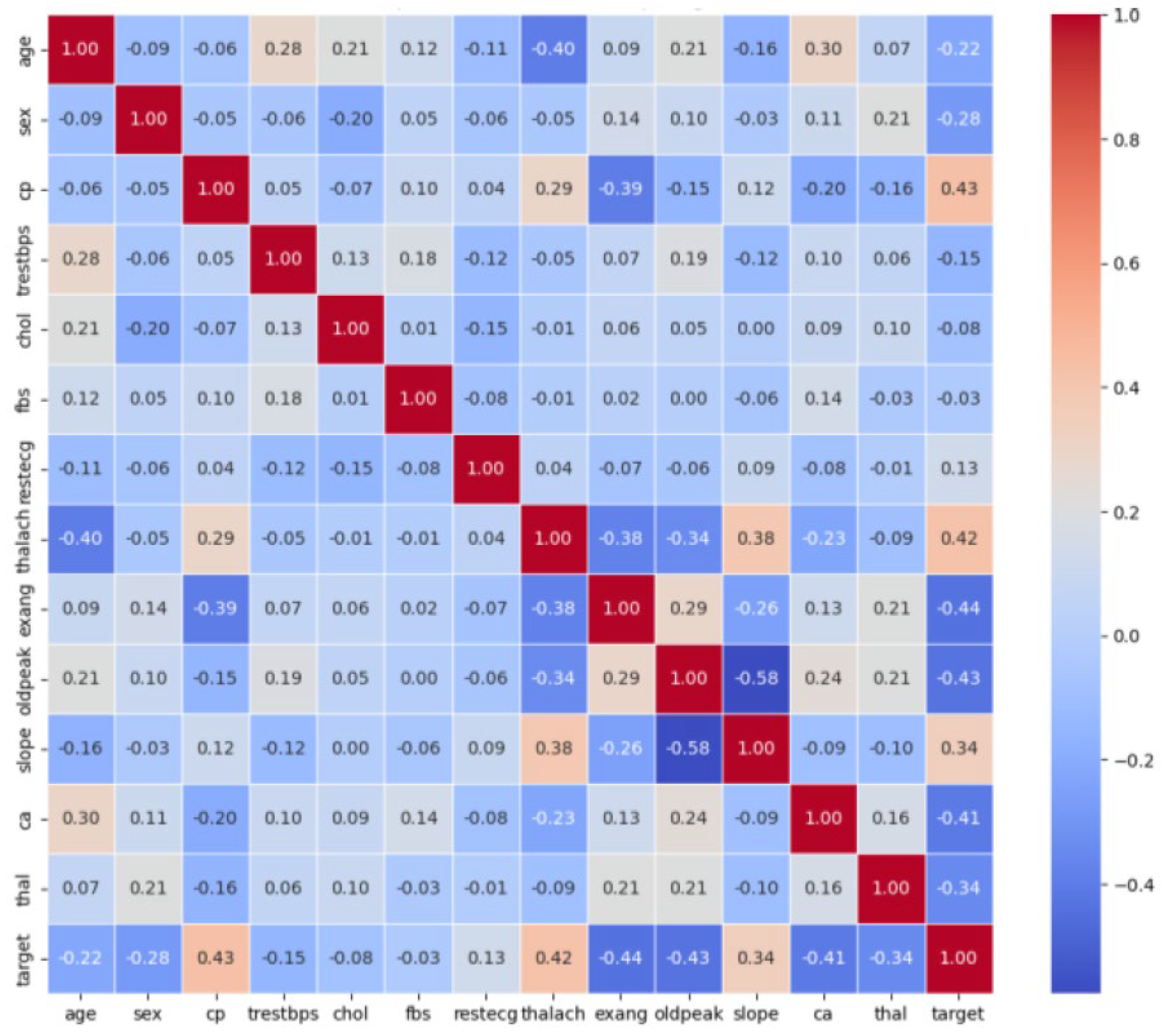
The correlation heatmap of all dataset attributes is presented in Figure 2. Based on the correlation heatmap analysis, several attributes show relatively strong relationships with the target variable.

Based on the correlation heatmap analysis, several attributes show relatively strong relationships with the target variable. The attributes cp (0.432080) and thalach (0.419955) have the highest positive correlations, indicating that increases in these attributes tend to be associated with a higher likelihood of heart disease. In contrast, exang (−0.435601), oldpeak (−0.429146), and ca (−0.408992) show relatively strong negative correlations, indicating inverse relationships with the target variable. Meanwhile, fbs (−0.026826) exhibits the lowest correlation value among all features, indicating a very weak linear relationship with the target variable. Therefore, it was identified as a candidate for elimination based on relative comparison rather than a fixed threshold. However, a low linear correlation does not necessarily imply a lack of predictive contribution, as features may still provide useful information through non-linear relationships or interactions, particularly in models such as Random Forest and SVM. The results of the Correlation Feature Selection process are presented in

Table 4. Dataset Correlation Feature Selection.

No	Age	Sex	Cp	Trestbps	Chol	Restecg	Thalach	Exang	Oldpeak	Slope	Ca	Thal	Target
1	−0.267966	1	0	−0.376556	−0.667728	1	0.806035	0	−0.037124	2	2	3	0
2	−0.157260	1	0	0.478910	−0.841918	0	0.237495	1	1.773958	0	0	3	0
3	1.724733	1	0	0.764066	−1.403197	1	−1.074521	1	1.342748	0	0	3	0
4	0.728383	1	0	0.935159	−0.841918	1	0.499898	0	−0.899544	2	1	3	0
5	0.839089	0	0	0.364848	0.919336	1	−1.905464	0	0.739054	1	3	2	0

. The results of the Correlation Feature Selection process are presented in Table 4.

The table above shows the results of the Correlation Feature Selection process, where the fbs attribute has a correlation value close to zero, indicating a very weak relationship with the target variable and is therefore considered less informative. Based on these results, 13 attributes, including the target feature, are used for data splitting and model development.

3.4. 10-Fold Cross-Validation Results

The dataset was evaluated using the 10-Fold Cross-Validation technique on a dataset consisting of 302 samples. Since the total number of samples cannot be evenly divided into ten folds, slight variations occur in the number of training and testing data across folds, where the training set ranges from 271 to 272 samples and the testing set consists of 30 to 31 samples.

3.5. Performance Comparison of Classification Algorithms

To provide a fair evaluation of the proposed optimization strategy, the initial performance of all classification algorithms was first measured without applying Particle Swarm Optimization (PSO). This baseline experiment aims to reflect the original capability of each classifier using default or manually selected parameters, serving as a reference for comparison with the optimized models. The evaluation was conducted using 10-fold cross-validation and assessed based on accuracy, precision, recall, and F1-score. The baseline results for Naive Bayes, Logistic Regression, K-Nearest Neighbor, Support Vector Machine, and Random Forest are presented in

Table 5. Comparison of Classification Algorithms from Baseline.

Model	Accuracy	Precision	Recall	F1-Score
Naive Bayes (NB)	81.49%	82.57%	84.38%	83.00%
Logistic Regression (LR)	82.47%	80.31%	88.56%	84.10%
K-Nearest Neighbor (KNN)	81.16%	77.51%	90.94%	83.48%
Support Vector Machine (SVM)	82.80%	79.31%	91.70%	84.88%
Random Forest (RF)	82.80%	83.62%	86.07%	84.46%

.

After establishing the baseline performance, PSO was applied to optimize model parameters and feature subsets for each classifier. The optimized results demonstrate the effectiveness of PSO in enhancing classification performance. The comparison highlights improvements in predictive accuracy and overall model stability, as summarized in

Table 6. Comparison of Classification Algorithms: PSO.

Model	Accuracy	Precision	Recall	F1-Score
Naive Bayes (NB)	84.48%	82.37%	91.62%	86.33%
Logistic Regression (LR)	84.45%	81.74%	91.01%	85.98%
K-Nearest Neighbor (KNN)	82.81%	79.02%	92.13%	84.84%
Support Vector Machine (SVM)	84.46%	80.54%	92.72%	86.04%
Random Forest (RF)	84.11%	81.93%	92.21%	86.35%

.

To provide a fair evaluation of the proposed method, the classification performance of all models was first assessed using baseline settings without Particle Swarm Optimization (PSO). These baseline results represent the original capability of each classifier before any optimization process was applied. The evaluation was conducted using 10-fold cross-validation and measured in terms of accuracy, precision, recall, and F1-score.

After establishing the baseline performance, PSO combined with correlation-based feature selection was applied to optimize model parameters and feature subsets. The optimized classification performance of the five algorithms is presented in Table 6. The results are reported as the average values across all folds.

Overall, all algorithms demonstrate comparable performance after optimization, with accuracy values ranging from 82.81% to 84.48%. The highest accuracy is achieved by Naive Bayes (84.48%), followed closely by Support Vector Machine (84.46%) and Logistic Regression (84.45%). Random Forest obtains an accuracy of 84.11%, while K-Nearest Neighbor shows the lowest accuracy at 82.81%. In terms of precision, Naive Bayes achieves the highest value (82.37%), whereas K-Nearest Neighbor records the lowest precision at 79.02%. Logistic Regression, Support Vector Machine, and Random Forest produce similar precision values of 81.74%, 80.54%, and 81.93%, respectively.

Regarding recall, all models exhibit high values above 91%, indicating a strong capability to correctly identify patients with heart disease. The highest recall is obtained by Support Vector Machine (92.72%), followed by Random Forest (92.21%) and K-Nearest Neighbor (92.13%). Naive Bayes and Logistic Regression achieve recall values of 91.62% and 91.01%, respectively. The F1-score, which represents the balance between precision and recall, shows that Random Forest achieves the highest value (86.35%), followed by Naive Bayes (86.33%) and Support Vector Machine (86.04%). Logistic Regression and K-Nearest Neighbor obtain F1-scores of 85.98% and 84.84%, respectively.

3.6. Confusion Matrix Analysis

The baseline confusion matrices of all classifiers are presented in the first row of Figure 3. Overall, the models demonstrate reasonable classification capability, as indicated by a higher number of correctly classified instances (true positives and true negatives) compared to misclassifications. However, several false positives and false negatives are still observed across all algorithms. Naive Bayes and Logistic Regression show moderate misclassification rates, while K-Nearest Neighbor and Support Vector Machine exhibit relatively higher false predictions. Random Forest provides comparatively balanced results but still produces some incorrect classifications. These errors indicate that the baseline models have not yet achieved optimal decision boundaries, which may limit diagnostic reliability, particularly in detecting positive heart disease cases.

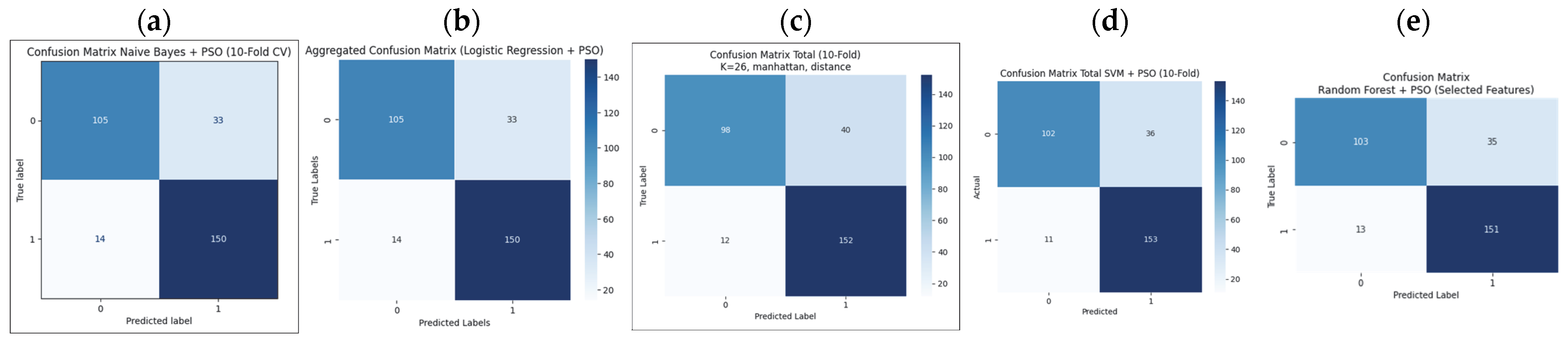
The PSO-optimized confusion matrices are shown in the second row of Figure 4. After applying Particle Swarm Optimization and correlation-based feature selection, all classifiers exhibit noticeable improvements. The number of correctly classified samples increases, while false positives and false negatives decrease compared to the baseline configuration. Naive Bayes shows fewer misclassified instances, indicating improved feature relevance. Logistic Regression and Support Vector Machine demonstrate clearer decision boundaries with reduced error counts. K-Nearest Neighbor achieves more stable predictions, and Random Forest presents the most balanced confusion matrix with minimal misclassification. The reduction in false negatives is particularly important for medical diagnosis, as it minimizes the risk of failing to detect patients with heart disease. These findings confirm that PSO effectively enhances classification reliability and overall predictive performance.

4. Conclusions and Recommendations

This study demonstrates that the integration of Correlation Feature Selection (CFS) and Particle Swarm Optimization (PSO) provides competitive and consistent classification performance for heart disease detection. To ensure a fair evaluation, baseline models were first tested without optimization, followed by PSO-based parameter tuning and feature subset selection. The experimental results indicate that the optimized models consistently outperform the baseline configurations across all evaluation metrics, confirming the effectiveness of the proposed optimization strategy. Based on 10-fold cross-validation, the classification accuracy ranges from 82.81% to 84.48%, with Naive Bayes achieving the highest accuracy. In terms of precision, the highest value of 82.37% is obtained by Naive Bayes, while K-Nearest Neighbor records the lowest precision of 79.02%. Regarding recall, Support Vector Machine attains the highest value of 92.72%, whereas Logistic Regression shows the lowest recall at 91.01%. Furthermore, Random Forest achieves the highest F1-score of 86.35%, indicating a balanced trade-off between precision and recall.

Overall, the results confirm that the combination of feature selection and PSO not only improves predictive accuracy but also enhances model stability and generalization capability. Therefore, the proposed hybrid framework shows strong potential to be implemented as a reliable decision support system for early and accurate heart disease diagnosis. Future studies are recommended to employ larger and more diverse datasets to further enhance model generalization capability. Feature selection and optimization methods may also be combined or compared with other techniques to obtain a more optimal classification performance. In addition, the developed model can be integrated into a decision support system to enable direct utilization in early heart disease detection.