Multi-Orbit, Multi-Resolution Earth Observation for Intelligent Target Scheduling ^†

Abstract

The growing demand for accurate and timely Earth observation (EO) data has made autonomous mission planning increasingly essential. In particular, data acquisition planning has gained attention in recent years with the advent of agile Earth observation satellites (AEOSs). This process involves two main stages: target identification and observation scheduling. Traditionally, the former is performed manually, while the latter requires solving the agile Earth observation satellite scheduling problem (AEOSSP), a complex combinatorial optimization problem. In this work, we propose a constellation design comprising EO satellites deployed in medium Earth orbit (MEO) and low Earth orbit (LEO). The MEO satellites acquire low-resolution (LR) images for onboard target identification and subsequently schedule high-resolution (HR) observations by a set of LEO AEOSs. We adapt the AEOSSP to this multi-orbit context by explicitly considering communication constraints between MEO and LEO satellites and propose several heuristic solution methods. Among them, the quality-based greedy algorithm yields up to a 35.5% improve in observation profit in simple, low-conflict scenarios, while the structured heuristic algorithm proves the most robust, achieving up to a 21.5% increase in challenging schedules.

1. Introduction

Earth observation (EO) is a long-standing satellite application that provides unique insights into climate change monitoring, disaster management, and urban mapping, among others. Consequently, the demand for accurate and timely EO data is continuously growing, driving advances in the processing, communication, and maneuvering capabilities of Earth observation satellites (EOSs) [1,2]. Together with recent breakthroughs in Artifical Intelligence (AI) and Machine Learning (ML), these improvements enable autonomous mission planning, which is essential to meet increasing requirements for responsiveness, revisit frequency, and quality.

Designing autonomous satellite constellations must consider factors such as orbital altitude, which strongly influences system performance [3]. Geostationary orbit (GEO) and medium Earth orbit (MEO) satellites offer broad coverage and wide-swath imagery suitable for environmental monitoring, but their altitude limits imaging resolution and causes long propagation delays and signal attenuation. In contrast, low Earth orbit (LEO) constellations offer short propagation delays, low signal attenuation, and high-resolution (HR) but narrow-swath imaging capabilities, making them attractive for EO tasks. Recent research advocates combining satellites at different altitudes within the same system, with higher-altitude satellites serving as mission planners [4,5] and lower-altitude ones handling execution and local planning.

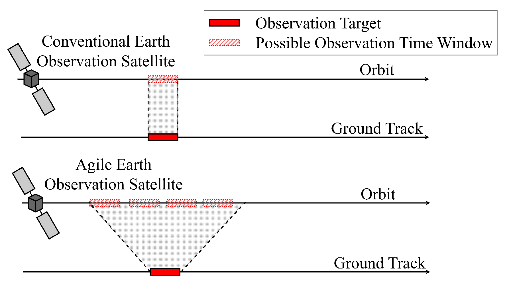
Among the various aspects of mission planning, data acquisition (i.e., image capture) has become one of the most extensively studied topics in recent years. This interest is driven by the advent of agile Earth observation satellites (AEOSs) [2], which, unlike conventional EOSs, feature three-axis attitude maneuver control (roll, pitch, and yaw). This functionality extends the visible time windows (VTWs)—the intervals during which a target can be observed—thus enabling multiple observation time windows (OTWs), hereafter referred to as actual observation intervals, for a single target (see Figure 1). While this flexibility increases the number of feasible schedules, it also complicates the OTW selection when there are multiple targets within the same scheduling time horizon (STH). This challenge, known as the agile Earth observation satellite scheduling problem (AEOSSP), consists of determining the target sequence, the OTW for each target, and the AEOS responsible for execution when multiple AEOSs are available. The goal is to maximize the total observation profit—a metric that quantifies the value of an observation, defined according to the application—while satisfying a set of operational constraints. Because the AEOSSP is NP-hard, exact methods quickly become impractical for large-scale instances, and heuristic, metaheuristic [6,7], or ML-based approaches [4] are typically adopted when rapid, efficient solutions are required. Several studies address the AEOSSP from an autonomous perspective. For instance, ref. [4] considers a scenario in which a high-orbit EOS captures low-resolution (LR) images to detect targets and centrally schedules observations for an LEO constellation, assuming persistent communication. Similarly, ref. [8] proposes a bi-satellite cluster where a leading autonomous EOS collects LR, wide-swath images to identify targets, while an AEOS acquires HR imagery for their recognition.

In this work, we propose an autonomous EO constellation design with EOSs deployed at two orbital layers: MEO and LEO. MEO EOSs capture LR images and process them onboard to detect and classify targets into priority levels according to their predicted urgency. Once targets are identified, each MEO EOS schedules their HR observation by a set of LEO AEOSs with the objective of maximizing the total observation profit, defined in terms of target priority and image quality. Performing such scheduling requires solving the AEOSSP after completing the target identification stage. This framework entails two main challenges. The first is communication between the two orbital layers: since LEO AEOSs are not always within the coverage area of the MEO EOSs, the corresponding communication time windows (CTWs) must be incorporated into the problem formulation. All scheduled OTWs for a given AEOS must occur only after receiving the scheduling instructions. The second challenge concerns timely and efficient schedule generation. CTWs between MEO and LEO satellites are limited, constraining opportunities to transmit instructions, and lengthy scheduling processes may result in missed opportunities given the high orbital velocity of LEO satellites. This is further compounded by the need to minimize energy consumption in space operations [9] and the limited onboard processing capacity. The first challenge is addressed by adapting the AEOSSP to the proposed framework, while the second is tackled through the use of lightweight heuristic algorithms.

The remainder of this paper is organized as follows. Section 2 presents the system model, while Section 3 describes the AEOSSP. Section 4 introduces the heuristic methods, and Section 5 reports the results. Finally, Section 6 concludes the paper.

2. System Model

To address this challenging AEOSSP, we adopt the following assumptions. The computational complexity of the target identification algorithm is set to the worst-case execution time, ensuring that all OTWs remain feasible after its execution. We consider only point targets observable within a single pass. Each EOS in the constellation is assumed to have sufficient energy to perform all required operations. Onboard processing and downlink of HR images to the ground segment are not considered.

The first subset of EOSs, denoted by M, comprises the MEO EOSs. Each EOS $m\in M$ operates at altitude $h_m$ with orbital inclination ${\iota }_m$ and is equipped with onboard Central Processing Units (CPUs) to process the acquired data. EOS m maintains a fixed attitude and, at time ${\tau }_m^{\left(cap\right)}$, captures an LR image for target identification; the capture time is considered negligible. To avoid conflicts, images from different MEO EOSs are assumed not to overlap, ensuring maximum coverage. Each image spans the same ground area A, with a spatial resolution determined by the ground sample distance (GSD), the average ground distance per pixel. Given the GSD and the bit depth per pixel $q_{px}$, the image size in bits is

$$D={\displaystyle \frac{q_{px}·A}{GS{D}^2}}.$$

(1)

To identify the targets, an algorithm with fixed complexity C, expressed in CPU cycles per bit, is applied. Thus, the processing time required by EOS m to analyze the acquired data is

$${\tau }_m^{\left(proc\right)}={\displaystyle \frac{D·C}{N_{cores}·f_{CPU}}},$$

(2)

where $N_{cores}$ denotes the number of CPU cores and $f_{CPU}$ their work frequency.

The set of targets identified by m is denoted as $T_m$, where each target $t_m\in T_m$ is associated with an integer value ${\rho }_{t_m}$ representing its priority level. Once the targets have been identified, each MEO EOS m schedules their observation during an $STH=[st{h}_a,st{h}_b]$ by the second subset of satellites, denoted by S, which comprises the LEO AEOSs. The time available for scheduling the observation is denoted as ${\tau }_m^{\left(sch\right)}$. Each AEOS $s\in S$ operates at altitude $h_s$ and an orbital inclination ${\iota }_s$. The MEO EOSs are assumed to have knowledge of the positions, trajectories, and instrumentation of the LEO AEOSs, allowing them to estimate their VTWs with respect to the identified targets, along with the corresponding CTWs. Each target $t_m$ requires an observation time ${\tau }_{t_m}^{\left(obs\right)}$ and may be observed by AEOS s across multiple orbital passes. Let $O_{s,t_m}$ denote the set of orbits in which AEOS s can observe target $t_m$. For each orbit $o\in O_{s,t_m}$, the VTW is defined as $VT{W}_{s,t_m,o}=[s{w}_{s,t_m,o},e{w}_{s,t_m,o}]$, where $s{w}_{s,t_m,o}$ and $e{w}_{s,t_m,o}$ are the start and end times, respectively. Each $VT{W}_{s,t_m,o}$ is discretized into a set of OTWs with a fixed step size of $prc$ seconds. Thus, $OT{W}_{s,t_m,o,w}$ denotes the OTW for satellite s and target $t_m$ during orbit o within $VT{W}_{s,t_m,o}$, with index $w\in W_{s,t_m,o}^{\left(obs\right)}$, where $W_{s,t_m,o}^{\left(obs\right)}$ is the set of OTWs in $VT{W}_{s,t_m,o}$. Each $OT{W}_{s,t_m,o,w}$ is defined by $[s{o}_{s,t_m,o,w},e{o}_{s,t_m,o,w}]$ and is associated with an observation profit ${\sigma }_{s,t_m,o,w}$, where $s{o}_{s,t_m,o,w}$ and $e{o}_{s,t_m,o,w}$ are the start and end times determined by the required observation time ${\tau }_{t_m}^{\left(obs\right)}$.

The attitude required for an AEOS s to observe a target $t_m$ during $OT{W}_{s,t_m,o,w}$ is defined by its roll, pitch, and yaw angles, denoted by ${\theta }_{s,t_m,o,w}$, ${\varphi }_{s,t_m,o,w}$ and ${\psi }_{s,t_m,o,w}$, respectively. The maneuverability of an AEOS is constrained by the maximum roll, pitch, and yaw angles (${\theta }_{\max }$, ${\varphi }_{\max }$, and ${\psi }_{\max }$), and by the sensor’s slewing speed. Typically, the attitude transition time between two consecutive observations is modeled as a piecewise linear function [10]:

$$\mathrm{\Delta }{\tau }_{t_m,w-t_m^{\prime },w^{\prime }}=\left\{\begin{array}{cc}11.66,\hfill & {\alpha }_{t_m,w-t_m^{\prime },w^{\prime }}\le {10}^{\circ }\hfill \\ 5+{\alpha }_{t_m,w-t_m^{\prime },w^{\prime }}/1.5,\hfill & {10}^{\circ }<{\alpha }_{t_m,w-t_m^{\prime },w^{\prime }}\le {30}^{\circ }\hfill \\ 10+{\alpha }_{t_m,w-t_m^{\prime },w^{\prime }}/2,\hfill & {30}^{\circ }<{\alpha }_{t_m,w-t_m^{\prime },w^{\prime }}\le {60}^{\circ }\hfill \\ 16+{\alpha }_{t_m,w-t_m^{\prime },w^{\prime }}/2.5,\hfill & {60}^{\circ }<{\alpha }_{t_m,w-t_m^{\prime },w^{\prime }}\le {90}^{\circ }\hfill \\ 22+{\alpha }_{t_m,w-t_m^{\prime },w^{\prime }}/3,\hfill & {\alpha }_{t_m,w-t_m^{\prime },w^{\prime }}>{90}^{\circ }\hfill \end{array}\right.,$$

(3)

$${\alpha }_{t_m,w-t_m,w^{\prime }}=|{\theta }_{s,t_m,o,w}-{\theta }_{s,t_m^{\prime },o,w^{\prime }}|+|{\varphi }_{s,t_m,o,w}-{\varphi }_{s,t_m^{\prime },o,w^{\prime }}|+|{\psi }_{s,t_m,o,w}-{\psi }_{s,t_m^{\prime },o,w^{\prime }}|,$$

(4)

where ${\alpha }_{t_m,w-t_m^{\prime },w^{\prime }}$ is the total attitude transition angle between the observation of $OT{W}_{s,t_m,o,w}$ and $OT{W}_{s,t_m^{\prime },o,w^{\prime }}$.

Once the observations have been scheduled, the corresponding instructions are transmitted to the AEOSs after a time ${\tau }_{m,s}^{\left(store\right)}$, representing the elapsed time between schedule generation onboard EOS m and its transmission to AEOS s. This transmission must occur within one of the available CTWs, so that ${\tau }_{m,s}^{\left(\mathrm{store}\right)}$ can vary for each satellite pair $(m,s)$. Let $W_{m,s}^{\left(com\right)}$ denote the set of CTWs in which EOS m can establish a communication link with AEOS s. The n-th CTW for EOS m and AEOS s is defined as $CT{W}_{m,s}^n=[s{c}_{m,s}^n,e{c}_{m,s}^n]$, where $s{c}_{m,s}^n$ and $e{c}_{m,s}^n$ are the start and end times of the CTW, respectively. Propagation and transmission delays are considered when communicating these instructions. Thus, the time required to transmit the schedule from EOS m to AEOS s is calculated as

$${\tau }_{m,s}^{\left(com\right)}={\displaystyle \frac{D}{R_l}}+{\displaystyle \frac{d_{m,s}}{c}},$$

(5)

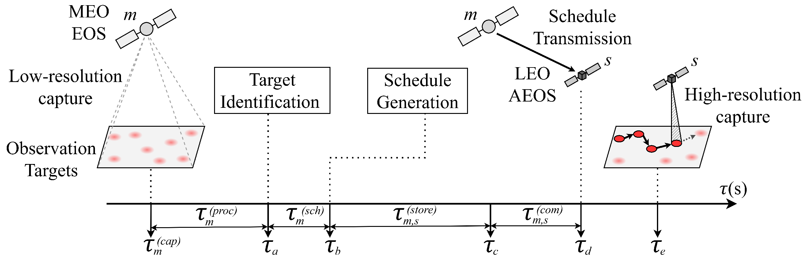
where $R_l$ is the bit rate of a given link l, $d_{m,s}$ the distance between EOS m and AEOS s, and c the speed of light. The complete task sequence is shown in Figure 2.

3. Agile Earth Observation Satellite Scheduling Problem

The AEOSSP is characterized by a demand for tasks that exceeds the capacity of the AEOSs. Moreover, when multiple AEOSs are involved, a single target may be observed by various AEOS, and together with the large number of available OTWs, this can significantly increase the complexity of the problem. The mathematical formulation is given below.

$$\max \sum _{s\in S}\sum _{t_m\in T_m}\sum _{o\in O_{s,t_m}}\sum _{w\in W_{s,t_m,o}}{\sigma }_{s,t_m,o,w}·x_{s,t_m,o,w},$$

(6)

This is subject to

$$s{w}_{s,t_m,o}\le s{o}_{s,t_m,o,w}\le e{o}_{s,t_m,o,w}\le e{w}_{s,t_m,o},$$

(7)

$$e{o}_{s,t_m,o,w}+\mathrm{\Delta }{\tau }_{t_m,w-t_m^{\prime },w^{\prime }}\le s{o}_{s,t_m^{\prime },o,w^{\prime }},$$

(8)

$$s{c}_{m,s}^n\le {\tau }_m^{\left(cap\right)}+{\tau }_m^{\left(proc\right)}+{\tau }_m^{\left(sch\right)}+{\tau }_{m,s}^{\left(store\right)}\le e{c}_{m,s}^n-{\tau }_{m,s}^{\left(com\right)},$$

(9)

$${\tau }_m^{\left(cap\right)}+{\tau }_m^{\left(proc\right)}+{\tau }_m^{\left(sch\right)}+{\tau }_{m,s}^{\left(store\right)}+{\tau }_{m,s}^{\left(com\right)}\le \min \left(S{O}_{m,s}\right),$$

(10)

$$\sum _{s\in S}\sum _{o\in O_{s,t_m}}\sum _{w\in W_{s,t_m,o}}{x}_{s,t_m,o,w}\le 1,x_{s,t_m,o,w}\in \{0,1\},$$

(11)

where ${\sigma }_{s,t_m,o,w}$ is the observation profit obtained from observing target $t_m$ during $OT{W}_{s,t_m,o,w}$; $x_{s,t_m,o,w}$ is a binary decision variable equal to 1 if $OT{W}_{s,t_m,o,w}$ is scheduled and 0 otherwise; and $S{O}_{m,s}$ denotes the set of scheduled OTWs start times for AEOS s by EOS m. Equation (6) defines the objective function, which maximizes the total observation profit; Equation (7) ensures that the observation of target $t_m$ occurs within one of its available VTWs; Equation (8) guarantees that $OT{W}_{s,t_m,o,w}$ and $OT{W}_{s,t_m^{\prime },o,w^{\prime }}$ can be scheduled consecutively, where $t_m^{\prime }$ is the target observed immediately after $t_m$; Equation (9) checks the feasibility of schedule data transmission; Equation (10) enforces that all scheduled observations for AEOS s occur only after receiving the scheduling instructions; and Equation (11) states that a target appears at most once in a single schedule.

The observation profit is defined considering both target priority and image spatial resolution during $OT{W}_{s,t_m,o,w}$, given by the GSD [11]. It is computed as

$${\sigma }_{s,t_m,o,w}={\rho }_{t_m}·{\displaystyle \frac{GS{D}_{nadir}}{GS{D}_{s,t_m,o,w}}},$$

(12)

where $GS{D}_{nadir}$ denotes the GSD at nadir, and $GS{D}_{s,t_m,o,w}$ the GSD of the captured image during $OT{W}_{s,t_m,o,w}$. The GSD increases as the target moves away from the nadir, and a small value leads to a better spatial resolution.

4. Heuristic Methods

Heuristic approaches typically rely on indicators to rank targets and OTWs, guiding the construction of the solution [6,7]. In this section, we present greedy-based heuristics for efficiently solving the AEOSSP. We first define a set of heuristic indicators that form the basis of the algorithms.

4.1. Heuristic Indicators

In addition to target priority and the GSD of the acquired image, which directly determine the observation profit, we introduce additional heuristic indicators to guide the decision-making process.

Targets differ in the number of scheduling opportunities available during an STH, as the number of feasible OTWs varies. We define the assignment flexibility of target $t_m$, denoted $F{L}_{t_m}$, as the number of its available OTWs. Higher $F{L}_{t_m}$ values indicate more opportunities for inclusion in the final schedule. This indicator can be used to normalize target priority, leading to the concept of target weight,

$$w_{t_m}={\displaystyle \frac{{\rho }_{t_m}}{F{L}_{t_m}}},$$

(13)

which accounts for both target priority and the difficulty of including it in the schedule.

Furthermore, once a target is scheduled, some OTWs may become infeasible due to the satellites’ attitude maneuver constraints. These OTWs are referred to as being in conflict. Hence, the number of conflicting OTWs can be incorporated into the scheduling process [7], complementing the previously defined target weight. If the number of conflicting OTWs is considered, we define the Conflict-Aware Count Factor (CACF):

$$CAC{F}_{t_m}=\left\{\begin{array}{cc}{\displaystyle \frac{w_{t_m}}{|COT{W}_{t_m}|}},\hfill & COT{W}_{t_m}\ne \varnothing \hfill \\ w_{t_m},\hfill & \mathrm{otherwise}\hfill \end{array}\right.,$$

(14)

where $COT{W}_{t_m}$ denotes the set of OTWs belonging to other targets that conflict with those of target $t_m$, and $|COT{W}_{t_m}|$ is its cardinality. Similarly, for a given $OT{W}_{s,t_m,o,w}$, we define the opportunity cost (OC) [6] as the sum of the observation profits of the conflicting OTWs:

$$O{C}_{s,t_m,o,w}=\sum _{t_m^{\prime },w^{\prime }\in COT{W}_{s,t_m,o,w}}{\sigma }_{s,t_m^{\prime },o,w^{\prime }},$$

(15)

where $COT{W}_{s,t_m,o,w}$ is the set of OTWs in conflict with $OT{W}_{s,t_m,o,w}$. Lower $O{C}_{s,t_m,o,w}$ values indicate smaller potential losses in the total observation profit if $OT{W}_{s,t_m,o,w}$ is scheduled.

4.2. Algorithms

We now present several greedy strategies for efficiently solving the AEOSSP. In all strategies, targets are ranked according to a given criterion and are considered in that order for scheduling. For each target, if feasible OTWs exist, one is selected for scheduling based on additional criteria; otherwise, the target is skipped. After scheduling an observation, the infeasible OTWs are removed, and the process continues until all targets have been evaluated. The strategies are as follows:

• First-In First-Out (FIFO) algorithm. Targets are scheduled in ascending VTW order, with each assigned to its first feasible OTW. This is a time-based greedy strategy that aims to maximize the number of captured targets, without considering target weight or image quality.
• Quality-based greedy algorithm. Targets are ranked by descending weight, and each is scheduled at the OTW with the lowest GSD, corresponding to the highest quality.
• Conflict-based greedy algorithm. Targets are ranked by descending CACF, and each is scheduled at the feasible OTW with the lowest OC.
• Structured heuristic algorithm. Targets are grouped according to ${\rho }_{t_m}$, with groups arranged in descending order of ${\rho }_{t_m}$. Within each group, targets are ranked by ascending $F{L}_{t_m}$, and each is scheduled at the feasible OTW with the lowest OC.

5. Results

The simulation setup is as follows. The MEO layer consists of two EOSs at $h_m=6000\mathrm{km}$ with an inclination ${\iota }_m={15}^{\circ }$, arranged in two orbital planes following a Walker delta topology with a ${180}^{\circ }$ phase shift. Each EOS has a CPU featuring $N_{cores}=8$ and work frequency $f_{CPU}=1.8$ GHz. LR images cover $A=9\times {10}^9{\mathrm{km}}^2$ with $GSD=100$ m/pixel, and the complexity of the target identification algorithm is set to $C=1000$ CPU cycles per bit, corresponding to the worst-case execution time. The available scheduling time is ${\tau }_m^{\left(sch\right)}=10$ s. We evaluate instances with {60, 80, 100, 120} targets, uniformly distributed across each LR image, with priorities ${\rho }_{t_m}\sim \mathcal{U}(1,5)$, observation times ${\tau }_{t_m}^{\left(obs\right)}\sim \mathcal{U}(1,5)\mathrm{s}$, and a discretization step of $prc=10$ s. The LEO AEOSs are deployed at $h_s=600\mathrm{km}$ with an inclination ${\iota }_s={53}^{\circ }$. Three LEO configurations are considered: (1) four AEOSs in four orbital planes, (2) eight AEOSs in four orbital planes, and (3) two AEOSs in two orbital planes, all arranged in a Walker delta topology. Camera attitude maneuvers are constrained by ${\theta }_{max}={45}^{\circ }$, ${\varphi }_{max}={45}^{\circ }$, and ${\psi }_{max}={90}^{\circ }$, with a nadir spatial resolution of $GS{D}_{nadir}=0.5$ m/pixel. We assume RF inter-satellite links with parameters from [12].

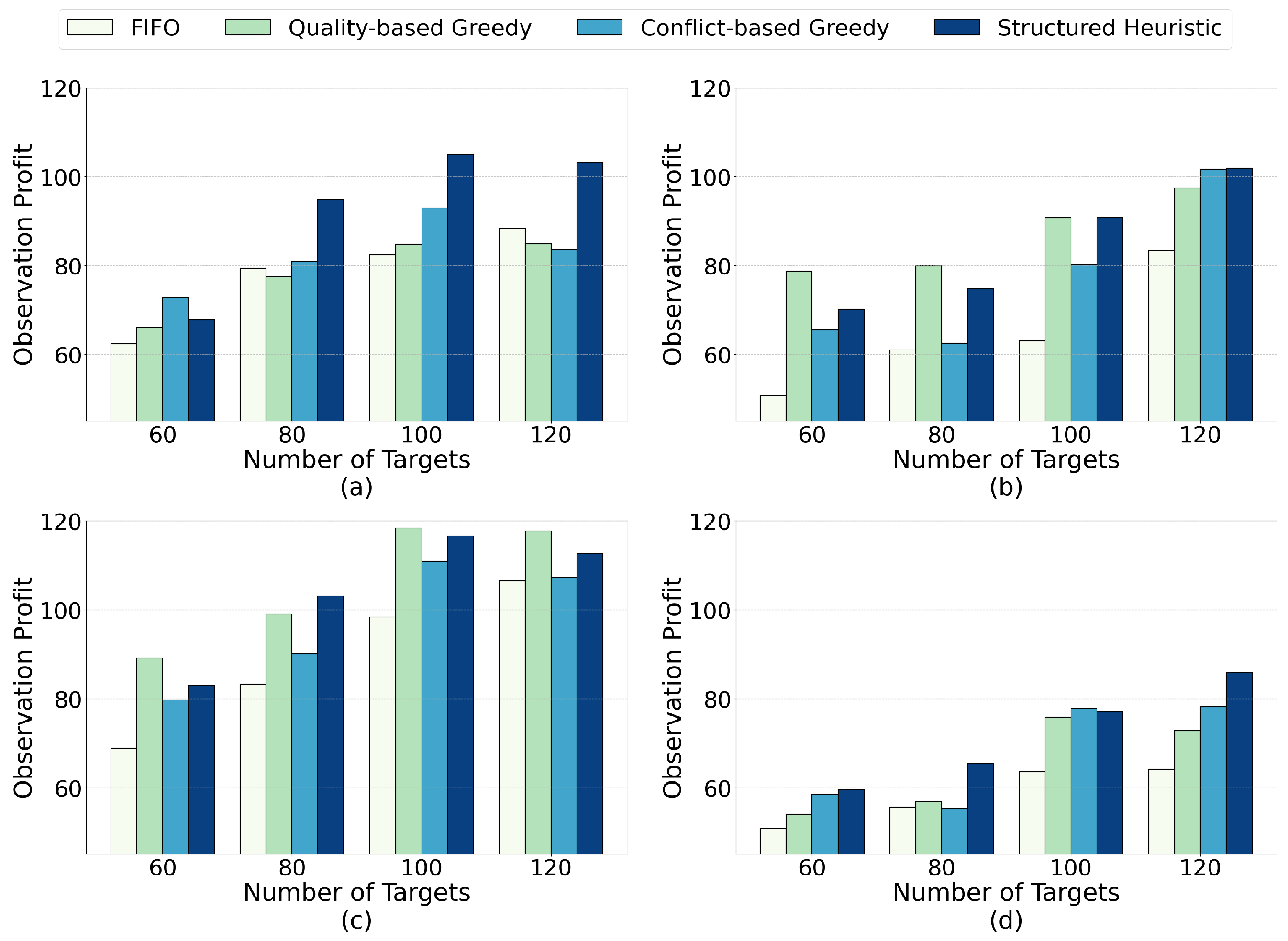
Performance is measured in terms of observation profit, defined by target priority and image quality. Results comparing the four algorithms introduced in Section 4.2 are shown in Figure 3. Figure 3a and Figure 3b correspond to 3 h and 9 h STHs, respectively, under LEO configuration (1), while Figure 3c and Figure 3d depict the 3 h STH case with LEO configurations (2) and (3), respectively. Overall, the FIFO algorithm delivers the lowest performance, as it simply maximizes the number of observed targets without accounting for priority or image quality, often selecting observations at the beginning of each VTW, where image quality is poorest. The quality-based greedy algorithm achieves the highest profit in scenarios with fewer conflicts and greater flexibility, either due to more satellites per orbit (Figure 3c) or because the STH is longer (Figure 3b), yielding up to a 35.5% improvement. However, the latter case may present practical drawbacks, as more time elapses between target identification and HR observation, which can reduce the relevance of the acquired data. The conflict-based greedy algorithm shows inconsistent performance, as not all conflicts have the same impact on scheduling, while the structured heuristic algorithm is the most robust, combining multiple heuristic indicators and balancing trade-offs to yield up to a 21.5% increase in observation profit in challenging scheduling scenarios.

By analyzing the results, we also observe significant variability in the storage time of scheduling instructions, denoted by ${\tau }_{m,s}^{\left(store\right)}$, which represents the delay between their generation and transmission to the corresponding AEOS, caused by the temporary unavailability of CTWs. In the evaluated cases, this delay ranges from 0 s, when the corresponding AEOS is immediately within the communication range, to approximately approximately 2.64 h. Since such latency may be critical in applications requiring rapid response, future work may focus on optimizing the constellation design to mitigate this effect, as well as extending the problem formulation to a multi-objective framework that explicitly incorporates observation timeliness into the solution process.

6. Conclusions

In this work, we propose an autonomous EO constellation design for intelligent target scheduling, comprising EOSs deployed at MEO and LEO. MEO EOs acquire and process LR imagery to detect targets onboard, and subsequently schedule their HR observation by LEO AEOSs. To this end, we address the AEOSSP under this setting, explicitly incorporating inter-layer communication constraints into the optimization problem and defining the observation profit in terms of target priority and image quality. We introduce several heuristic strategies to efficiently solve the problem. Among them, the quality-based greedy algorithm performs best in scenarios with few conflicts, while the structured heuristic algorithm is the most robust, delivering superior results in challenging schedules. Future work will explore ML and distributed approaches to enhance performance and scalability, as well as a multi-objective AEOSSP formulation that accounts for observation timeliness.

References

1. Leyva-Mayorga, I.; Martinez-Gost, M.; Moretti, M.; Pérez-Neira, A.; Vázquez, M.Á.; Popovski, P.; Soret, B. Satellite edge computing for real-time and very-high resolution earth observation. IEEE Trans. Commun. 2023, 71, 6180–6194. [Google Scholar] [CrossRef]
2. Wang, X.; Wu, G.; Xing, L.; Pedrycz, W. Agile Earth Observation Satellite Scheduling Over 20 Years: Formulations, Methods, and Future Directions. IEEE Syst. J. 2021, 15, 3881–3892. [Google Scholar] [CrossRef]
3. Leyva-Mayorga, I.; Soret, B.; Matthiesen, B.; Röper, M.; Wübben, D.; Dekorsy, A.; Popovski, P. Non-geostationary orbit constellation design for global connectivity. In Non-Geostationary Satellite Communications Systems; Lagunas, E., Chatzinotas, S., An, K., Beidas, B.F., Eds.; Institution of Engineering and Technology: Stevenage, UK, 2022; pp. 237–267. [Google Scholar]
4. Wang, X.; Wu, J.; Shi, Z.; Zhao, F.; Jin, Z. Deep reinforcement learning-based autonomous mission planning method for high and low orbit multiple agile Earth observing satellites. Adv. Space Res. 2022, 70, 3478–3493. [Google Scholar] [CrossRef]
5. Lemaître, M.; Verfaillie, G.; Jouhaud, F.; Lachiver, J.M.; Bataille, N. Selecting and scheduling observations of agile satellites. Aerosp. Sci. Technol. 2002, 6, 367–381. [Google Scholar] [CrossRef]
6. Xu, R.; Chen, H.; Liang, X.; Wang, H. Priority-based constructive algorithms for scheduling agile earth observation satellites with total priority maximization. Expert Syst. Appl. 2016, 51, 195–206. [Google Scholar] [CrossRef]
7. Chen, X.; Reinelt, G.; Dai, G.; Wang, M. Priority-based and conflict-avoidance heuristics for multi-satellite scheduling. Appl. Soft Comput. 2018, 69, 177–191. [Google Scholar] [CrossRef]
8. Chu, X.; Chen, Y.; Tan, Y. An anytime branch and bound algorithm for agile earth observation satellite onboard scheduling. Adv. Space Res. 2017, 60, 2077–2090. [Google Scholar] [CrossRef]
9. Long, Y.; Shan, C.; Shang, W.; Li, J.; Wang, Y. Deep Reinforcement Learning-Based Approach With Varying-Scale Generalization for the Earth Observation Satellite Scheduling Problem Considering Resource Consumptions and Supplements. IEEE Trans. Aerosp. Electron. Syst. 2024, 60, 2572–2585. [Google Scholar] [CrossRef]
10. Liu, X.; Laporte, G.; Chen, Y.; He, R. An adaptive large neighborhood search metaheuristic for agile satellite scheduling with time-dependent transition time. Comput. Oper. Res. 2017, 86, 41–53. [Google Scholar] [CrossRef]
11. Yi, W.; Wang, Y.; Zeng, Y.; Wang, Y.; Xu, J. Comprehensive Evaluation of the GF-4 Satellite Image Quality from 2015 to 2020. ISPRS Int. J. Geo-Inf. 2021, 10, 406. [Google Scholar] [CrossRef]
12. Choi, C.-S.; Baccelli, F. A Novel Analytical Model for LEO and MEO Satellite Networks based on Cox Point Processes. arXiv 2024, arXiv:2212.03549. [Google Scholar] [CrossRef]
Figure 1. Observation capability of an AEOS and a conventional EOS.
Engproc 133 00129 g001
Figure 2. Task sequence of the proposed framework. An MEO EOS m captures an LR image at τ m ( c a p ) , processes it for τ m ( p r o c ) seconds, and identifies a set of targets T m . It then generates an observation schedule for a set S of LEO AEOSs. The schedule is stored for τ m , s ( s t o r e ) seconds before being transmitted to each AEOS s, which perform the HR observation of the corresponding scheduled targets.
Engproc 133 00129 g002
Figure 3. Performance of the heuristic methods across different scenarios: (a) 3 h STH with LEO configuration (1); (b) 9 h STH with LEO configuration (1); (c) 3 h STH with LEO configuration (2); (d) 3h STH with LEO configuration (3).
Engproc 133 00129 g003
Disclaimer/Publisher’s Note: The statements, opinions and data contained in all publications are solely those of the individual author(s) and contributor(s) and not of MDPI and/or the editor(s). MDPI and/or the editor(s) disclaim responsibility for any injury to people or property resulting from any ideas, methods, instructions or products referred to in the content.