Proceeding Paper

Estimation of Gravity Gradients Using Deep Learning for Efficient Positioning with a Quantum Sensor †
1
Department of Electronics and Electrical Engineering, University of Liverpool, Liverpool L69 3GJ, UK
2
Raytheon UK, Glenrothes KY7 5PY, UK
*
Author to whom correspondence should be addressed.
Presented at the European Navigation Conference 2025 (ENC 2025), Wrocław, Poland, 21–23 May 2025.
Eng. Proc. 2026, 126(1), 22; https://doi.org/10.3390/engproc2026126022
Published: 24 February 2026
(This article belongs to the Proceedings of European Navigation Conference 2025)

Abstract

Quantum cold-atom sensors provide precise measurements of gravitational acceleration and gravity gradients. By matching these measurements to a high-resolution gravity database, a moving platform can derive its position using map-matching techniques that fuse gradient observations with inertial navigation. One such fusion technique, particle filters, is dominated by the cost of evaluating gravity gradients via surface integrals at each location. To overcome this overhead, we introduce a deep-learning model that predicts the vertical gravity gradient from a compact subset of local gravity anomaly samples, eliminating the need for full integral computations. We integrate this deep neural network into the map-matching framework, benchmark its accuracy against conventional methods, and demonstrate its real-time performance within a simulated inertial navigation system driven by a quantum sensor model.

1. Introduction

Gravity is not uniform across the Earth; it varies subtly from point to point due to the internal structure of the Earth and its uneven distribution of mass [1]. This non-uniformity can be exploited to derive the position of a moving platform using gravity gradient map-matching with classical gravimeters [2,3,4], and also cold-atom gravimeters using particle filters [5]. By map-matching the observed gravity gradients from the sensor to a gravity map, a moving platform can determine its position and use this position to correct the drift of its inertial navigation system (INS), leading to a robust navigation solution, which is immune to jamming [5].
Conventional inertial sensors operate using standard classical physics. An accelerometer measures the specific force on a proof mass as the sensor undergoes accelerations. A gyroscope can measure a rate of rotation. In both cases, one of the significant contributions to the measurement error is subtle differences in the physical parameters from sensor to sensor, which can change over time. For example, the proof mass varies from device to device. The mass is typically attached to a spring, with a spring constant that varies from device to device, it varies over time as it ages, and it changes with different environmental conditions (temperature). These slight variations in physical devices lead to biases in sensor measurements. Biases in inertial sensors lead to significant drift in INS relying on ‘dead reckoning’.
The emergence of quantum inertial sensors, based on the manipulation of cold atoms, has several potential benefits [6]. Principally, these are the potential removal of bias errors and the ability to perform extremely accurate measurements. In these systems, a small cloud of atoms of a chemical isotope is prepared in a vacuum and held in an electromagnetic trap. The kinetic energy of the confined atoms is reduced using a number of different cooling techniques [7], which makes the cloud stable (relatively speaking). The motion of the atoms within the cooled cloud is governed by quantum mechanics, which allows the individual atoms to be placed in superpositions of motional states. This means that, when subject to inertial forces, each atom can follow two distinct trajectories within the vacuum chamber and, when recombined, a measurement will show an interference pattern due to the different paths followed by each atom in the cloud. The ability to create such interference patterns is important because the phase of the interference can be configured to encode the inertial quantities of interest. Examples of such sensors are quantum gravimeters [8], quantum gradiometers [9,10], quantum accelerometers [7] and quantum gyroscopes [7]. Their importance is that they can remove biases from the sensor measurement because every atom of the same isotope is identical. The mass of each atom is known to a very high precision, and it does not change over time or in response to environmental conditions. In addition, the nature of the measurements means that the accuracy of the measurements of the inertial quantities can be orders of magnitude better than conventional classical sensors. Whilst the removal of sensor biases is an important aspect of cold-atom sensors, it is the potential for extremely accurate measurements of gravity and acceleration that is of chief importance for this paper—the use of high-precision gravity gradient measurements for position fixing and the correction of inertial drift.
Cold-atom sensors do have drawbacks. Generating interference patterns means that the motion of the atoms needs to be relatively large. This size requirement means that the sensors are large and have low measurement frequencies. At the current state of development, the cost of cold atom sensors is relatively high, which limits widespread deployment. However, as the technology matures and improves, the adoption of these sensors should grow. Despite this, the current generation of technology can be of use in positioning and navigation, and sensor-specific particle filter algorithms have been developed for map-matching and position fixing [5].
Despite its potential, implementing gravity gradient map-matching with particle filters in practice poses significant computational challenges. Particle filters require the proposal of multiple candidate solutions, which are evaluated at every update. This requires the computation of a local gravity gradient for each particle, which requires a surface integral to be computed over the area surrounding the point of interest [11].
To overcome this computational challenge, our work leverages a deep learning approach that approximates the calculation, reducing the time to compute. Instead of processing the entire set of points needed for a complete integral calculation, the network operates on a subset of representative points. This method bypasses the integral for each proposed position in the particle filter. By training the network to learn the mapping from these selected input points to the gravity gradient, we can perform efficient predictions that maintain high accuracy in real-time map-matching.
The remainder of this paper is organised as follows. In Section 2, we review the background literature and introduce the concepts of inertial drift, map-matching, and both classical and quantum sensing approaches. Section 3 details the materials and methods, with a particular focus on our deep neural network architecture, the data preparation process, and the training procedures. In Section 4, we present a quantitative analysis comparing the performance of our deep learning approach against conventional computational methods, while Section 5 concludes with a discussion of the key findings and potential directions for future research.

2. Background

Position fixing is vital in many sectors, as it allows safe and efficient navigation. Obtaining a position fix presents significant challenges due to several factors. Global navigation satellite systems (GNSS) are vulnerable to jamming. Furthermore, alternative terrestrial systems, like Loran and eLoran, lack the necessary infrastructure to be utilised as a robust backup. Pure inertial navigation systems, although immune to jamming and spoofing, have an inherent instability due to sensor drift over time [12].
To compensate for the instability of INS, map-matching techniques can be used. These methods correlate measurements or derived states with features represented in a digital map database to provide periodic position corrections or bounds on the estimated INS position. For example, Terrain Referenced Navigation (TRN), often utilised in defence, compares measurements of the underlying terrain (such as altitude profiles obtained from radar altimeters) against a digital elevation model to derive a position fix [13]. An emerging technique is gravitational map-matching, which seeks to correlate measurements of local gravity field variations with a high-resolution gravity map, offering a potential jam-resistant navigation solution [2,3,5,14,15,16,17].

2.1. Prior Work on Gravity Map-Matching

Gravity map-matching can be utilised as a means to enhance inertial navigation by correcting drift errors. Studies have used classical gravimeters to capture local gravity variations and match them against a gravity database [4]. This initial research demonstrated that even subtle gravity variations can reduce the errors experienced in inertial navigation systems.
Probabilistic methods, such as particle filters, have been used to manage the uncertainties resulting from sensor measurements. Particle filters maintain a set of candidate position estimates and continuously refine the navigation solution as measurements are taken [5].
While work on gravity map-matching has been demonstrated to improve the performance of inertial navigation systems, it is computationally expensive. This motivates research into more efficient and advanced methods, such as deep learning, to enable real-time and robust gravity map-matching-based navigation solutions.

2.2. Deep Learning in Gravimetry

Accurate modelling of Earth’s gravitational features plays a pivotal role in gravity map-matching. In recent years, machine learning and deep learning techniques have become increasingly relevant for tackling data gaps, fusing data sources, and also increasing their resolution by leveraging large datasets and complex neural network architectures.
A 2024 study demonstrated that machine learning models (like random forests, support vector machines, and neural networks) achieve significantly higher accuracy in predicting gravity anomalies over data-sparse regions when compared with Kriging interpolation [18]. These enhanced gravity anomaly predictions could lead to more reliable position fixes when using gravity map-matching. One challenge with gravity-aided inertial navigation is addressing the computational intensity with traditional algorithms such as particle filters. Deep learning allows neural networks to be used as a pattern matcher for gravity data, attempting to compare measured gravity gradient patterns to a stored map [19]. The results indicate that a neural network yields faster and more robust position solutions, performing the map-matching calculations in one forward pass [19].

2.3. Quantum Cold-Atom Interferometry

Quantum cold-atom interferometry sensors exploit the wave nature of atoms to perform precision inertial measurements [6]. Laser pulses are used to split, redirect, and recombine matter-waves of ultracold atoms. As these atoms fall freely, they accumulate a phase shift proportional to the experienced acceleration; once recombined, the phase of the interference fringe reveals the acceleration [9]. Atom interferometric sensors measure gravity absolutely, meaning that these quantum gravimeters exhibit virtually zero long-term drift, unlike spring or quartz gravimeters that must be regularly calibrated [5].
A quantum gravity gradiometer uses two separate atomic clouds [10]. By using the same laser for both clouds, gravity gradients can be measured, as the differential phase between the upper and lower interferometers is directly proportional to the local gravity gradient, ignoring common-mode accelerations [9].

3. Materials and Methods

3.1. Deep Learning Architecture

We developed a deep neural network (DNN) approach to estimate the vertical gravity gradient from gravity anomaly data. The network was implemented using the PyTorch 2.6 deep learning framework [20] and was optimised with the Optuna hyperparameter optimisation library [21]. It ingests a 10,000-dimensional vector of local gravity anomaly measurements and outputs a vertical gravity gradient. The Optuna search space included the number of hidden layers, neurons per layer, learning rate, optimiser choice, learning rate scheduler, dropout rate, and early stopping patience. The data used for training covered a 10,000 km2 region between Liverpool and York, derived from the SRTM2 gravity dataset [22]. The SRTM2 gravity dataset provides terrain-corrected gravity anomalies. The anomalies were sampled on a regular grid, and gravity values at the locations on the polar grid (Figure 1) were obtained using linear interpolation.
Based on the Optuna results, the final model comprises six fully connected hidden layers, each with 512 neurons, and Rectified Linear Unit (ReLU) activations after each layer. To stabilise training, a small dropout rate of 0.000647 was used. The network was trained with the Adam optimiser at an initial learning rate of 7.1106 × 10⁻⁴ and a batch size of 512, with learning rate decay governed by a CosineAnnealingLR scheduler. Early stopping with a patience of four epochs on the validation loss was employed to prevent overfitting.

3.2. Data Preparation

The vertical gravity gradient represents the rate of change in gravity with height, usually expressed as g H , where H is the height above the geoid. Section 2.20 of [11] derives formulas for this quantity by splitting it into two parts: a normal component γ H (the gradient in a theoretical normal gravity field) and an anomalous component Δ g H (due to local gravity anomalies).
g H = γ H + Δ g H
Here, Δ g denotes the gravity anomaly at point P, defined as the difference between the observed gravity reduced to the reference ellipsoid and the normal gravity on the ellipsoid. This is the classical Helmert gravity anomaly [11].

3.2.1. Normal Gravity Gradient

The normal gravity gradient γ H is the vertical gravity gradient calculated using the WGS84 ellipsoid Earth model [23]. Equations (2–147) and (2–148) from [11] can be used to compute this value, which stems from applying Bruns’ formula to the ellipsoidal normal field:
γ H = 2 γ J 2 ω 2 ,
where J is the mean curvature of the level ellipsoid at point P and ω is Earth’s angular rotation speed. The second term 2 ω 2 is significantly smaller, but its effects accumulate and become noticeable over longer time periods.

3.2.2. Anomalous Vertical Gradient

The anomalous component Δ g H is the contribution to the vertical gravity gradient from local gravity anomalies; these can be caused by uneven mass distribution within the Earth. The vertical gravity gradient at a point P (denoted ( Δ g H ) P ) is an integral over the surrounding gravity anomaly field. In local polar coordinates ( s , α ) (with s = horizontal distance from P, and α = the azimuth angle around P), the formula is:
Δ g H P = 1 2 π 0 2 π 0 s 0 Δ g ( s , α ) Δ g P s 3 s   d s d α ,
where Δ g ( s , α ) is the gravity anomaly at a neighbouring point Q located distance s from P in direction α , and Δ g P is the anomaly at P. The integration covers a circular disk of radius s 0 around point P. Essentially, this formula computes the vertical gradient (rate of change with height) of the gravity anomaly at P by averaging the anomaly differences in a neighbourhood of P, weighted inversely by distance squared. We approximate it by a double summation over a discrete polar grid on the local tangent plane around P.
We divide the disk of radius s 0 into concentric rings (radial segments) and angular sectors, sample the gravity anomaly at each small area element, and sum up the contributions; the double integral becomes a double summation:
Δ g H P = 1 2 π i = 1 N j = 0 M 1 Δ g ( s i , α j ) Δ g P s i 3 s i   Δ s Δ α ,
where s i = i , Δ s is the radial distance for the ith ring (see below on why the sum starts at i = 1 ), and α j = j , Δ α is the azimuth of the centre of the jth sector. Each term in this summation corresponds to the integrand evaluated at the centre of a small area. Whilst it is possible to pre-calculate these values for a given altitude, the variation in the gradient with altitude means that these values would require very large look-up tables unless they are calculated point-by-point. Although the formulation is expressed in polar coordinates, all gravity anomalies were sampled from a regular grid and evaluated using linear interpolation.
By following this approach, we are able to compute an estimate for the vertical gravity gradient at any point P by essentially performing a weighted average of the surrounding gravity anomalies in a polar layout. The anomaly values are originally stored on a rectangular grid provided by SRTM2 gravity. The polar grid shown in Figure 1, and referenced in Equation (4), is used only for evaluating the anomaly at point P. The values on this polar grid are obtained by interpolating the polar points from the rectangular grid.
To produce the dataset required for the neural network, the study area is divided into discrete geographic chunks, where the gravity gradient for each cell is stored in an array, along with the set of gravity anomaly Δ g .
The training dataset covered a region of approximately 10,000 km2, extending from 53.2° N to 54.0° N and from 3.4° W to 1.6° W, between Liverpool, Preston, and York, sampled at a ~100 m grid resolution in both north–south and east–west directions. Each grid cell contained 10,000 local gravity anomaly values as input features and one corresponding vertical gravity gradient value as the output target. The gravity disturbances were obtained from the SRTM2 gravity dataset [22], with intermediate values estimated by linear interpolation. Data were generated at five discrete altitudes (0 m, 250 m, 500 m, 750 m, and 1000 m) to capture height-dependent variations.

3.3. Training Procedure

Prior to training, both inputs and outputs were scaled using feature-wise standardisation based on statistics computed from the training dataset. Thus, all reported losses are expressed relative to this scaled dataset. After loading the dataset into memory (with a 90/10 training/validation split), we launched an Optuna study over 250 trials; the hyperparameter search space is defined in Table 1.
During each trial we recorded training and validation losses as well as the instantaneous learning rate. Optuna’s pruning mechanism halted underperforming trials, improving efficiency. Once the study was completed, the best hyperparameters were used to re-initialise and retrain a model on the full training split with early stopping (patience = 4), and the final weights were saved for reproducibility.
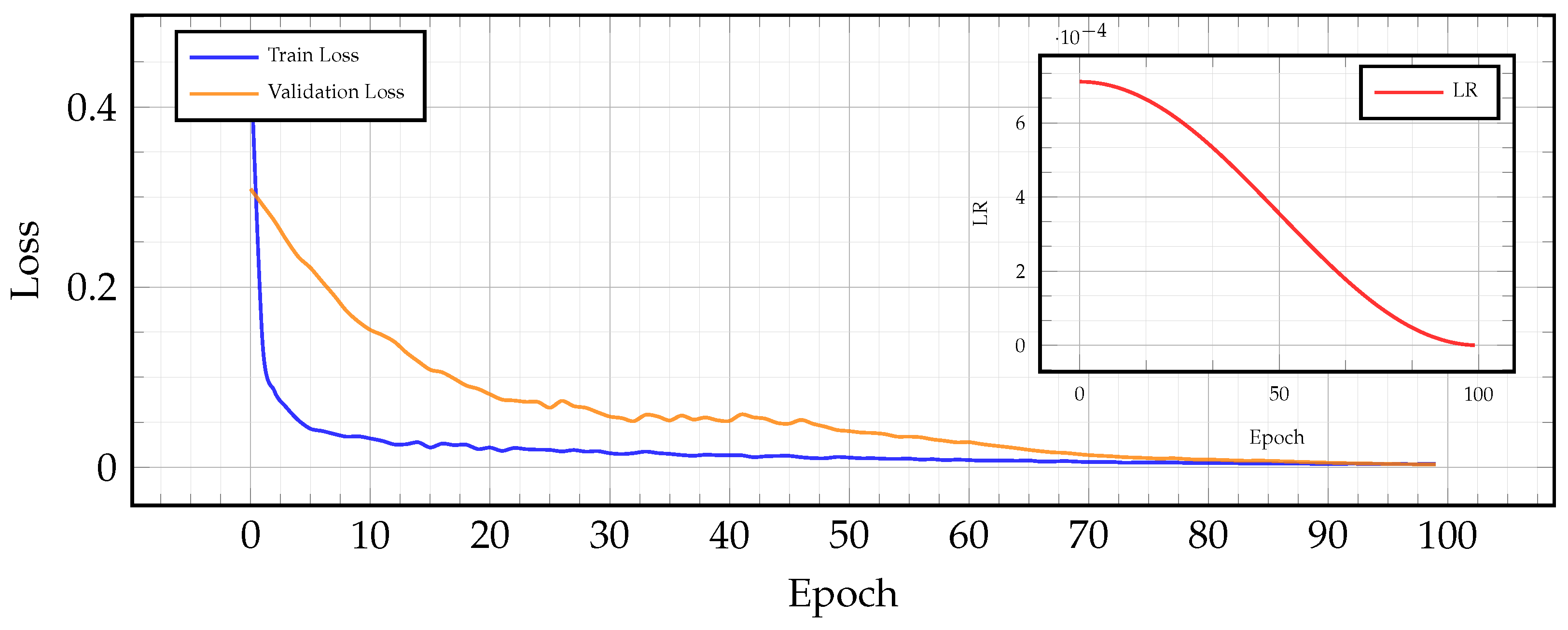
Figure 2 (optimal hyperparameters in Table 1) shows the training loss (blue) plunging in the first ten epochs, with the validation loss (orange) following a steadier but uninterrupted decline. After epoch 10 both curves descend smoothly toward zero and converge by epoch 60, indicating minimal overfitting. The inset reveals the CosineAnnealingLR’s gradual learning-rate decay, which underpins this stable convergence.

4. Results

4.1. Model Performance

To assess the model’s performance, we evaluated final metrics of training and validation loss computed using the root mean squared error (RMSE) loss function, obtained after early stopping. At convergence, the model achieved low training and validation losses, indicating highly accurate predictions of vertical gravity gradients, as shown in Table 2. The validation loss demonstrates minimal difference relative to the training loss, confirming effective generalisation without significant overfitting.
These loss values confirm the effectiveness of the chosen hyperparameters (Table 1) and optimisation procedures, particularly highlighting the contribution of the smooth learning rate schedule provided by the CosineAnnealingLR scheduler (Figure 2).

4.2. Quantitative Comparison with Baseline Methods

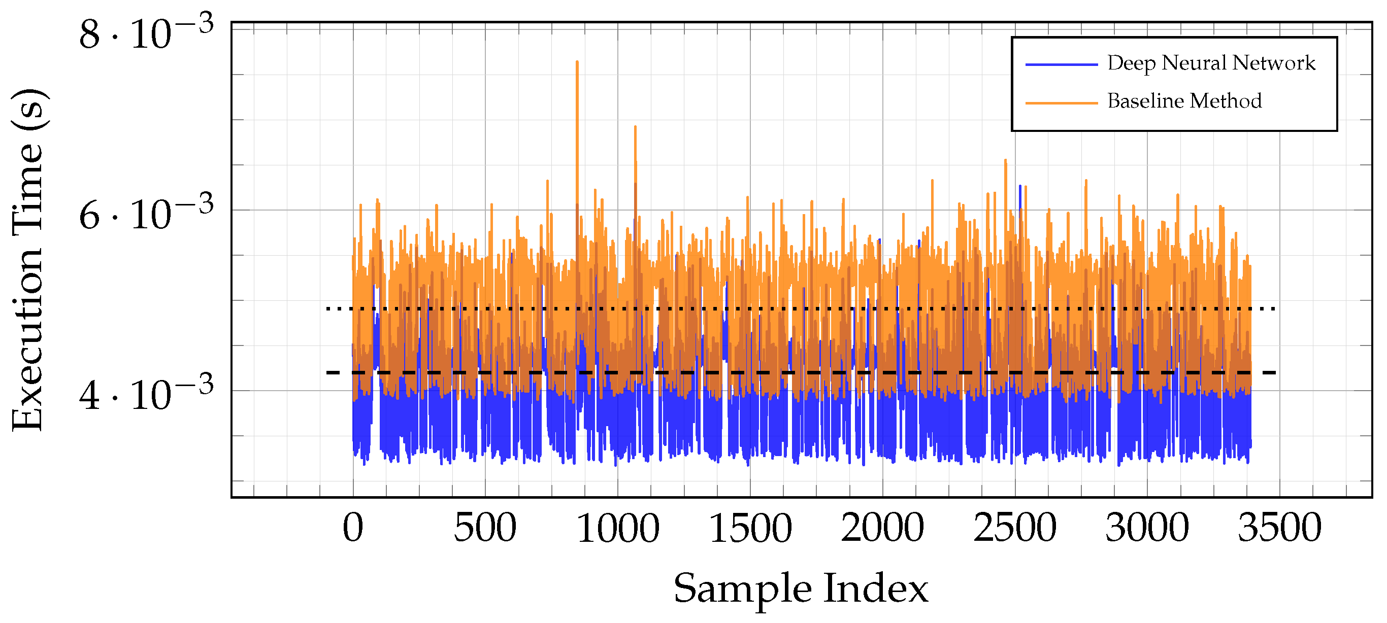
To evaluate both the computational efficiency and the accuracy of our DNN-based gravity-gradient estimator, we compared it against the conventional surface-integral computation over 3500 test points, shown in Figure 3. All tests were run using Python 3.11.5 on Debian 12 on a workstation equipped with an AMD Ryzen 9 3900X CPU and an NVIDIA RTX 4070 GPU with PyTorch 2.4.1, CUDA 12.4 and cuDNN 9.
Figure 3 shows the per sample execution times for the deep neural network (blue) and the baseline method (orange). The deep neural network requires, on average, 4.2 × 10⁻³ s per inference, which is approximately 14.37% faster than the baseline’s mean of 4.91 × 10⁻³ s. Moreover, the DNN’s inference times exhibit markedly lower variance, leading to more predictable real-time performance. This reduction in both mean latency and jitter aids in solving the primary bottleneck in a particle filter-based map-matching loop, where many gradient evaluations must be carried out at each update.
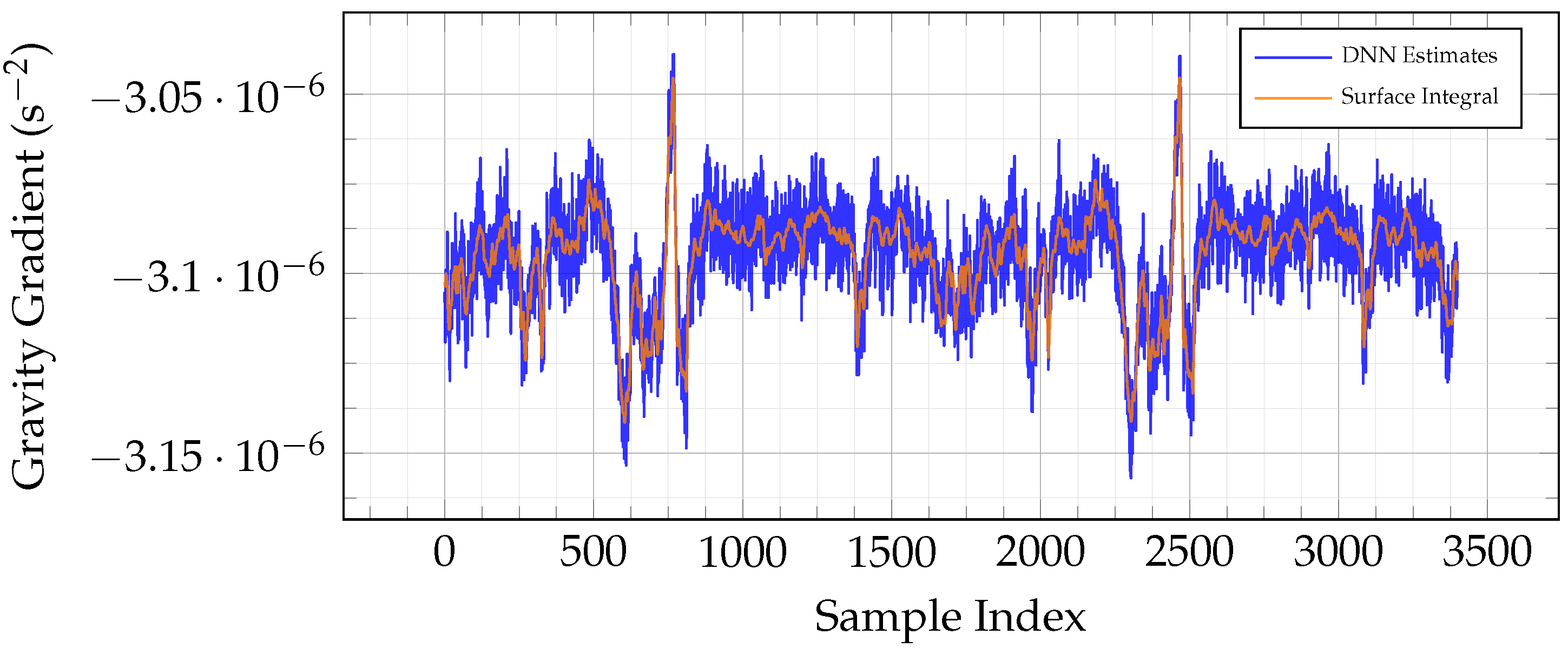
In Figure 4, we overlay the DNN’s gravity-gradient estimates (blue) on the surface integral (orange). The root mean square error (RMSE) across all samples is under 8.02 × 10⁻⁹ s−2, which is far below the accuracy of current sensors [24].

4.3. Application to Simulated Navigation Scenario

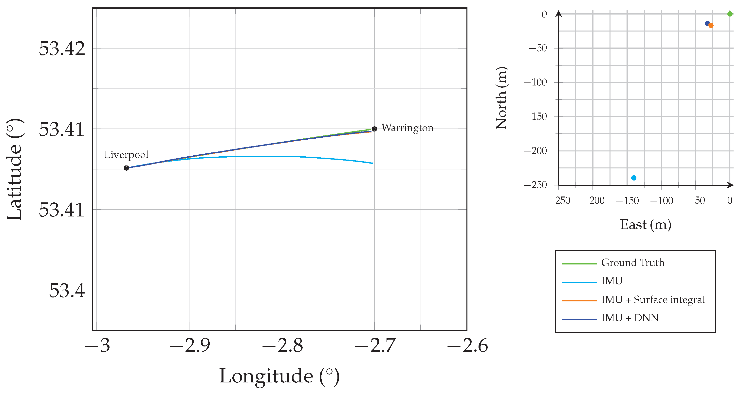
We applied the deep neural network estimator to the particle filter method described in [5]. This resulted in an error over a 22.5 km 360-s trial of 35.5 m; the conventional method had an error of 32.3 m, while a conventional aviation IMU achieved an error of 277.6 m.

5. Conclusions

In this work, we have demonstrated that a deep neural network can approximate the vertical gravity gradient efficiently, a computation that traditionally relies on an expensive surface-integral evaluation. By training a six-layer fully connected network on local gravity anomaly samples, we achieve a computation time of 4.20 × 10⁻³ s per point—approximately 14.37% faster than the classical method—while maintaining an RMSE of just 8.02 × 10⁻⁹ s−2.
When integrated into a simulated inertial navigation scenario with a cold-atom sensor model, the neural-network estimator marked an improvement in computation time for the navigation algorithm, while maintaining an error of 35.5 m in a simulated trial for an airborne sensor displayed in Figure 5.
In summary, by replacing the heavy numerical integration with a single forward pass through a deep neural network, we have demonstrated that a machine learning surrogate can be used as part of an integrated inertial–gravity map-matching algorithm. This use of machine learning has the potential to reduce the computational load associated with positioning using map-matching with gravity gradients. The proof of principle presented here can be improved upon, and this will guide our future work.

Author Contributions

Conceptualisation, J.F.R., M.W., and D.J.C.; methodology, D.J.C.; software, D.J.C., and M.W.; validation, D.J.C.; formal analysis, D.J.C.; investigation, D.J.C.; resources, D.J.C.; data curation, D.J.C.; writing—original draft preparation, D.J.C., and J.F.R.; writing—review and editing, D.J.C., J.F.R., M.W., K.M., and G.M.; visualisation, D.J.C.; supervision, J.F.R., K.M., and G.M.; project administration, D.J.C. All authors have read and agreed to the published version of the manuscript.

Funding

This research received no external funding.

Institutional Review Board Statement

Not applicable.

Informed Consent Statement

Not applicable.

Data Availability Statement

The datasets generated and analysed during the current study are available from the corresponding author upon reasonable request.

Conflicts of Interest

Author Grant MacLean was employed by the company Raytheon. The remaining authors declare that the research was conducted in the absence of any commercial or financial relationships that could be construed as a potential conflict of interest.

References

  1. Bouman, J.; Ebbing, J.; Fuchs, M.; Sebera, J.; Lieb, V.; Szwillus, W.; Haagmans, R.; Novák, P. Satellite gravity gradient grids for geophysics. Sci. Rep. 2016, 6, 21050. [Google Scholar] [CrossRef] [PubMed]
  2. Wang, H.; Wu, Y.; Wu, Y.; Zhou, X. Gravity matching navigation algorithm based on iterated closest contour point. IET Radar Sonar Navig. 2016, 10, 862–867. [Google Scholar] [CrossRef]
  3. Wang, H.; Wu, Y.; Wu, Y.; Zhou, X. Application of gravity matching algorithm based on iterated closest contour point. Sensors 2017, 17, 1851. [Google Scholar]
  4. DeGregoria, A. Gravity Gradiometry and Map Matching: An Aid to Aircraft Inertial Navigation Systems. Master’s Thesis, Air Force Institute of Technology, Wright-Patterson AFB, Graduate School of Engineering and Management, Dayton, OH, USA, 2010. [Google Scholar]
  5. Phillips, A.M.; Wright, M.J.; Riou, I.; Maddox, S.; Maskell, S.; Ralph, J.F. Position fixing with cold atom gravity gradiometers. AVS Quantum Sci. 2022, 4, 024404. [Google Scholar] [CrossRef]
  6. Wright, M.J.; Anastassiou, L.; Mishra, C.; Davies, J.M.; Phillips, A.M.; Maskell, S.; Ralph, J.F. Cold atom inertial sensors for navigation applications. Front. Phys. 2022, 10, 994459. [Google Scholar] [CrossRef]
  7. Geiger, R.; Landragin, A.; Merlet, S.; Pereira Dos Santos, F. High-accuracy inertial measurements with cold-atom sensors. AVS Quantum Sci. 2020, 2, 024702. [Google Scholar] [CrossRef]
  8. Janvier, C.; Ménoret, V.; Desruelle, B.; Merlet, S.; Landragin, A.; Pereira dos Santos, F. Compact differential gravimeter at the quantum projection-noise limit. Phys. Rev. A 2022, 105, 022801. [Google Scholar] [CrossRef]
  9. Yu, N.; Thompson, R.J.; Kellogg, J.R.; Aveline, D.C.; Maleki, L.; Kohel, J.M. A Transportable Gravity Gradiometer Based on Atom Interferometry; NASA Tech Brief NPO-46280; Jet Propulsion Laboratory, California Institute of Technology: Pasadena, CA, USA, 2010. [Google Scholar]
  10. McGuirk, J.M.; Foster, G.T.; Fixler, J.B.; Snadden, M.J.; Kasevich, M.A. Sensitive absolute-gravity gradiometry using atom interferometry. Phys. Rev. A 2002, 65, 033608. [Google Scholar] [CrossRef]
  11. Hofmann-Wellenhof, B.; Moritz, H. Physical Geodesy, 2nd, corrected ed.; Springer: Vienna, Austria; New York, NY, USA, 2006; Revised edition of the 1st ed. (2005). [Google Scholar] [CrossRef]
  12. Groves, P.D. Principles of GNSS, Inertial, and Multi-Sensor Integrated Navigation Systems; GNSS Technology and Applications Series; Artech House: Boston, MA, USA, 2007. [Google Scholar]
  13. Ma, T.; Ding, S.; Li, Y.; Fan, J. A review of terrain aided navigation for underwater vehicles. Ocean Eng. 2023, 281, 114779. [Google Scholar] [CrossRef]
  14. Affleck, C.; Jircitano, A. Passive Gravity Gradiometer Navigation System. In IEEE Position Location and Navigation Symposium (PLANS); IEEE: New York, NY, USA, 1990; pp. 60–66. [Google Scholar] [CrossRef]
  15. Kamgar-Parsi, B.; Kamgar-Parsi, B. Vehicle Localization on Gravity Maps. In Proceedings Volume 3693, Unmanned Ground Vehicle Technology; SPIE: Bellingham, WA, USA, 1999; pp. 182–191. [Google Scholar] [CrossRef]
  16. Jekeli, C. Precision Free-Inertial Navigation with Gravity Compensation by an Onboard Gradiometer. J. Guid. Control. Dyn. 2006, 29, 704–713. [Google Scholar] [CrossRef]
  17. Wu, L.; Wang, H.; Chai, H.; Hsu, H.; Wang, Y. Research on Relative Positions-Constrained Pattern Matching Method for Underwater Gravity-Aided Inertial Navigation. J. Navig. 2015, 68, 937–950. [Google Scholar] [CrossRef]
  18. Liu, Y.; Zhang, Y.; Pang, Q.; Liu, S.; Li, S.; Shi, X.; Bian, S.; Wu, Y. Gravity Predictions in Data-Missing Areas Using Machine Learning Methods. Remote Sens. 2024, 16, 4173. [Google Scholar] [CrossRef]
  19. Xiong, L.; Ma, J.; Tian, J.w. Gravity Gradient Aided Position Approach Based on EKF and NN. In Proceedings of the 2011 CSRSWTC, Harbin, China, 26–30 July 2011. [Google Scholar] [CrossRef]
  20. Paszke, A.; Gross, S.; Massa, F.; Lerer, A.; Bradbury, J.; Chanan, G.; Killeen, T.; Lin, Z.; Gimelshein, N.; Antiga, L.; et al. PyTorch: An Imperative Style, High-Performance Deep Learning Library. arXiv 2019, arXiv:1912.01703. [Google Scholar] [CrossRef]
  21. Akiba, T.; Sano, S.; Yanase, T.; Ohta, T.; Koyama, M. Optuna: A Next-generation Hyperparameter Optimization Framework. arXiv 2019, arXiv:1907.10902. [Google Scholar]
  22. Hirt, C.; Yang, M.; Kuhn, M.; Bucha, B.; Kurzmann, A.; Pail, R. SRTM2gravity: An Ultrahigh Resolution Global Model of Gravimetric Terrain Corrections. Geophys. Res. Lett. 2019, 46, 4618–4627. [Google Scholar] [CrossRef]
  23. National Imagery and Mapping Agency. Department of Defense World Geodetic System 1984: Its Definition and Relationships with Local Geodetic Systems; Technical Report TR8350.2; National Imagery and Mapping Agency (NIMA): Bethesda, MD, USA, 1997; Amendment 1 added 3 January 2000. [Google Scholar]
  24. Stray, B.; Lamb, A.; Kaushik, A.; Vovrosh, J.; Rodgers, A.; Winch, J.; Hayati, F.; Boddice, D.; Stabrawa, A.; Niggebaum, A.; et al. Quantum sensing for gravity cartography. Nature 2022, 602, 590–594. [Google Scholar] [CrossRef] [PubMed]
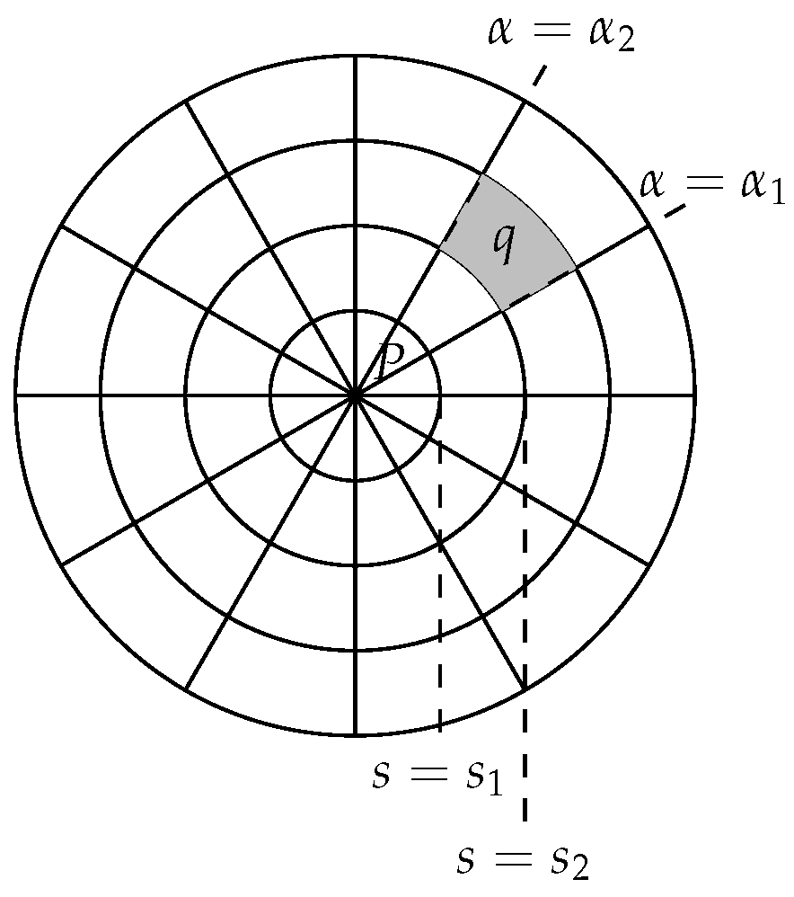
Figure 1. Partition of the local area around point P into concentric rings and angular sectors in polar coordinates.
Engproc 126 00022 g001
Figure 2. Training and validation loss across epochs with the learning rate schedule in the top right.
Engproc 126 00022 g002
Figure 3. Execution times for the deep neural network (blue) and the baseline method (orange).
Engproc 126 00022 g003
Figure 4. Surface integral values (orange) vs. neural network estimates (blue) over all samples.
Engproc 126 00022 g004
Figure 5. Trial of three different navigation solvers from Liverpool city centre to Warrington, with an inset figure displaying final position solutions.
Engproc 126 00022 g005
Table 1. Hyperparameter search space used in the optimisation process, and final model selection.
ParameterSearch SpaceTypeFinal Value
Learning ratelog-uniform on [10−6, 10−2]Continuous7.1106 × 10−4
Hidden layers3–12Integer6
Hidden features{128, 256, 512, 1024, 2048}Categorical512
Dropout rate[0.0, 0.5]Continuous6.47 × 10−4
Optimiser{Adam, AdamW, RMSprop, SGD}CategoricalAdam
Scheduler{StepLR, CosineAnnealingLR, none}CategoricalCosineAnnealingLR
Early-stopping patience3–10Integer4
StepLR specificsStep size 1–10, γ [ 0.5 , 1.0 ] Integer/continuous
Table 2. Final loss values at convergence.
MetricValue (Scaled Units)
Final training loss0.0034874
Final validation loss0.0012236
Disclaimer/Publisher’s Note: The statements, opinions and data contained in all publications are solely those of the individual author(s) and contributor(s) and not of MDPI and/or the editor(s). MDPI and/or the editor(s) disclaim responsibility for any injury to people or property resulting from any ideas, methods, instructions or products referred to in the content.