Polarimetric Space–Time Adaptive Processing in Airborne FDA Radar

Abstract

Polarimetric space–time adaptive processing (PSTAP) introduces polarization domain information alongside the space–time domain. By exploiting the differences in polarimetric scattering characteristics between targets and clutter, PSTAP significantly improves the detection performance for slow-moving targets and has become an important technology in the airborne radar community. However, the Conventional polarimetric STAP still faces the severe range ambiguity problem caused by high pulse repetition frequency (PRF) in high-speed scenarios. To overcome range ambiguity, this paper introduces the frequency diverse array (FDA) into polarimetric STAP and develops an FDA-PSTAP framework. First, we establish the fundamental signal processing procedure for FDA-PSTAP. Second, the full-dimensional (FD) FDA-PSTAP is developed according to the MVDR principle. Finally, to reduce the sample requirement for training samples, a reduced-dimensional (RD) FDA-PSTAP is proposed by designing a proper reduced-dimension transformation matrix. Numerical results demonstrate that the proposed FDA-PSTAP effectively suppresses range-ambiguous clutter. Under limited training samples, the proposed reduced-dimensional FDA-PSTAP reduces the output SINR loss by 15–17 dB compared with the full-dimensional counterpart in the main clutter region. When the number of training samples is doubled, the proposed method approaches the optimal performance with a gap of 1–2 dB across the entire Doppler spectrum, confirming its robustness and practical applicability.

1. Introduction

As a state-of-the-art signal processing solution for identifying moving targets via airborne radar platforms, space–time adaptive processing (STAP) is universally recognized as a leading algorithmic framework in this field [1,2,3,4,5]. Ever since Brennan’s groundbreaking research in 1973 [6], this adaptive processing methodology has garnered persistent interest from both academic scholars and industrial practitioners, thanks to its outstanding performance in mitigating intense ground clutter echoes and elevating the target detection sensitivity of radar systems. Conventional STAP has limited capability for detecting slow-moving targets in the main clutter region of the space-time domain. To address this limitation, reference [7] introduces polarization information into STAP and develops polarimetric STAP (PSTAP). Polarization constitutes an intrinsic attribute of electromagnetic waves. Measurement of the amplitude and phase of target returns across diverse polarization states allows the construction of its polarimetric scattering matrix, which enables the retrieval of physical attributes including geometric configuration, symmetry, alignment, and compositional material of the target. The history of radar polarimetry investigations goes back to the late 1940s, initiated by Sinclair’s introduction of the target polarimetric scattering matrix [8]. Subsequently, Park et al. [9] pioneered the polarimetric space–time generalized likelihood ratio test (GLRT) detection theory, which promoted the integration of adaptive processing in the polarization domain and the space–time domain. Evidence indicates that by exploiting the differences in polarimetric scattering properties between targets and clutter, PSTAP can markedly improve the detection performance for slow-moving targets located in the primary clutter zone of the space–time domain.

Modern airborne radar systems increasingly employ high-velocity carrier platforms because these platforms offer superior agility and rapid response capability in real-world operational scenarios. These fast-moving carriers are prone to severe Doppler aliasing artifacts, necessitating a high pulse repetition frequency (PRF) to fulfill the Nyquist sampling criterion across the Doppler dimension. Nevertheless, high PRF inherently curtails the unambiguous detection range, thereby introducing prominent range aliasing artifacts. Classical PSTAP algorithms are predominantly derived under the ideal assumption that range-ambiguous components are absent. However, once mixed ambiguous range echoes contaminate the received signals, the standard STAP architecture fails to discriminate reflected waveforms originating from different range bins, because it lacks additional range-adaptive space–time degrees of freedom. This deficiency ultimately leads to drastic degradation in the system’s clutter suppression capacity.

A host of technical approaches have been explored in prior literature to mitigate the detrimental impacts induced by range aliasing. These include multiple-PRF (staggered PRF) operation [10,11,12,13,14], elevation spatial filtering [15,16,17,18,19] and waveform diversified array [20,21,22,23,24], among others. The first category encompasses traditional non-adaptive techniques, among which multiple-PRF (staggered PRF) operation is the most widely employed. By transmitting pulses at two or more distinct PRFs and comparing the detected ranges, ambiguous returns can be resolved. However, this approach suffers from inherent limitations, including blind speeds, increased system complexity, and degraded data update rates, which restrict its applicability in modern high-performance radar systems. The remaining two categories seek to introduce extra range-associated adaptive dimensions. Spatial filtering schemes leverage vertically distributed antenna units to unlock extra adaptive dimensions in the elevation domain. Echo signals reflected from disparate range bins correspond to distinct elevation incident angles, which enables researchers to isolate aliased clutter components relying on elevation angle features. Provided that a sufficient number of antenna channels are equipped, this strategy delivers competent performance for resolving range ambiguity. Its performance, however, deteriorates sharply under insufficient array element configurations. In addition, extra vertical antennas raise the overall hardware overhead, a critical drawback for airborne radar equipment with strict load constraints. In contrast, waveform diversified arrays extract range-variant signal signatures via customized transmit signal parameters, including carrier frequency, phase offset and modulation formats. Reflected echoes from separate range gates carry unique waveform-specific features, which supply supplementary range-dependent adaptive degrees of freedom. Through tailored demodulation pipelines and subsequent signal manipulation, waveform diverse array systems eliminate range aliasing interference without imposing dramatic hardware burdens on airborne radar hardware implementations.

The frequency diverse array (FDA) radar stands as a typical prototype among all waveform-varying array radar frameworks. By imposing subtle frequency shifts between neighboring transmitting antennas, FDA radar embeds joint range-angle coupling signatures into the collected echo data, rendering it a promising candidate to tackle range aliasing issues. Over recent years, FDA technology has been deployed across numerous radar signal processing domains, including spectral parameter estimation [25,26], adaptive beamforming design [27,28], target recognition and detection [29], and unwanted interference elimination [30,31]. Even so, research efforts focusing on FDA-based PSTAP remain far less extensive relative to the above-mentioned research branches, leaving ample room for deeper exploration. It is worth noting that although reduced-dimensional FDA-STAP has been developed for range-ambiguous clutter suppression with limited training samples [31], it operates purely in the space–time domain and cannot distinguish slow-moving targets from clutter when their space–time signatures overlap in the main clutter region. It should be noted that polarimetric information provides an additional discrimination dimension based on the physical scattering differences between targets and clutter, which has been verified in [7]. Motivated by these works, this paper investigates an FDA-assisted PSTAP framework to realize robust clutter attenuation amid severe range aliasing scenarios.

To this end, this paper derives the fundamental signal model of FDA-PSTAP, including signal transmission, signal reception, frequency mixing, matched filtering and model approximation. These processing procedures differ from those of Conventional STAP. Furthermore, it is worth highlighting that the optimum FDA-PSTAP filter hinges on perfectly known clutter-plus-noise covariance matrix (CNCM) entries, a theoretical quantity that rarely exists in realistic radar operations and must be approximated using sampled echo training samples. Insufficient training sample counts [32] yield biased covariance estimates. This in turn causes substantial performance degradation in PSTAP. Even though the Reed–Mallett–Brennan (RMB) criterion offers a theoretical benchmark for the minimal snapshot quantity, this sampling threshold can hardly be satisfied in many practical operating environments. To overcome this issue, we exploit the idea of dimension reduction and develop an effective reduced-dimensional (RD) FDA-PSTAP, named RD-FDA-PSTAP. The proposed method selects a small number of transmit time and receive channels to construct a reduced-dimension transformation matrix. Then, the data dimension is reduced significantly, making it satisfy the RMB rule. Finally, the RD-FDA-PSTAP weight is formulated according to the minimum variance distortionless response. Numerical results show that the proposed signal model of FDA-PSTAP can effectively reject range-ambiguous clutter, and the developed RD-FDA-PSTAP method achieves effective performance under limited training samples.

Notation: In this paper, ${\mathbf{I}}_M$ denotes the identity matrix of size $M$. The symbol $\otimes$ refers to the Kronecker product. For a matrix or vector, ${(\cdot )}^T$ and ${(\cdot )}^H$ are used to represent the transpose and Hermitian transpose, respectively. The complex field is denoted by $ℂ$, while $\mathbb{E}(\cdot )$ denotes mathematical expectation.

2. Background

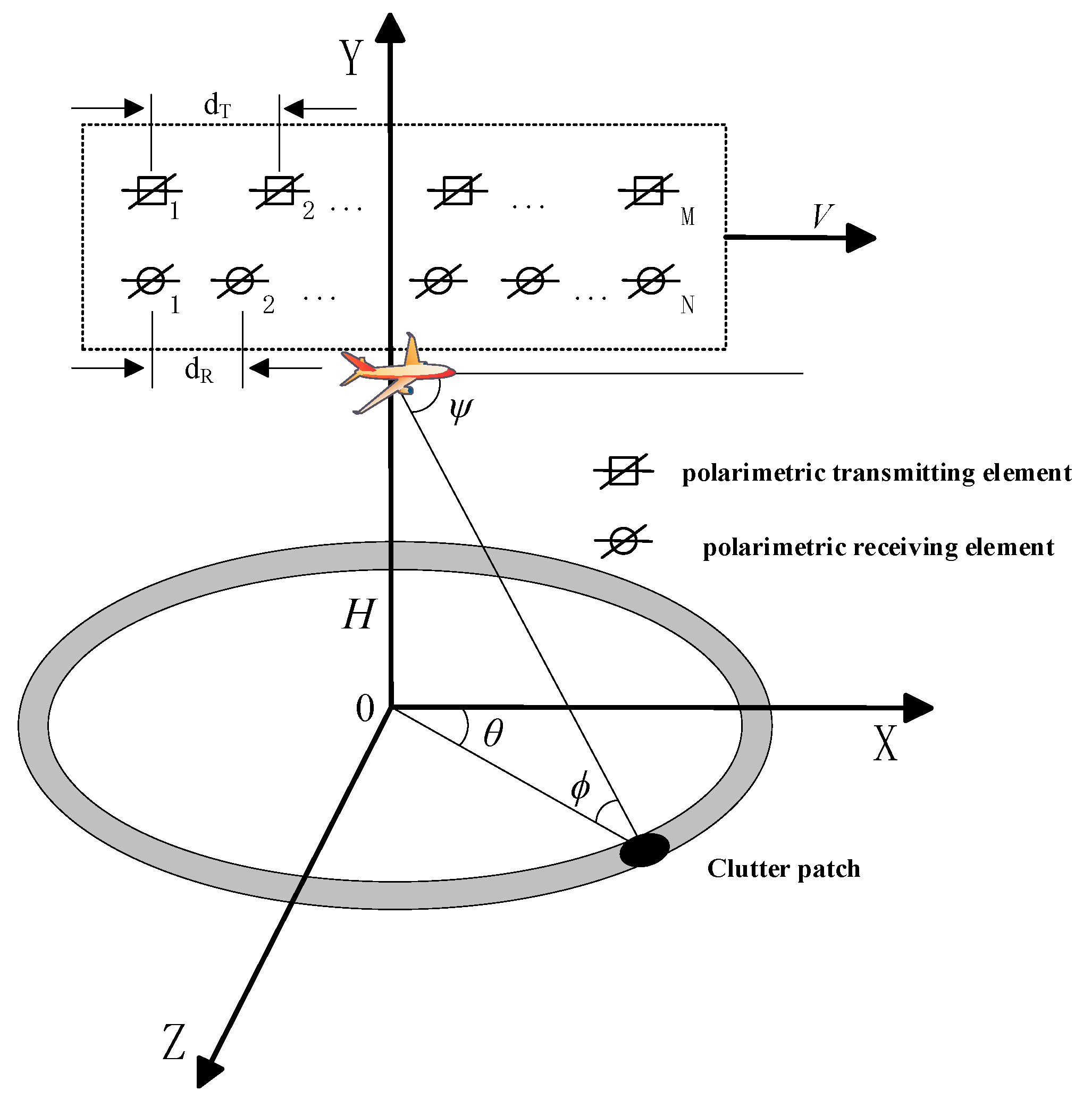
The signal model studied in this paper is based on an airborne FDA-P radar system with a co-located multiple-input multiple-output (MIMO) structure, as illustrated in Figure 1. It is assumed that the radar platform flies in a side-looking direction at an altitude $H$ and velocity $v$. During one coherent processing interval (CPI), there are $K$ coherent pulses. Along the flight direction, $M$ transmitting elements and $N$ receiving elements are arranged with spacings $d_T$ and $d_R$, respectively. Only horizontally polarized waveforms are radiated by the transmitting array elements; orthogonal dipole pairs are arranged at receiving elements to support horizontal-vertical dual-polarized reception and achieve polarization diversity. A fixed frequency increment $\Delta f$ is imposed between adjacent transmitting elements, with its value being small relative to the carrier frequency $f_0$ and to the transmitted waveform bandwidth. For the purpose of implementing transmit-array frequency diversity, each radiating element is configured with an individual carrier frequency $f_m=f_0+\left(m-1\right)\Delta f,m=1,2,\dots ,M$.

Define the transmitted normalized energy waveform of the $m$-th transmitting element as $z_m\left(t\right),0\le t\le T_p$. This waveform satisfies the unit energy constraint over the entire pulse duration: the total energy contained within one pulse width $T_p$ is equal to 1. To enable separation at the receiving end, these $M$ waveforms must be mutually orthogonal, i.e., for any $u,o\in \left[1,M\right]$:

$${\displaystyle {\int }_{T_p}{z}_u\left(t\right)}{z}_o^{\ast }\left(t\right)dt=\left\{\begin{array}{cc}1,\hfill & u=o\\ 0,\hfill & \mathrm{otherwise}\end{array}\right..$$

(1)

The actual complete signal $x_m\left(t\right)$ transmitted by the $m$-th element is given as:

$$x_m\left(t\right)=\sqrt{{\displaystyle \frac{E_t}{M}}}{z}_m\left(t\right)e^{j2\pi f_{m}t},$$

(2)

where $E_t$ denotes the total transmit energy.

For a far-field point scatterer, echo propagation delay arises jointly from the array spatial aperture, pulse transmission timing, and target radial motion. We analyze the two-way round-trip propagation delay of echo signals herein: signals are radiated from the $m$-th transmit array element, scattered by the target, and collected via the $n$-th receive array element at the time of the $k$-th transmitted pulse. Assuming the target is situated at equivalent slant range $r_{j,q}$ with spatial cone angle ${\psi }_{j,q,i}$, the overall two-way time delay is formulated as:

$${\tau }_{m,n,k}\left(r_{j,q},{\psi }_{j,q,i}\right)={\displaystyle \frac{1}{c}}\left[2r_{j,q}-d_T\left(m-1\right)\cos {\psi }_{j,q,i}\right.\left.-d_R\left(n-1\right)\cos {\psi }_{j,q,i}-2vT\left(k-1\right)\cos {\psi }_{j,q,i}\right].$$

(3)

In (3), $T$ denotes the pulse repetition interval, and $c$ represents the speed of light. The spatial cone angle ${\psi }_{j,q,i}$ is geometrically determined by the target’s azimuth angle ${\theta }_i$ and elevation angle ${\varphi }_{j,q}$, complying with the relation $\cos \left({\psi }_{j,q,i}\right)=\cos \left({\theta }_i\right)\cos \left({\varphi }_{j,q}\right)$. The equivalent slant distance for the $j$-th range gate under the $q$-th range ambiguity condition is expressed as $r_{j,q}=r_j+\left(q-1\right)r_u$. The maximum unambiguous detection range $r_u$ is constrained by the radar pulse repetition frequency $f_r$, calculated via the formula $r_u=c/\left(2f_r\right)$. Here, integer $q$ denotes the range ambiguity order, taking values from $1$ to $N_q$, and the parameter $N_q$ quantifies the overall quantity of ambiguous range zones within the detection scope.

The transmitted signal $x_m\left(t\right)$ propagates from the $m$-th transmitting element to the target, where it is modulated by the polarization scattering matrix $s={\left[s_{hh},s_{hv}\right]}^T$, and then propagates to the $n$-th receiving element, where $s_{hh}$ denotes $HH$ polarization (horizontal transmit, horizontal receive), and $s_{hv}$ denotes $HV$ polarization (horizontal transmit, vertical receive). The complex reflection coefficient corresponding to the $i$-th azimuth clutter patch within the $q$-th range ambiguity ring of the $j$-th range bin is denoted by ${\alpha }_{j,q,i}$, while $s_{hh}^{j,q,i}$ and $s_{hv}^{j,q,i}$ are defined as the polarimetric scattering coefficients. Then the total signal received at the port of the $n$-th receiving element is:

$$y_n\left(t\right)={\displaystyle \sum _{m=1}^M\left\{\sqrt{\frac{E_t}{M}}{\alpha }_{j,q,i}\left[\begin{array}{c}{s}_{hh}^{j,q,i}\\ s_{hv}^{j,q,i}\end{array}\right]z_m\left(t-{\tau }_{m,n,k}\right)e^{j2\pi f_m\left(t-{\tau }_{m,n,k}\right)}\right\}}.$$

(4)

3. Radar Data Pre-Processing

The received signal is multiplied by the receiver’s local oscillator signal $e^{-j2\pi f_{0}t}$, and then passes through a low-pass filter to remove high-frequency components:

$$y_n^{BB}\left(t\right)=y_n\left(t\right)e^{-j2\pi f_{0}t}.$$

(5)

By substituting the expression of $y_n\left(t\right)$ for the signal transmitted by the $m$-th element, the carrier term becomes:

$$e^{j2\pi f_m\left(t-{\tau }_{m,n,k}\right)}{e}^{-j2\pi f_{0}t}=e^{j2\pi \left(m-1\right)\Delta ft}{e}^{-j2\pi f_m{\tau }_{m,n,k}}.$$

(6)

Therefore, after down-conversion, the baseband form of the signal received at the $n$-th receiving element is:

$$y_n^{BB}\left(t\right)={\displaystyle \sum _{m=1}^M\left\{\sqrt{\frac{E_t}{M}}{\alpha }_{j,q,i}\left[\begin{array}{c}{s}_{hh}^{j,q,i}\\ s_{hv}^{j,q,i}\end{array}\right]z_m\left(t-{\tau }_{m,n,k}\right)e^{j2\pi \left(m-1\right)\Delta ft}{e}^{-j2\pi f_m{\tau }_{m,n,k}}\right\}}.$$

(7)

At the $H$ port and $V$ port of the $n$-th receiving element, a set of $M$ matched filters is connected, corresponding to the horizontally polarized transmitted waveforms. After matched filtering, two polarimetric output channels are obtained, namely the co-polarization channel $HH$ and the cross-polarization channel $HV$. The impulse response of the matched filter is the complex conjugate of the equivalent baseband signal of the transmitted waveform. Each filter corresponds to a specific transmitting element $m\in \left[1,M\right]$, with impulse response:

$$h_m\left(t\right)=z_m^{\ast }\left(-t\right)e^{-j2\pi \left(m-1\right)\Delta ft}.$$

(8)

For the $H$ port of the $n$-th receiving element, after the received signal passes through the matched filter for the $m$-th transmitting element, the output data after matched filtering are:

$$\begin{array}{ll}{y}_{n,H}^{(m)}\hfill & ={\displaystyle {\int }_{-\infty }^{\infty }{y}_{n,H}^{BB}}\left(t\right)h_m\left(t\right)dt\\ & ={\displaystyle {\int }_{-\infty }^{\infty }{\displaystyle \sum _{m^{\prime }=1}^M\left\{\sqrt{\frac{E_t}{M}}{\alpha }_{j,q,i}{s}_{hh}^{j,q,i}{z}_{m^{\prime }}\left(t-{\tau }_{m^{\prime },n,k}\right)e^{j2\pi \left(m^{\prime }-1\right)\Delta ft}{e}^{-j2\pi f_{m^{\prime }}{\tau }_{m^{\prime },n,k}}\right\}}}{z}_m^{\ast }\left(-t\right)e^{-j2\pi \left(m-1\right)\Delta ft}dt\hfill \end{array}.$$

(9)

According to the orthogonality condition of the transmitted waveforms, (9) can be rewritten as:

$$y_{n,H}^{\left(m\right)}=\sqrt{{\displaystyle \frac{E_t}{M}}}{\alpha }_{j,q,i}{s}_{hh}^{j,q,i}{e}^{-j2\pi f_m{\tau }_{m,n,k}}.$$

(10)

Similarly, for the $V$ port, applying the same matched filter $h_m(t)$ to the baseband signal $y_{n,V}^{BB}(t)$ yields the following:

$$y_{n,V}^{\left(m\right)}=\sqrt{{\displaystyle \frac{E_t}{M}}}{\alpha }_{j,q,i}{s}_{hv}^{j,q,i}{e}^{-j2\pi f_m{\tau }_{m,n,k}}.$$

(11)

Accordingly, after matched filtering of echoes from the $m$-th transmit element, $n$-th receive element, and $k$-th pulse, the resultant outputs are arranged into a $2\times 1$ column vector:

$$y_{m,n,k}=\sqrt{{\displaystyle \frac{E_t}{M}}}{\alpha }_{j,q,i}\left[\begin{array}{c}{s}_{hh}^{j,q,i}\\ s_{hv}^{j,q,i}\end{array}\right]e^{-j2\pi f_m{\tau }_{m,n,k}}.$$

(12)

Based on the above properties, the polarization scattering characteristic vector is obtained and used as the single-element polarization steering vector of the received signal:

$$a_p^{j,q,i}={\left[\begin{array}{cc}{s}_{hh}^{j,q,i}& s_{hv}^{j,q,i}\end{array}\right]}^T.$$

(13)

Thus, (12) can be expressed as:

$$y_{m,n,k}=\sqrt{{\displaystyle \frac{E_t}{M}}}{\alpha }_{j,q,i}{a}_p^{j,q,i}{e}^{-j2\pi f_m{\tau }_{m,n,k}}.$$

(14)

Substituting the expression for ${\tau }_{m,n,k}\left(r_{j,q},{\psi }_{j,q,i}\right)$, we expand the phase term:

$$e^{-j2\pi f_m{\tau }_{m,n,k}}=e^{-j{\displaystyle \frac{4\pi f_m{r}_{j,q}}{c}}}\cdot e^{j{\displaystyle \frac{2\pi f_m\left(m-1\right)d_T\cos {\psi }_{j,q,i}}{c}}}\cdot e^{j{\displaystyle \frac{2\pi f_m\left(n-1\right)d_R\cos {\psi }_{j,q,i}}{c}}}\cdot e^{j{\displaystyle \frac{4\pi f_m\left(k-1\right)vT\cos {\psi }_{j,q,i}}{c}}}.$$

(15)

Based on $f_m=f_0+\left(m-1\right)\Delta f$:

$$\begin{array}{ll}{e}^{-j2\pi f_m{\tau }_{m,n,k}}& =\left[e^{-j{\displaystyle \frac{4\pi f_0{r}_{j,q}}{c}}}{e}^{-j{\displaystyle \frac{4\pi \left(m-1\right)\Delta f{r}_{j,q}}{c}}}\right]\left[e^{j{\displaystyle \frac{2\pi f_0\left(m-1\right)d_T\cos {\psi }_{j,q,i}}{c}}}{e}^{j{\displaystyle \frac{2\pi \left(m-1\right)\Delta f\left(m-1\right)d_T\cos {\psi }_{j,q,i}}{c}}}\right]\hfill \\ & \times \left[e^{j{\displaystyle \frac{2\pi f_0\left(n-1\right)d_R\cos {\psi }_{j,q,i}}{c}}}{e}^{j{\displaystyle \frac{2\pi \left(m-1\right)\Delta f\left(n-1\right)d_R\cos {\psi }_{j,q,i}}{c}}}\right]\hfill \\ & \times \left[e^{j{\displaystyle \frac{4\pi f_0\left(k-1\right)vT\cos {\psi }_{j,q,i}}{c}}}{e}^{j{\displaystyle \frac{4\pi \left(m-1\right)\Delta f\left(k-1\right)vT\cos {\psi }_{j,q,i}}{c}}}\right]\hfill \end{array}.$$

(16)

Since $\left(M-1\right)\Delta f/f_0\ll 1$, the terms $e^{j2\pi \left(m-1\right)\Delta f\left(m-1\right)d_T\cos {\psi }_{j,q,i}/c}$, $e^{j2\pi \left(m-1\right)\Delta f\left(n-1\right)d_R\cos {\psi }_{j,q,i}/c}$, and $e^{j4\pi \left(m-1\right)\Delta f\left(k-1\right)vT\cos {\psi }_{j,q,i}/c}$ may be safely neglected in the phase expansion process.

Remark 1.

In a typical FDA radar, the frequency increment $\Delta f$ must satisfy $\Delta f\ll f_0/\left(M-1\right)$ to maintain the spatial coherence of the transmit array, under which the ratio $\left(M-1\right)\Delta f/f_0$ is typically on the order of ${10}^{-6}$ to ${10}^{-5}$. To quantify the approximation error, we examine the maximum residual phase error introduced by neglecting the term $e^{j2\pi \left(m-1\right)\Delta f\left(m-1\right)d_T\cos {\psi }_{j,q,i}/c}$, which is bounded by ${\left|{\varphi }_{err}\right|}_{\max }=2\pi {\left(M-1\right)}^2\Delta f{d}_T/c$. Substituting typical parameters ($M=4$, $\Delta f=250\mathrm{Hz}$, $d_T=0.15\mathrm{m}$, $c=3\times {10}^8\mathrm{m}/\mathrm{s}$) yields ${\left|{\varphi }_{err}\right|}_{\max }\approx 7.07\times {10}^{-6}\mathrm{rad}$, which is on the order of ${10}^{-6}$ radians. This is far below the typical phase resolution of airborne radar systems, which is generally on the order of ${10}^{-2}$ to ${10}^{-3}$ radians for practical systems, and thus has no appreciable impact on the steering vector accuracy or the final SINR loss performance. The same bound applies to the receive and Doppler domain terms, as they share the same mathematical structure. Therefore, neglecting these terms is well justified and does not compromise the fidelity of the derived signal model.

Furthermore, the global common phase factor $e^{-j4\pi f_0{r}_{j,q}/c}$ can be merged into the amplitude coefficient $\alpha$. Based on the above approximations, three key frequency components are obtained as follows:

$$\begin{array}{l}{f}_T\left(r_{j,q},{\psi }_{j,q,i}\right)=-2\Delta f{r}_{j,q}/c+d_T\cos {\psi }_{j,q,i}/{\lambda }_0\\ f_R\left({\psi }_{j,q,i}\right)=d_R\cos {\psi }_{j,q,i}/{\lambda }_0\\ f_D\left({\psi }_{j,q,i}\right)=2vT\cos {\psi }_{j,q,i}/{\lambda }_0\end{array},$$

(17)

where $f_T\left(r_{j,q},{\psi }_{j,q,i}\right)$, $f_R\left({\psi }_{j,q,i}\right)$, and $f_D\left({\psi }_{j,q,i}\right)$ denote the transmit spatial frequency, receive spatial frequency, and platform-induced Doppler frequency, respectively. Combining all phase terms, the output after matched filtering is:

$$y_{m,n,k}=\sqrt{{\displaystyle \frac{E_t}{M}}}{\alpha }_{j,q,i}{a}_p^{j,q,i}{e}^{j2\pi \left(m-1\right)f_T\left(r_{j,q},{\psi }_{j,q,i}\right)}{e}^{j2\pi \left(n-1\right)f_R\left({\psi }_{j,q,i}\right)}{e}^{j2\pi \left(k-1\right)f_D\left({\psi }_{j,q,i}\right)}.$$

(18)

By summing all results obtained through matched filtering, echoes reflected from any clutter scatterer can be represented in a joint four-dimensional space comprising the transmit spatial, receive spatial, temporal, and polarization domains. Throughout this paper, the joint steering vectors and covariance matrices are arranged in the order of transmit, receive, Doppler, and polarization dimensions:

$$y=\sqrt{{\displaystyle \frac{E_t}{M}}}{\alpha }_{j,q,i}{a}_T\left(f_T\left(r_{j,q},{\psi }_{j,q,i}\right)\right)\otimes a_R\left(f_R\left({\psi }_{j,q,i}\right)\right)\otimes a_D\left(f_D\left({\psi }_{j,q,i}\right)\right)\otimes a_p^{j,q,i},$$

(19)

where $a_T\left(f_T\left(r_{j,q},{\psi }_{j,q,i}\right)\right)\in {ℂ}^{M\times 1}$ is the transmit steering vector, $a_R\left(f_R\left({\psi }_{j,q,i}\right)\right)\in {ℂ}^{N\times 1}$ is the receive steering vector, and $a_D\left(f_D\left({\psi }_{j,q,i}\right)\right)\in {ℂ}^{K\times 1}$ is the Doppler steering vector, respectively expressed as:

$$\begin{array}{l}{a}_T\left(f_T\left(r_{j,q},{\psi }_{j,q,i}\right)\right)={\left[1,e^{j2\pi f_T\left(r_{j,q},{\psi }_{j,q,i}\right)},\dots ,e^{j2\pi f_T\left(r_{j,q},{\psi }_{j,q,i}\right)\left(M-1\right)}\right]}^T\\ a_R\left(f_R\left({\psi }_{j,q,i}\right)\right)={\left[1,e^{j2\pi f_R\left({\psi }_{j,q,i}\right)},\dots ,e^{j2\pi f_R\left({\psi }_{j,q,i}\right)\left(N-1\right)}\right]}^T\\ a_D\left(f_D\left({\psi }_{j,q,i}\right)\right)={\left[1,e^{j2\pi f_D\left({\psi }_{j,q,i}\right)},\dots ,e^{j2\pi f_D\left({\psi }_{j,q,i}\right)\left(K-1\right)}\right]}^T\end{array}.$$

(20)

The polarimetric space–time clutter snapshot for the $j$-th range bin is obtained by arranging the matched-filtered outputs $y_{m,n,k}$ sequentially along the transmit, receive, and pulse dimensions. The returns from all clutter patches within the same range cell are then accumulated, yielding the following expression:

$$x_c={\displaystyle \sum _{q=1}^{N_q}{\displaystyle \sum _{i=1}^{N_c}\left\{\sqrt{\frac{E_t}{M}}{\alpha }_{j,q,i}{a}_T\left(f_T\left(r_{j,q},{\psi }_{j,q,i}\right)\right)\otimes a_R\left(f_R\left({\psi }_{j,q,i}\right)\right)\otimes a_D\left(f_D\left({\psi }_{j,q,i}\right)\right)\otimes a_p^{j,q,i}\right\}}},$$

(21)

where $N_c$ denotes the number of discrete clutter patches uniformly sampled in azimuth within each range ring.

Scattered echoes from point targets are fully polarized waves. We define the intrinsic polarization steering vector of the target echoes as:

$$a_p^0\left({\gamma }_0,{\eta }_0\right)={\left[\cos {\gamma }_0,\sin {\gamma }_0{e}^{j{\eta }_0}\right]}^T,$$

(22)

where two variables ${\gamma }_0$ and ${\eta }_0$ jointly characterize the polarization state of target backscattering signals within range-ambiguous zones. Concretely, ${\gamma }_0$ denotes the amplitude ratio between horizontal and vertical polarization receiving channels, while ${\eta }_0$ is the phase difference across these two orthogonal $H/V$ channels. For any moving target located inside a range-ambiguous region, we denote its echo complex amplitude as ${\alpha }_0$, slant range as $r_0$, radial line-of-sight velocity as $v_0$, and spatial cone angle as ${\psi }_0$. Under these preset parameters, the complete polarimetric space–time joint steering vector corresponding to this moving target is given by the following formula:

$$a_0=a_T\left(f_T^0\left(r_0,{\psi }_0\right)\right)\otimes a_R\left(f_R^0\left({\psi }_0\right)\right)\otimes a_D\left(f_D^0\left({\psi }_0,v_0\right)\right)\otimes a_p^0\left({\gamma }_0,{\eta }_0\right),$$

(23)

where $f_D^0\left({\psi }_0,v_0\right)=2vT\cos {\psi }_0/{\lambda }_0+2v_{0}T/{\lambda }_0$ is the normalized Doppler frequency of the target, accounting for both the platform motion and the target’s radial velocity. The corresponding target echo signal snapshot $x_0$ can be written as:

$$x_0={\alpha }_0{a}_T\left(f_T^0\left(r_0,{\psi }_0\right)\right)\otimes a_R\left(f_R^0\left({\psi }_0\right)\right)\otimes a_D\left(f_D^0\left({\psi }_0,v_0\right)\right)\otimes a_p^0\left({\gamma }_0,{\eta }_0\right).$$

(24)

Therefore, the received data of the $j$-th range cell, containing the moving target, clutter, and white noise, can be expressed as:

$$x_j=x_c+x_0+n,$$

(25)

where $n$ is the noise component, which is assumed to be zero-mean Gaussian white noise, independent across both spatial and temporal dimensions.

From (17), the original transmit spatial frequency of the $m$-th transmitting element is linearly related to the target’s reference slant range $r_j$ and can be specifically expressed as:

$$\begin{array}{cc}{f}_T\left(r_{j,q},{\psi }_{j,q,i}\right)& ={\displaystyle \frac{-2\Delta f{r}_{j,q}}{c}}+{\displaystyle \frac{d_T\cos {\psi }_{j,q,i}}{{\lambda }_0}}\hfill \\ & =-{\displaystyle \frac{2\Delta f{r}_j}{c}}-{\displaystyle \frac{2\Delta f{r}_u}{c}}\left(q-1\right)+{\displaystyle \frac{d_T\cos {\psi }_{j,q,i}}{{\lambda }_0}}\hfill \end{array}.$$

(26)

The space–time spectrum of clutter shifts across range gates, a phenomenon known as the range-dependence effect. To address this issue, Ref. [33] proposed the secondary range-dependent compensation method. Its essential idea is to establish a transmit-domain compensation vector that cancels the range-coupled component in the clutter’s transmit spatial frequency. This vector can be expressed by:

$$u_T\left(r_j\right)={\left[1,e^{-j{\displaystyle \frac{4\pi \Delta f}{c}}{r}_j},\dots ,e^{-j{\displaystyle \frac{4\pi \Delta f}{c}}{r}_j\left(M-1\right)}\right]}^T.$$

(27)

The above compensation is restricted to correcting the range dependence in the transmit spatial frequency, while remaining independent of the receive spatial, Doppler, and polarization domains. Extending this vector to the complete transmit, receive, pulse, and polarization space yields the full-data compensation matrix, given by:

$$U\left(r_j\right)=\mathrm{diag}\left\{u_T\left(r_j\right)\otimes 1_N\otimes 1_K\right\}\otimes I_P,$$

(28)

where the factor $p=2$ accounts for the two receive polarization channels. The compensated data snapshot is ${\widehat{x}}_j=U{\left(r_j\right)}^H{x}_j$. Following compensation, the transmit frequency is determined exclusively by the range ambiguity index $q$, and is unaffected by the reference slant range $r_j$ of the $j$-th range gate.

$${\widehat{f}}_T\left(q,{\psi }_{j,q,i}\right)=-{\displaystyle \frac{2\Delta f{r}_u}{c}}\left(q-1\right)+{\displaystyle \frac{d_T\cos {\psi }_{j,q,i}}{{\lambda }_0}}.$$

(29)

Consequently, the compensated clutter data for the $j$-th range cell can be expressed as:

$$\begin{array}{ll}{\widehat{x}}_c& =U{\left(r_j\right)}^H{x}_c\hfill \\ & ={\displaystyle \sum _{q=1}^{N_q}{\displaystyle \sum _{i=1}^{N_c}\left\{\sqrt{\frac{E_t}{M}}{\alpha }_{j,q,i}{a}_T\left({\widehat{f}}_T\left(q,{\psi }_{j,q,i}\right)\right)\otimes a_R\left(f_R\left({\psi }_{j,q,i}\right)\right)\otimes a_D\left(f_D\left({\psi }_{j,q,i}\right)\right)\right\}\otimes a_p^{j,q,i}}}\hfill \end{array}.$$

(30)

After compensation, the complete received radar data for the $j$-th range cell can be expressed uniformly as follows:

$${\widehat{x}}_j={\widehat{x}}_c+{\widehat{x}}_0+\widehat{n},$$

(31)

where ${\widehat{x}}_0=U{\left(r_j\right)}^H{x}_0$, $\widehat{\mathbf{n}}$ denotes white Gaussian noise with power ${\sigma }_n^2$. It is worth noting that the received data for the $j$-th range cell contain contributions from multiple range-ambiguity regions due to the high-PRF operation. The exact ambiguity index of any potential target is unknown a priori and must be jointly estimated along with the angle and Doppler parameters of the target.

4. FDA-PSTAP Algorithm

4.1. The Conventional Full-Dimension FDA-PSTAP

Assume that the target, clutter, and noise are statistically independent of each other. The polarimetric space–time clutter covariance matrix for the airborne FDA-P radar is obtained as:

$$\begin{array}{ll}{\widehat{R}}_{P-S-T}& =E\left[{\widehat{x}}_c{\widehat{x}}_c^H\right]\hfill \\ & ={\displaystyle \sum _{q=1}^{N_q}{\displaystyle \sum _{i=1}^{N_c}\frac{E_t}{M}}}E\left[{\left|{\alpha }_{j,q,i}\right|}^2\right]\hfill \\ & \times \left[a_T\left({\widehat{f}}_T\left(q,{\psi }_{j,q,i}\right)\right)a_T^H\left({\widehat{f}}_T\left(q,{\psi }_{j,q,i}\right)\right)\otimes a_R\left(f_R\left({\psi }_{j,q,i}\right)\right)a_R^H\left(f_R\left({\psi }_{j,q,i}\right)\right),\right.\hfill \\ & \left.\otimes a_D\left(f_D\left({\psi }_{j,q,i}\right)\right)a_D^H\left(f_D\left({\psi }_{j,q,i}\right)\right)\right]\otimes \left[a_p^{j,q,i}{\left(a_p^{j,q,i}\right)}^H\right]\hfill \\ & ={\widehat{R}}_{S-T}\otimes R_P\hfill \end{array}$$

(32)

where ${\widehat{R}}_{S-T}$ is the space–time clutter covariance matrix and $R_p$ is the polarization clutter covariance matrix.

Remark 2.

The derivation of the above formula is as follows. The clutter snapshot is first expanded as a sum of contributions from individual clutter patches. After expanding the outer product and applying the Kronecker product property, the space–time part and the polarization part are separated. Under the standard assumption that echoes from different clutter patches are uncorrelated, all cross-terms vanish, leaving only the auto-terms. Then, by invoking the statistical independence between the clutter amplitudes and the steering vectors, the expectation is distributed over each factor. Since the polarization covariance matrix is independent of the patch indices, it is extracted from the summation over clutter patches. Finally, the remaining space–time summation is defined as the space–time covariance matrix ${\widehat{R}}_{S-T}$, and the polarization covariance matrix is denoted as $R_p$, yielding the Kronecker product factorization.

The factorization in (32) relies on the standard separability assumption widely adopted in the polarimetric STAP literature [7,34,35], i.e., the polarization scattering characteristics of clutter are statistically independent of its space–time response. This assumption is generally valid in homogeneous clutter environments with properly calibrated polarization channels. Specifically, this can be expressed as:

$$R_p=E\left[a_p^{j,q,i}{\left(a_p^{j,q,i}\right)}^H\right]=\left[\begin{array}{cc}E\left({\left|s_{hh}^{j,q,i}\right|}^2\right)& E\left(s_{hh}^{j,q,i}{\left(s_{hv}^{j,q,i}\right)}^{\ast }\right)\\ E\left(s_{hv}^{j,q,i}{\left(s_{hh}^{j,q,i}\right)}^{\ast }\right)& E\left({\left|s_{hv}^{j,q,i}\right|}^2\right)\end{array}\right].$$

(33)

Let $\xi =E\left(|s_{hv}^{j,q,i}{|}^2\right)/E\left(|s_{hh}^{j,q,i}{|}^2\right)$ stand for the average power ratio between the $V$ and the $H$ receiving channel; $E\left(s_{hh}^{j,q,i}{\left(s_{hv}^{j,q,i}\right)}^{\ast }\right)=\varpi \sqrt{E\left(|s_{hh}^{j,q,i}{|}^2\right)E\left(|s_{hv}^{j,q,i}{|}^2\right)}{e}^{-j\rho }$, where $\rho$ refers to the average phase deviation between the two channels; $\varpi$ is defined as the correlation coefficient between the two channels; and the designations $\varpi =0$, $0<\varpi <1$, and $\varpi =1$ correspond to unpolarized, partially polarized, and fully polarized clutter, respectively. Therefore, $R_p$ can be written in a normalized form:

$$R_p={\displaystyle \frac{1}{1+\xi }}\left[\begin{array}{cc}1& \sqrt{\xi }\varpi e^{-j\rho }\\ \sqrt{\xi }\varpi e^{j\rho }& \xi \end{array}\right].$$

(34)

The complete polarimetric space–time CNCM then takes the following form:

$$R_{cn}={\widehat{R}}_{S-T}\otimes R_P+{\sigma }_n^2{I}_{2MNK}={\widehat{R}}_{P-S-T}+{\sigma }_n^2{I}_{2MNK},$$

(35)

The factor $2$ accounts for the two received polarization channels. With the compensated transmit spatial frequency from Equation (29) taken into account, the target steering vector is modified as follows:

$${\widehat{a}}_0=a_T\left({\widehat{f}}_T^0\left(q_0,{\psi }_0\right)\right)\otimes a_R\left(f_R^0\left({\psi }_0\right)\right)\otimes a_D\left(f_D^0\left({\psi }_0,v_0\right)\right)\otimes a_p^0\left({\gamma }_0,{\eta }_0\right).$$

(36)

For airborne radar, with $R_{cn}$ as the polarimetric space-time clutter-plus-noise covariance matrix and ${\widehat{a}}_0$ as the target polarimetric space-time steering vector, the optimal weight vector is given by:

$$w={\displaystyle \frac{R_{cn}^{-1}{\widehat{a}}_0}{{\widehat{a}}_0^H{R}_{cn}^{-1}{\widehat{a}}_0}}.$$

(37)

In practice, the ideal CNCM $R_{cn}$ in (37) is not known a priori. It is therefore necessary to estimate it from a finite number of training samples, which must be independent and identically distributed. Thus, the samples ${\left\{{\widehat{x}}_j\right\}}_{j=1}^J$ can be used to build the sample covariance matrix (SCM):

$${\widehat{R}}_f={\displaystyle \sum _{j=1}^J{\widehat{x}}_j{\widehat{x}}_j^{\mathrm{H}}},$$

(38)

where $J$ denotes the number of training samples. We substitute the ideal $R_{cn}$ in Equation (37) with ${\widehat{R}}_f$ from Equation (38), and incorporate the compensated target steering vector ${\widehat{a}}_0$; then the full-dimensional (FD) FDA-PSTAP weight vector based on the SCM is given by:

$$\widehat{w}={\displaystyle \frac{{\widehat{R}}_f^{-1}{\widehat{a}}_0}{{\widehat{a}}_0^H{\widehat{R}}_f^{-1}{\widehat{a}}_0}}.$$

(39)

Therefore, the output power following adaptive processing is given by:

$$P\left(\widehat{w}\right)={\displaystyle \frac{{\widehat{a}}_0^H{\widehat{R}}_f^{-1}{\widehat{\mathit{R}}}_f{\widehat{R}}_f^{-1}{\widehat{a}}_0}{{\left[{\widehat{a}}_0^H{\widehat{R}}_f^{-1}{\widehat{a}}_0\right]}^2}}.$$

(40)

Equation (40) reveals that the FDA-PSTAP processor performs well, provided that the estimated inverse covariance matrix ${\widehat{R}}_f^{-1}$ is close to the true $R_{cn}^{-1}$. Unfortunately, the training sample size available in real applications is usually too small to satisfy the RMB criterion [36]. In this situation, the mismatch between ${\widehat{R}}_f^{-1}$ and $R_{cn}^{-1}$ grows markedly, which causes a severe increase in output power $P\left(\widehat{w}\right)$ and thereby impairs the clutter rejection performance.

4.2. Reduced-Dimensional FDA-PSTAP

As demonstrated in the previous subsection, the FD-FDA-PSTAP suffers from severe performance degradation in practical environments with limited training samples. Therefore, this paper proposes an effective FDA-PSTAP to overcome the issue of limited training samples. In the FDA-PSTAP setting where range-ambiguous clutter prevails, the clutter returns from different ambiguous range intervals are almost uncorrelated with one another, as reported in [33]. This characteristic naturally allows each ambiguous region to be handled separately, incurring virtually no performance degradation. Therefore, secondary training samples acquired from range cells outside the current interval carry little useful information for the estimation task. Consequently, we develop a reduced-dimensional (RD) FDA-PSTAP for clutter suppression under limited training samples.

Unlike classical two-dimensional localization approaches, the proposed scheme offers two prominent advantages. First, it fully leverages the inherent range-sensing capability of the FDA transmit dimension by treating range as an independent localization dimension. Second, all degrees of freedom in the polarimetric dimension are intentionally preserved in the dimensionality reduction process, ensuring that the system fully preserves the target’s polarimetric scattering characteristics.

Assume the target is located in the $q_0$-th range ambiguity region, with a spatial cone angle of ${\psi }_0$, a radial velocity of $v_0$, and a normalized Doppler frequency of $f_D^0\left({\psi }_0,v_0\right)$. For clarity of presentation, the following derivation is carried out for a single hypothesized ambiguity region indexed by $q_0$. In actual processing, this procedure is repeated for each possible $q$ (e.g., $q=1,2,\dots ,N_q$) to form a bank of reduced-dimension transformation matrices. The processor then evaluates the output power for each hypothesized $q$, and a peak across the resulting range-ambiguity-angle-Doppler space indicates the presence and location of the target. This hypothesis-testing framework ensures that no prior knowledge of the true ambiguity region is required. In this paper, in the transmit, receive, and Doppler domains, respectively, we take $J_1,J_2,J_3$ adjacent beams centered at the target parameters to construct reduced-dimensional basis matrices. According to the RMB criterion, the reduced-dimensional parameters $J_1,J_2,J_3$ must satisfy $D\ge 2\times \left(J_1{J}_2{J}_{3}P\right)$ to ensure reliable covariance matrix estimation, where $D$ is the number of available training samples.

Transmit-domain local basis matrix:

$$L_T=\left[a_T\left({\widehat{f}}_T^0\left(q_0,{\psi }_0\right)\right),a_T{\widehat{f}}_T^0\left(q_0,{\psi }_1\right),\dots ,a_T\left({\widehat{f}}_T^0\left(q_0,{\psi }_{J_1-1}\right)\right)\right]\in {ℂ}^{M\times J_1}.$$

(41)

Receive-domain local basis matrix:

$$L_R=\left[a_R\left(f_R^0\left({\psi }_0\right)\right),a_R^0\left(f_R\left({\psi }_1\right)\right),\dots ,a_R\left(f_R^0\left({\psi }_{J_2-1}\right)\right)\right]\in {ℂ}^{N\times J_2}.$$

(42)

Doppler-domain local basis matrix:

$$L_D=\left[a_D\left(f_D^0\left({\psi }_0,v_0\right)\right),a_D\left(f_D^0\left({\psi }_0,v_1\right)\right),\dots ,a_D\left(f_D^0\left({\psi }_0,v_{J_3-1}\right)\right)\right]\in {ℂ}^{K\times J_3}.$$

(43)

In order to preserve the complete polarization information contained in both the $HH$ and $HV$ receiving channels, the reduced-dimensional matrices in the range, angle, and Doppler domains are Kronecker product with the polarization identity matrix, resulting in the polarization-preserving total dimensionality-reduction transform matrix:

$$T=\left(L_T\otimes L_R\otimes L_D\right)\otimes I_P.$$

(44)

For the purpose of alleviating both the covariance-matrix estimation error caused by limited training samples and the computational cost, a linear dimensionality reduction transformation can be performed on the full-dimensional data. We then denote the reduced-dimensional samples, steering vector, and covariance matrix as:

$$x_{RD}=T^H{\widehat{x}}_l,a_{RD}=T^H{\widehat{a}}_0,R_{RD}=T^H{\widehat{R}}_{f}T.$$

(45)

According to the minimum variance distortionless response (MVDR) criterion:

$$\begin{array}{l}\underset{w_{RD}}{\min }{w}_{RD}^H{R}_{RD}{w}_{RD}\\ \mathrm{s}.\mathrm{t}.w_{RD}^H{a}_{RD}=1\end{array}.$$

(46)

Then, the optimal RD-FDA-PSTAP is given as:

$$w_{RD}={\displaystyle \frac{R_{RD}^{-1}{a}_{RD}}{a_{RD}^H{R}_{RD}^{-1}{a}_{RD}}}.$$

(47)

Under limited snapshots, the optimal FDA-PSTAP in (39) will be replaced by

$${\widehat{w}}_{RD}={\displaystyle \frac{{\widehat{R}}_{f,RD}^{-1}{a}_{RD}}{a_{RD}^H{\widehat{R}}_{f,RD}^{-1}{a}_{RD}}},$$

(48)

where ${\widehat{R}}_{f,RD}=T^H{\widehat{R}}_{f}T$.

In practical situations, the RD DOFs $J_1{J}_2{J}_{3}P$ are much smaller than $MNKP$. Since $D=MNKP$ satisfies the RMB requirement for the reduced-dimensional processor ($D\ge J_1{J}_2{J}_{3}P$), the reduced-dimensional covariance matrix can be well estimated, and the performance of RD-FDA-PSTAP can approach that of the optimal processor. Hence, RD-FDA-PSTAP achieves effective performance under limited training samples.

5. Numerical Experiments

This section presents a series of experiments to illustrate the efficacy of the RD-FDA-PSTAP method. The experimental settings are summarized in

Table 1. Parameter settings.

Parameter	Value	Unit
Height	6000	m
Wavelength	0.30	m
Transmitting element number	4	/
Receiving element number	4	/
Receiving element spacing	0.15	m
Transmitting element spacing	0.15	m
Pulse number	4	/
Frequency shifting	250	Hz
Pulse repetition frequency	2000	Hz
Polarization dimension	2	/
Polarization correlation coefficient	1	/
H/V clutter power ratio	1	/
Statistical phase difference	1.57	rad
Clutter patch number	360	/
Number of range ambiguity regions	2	/
CNR	30	dB

. In particular, we employ a polarization-preserving localized dimensionality reduction method with $J_1=J_2=J_3=3$, while normalizing the noise power to 0 dB and setting the number of range ambiguity regions to two. The noise power is normalized to 0 dB, which is a standard convention in FDA-MIMO and STAP literature [37]. This normalization does not affect the output SINR loss, as the loss is determined by the relative power ratios rather than the absolute noise level. To thoroughly verify the adaptability of the proposed algorithm under different clutter environments, platform velocities of $V=150\mathrm{m}/\mathrm{s}$ and $V=300\mathrm{m}/\mathrm{s}$ are considered. Meanwhile, to further validate the robustness of the proposed algorithm, different target polarization states $\left({\gamma }_0,{\eta }_0\right)$ and numbers of training samples ($D=MNKP$ and $D=2MNKP$) are also taken into account. It is further assumed that the clutter powers in the two receive polarization channels are equal, i.e., $\xi =1$, and the phase difference is $\rho =90°$.

It is also verified that, under the above parameters, the condition $\left(M-1\right)\Delta f/f_0\approx 7.5\times {10}^{-7}\ll 1$ is strictly satisfied, and the maximum phase error introduced by the approximation in Equations (16) and (17) is on the order of ${10}^{-6}$ radians, confirming the validity of the derived signal model.

We evaluate the performance of different FDA-PSTAP approaches based on the output SINR loss. For the optimal FDA-PSTAP, its SINR loss is defined as:

$${\mathrm{SIN}\mathrm{R}}_{\mathrm{Loss}}^{\mathrm{optimal}\mathrm{FDA}\mathrm{PSTAP}}={\displaystyle \frac{P_n}{MNKP}}{\displaystyle \frac{{\left|w_{opt}^H{a}_0\right|}^2}{w_{opt}^H{R}_{cn}{w}_{opt}}}.$$

(49)

The SINR losses for the FD-FDA-PSTAP and the RD-FDA-PSTAP are computed similarly, using their respective weight vectors, which are derived from the sample covariance matrix and the reduced-dimension transformation matrix. The final output SINR loss is computed by averaging the results over 100 independent Monte Carlo trials.

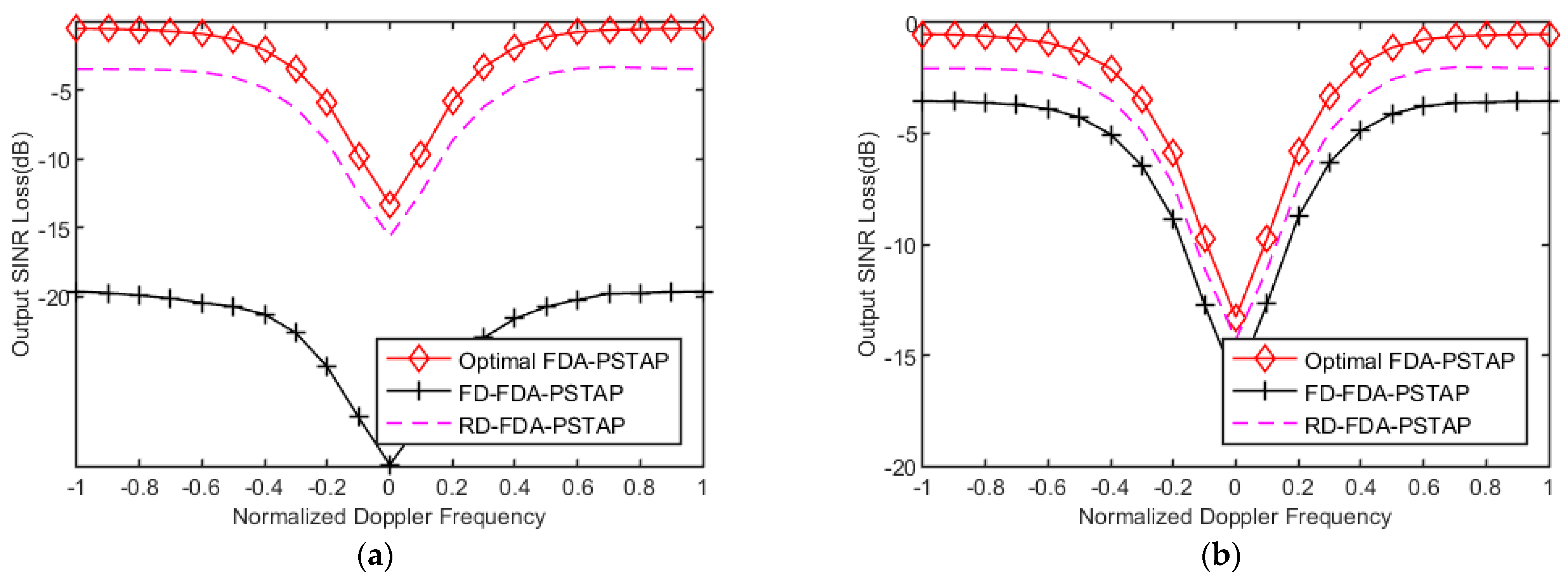
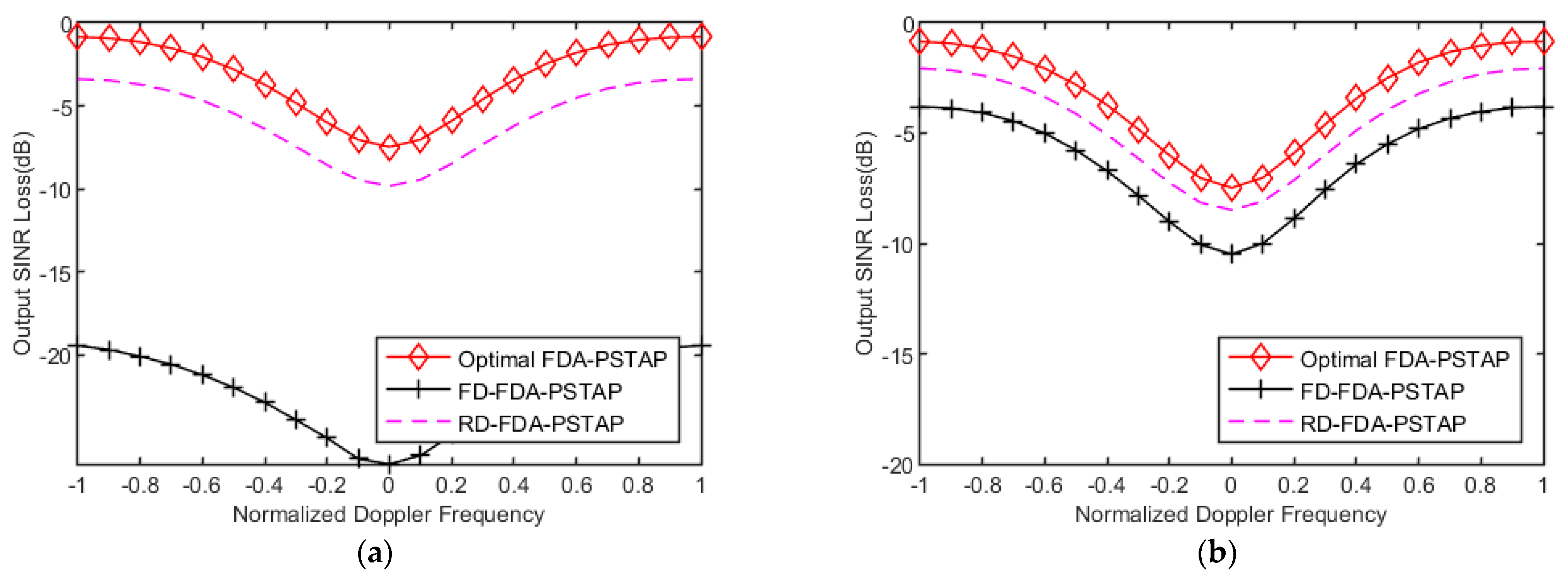
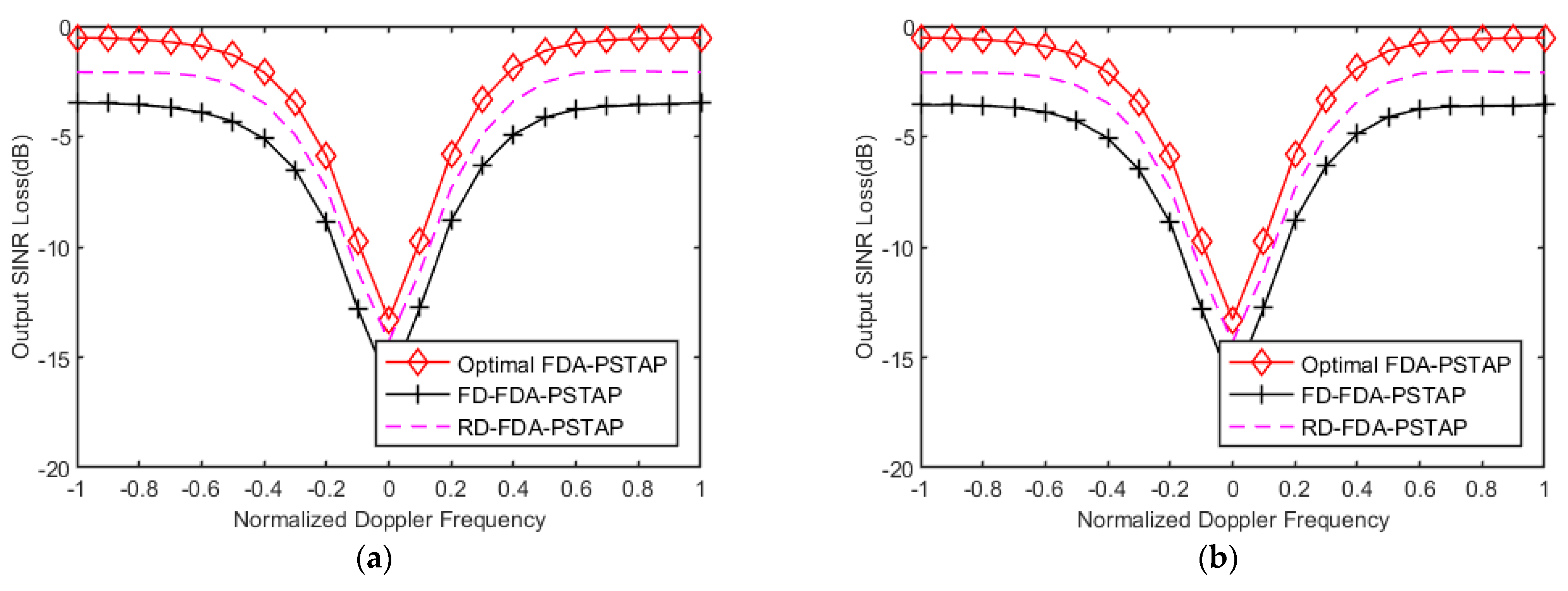
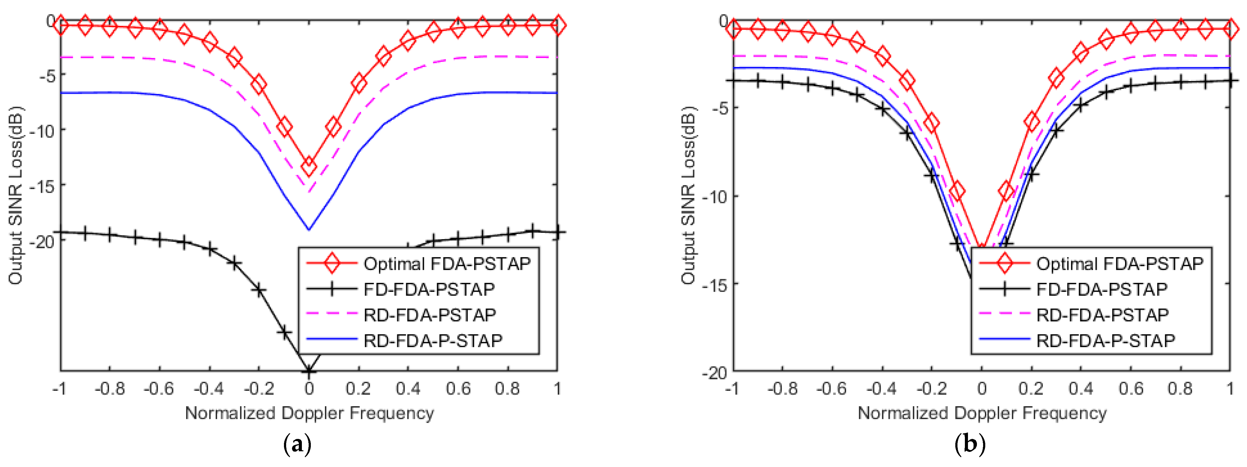
Figure 2 plots the output SINR loss versus normalized Doppler frequency under the conditions $V=150\mathrm{m}/\mathrm{s}$ and target polarization $\left({\gamma }_0,{\eta }_0\right)=\left(45°,65°\right)$. For the case with training sample number $D=MNKP$, the FD-FDA-PSTAP suffers severe performance degradation owing to inaccurate covariance matrix estimation caused by insufficient training samples. Its SINR loss exceeds 20 dB around the zero-Doppler clutter ridge where clutter power reaches the maximum. By contrast, the proposed RD-FDA-PSTAP maps full-dimensional data into a much lower-dimensional subspace, achieving substantial performance improvement. It reduces the required degrees of freedom from $MNKP$ to $J_1{J}_2{J}_{3}P$ and effectively alleviates sample starvation. Across most Doppler bins, its SINR loss is 15–17 dB lower than that of FD-FDA-PSTAP, with the most obvious gap appearing in the main clutter region. When the training samples are doubled to the case $D=2MNKP$, as illustrated in Figure 2b, both algorithms improve covariance estimation accuracy. The FD-FDA-PSTAP achieves considerable performance recovery, with its SINR loss reduced by approximately 16 dB compared with the $D=MNKP$ scenario. Meanwhile, RD-FDA-PSTAP further approaches the optimal performance, whose SINR loss is merely 1–2 dB away from the theoretical optimum over the entire Doppler spectrum. These results verify that RD-FDA-PSTAP exhibits robust performance with severely limited training samples and can maintain near-optimal clutter suppression with adequate samples. Benefiting from the polarization-preserving transformation, no polarimetric discrimination information is lost during dimensionality reduction.

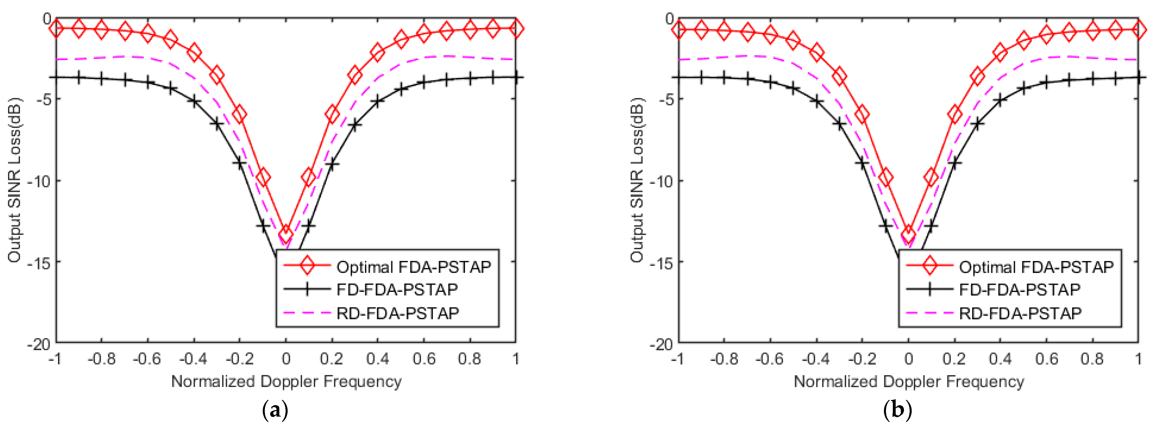
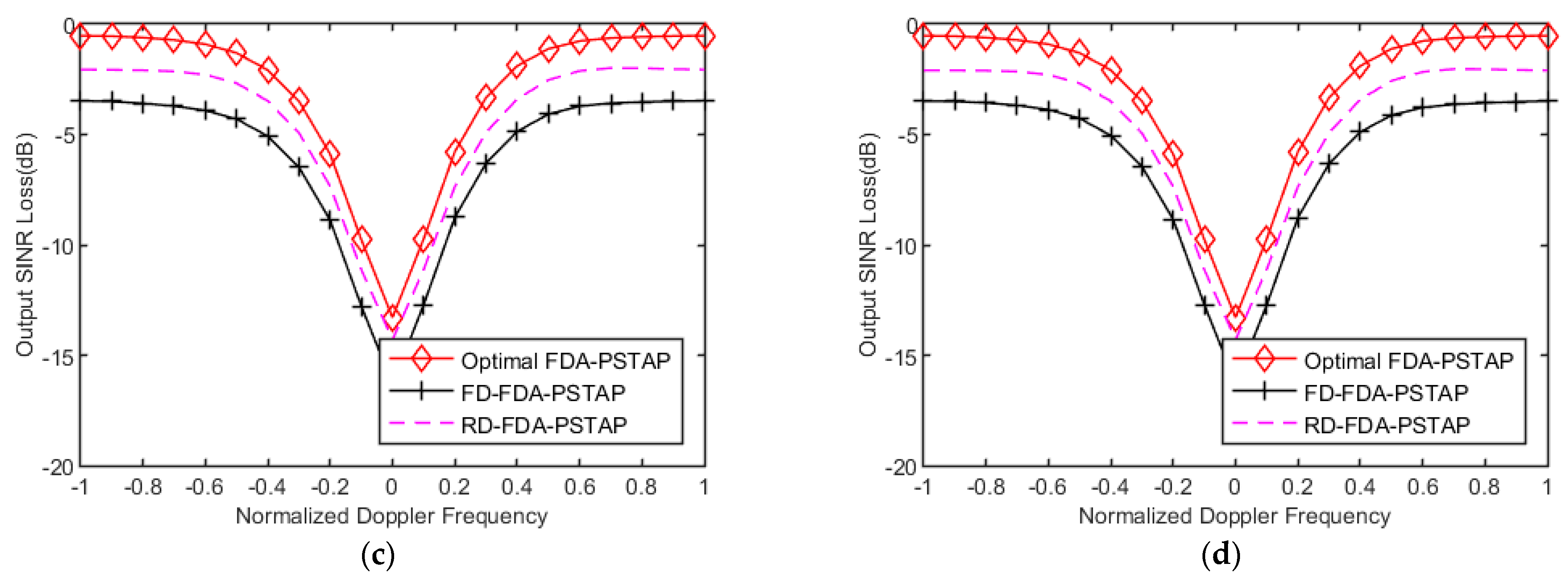
Figure 3 shows the SINR loss curves when the platform speed is increased to $V=300\mathrm{m}/\mathrm{s}$ and target polarization $\left({\gamma }_0,{\eta }_0\right)=\left(45°,65°\right)$. Raising the velocity from $150\mathrm{m}/\mathrm{s}$ to $300\mathrm{m}/\mathrm{s}$ doubles the slope of the clutter ridge in the angle-Doppler plane. As shown in Figure 3a, the performance of FD-FDA-PSTAP degrades significantly under $D=MNKP$. Its SINR loss exceeds 20 dB near the Doppler center and remains above 15 dB over a broad Doppler range. A larger clutter rank requires extra degrees of freedom for clutter cancelation; however, limited training samples prevent accurate estimation of the high-dimensional clutter subspace. In comparison, the proposed RD-FDA-PSTAP keeps the SINR loss around 10–15 dB in the main clutter region, achieving an SINR loss 13–15 dB lower than that of FD-FDA-PSTAP. In Figure 3b, FD-FDA-PSTAP achieves apparent performance improvement, with SINR loss reduced by about 1–2 dB compared with the $D=MNKP$ case. Nevertheless, it still lags behind RD-FDA-PSTAP by 2–3 dB around the clutter notch. Benefiting from improved covariance estimation with additional training samples, RD-FDA-PSTAP achieves SINR loss within 1–2 dB of the theoretical optimum across the whole Doppler range. These results verify the robustness of RD-FDA-PSTAP against the increased clutter rank induced by high platform velocity, which renders it suitable for high-speed airborne radar systems operating in complex clutter environments.

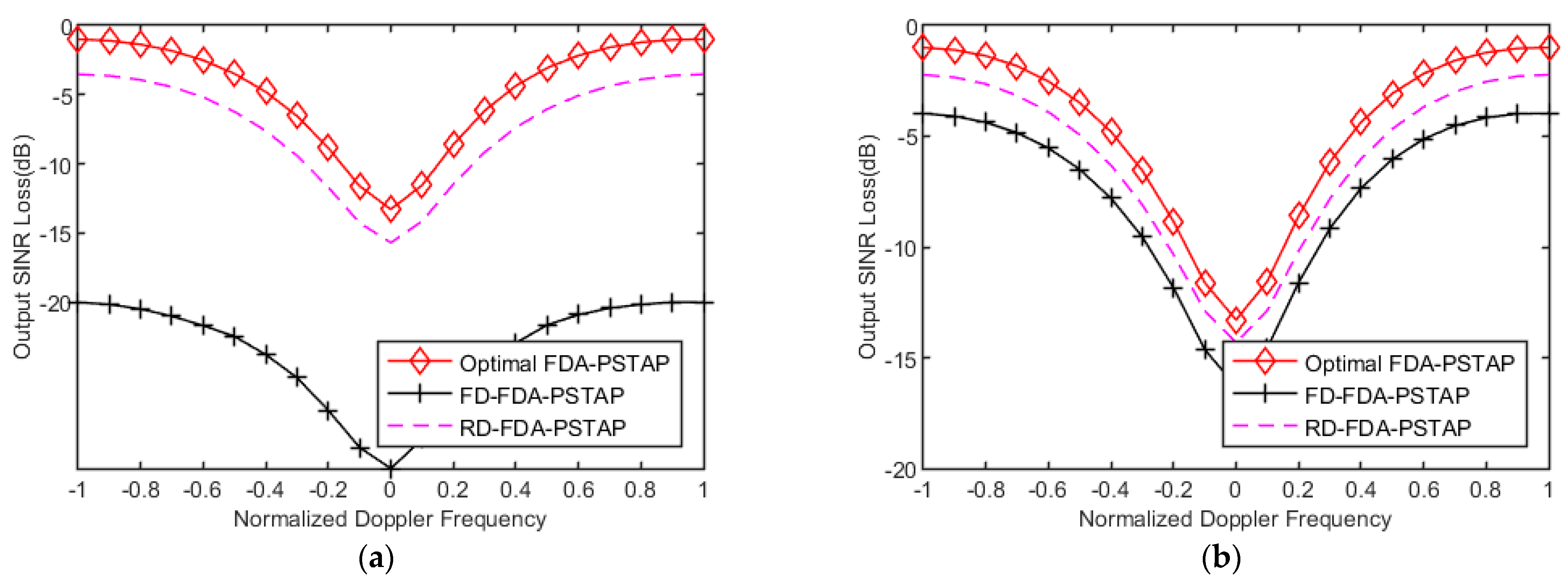
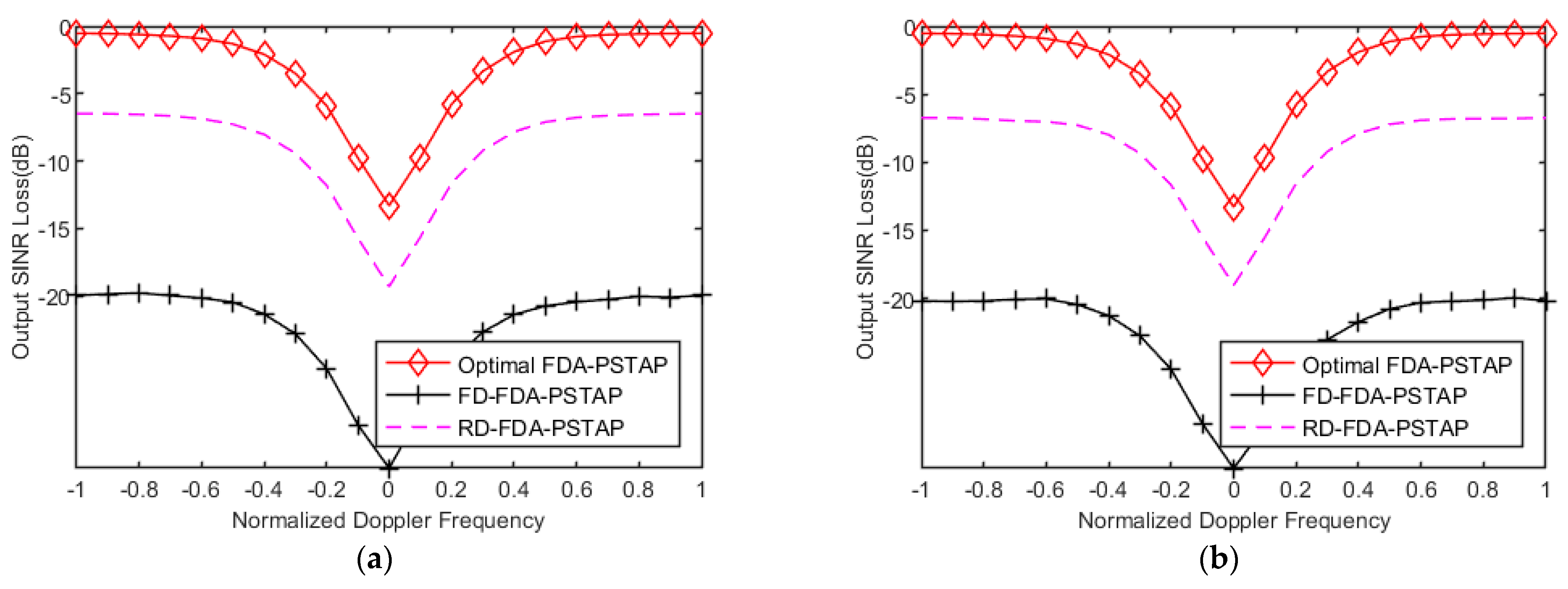
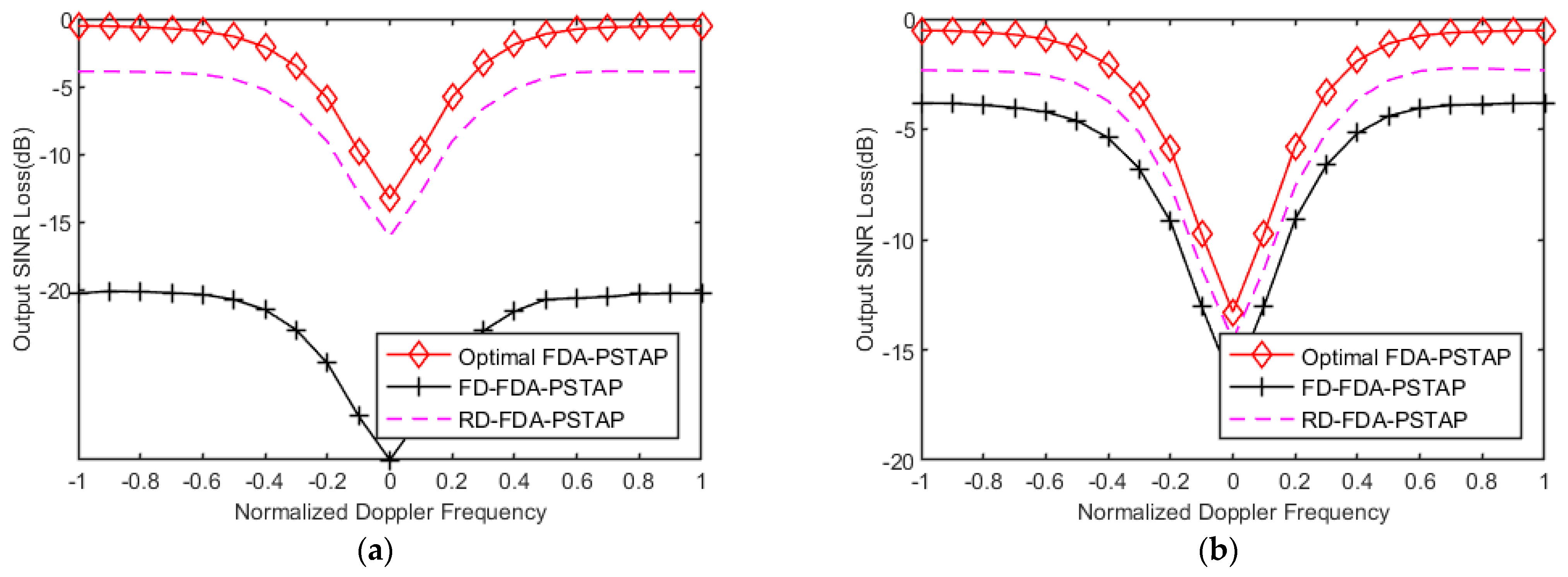
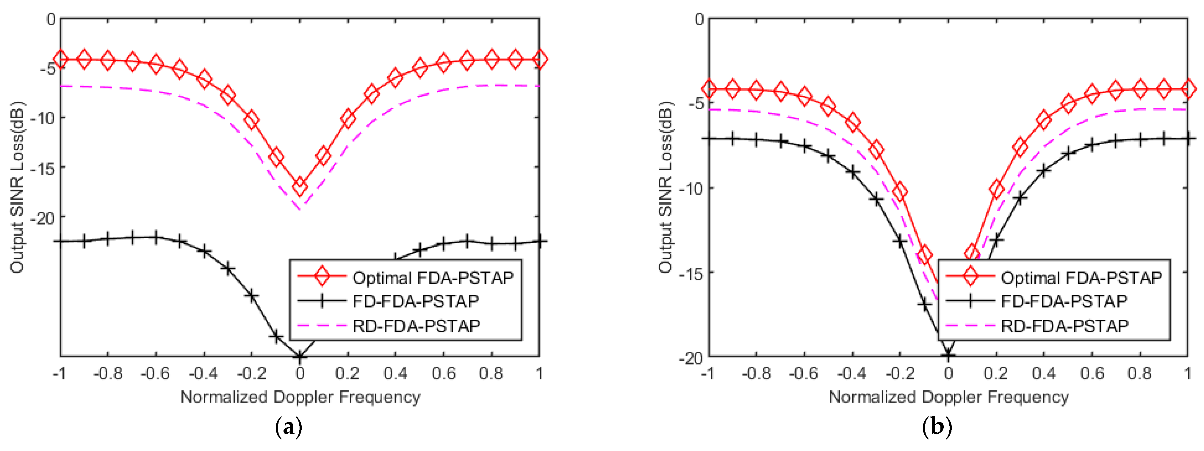
Figure 4 plots output SINR loss at $V=150\mathrm{m}/\mathrm{s}$ with target polarization set to $\left({\gamma }_0,{\eta }_0\right)=\left(20°,90°\right)$. Under the $D=MNKP$ condition, as shown in Figure 4a, the SINR loss of FD-FDA-PSTAP reaches nearly 20 dB around the clutter ridge, 2–3 dB higher than in Figure 3a. In contrast, RD-FDA-PSTAP maintains prominent superiority: its SINR loss is 5–7 dB lower within the main clutter region and 3–4 dB lower elsewhere. In Figure 4b, as the number of training samples is increased to $D=2MNKP$, both algorithms achieve appreciable performance gains. FD-FDA-PSTAP reduces its SINR loss by roughly 4–5 dB and narrows the performance gap. The proposed RD-FDA-PSTAP achieves lower SINR loss than FD-FDA-PSTAP across the entire Doppler spectrum. This result demonstrates the complementarity between space–time and polarization domains. Polarimetric processing alone cannot distinguish targets from clutter with similar polarization states, while the efficient space–time processing of RD-FDA-PSTAP compensates via angle-Doppler differences and sustains favorable clutter suppression performance.

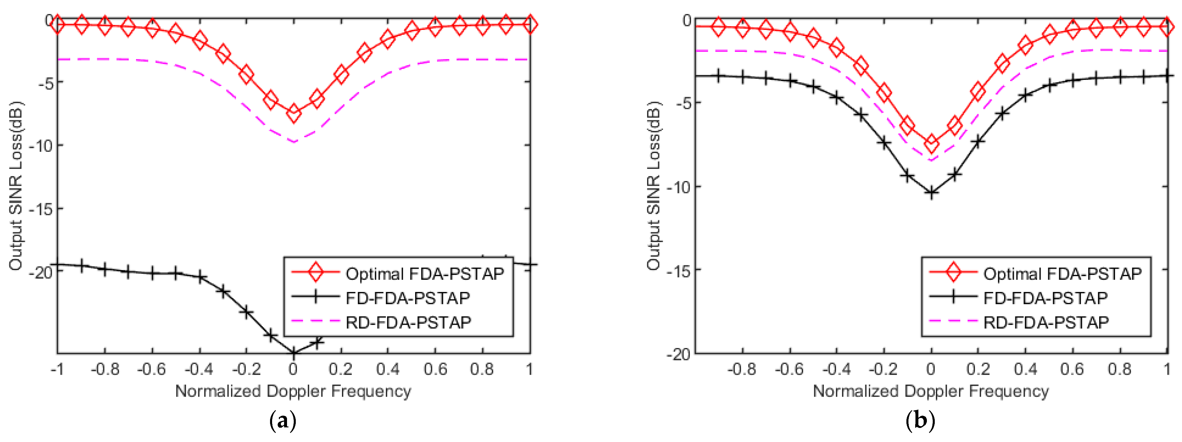
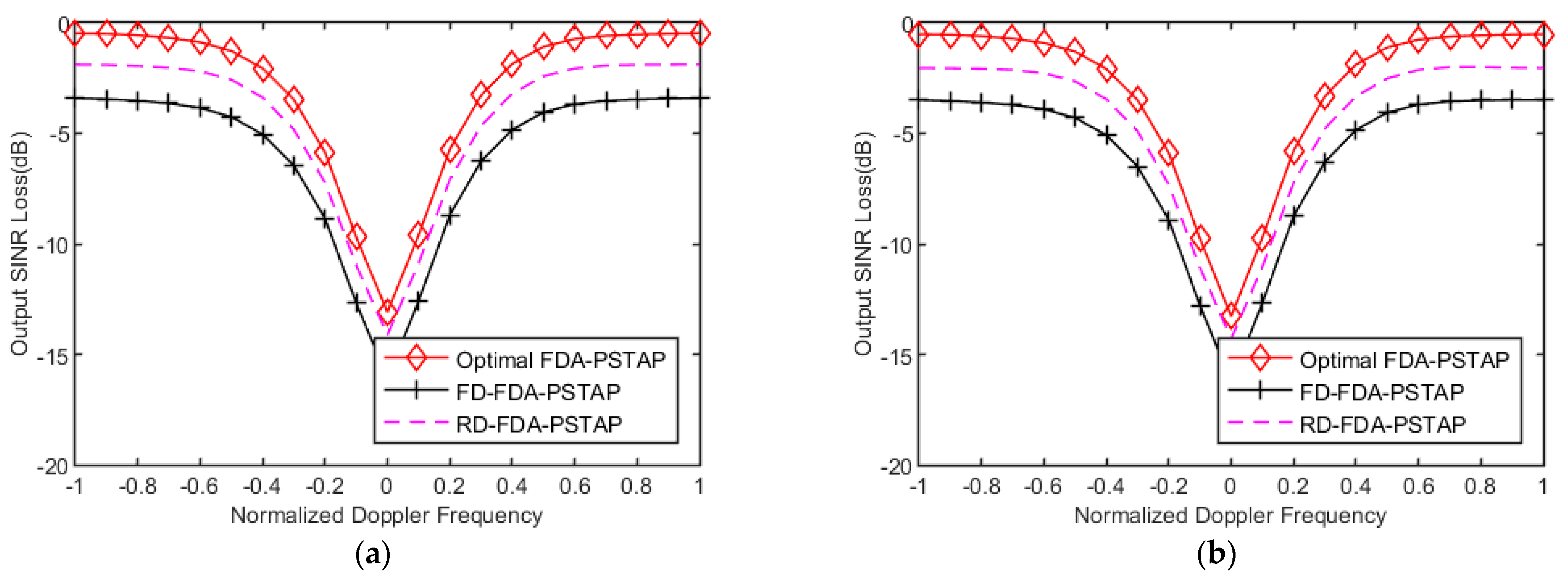
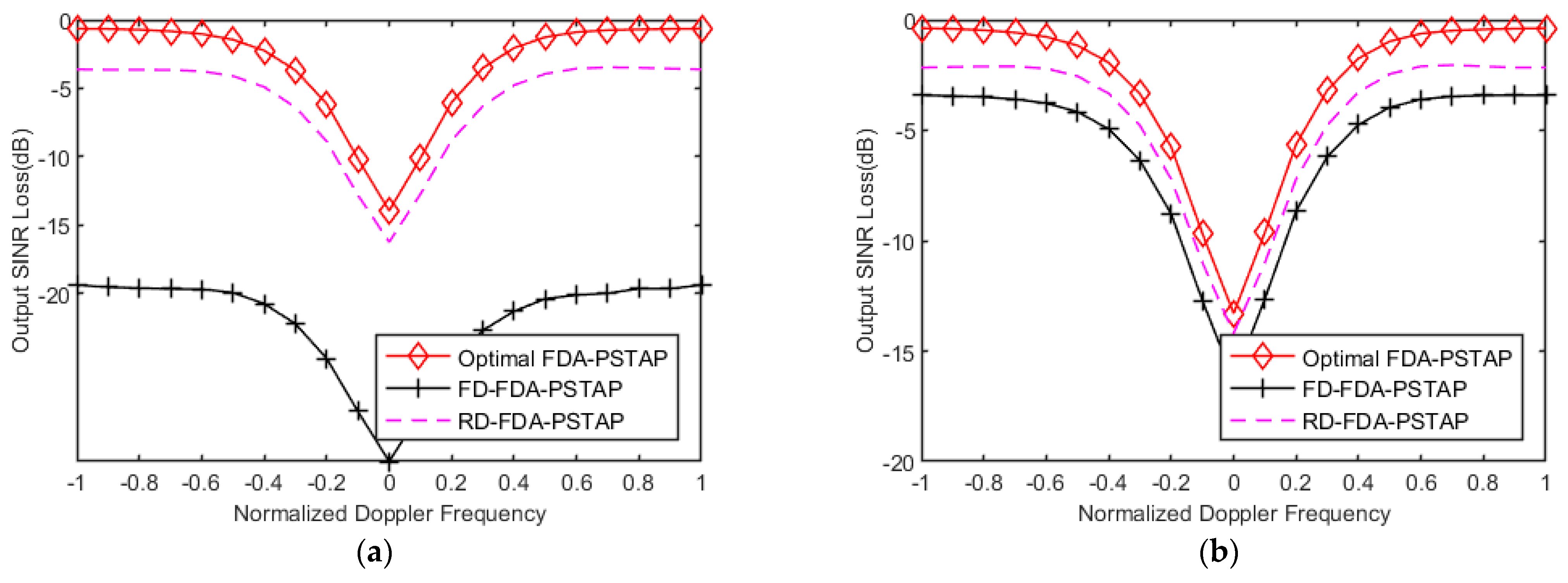
In Figure 5, the target polarization is set to $\left({\gamma }_0,{\eta }_0\right)=\left(20°,90°\right)$ and the platform speed is increased to $V=300\mathrm{m}/\mathrm{s}$. Under the $D=MNKP$ scenario, as shown in Figure 5a, FD-FDA-PSTAP suffers drastic performance degradation. Its SINR loss exceeds 20 dB around the Doppler center and stays above 18 dB over a wide Doppler range. By contrast, RD-FDA-PSTAP projects data onto a localized subspace, retaining only effective transmit, receive, and Doppler beams, which greatly reduces the effective dimensionality. Consequently, its SINR loss is 7–9 dB within the main clutter zone, approximately 14–16 dB lower than FD-FDA-PSTAP. When the number of training samples is increased to $D=2MNKP$, FD-FDA-PSTAP achieves a 5–7 dB reduction in SINR loss, as shown in Figure 5b. However, it still underperforms RD-FDA-PSTAP by approximately 2–3 dB near the clutter notch. Benefiting from improved covariance estimation, the proposed algorithm approaches optimal performance within a 1–2 dB SINR loss margin. Overall, the proposed RD-FDA-PSTAP maintains strong robustness and favorable clutter suppression even under the extreme condition of high speed plus poor polarization, which renders it highly applicable to practical airborne radar systems facing complicated working environments.

Figure 6 plots the output SINR losses versus normalized Doppler frequency under two different non-uniform reduced-dimensional parameter configurations $J_1\times J_2\times J_3=3\times 4\times 4$ and $J_1\times J_2\times J_3=4\times 3\times 4$, with $V=150\mathrm{m}/\mathrm{s}$, $\left({\gamma }_0,{\eta }_0\right)=\left(45°,65°\right)$, and $D=MNKP$. As shown in Figure 6, both non-uniform configurations of RD-FDA-PSTAP exhibit noticeable performance degradation near zero Doppler, with the maximum SINR loss reaching 19 dB. In contrast, the uniform $J_1\times J_2\times J_3=3\times 3\times 3$ configuration in Figure 2a reaches a maximum SINR loss of about 14 dB, achieving about 5 dB lower SINR loss. This indicates that uneven allocation of the reduced-dimensional parameters across dimensions increases the total degrees of freedom, degrading the covariance matrix estimation accuracy under limited training samples and thus impairing practical performance. By contrast, the uniform $J_1\times J_2\times J_3=3\times 3\times 3$ configuration satisfies the RMB criterion while achieving superior practical performance.

To further validate the robustness of the proposed RD-FDA-PSTAP, we provide additional simulation results for three and four range-ambiguity regions. Figure 7 plots the output SINR loss against the normalized Doppler frequency under the conditions $V=150\mathrm{m}/\mathrm{s}$, $\left({\gamma }_0,{\eta }_0\right)=\left(45°,65°\right)$, and $D=2MNKP$. As shown in Figure 7a,b, the proposed RD-FDA-PSTAP consistently achieves near-optimal performance across the entire Doppler spectrum, while the FD-FDA-PSTAP suffers from severe performance degradation due to insufficient training samples. These results confirm that the proposed method maintains effective clutter suppression regardless of the number of ambiguous regions, further demonstrating its robustness and practical applicability.

To examine the sensitivity of the proposed method to the clutter-to-noise ratio (CNR), we conducted additional simulations with $CNR=10\mathrm{dB}$, $20\mathrm{dB}$, $40\mathrm{dB}$, and $50\mathrm{dB}$, covering a broad range of practical airborne radar operating conditions. Figure 8 presents the output SINR loss versus normalized Doppler frequency under these four CNR settings, with $V=150\mathrm{m}/\mathrm{s}$, $\left({\gamma }_0,{\eta }_0\right)=\left(45°,65°\right)$, $D=2MNKP$, and the number of ambiguity regions set to two. As shown in Figure 8a–d, the proposed RD-FDA-PSTAP consistently achieves near-optimal clutter suppression performance across all CNR levels, while the FD-FDA-PSTAP exhibits significant performance degradation under limited training samples regardless of the CNR. These results confirm that the proposed method is robust to CNR variations and maintains its performance advantage over the full-dimension approach across a wide range of clutter environments.

To evaluate the performance of the proposed method under more realistic conditions, we conduct additional experiments using an inhomogeneous clutter scenario modeled according to [38], which provides high-fidelity clutter data. Figure 9 presents the output SINR loss versus normalized Doppler frequency under inhomogeneous clutter, with simulation parameters $V=150\mathrm{m}/\mathrm{s}$ and $\left({\gamma }_0,{\eta }_0\right)=\left(45°,65°\right)$, and the number of training samples set to $D=MNKP$ and $D=2MNKP$, respectively. As shown in Figure 9a,b, under the inhomogeneous clutter setting, all methods exhibit increased SINR loss compared with the homogeneous case in Figure 2a,b. Nevertheless, the proposed RD-FDA-PSTAP consistently maintains a clear performance advantage over the FD-FDA-PSTAP under both snapshot configurations. These results confirm that the proposed method retains effective clutter suppression capability even when the homogeneous clutter assumption is violated.

In practice, the target polarization scattering matrix cannot be known perfectly and must be estimated from the received data. To examine the sensitivity of the proposed method to polarization estimation errors, we conduct additional experiments with mismatched polarization parameters under conditions $V=150\mathrm{m}/\mathrm{s}$ and $D=2MNKP$. The actual target polarization is set to $\left({\gamma }_0,{\eta }_0\right)=\left(45°,65°\right)$, while the processor adopts deviated assumed values $\left({\widehat{\gamma }}_0,{\widehat{\eta }}_0\right)$. Two polarization-mismatch configurations $\left({\widehat{\gamma }}_0,{\widehat{\eta }}_0\right)=\left(42°,65°\right)$ and $\left({\widehat{\gamma }}_0,{\widehat{\eta }}_0\right)=\left(45°,62°\right)$ are considered. As shown in Figure 10a, when $\left({\widehat{\gamma }}_0,{\widehat{\eta }}_0\right)=\left(42°,65°\right)$, the SINR loss of RD-FDA-PSTAP remains essentially consistent across the entire Doppler spectrum with its performance in the absence of polarization mismatch (Figure 2b). As shown in Figure 10b, when $\left({\widehat{\gamma }}_0,{\widehat{\eta }}_0\right)=\left(45°,62°\right)$, both methods exhibit similar performance. These results demonstrate that the proposed RD-FDA-PSTAP is insensitive to polarization mismatch and maintains robust clutter suppression performance under practical polarization estimation errors.

To evaluate the robustness of the proposed method against array imperfections, we introduce 5% gain and phase errors into the transmit and receive steering vectors, following the model established in [39]. Figure 11 presents the SINR loss under this error level, with simulation parameters $V=150\mathrm{m}/\mathrm{s}$, $\left({\gamma }_0,{\eta }_0\right)=\left(45°,65°\right)$, and the number of training samples set to $D=MNKP$ and $D=2MNKP$ in Figure 11a and Figure 11b, respectively. The results are averaged over 100 independent Monte Carlo trials. As shown in Figure 11a, under the limited sample condition $D=MNKP$, the FD-FDA-PSTAP suffers severe performance degradation due to insufficient training samples, with SINR loss exceeding 20 dB in the main clutter region. In contrast, the proposed RD-FDA-PSTAP achieves approximately 15 dB SINR loss at zero-Doppler, demonstrating a clear advantage over the full-dimensional approach. Compared with the no-error case in Figure 2a, the performance of all three methods under 5% gain and phase errors remains almost unchanged, confirming that the considered error level does not noticeably affect the clutter suppression capability. When the number of training samples is increased to $D=2MNKP$ (Figure 11b), both sample-based methods benefit from improved covariance estimation accuracy. Compared with the no-error case in Figure 2b, the performance degradation caused by the 5% gain and phase errors is negligible. These results indicate that the proposed RD-FDA-PSTAP maintains robust clutter suppression performance under gain and phase errors.

Figure 12 presents the output SINR loss versus normalized Doppler frequency for the proposed Optimal FDA-PSTAP, FD-FDA-PSTAP, RD-FDA-PSTAP, and the extended RD-FDA-STAP of Ref. [31], under the conditions $V=150\mathrm{m}/\mathrm{s}$, $\left({\gamma }_0,{\eta }_0\right)=\left(45°,65°\right)$. Figure 12a and Figure 12b correspond to $D=MNKP$ and $D=2MNKP$, respectively. As shown in Figure 12a, under the limited sample condition $D=MNKP$, the extended RD-FDA-P-STAP of Ref. [31] exhibits severe performance degradation in the main clutter region around zero Doppler, with SINR loss reaching approximately 20 dB, which is comparable to that of the FD-FDA-PSTAP. In contrast, the proposed RD-FDA-PSTAP achieves a significantly lower SINR loss of about 15 dB in the same region, demonstrating a performance improvement of approximately 5 dB. This improvement is attributed to the additional polarimetric discrimination capability, which enables the proposed method to separate targets from clutter even when their space–time signatures overlap. When the number of training samples is doubled to $D=2MNKP$ in Figure 12b, both reduced-dimensional approaches benefit from improved covariance estimation accuracy. The performance gap between the extended RD-FDA-STAP of Ref. [31] and the proposed RD-FDA-PSTAP narrows to approximately 0.5–1 dB across the entire Doppler spectrum, confirming that the polarimetric extension provides robust and consistent performance gains regardless of the sample support.

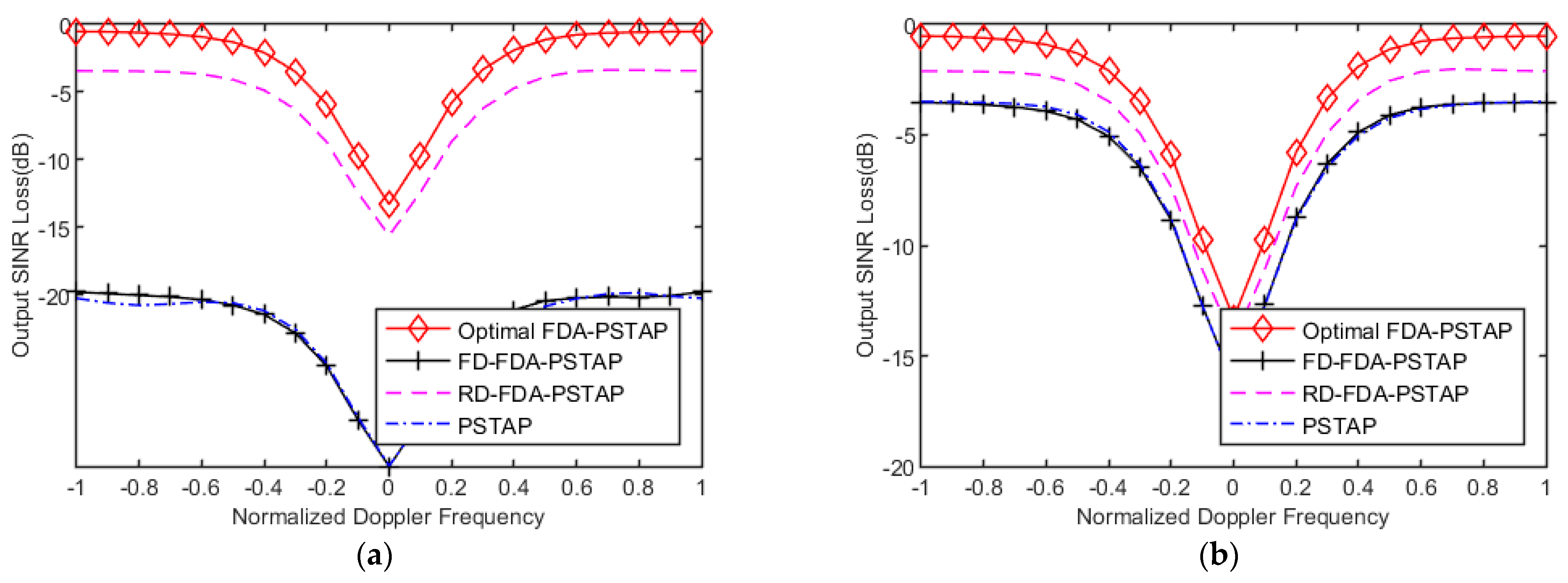
To provide a more comprehensive validation, we include ‘Conventional PSTAP without FDA’ as an additional baseline. Figure 13 presents the output SINR loss versus normalized Doppler frequency for the proposed Optimal FDA-PSTAP, FD-FDA-PSTAP, RD-FDA-PSTAP, and Conventional PSTAP without FDA, under the conditions $V=150\mathrm{m}/\mathrm{s}$, $\left({\gamma }_0,{\eta }_0\right)=\left(45°,65°\right)$. Figure 13a,b correspond to $D=MNKP$ and $D=2MNKP$, respectively. As shown in Figure 13a, the Conventional PSTAP without FDA exhibits severe performance degradation across the entire Doppler spectrum, with SINR loss exceeding 16 dB in the main clutter region around zero Doppler. This is because it lacks the range-dependent frequency diversity introduced by FDA, which makes it unable to separate clutter from different ambiguous range regions. In contrast, the proposed RD-FDA-PSTAP achieves significantly better performance, with SINR loss maintained at approximately 5–13 dB in the main clutter region, demonstrating the essential role of FDA in range-ambiguous clutter suppression. When the number of training samples is doubled to $D=2MNKP$ in Figure 13b, all FDA-based methods benefit from improved covariance estimation accuracy. The Conventional PSTAP without FDA also shows some performance improvement, yet it still lags substantially behind both FDA-based methods. These results confirm that the FDA technique is indispensable for effectively mitigating range-ambiguous clutter.

Figure 14 shows the output SINR losses under the mismatched condition, where all processors assume $q=1$ while the true target lies within $q=2$, with $V=150\mathrm{m}/\mathrm{s}$ and $\left({\gamma }_0,{\eta }_0\right)=\left(45°,65°\right)$. Subplots (a) and (b) correspond to $D=MNKP$ and $D=2MNKP$, respectively. To verify the range-ambiguous discrimination mechanism of FDA-PSTAP, we conduct a steering vector mismatch experiment. The transmit spatial frequency of FDA contains both angle-dependent and range-dependent terms. If the range term in the steering vector does not match the target’s true ambiguity region, the target signal cannot be properly matched. In this experiment, the true target is located in $q=2$, but all three processors erroneously use the steering vector of $q=1$ to construct their weights. As shown in Figure 14, under this mismatched condition, all processors exhibit a nearly flat SINR loss of approximately 5 dB across the entire Doppler spectrum, with the notch at the target Doppler being notably shallower than that observed in the matched case (Figure 2). This indicates that the target signal is largely suppressed as clutter, whereas under the matched condition, the target is properly preserved. This negative example confirms that FDA-PSTAP can effectively distinguish different range ambiguity regions through the range-dependent transmit spatial frequency.

6. Conclusions

In this paper, we introduce FDA into Conventional PSTAP to overcome range-ambiguous clutter and develop an FDA-PSTAP framework. First, we establish the fundamental signal model for polarimetric FDA radar, including signal transmission, signal reception, frequency mixing, matched filtering, and model approximation. Second, based on the MVDR criterion, we derive the full-dimensional FDA-PSTAP weight vector. Finally, to enhance the reliability of FDA-PSTAP under limited training samples, we design a localized transformation matrix to reduce the data dimension. According to the RMB rule, the developed reduced-dimensional FDA-PSTAP achieves a 15–17 dB improvement under limited training samples compared with the full-dimensional counterpart. Numerical results demonstrate that the proposed method achieves superior clutter suppression performance to the Conventional full-dimensional FDA-PSTAP and maintains its effectiveness across different target polarization states.