Evaluation and Prediction Methods for a Steel Company Using Six Sigma Metrics, Capability Indicators, and Markov Chains

Abstract

The operational dynamics of the steel industry constitute one of the work systems with the highest severity and accident rates. To address this, this research multidimensionally evaluates and stochastically predicts the preventive capability of the safety system in a steel plant. Using a quantitative, evaluative, and longitudinal three-phase design, the retrospective evaluation of nine preventive variables was employed using Six Sigma metrics (DPMO, $Z$, $Y$), along with the evaluation of overall performance through the Geometric Capability Indicator (GCI) and the Arithmetic Capability Indicator (ACI), and the stochastic modeling of the process using Markov chains. It was demonstrated that evaluating processes in isolation hides structural inefficiencies, as four variables showed an Excellent individual performance ($Z\approx 6.0$), but the comprehensive multivariate evaluation revealed a Deficient systemic state (GCI of 0.471 and ACI of 0.493). Furthermore, Markov modeling on the compliance of the process management index predicted a 100% probability of long-term stagnation in a deficient absorbing state ($x_1=1$). It is concluded that the proposed method functions as a rational anticipation system that provides potential managerial benefits by offering early warning indicators of operational degradation, supporting corrective decision-making on unstable preventive indicators.

1. Introduction

The operational dynamics of the steel industry configure one of the work systems with the highest severity and occupational accident rates [1,2,3]. Within this highly demanding manufacturing sector, processes present high internal variability due to constant interaction with heavy machinery, cutting tools, and high-temperature materials; conditions that increase the risk of operational failures and severe injuries [4,5,6]. Consequently, evaluating and controlling the capability of preventive safety management systems, rather than relying solely on reactive indicators or general production metrics, has become a vital necessity for modern steel organizations. To address this, the standardization of operational variability through proactive indicators (leading indicators) represents a crucial pathway toward operational excellence. From this perspective, the integration of Six Sigma metrics, multivariate capability indicators, and Markov chains provides a unified quantitative framework to standardize, aggregate, and stochastically project the preventive quality performance of the safety system over time.

Despite the demand for a comprehensive evaluation and simultaneous control of multiple processes in environments with high operational variability, organizational management has traditionally been based on static and qualitative univariate evaluations [7]. This conventional approach ignores that variability is an inherent characteristic of any system in real-world scenarios, which prevents clearly visualizing the true capabilities and limitations of the operation for proper evidence-based decision-making [1,6,8,9].

Faced with the limitations associated with qualitative methods, recent research has highlighted the relevance of adopting rigorous mathematical and control models to evaluate the real performance of safety systems [10,11]. In this sense, the integration of the Six Sigma methodology, through the calculation of defects per million opportunities (DPMO), the Sigma quality level (Z), and the yield (Y), has facilitated the standardization in measuring operational variability in various business sectors [12,13]. Likewise, by structuring these metrics with multivariate capability indicators, such as geometric and arithmetic ones, it has been possible to identify control deficiencies experienced by organizations when monitoring their risks in isolation or by basing their safety solely on the temporary absence of deviations that generate serious accidents [14,15]. Consequently, multivariate capability indicators have consolidated themselves as rigorous and novel instruments; their simultaneous application on various operational variables not only allows for the comprehensive evaluation and optimization of the system but also facilitates the detection of structural non-conformities and systemic weaknesses that, under traditional approaches, would remain hidden in operational management [12,16,17].

However, the comprehensive evaluation of industrial safety in steel companies still presents significant limitations in the control and monitoring of proactive and reactive indicators. As evidenced by recent literature focused on complex operational systems, there still persists a methodological disconnection between the conceptualization of safety standards, their practical measurement, and their control [18]. Thus far, quantitative methodologies have focused on the analysis of reactive indicators or variables associated with already materialized non-conformities, such as operational deviations, accidents that occurred, and lost time due to accidents. Although this analysis of past events is fundamental to understanding the historical variability of the management system, recent studies warn that the organizational dependence on these metrics is due to data availability; however, such tools lack predictive statistical capacity and hide systemic vulnerabilities under a false perception of control [18]. In this context, the accumulation of deviations in processes acts as the direct precursor to serious accidents. Therefore, with the purpose of mitigating the propagation of these events and guaranteeing operational performance and sustainability, it is necessary to establish an analytical process that transcends reactivity; that is, it is necessary to quantitatively measure the preventive capability of the system under diverse operational conditions [19].

In parallel, based on the premise that the consolidation of preventive quality does not follow a static behavior but presents fluctuations in response to the inherent variability of operations, this article introduces an innovative probabilistic dimension oriented toward the monitoring and management of risks in the industrial sector. In this context, the stochastic modeling of degradation and operational alterations has been established as a pillar within reliability engineering, demonstrating relevance in predictive diagnosis and asset life cycle management in manufacturing systems [20,21,22]. Despite these empirical advances, the adaptation of such principles to the specific environment of organizational safety implies a methodological disruption of rigorous analytical demand. Consequently, with the purpose of evaluating system behavior under changing operational scenarios, this research proposes the structuring of a longitudinal model through the application of Markov chains to estimate, under a probabilistic approach, the future transitions corresponding to the Sigma quality performance level (Z). In this way, this analytical convergence provides executive management with an objective anticipation instrument, grounded in rigorous statistical control, thereby allowing for the optimization of the prevention of non-conformities and safety events, and supporting the design of corporate strategies aimed at continuous improvement.

The motivation of this research is directed at designing a comprehensive statistical evaluation system that serves as a predictive and multidimensional diagnosis; a management control mechanism that overcomes the subjective or static nature of traditional tools to quantify the variability of operational performance against risk scenarios and serious events in the steel sector. Unlike previous literature, this proposal sequentially and complementarily combines the intensive use of Six Sigma metrics and multivariate statistical control to standardize preventive factors, integrating the mathematical modeling of Markov chains to stochastically predict the proactive capability of the operation. Contemporary research supports this approach by demonstrating that the transition toward a culture of preventive quality is inseparable from the incorporation of these predictive parameters [23]. Therefore, this structured approach constitutes an innovative contribution with highly replicable practical and continuous improvement implications in the global steel industry.

Previous scientific literature on safety management and process capability can be categorized into three main streams. The first stream focuses on reactive lagging indicators, which measure the outcomes of past accidents but lack predictive capacity to dynamically anticipate a system’s safety potential [24,25]. The second stream implements univariate Six Sigma quality metrics (such as DPMO, Z, and Y) to reduce process defects periodically, yet evaluates these dimensions in isolation, which risks ignoring functional correlations and masking overall system weaknesses [26,27,28]. The third stream explores multivariate capability indices (such as GCI and principal component analysis-based indicators) to globally assess multiple correlated characteristics or utilize probabilistic simulations and confidence intervals to model process capability under uncertainty [26,27,28,29]. To date, an integrated framework that sequentially combines these phases, using Six Sigma metrics to standardize individual dimensions, multivariate indicators to aggregate correlated variables, and probabilistic simulation or confidence intervals to stochastically project preventive quality, has not been fully developed or applied to safety-critical sectors and complex organizations [24,25,26,27,28]. This study addresses this gap, providing a novel and highly replicable anticipation instrument for proactive organizational management.

In this vein, to address the study problem and operationalize the analysis, the following research questions are posed: What is the appropriate procedure to establish a measurement and control system that allows for evaluating the performance of preventive safety indicators in a steel plant? How can Six Sigma metrics be used to quantitatively assess the individual performance of such preventive safety protocols? How can the comprehensive performance and maturation of the steel prevention system be evaluated through the application of geometric and arithmetic multidimensional capability indicators? Which of the three utilized criteria (Six Sigma metrics, geometric multidimensional capability indicator, and arithmetic multidimensional capability indicator) presents greater analytical rigor for detecting hidden non-conformities and guiding evidence-based managerial decision-making? How can the variations in Sigma yield levels (Z) be longitudinally modeled using Markov chains to determine the future transition probability in the maturity states of preventive quality for the variable with the highest variability in the steel system?

According to the questions raised above, the following specific objectives arise: (i) To characterize and define the preventive safety indicators that will make up the operational control and measurement system in the context of the steel plant. (ii) To evaluate the performance of the preventive safety protocols through the implementation of Six Sigma metrics (Defects per Million Opportunities DPMO, Sigma level Z, and yield Y). (iii) To evaluate the comprehensive performance and maturity of the operational safety system through the application of geometric and mean (arithmetic) multidimensional capability indicators. (iv) To conduct a comparative analysis between the performance of Six Sigma metrics and multidimensional capability indicators, to determine which criterion presents greater analytical rigor for the detection of non-conformities and managerial decision-making. (v) To predict, under a stochastic approach, the evolution of the variable with the highest variability in the plant’s safety system using a transition matrix based on Markov chains, grounded on the longitudinal monitoring of Sigma levels (Z).

2. Theoretical Framework

2.1. Quality in Preventive Management of the Steel Industry

In the environment of highly complex industrial operations, such as the steel sector, the occurrence of accidents is no longer considered a purely random phenomenon; on the contrary, contemporary literature defines them as the direct result of structural inefficiencies that progressively accumulate within the system [30,31]. To understand this dynamic holistically, current approaches rely on the loss control pyramid and the iceberg theory, demonstrating that materialized incidents are merely the visible section of process variability. Behind an adverse event, there lies an extensive base of latent deviations and non-conformities that silently deteriorate the quality of the work environment [32,33,34].

Despite the solidity of these theoretical foundations, the evaluation of industrial performance still operates under a strongly retrospective paradigm, limiting itself to monitoring through reactive metrics such as incident rates or lost time [8,9]. The core deficiency of these practices lies in analyzing the process in isolation after the materialization of the failure, which severely hinders the transition towards anticipatory models that guarantee standardized control [1,7]. Consequently, this reactive dependence allows uncontrolled variability to increase, compromising and violating the comprehensive stability of steel operations [35,36].

With the purpose of mitigating these systemic vulnerabilities, current demands require reorienting the evaluation towards the baseline conditions of the operating system through the design and statistical control of preventive indicators [30]. In contrast to traditional reactive metrics, these proactive instruments objectively quantify the state of the variables and the effectiveness of control actions in real time [9]. Applied to the steel sector, this methodological approach requires the quantitative evaluation of critical dimensions, such as the level of conformity in preventive reports, safety audits, maintenance programs, and strategies aimed at minimizing the behavioral variability of personnel [35,37].

Therefore, the articulated integration of these preventive parameters provides organizations with an indispensable capacity for early diagnosis and multidimensional quality evaluation [8]. Through longitudinal monitoring in early operational phases, executive management acquires the ability to evaluate the maturity level of the system and efficiently allocate resources towards improvement strategies based on empirical evidence [6,37]. From this perspective, the rigorous analytical monitoring of Leading Indicators is consolidated as the essential mechanism to neutralize the propagation of chain failures, interrupting the escalation of variability that transforms minor deviations into serious events and cementing an organizational culture rooted in preventive management [31,38].

2.2. Six Sigma Metrics

To control preventive indicators and manage the safety of the steel system, the Six Sigma methodology is consolidated as a strategic management tool aimed at the systematic mitigation of operational variability [16]. Integrating this philosophy aligns the performance of the protocols with the sustainable development of the system [39]. Therefore, when applied to industrial monitoring, it operates as a proactive instrument to identify, quantify, and neutralize deviations before they evolve into general non-conformities in the process [13].

To structure this evaluation, it is essential to define the operational parameters [40]: the total volume of evaluated units ($U$), where each monthly evaluation period represents one unit ($U=1$); the opportunities for error or non-conformity per evaluated unit ($O$), which corresponds to the maximum weighting or total compliance checkpoints established for each protocol; and the actual number of detected failures ($n$), calculated as the exact difference between the maximum opportunities ($O$) and the performance score actually achieved ($n=O-\mathrm{score}$) [41]. From this, the proportion of failures is calculated using the Defects per Million Opportunities (DPMO) indicator, which standardizes errors, facilitating the objective comparison between preventive protocols [42]. Its calculation obeys the formulation presented in Equation (1):

$$\mathrm{D}\mathrm{P}\mathrm{M}\mathrm{O}=\left({\displaystyle \frac{n}{U\times O}}\right)\times \mathrm{1,000,000}.$$

(1)

Subsequently, the Sigma quality performance level ($Z$) is determined, a central metric that translates the failure rate to a universal scale to quantify the degree of maturity and predictive capacity of the system under high-reliability conditions [41]. The results classify performance into standardized strata: Deficient ($Z<3.0$), Acceptable ($3.0\le Z<4.5$), and Excellent ($Z\ge 4.5$) [42]. As a final phase, the Yield ($Y$) is estimated, which illustrates operational efficiency by representing the percentage of tasks executed in strict compliance, free of deviations [12]. Their respective calculations are defined in Equations (2) and (3):

$$Z=\sqrt{29.3-2.221\times \ln \left(\mathrm{D}\mathrm{P}\mathrm{M}\mathrm{O}\right)}+0.8406,$$

(2)

$$Y=\left(1-{\displaystyle \frac{n}{\left(U\times O\right)}}\right).$$

(3)

In summary, the integration of these three metrics (DPMO, Z, and Y) constitutes a rigorous quantitative analytical framework that not only facilitates preventive monitoring and control but also supports decision-making aimed at operational excellence within the organization [43].

2.3. Multidimensional Capability Indicators

In the analysis of highly complex operating systems, the isolated evaluation of variables is statistically insufficient to understand the holistic performance of management. Due to the strict functional interdependence of the processes, contemporary literature requires integrating multiple control attributes into a single measurement vector that captures the real variability of the environment [16,44]. This multidimensional approach allows organizations to evaluate not only the quality of their individual processes but also the way in which they interact and integrate within the overall system [45]. Approaching reliability from this multivariate perspective empowers organizations not only to isolate specific non-conformities but also to diagnose how these deviations interact and compromise the global performance of the system [46,47], managing to normalize a set of individual indicators to aggregate them into a composite index [14].

To operationalize this integration, two rigorous mathematical approaches are implemented. In the first instance, the Geometric Capability Indicator (GCI) is established as the analytical criterion with the highest evaluative severity. This type of indicator, which aligns with the simultaneous monitoring of multiple characteristics under assumptions of normality and independence [48], allows for a robust analysis against various variability factors [15]. By being based on a model of multiplicative proportions, this indicator penalizes global performance if even a single preventive process manifests deficiencies [26]. This restrictive nature prevents isolated successes from masking structural weaknesses or latent non-conformities within the system. Its analytical formulation is expressed in Equation (4):

$$\mathrm{G}\mathrm{C}\mathrm{I}={\displaystyle \frac{1}{3}}{\mathsf{\Phi }}^{-1}{\left({\displaystyle \prod _{j=1}^v}{Y}_j\right)}^{{\displaystyle \frac{1}{v}}}+{\displaystyle \frac{1}{2}} ,$$

(4)

where ${\mathsf{\Phi }}^{-1}$ represents the inverse function of the cumulative standard normal distribution; $v$ corresponds to the total number of dimensions or preventive variables under evaluation in the system; and $Y_j$ constitutes the statistical yield obtained for dimension $j$.

In contrast, the Arithmetic Capability Indicator (ACI) operates as a central tendency model that softens the comprehensive assessment of the system. Supported by additive averages, this approach mitigates the negative impact generated by an isolated deviation, avoiding the collapse of the overall rating [12]. Consequently, it emerges as the ideal instrument for monitoring compensated general performance, providing a more flexible perspective of operational stability. This type of scheme facilitates an objective approach to decision-making, reducing the complexity of the problem through the joint analysis of data [49], and its calculation is given by Equation (5):

$$\mathrm{A}\mathrm{C}\mathrm{I}={\displaystyle \frac{1}{3}}{\mathsf{\Phi }}^{-1}\left[{\displaystyle \frac{\frac{{\displaystyle {\sum }_{j=1}^v}{Y}_j}{v}+1}{2}}\right],$$

(5)

where the term ${\displaystyle \frac{{\displaystyle {\sum }_{i=1}^v}{Y}_i}{v}}$ represents the arithmetic average yield of the dimensions subjected to evaluation.

Finally, to dictate operational reliability from these models, statistical control theory has unified three standardization thresholds. These series of capability evaluations allow estimating if the process reaches the defined tolerance limits [50]. The degree of systemic maturity is classified as Deficient if the index is strictly less than 0.50; it is assumed Acceptable (or under a stable state of control) if it fluctuates between 0.50 and 0.75; and it is consolidated as Excellent when exceeding the 0.75 threshold, mathematically certifying high reliability in the plant’s preventive operations [51].

Theoretical and Mathematical Properties of GCI and ACI

To validate the statistical soundness of GCI and ACI, we define their fundamental mathematical properties, supported by multivariate process capability literature:

• Standardized Mapping and Thresholds: While the individual yields ($Y_j$) are strictly bound to probability values between 0 and 1, the inverse cumulative standard normal distribution function ${\mathsf{\Phi }}^{-1}\left(p\right)$ maps these probabilities into a continuous variable on the real line [48,52]. This transformation allows the capability indicators to translate bounded success rates into a standardized continuous scale, enabling the establishment of rigorous operational thresholds (e.g., capability values $<0.50$ indicate a Deficient state, certifying objective operational boundaries) [26].
• Monotonicity: Both indicators are strictly monotonic. For any individual yield $Y_j$, the partial derivatives are strictly positive ($\partial \mathrm{GCI}/\partial Y_j>0$ and $\partial \mathrm{ACI}/\partial Y_j>0$). This ensures that any improvement in an individual preventive protocol mathematically increases the joint index [15].
• Sensibility and Rigor (AM-GM Inequality): By mathematical definition, the geometric mean of any non-negative set of numbers is always less than or equal to their arithmetic mean. Since ${\mathsf{\Phi }}^{-1}$ is a strictly increasing monotonic function, this relationship is preserved: $\mathrm{GCI}\le \mathrm{ACI}$. GCI acts as a highly sensitive indicator that penalizes the system if even one variable collapses, preventing isolated successes from masking critical failures [26,27].
• Independence and Robustness: While the GCI strictly assumes statistical independence among characteristics, real-world safety variables often exhibit functional correlation (e.g., dialog compliance and active participation). Under multicollinearity, the GCI acts as a conservative lower-bound estimate of the system’s capability, which represents an optimal, safety-first risk-management criterion [14,48].

2.4. Stochastic and Predictive Modeling Using Markov Chains

In the analysis of complex operating systems subject to constant operational variability, the stochastic modeling of temporal variability is addressed using Markov Chains, defined as discrete state-space stochastic processes characterized by the memoryless property (Markov property). Under this paradigm, the conditional probability distribution of future states depends exclusively on the present operational state [21], configuring a systemic approach that recognizes the synergy and interdependence of internal components with the purpose of optimizing the overall performance and productivity of the system [53]. By articulating this predictive perspective with quality management, the system states are directly linked to the Six Sigma performance levels ($Z$). This approach is fully consistent with the postulates of Multi-State System (MSS) theory, oriented toward evaluating the gradients of effectiveness or degradation of an industrial process [54,55].

Under this framework, operational performance is classified into standardized strata (Deficient if $Z<3.0$; Acceptable if $3.0\le Z<4.5$; and Excellent if $Z\ge 4.5$), quantitatively associating each stratum with the failure rate and the overall response capability of the operation. This continuous monitoring of probabilistic transitions provides an anticipated vision of quality, allowing the traditional and static statistical evaluation of Six Sigma to evolve into a predictive, longitudinal, and dynamic model. This transition facilitates the early identification of patterns, the preventive detection of bottlenecks, and the catalysis of continuous improvement [10], analytically integrating the behavior of variables under operational scenarios governed by volatility and constant variability [56,57].

To operate this dynamic, the transition probabilities between quality levels are structured into a one-step stochastic matrix ($P$), which mathematically illustrates the probabilistic rates of process fluctuation over time [20]. This matrix characterization is essential to rigorously simulate the behavior of interdependent subprocesses in highly changeable environments. Assuming that each column vector of the matrix constitutes an independent probability distribution whose sum is strictly equal to unity, and knowing the initial state vector ($x_0$), the fundamental equation of Markov processes makes it possible to analytically project the system towards any future instant $k$, facilitating a rigorous operational sensitivity analysis through the formulation presented in Equation (6):

$$x_k=P^k{x}_0.$$

(6)

This mathematical representation provides a dynamic and formal structure to the ex ante analysis, allowing for the anticipation of deviations from quality objectives and guiding strategic decision-making based on empirical evidence [11,58].

Beyond short-term projection, the strategic utility of this approach lies in its capacity to estimate the asymptotic convergence of the system after multiple operational cycles, a phenomenon that is quantified through steady-state probabilities [20]. From linear algebra, this operational equilibrium is defined by a stationary vector ($x$) that satisfies the stability condition $Px=x$, acting as an eigenvector of the transition matrix $P$ associated with the dominant eigenvalue $\lambda =1$. The analytical resolution of this state through the null space of the matrix ($P-I$) provides management with a rigorous mathematical instrument to comprehensively evaluate system stability under specific operational conditions [59]. In this way, it becomes feasible to predict whether the process will tend in the long term to stagnate in a deficient absorbing state (systemic degradation) or if it will reach levels of high reliability and operational maturity. Consequently, this modeling not only supports decision-making based on quantitative evidence and mitigates the occurrence of non-conforming outputs, but it also synergistically couples with advanced risk mitigation models and machine learning architectures [21,60].

3. Materials and Methods

This research was developed under a rational-positivist epistemological approach, adopting a quantitative, evaluative, and longitudinal design. In terms of its foundation, the work articulates empirical and factual research with a rational and proactive analytical model. Unlike traditional schemes oriented toward the retrospective or reactive evaluation of industrial safety, this study proposes a proactive and predictive analytical model, whose development is based on the collection and debugging of primary information extracted directly from the organization’s operational records to ensure maximum relevance and precision. This enables a strict, objective, and systematic numerical analysis of operational performance variability.

From this perspective of statistical control, the origin of science in this research is generated from the empirical comparison of the behavior of the preventive dimensions and variables, which allows objectively evidencing which statistical control criterion provides the diagnosis with the highest level of rigor for the industrial environment. For its part, the essence of science is based on the intensive use of metrics, indicators, and advanced statistical control tools to comprehensively evaluate, interpret, and monitor the system’s capabilities. Finally, as a criterion of truth, the comparative and longitudinal analysis of the results obtained from the application of Six Sigma metrics versus multidimensional indicators was established, contrasting them with the factual information of the operational process and validating the dynamic projection of performance through stochastic modeling. Data processing, Six Sigma capability calculations, and the Markovian stochastic modeling were performed using Microsoft Excel 365 (Microsoft Corporation, Redmond, WA, USA). Additionally, the methodological flowcharts and conceptual diagrams were created using the diagrams.net web application (draw.io Ltd, Northampton, UK; https://app.diagrams.net/, accessed on 20 July 2026).

As a basis for the development of the evaluation method,

Table 1. Nomenclature and abbreviations of the evaluated system.

Metric	Definition
$\mathrm{D}\mathrm{P}\mathrm{M}\mathrm{O}$	Defects per Million Opportunities
$Z$	Sigma quality performance level
$Y$	Process yield or effectiveness percentage
$U$	Total volume of evaluated units or evaluation frequency
$O$	Opportunities for errors per task or maximum weighting
$n$	Actual number of non-conformities or detected failures
GCI	Geometric Capability Indicator
ACI	Arithmetic (Mean) Capability Indicator
$v$	Total number of dimensions or variables under evaluation
$P$	Stochastic probability transition matrix
$x$	Markov Chain stationary vector
$E_1,{ E}_2,{ E}_3$	Quality performance states (Deficient, Acceptable, Excellent)
PSIF	Incidents with potential for serious injury or fatality
$V_1$	Compliance with daily safety dialogs
$V_2$	Participation in daily safety dialogs
$V_3$	Participation in safety hours
$V_4$	Completed actions from safety hours
$V_5$	Compliance with expected behavior audits
$V_6$	Compliance with the action plan for incidents that can cause serious injuries (PSIF)
$V_7$	Reporting of incidents with potential for serious injury or fatality by collaborators (PSIF)
$V_8$	Compliance with the closure of reported incidents
$V_9$	Compliance with the process management index

consolidates the general metrics, capability indicators, and preventive variables evaluated in the steel plant.

With the purpose of operationalizing the research design, ensuring rigor and traceability in data processing, and guaranteeing the systematic fulfillment of the outlined objectives, the empirical approach was structured through a three-phase sequential, complementary, and systemic method, which is analytically deployed through the following methodological steps:

• Phase 1: Evaluation of Preventive Performance Using Six Sigma Metrics

For the development of the analytical diagnosis, this initial phase was structured based on a longitudinal analysis that subjects the empirical frequency of non-conformities to statistical quality control equations. This procedure allows standardizing and quantifying the proportion of failures within the system. The operationalization of this first phase is carried out through the following five sequential steps, detailing the control objective expected to be achieved in each one:

Step 1: Collection and debugging of primary records. It consists of consolidating and cleaning the historical operational data of the steel plant.

Step 2: Delimitation of control variables. The 9 preventive parameters that regulate safety and risk management in the plant are conceptually defined.

Step 3: Operational parameterization of the system. The evaluated units ($U$), the latent opportunities for error ($O$), and the registered non-conformities ($n$) are formally determined.

Step 4: Normalization of defects using DPMO. The rate of defects per million opportunities is calculated for each variable through Equation (1).

Step 5: Determination of capability ($Z$) and yield ($Y$). The Sigma quality level and the effectiveness percentage of each preventive variable are calculated using Equation (2) and Equation (3), respectively.

• Phase 2: Comprehensive modeling using the multivariate capability indicator.

With the purpose of transcending the univariate and isolated evaluation of preventive processes, this phase seeks to model the interdependent and systemic behavior of safety in the steel plant. To this end, the individual yields ($Y$) obtained in the previous phase are assumed as proportions of mean operational success that interact jointly. Through a multivariate statistical control approach, two analytical capability models are applied complementarily, allowing the global and comprehensive evaluation of all system dimensions, triangulating their maturity degree against the standardization thresholds unified in the literature (Deficient, Acceptable/Good, and Excellent).

Step 6: Longitudinal yield processing. To ensure analytical clarity, the longitudinal dataset was processed under a dual-path approach: (1) Temporal Evaluation (Monthly), where the GCI and ACI were calculated for each of the 12 individual months using the joint performance of the 9 variables ($v=9$) in that specific period to observe time-series variation; and (2) Structural Evaluation (Annual), where the annual mean yield ($Y_j$) was calculated for each variable over the entire 12-month timeframe, and then aggregated into single GCI and ACI indices.

Step 7: Aggregation via Multivariate Indicators. The processed yields ($Y_j$) were mathematically aggregated utilizing the multi-attribute formulations established in Section 2.3. By applying the inverse cumulative standard normal distribution function (${\mathsf{\Phi }}^{-1}$) as defined in Equations (4) and (5), the joint performance of the system is synthesized to obtain the final systemic capability classifications in accordance with the established literature thresholds.

• Phase 3: Stochastic and Predictive Modeling Using Markov Chains for the Variable with the Highest Variability

This third phase aims to project what the long-term quality behavior of the system will be, based on the transition between its different historical performance states. To guarantee the viability and sharpness of the model, this discrete-time stochastic analysis is applied exclusively to the preventive variable that evidenced the highest variability and fluctuation in its quality levels during the evaluated cycle. This approach allows transitioning from a retrospective or static diagnosis to a preventive planning tool.

The operationalization of this predictive phase is carried out sequentially through the following methodological steps:

Step 8: Definition of quality performance states. It consists of classifying the historical Sigma quality level ($Z$) of the selected variable into three discrete, finite, and mutually exclusive states: Deficient ($Z<3.0$), Acceptable ($3.0\le Z<4.5$), and Excellent ($Z\ge 4.5$).

Step 9: Construction of the probability transition matrix ($P$). It consists of systematically recording and counting the monthly transitions experienced by the variable with the highest variability among the three defined states, structuring this information into a square matrix where it is algebraically verified that each column vector sums strictly to one.

Step 10: Steady-state modeling and calculation of the stationary vector. It consists of posing and analytically solving the Markovian stability matrix equation ($Px=x$), which acts as an eigenvector linked to the eigenvalue $\lambda =1$.

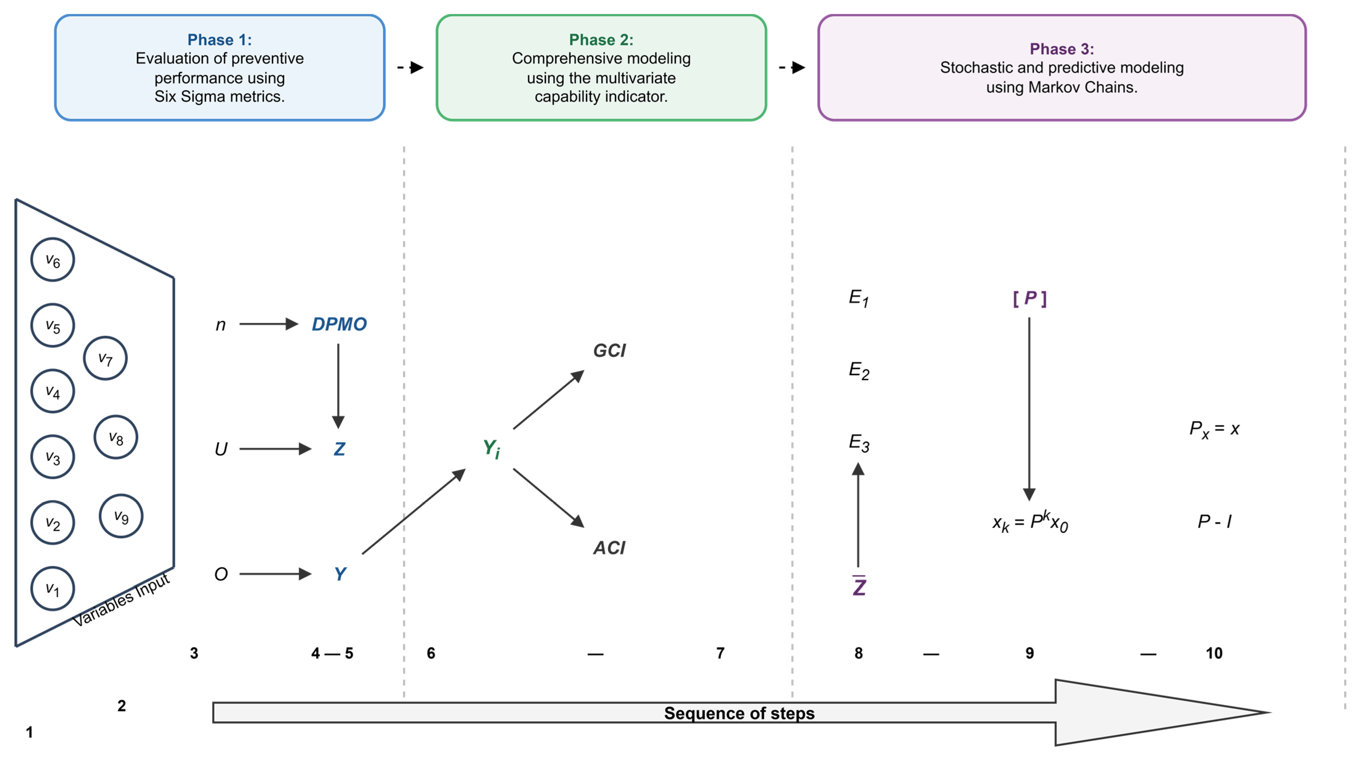
The holistic articulation of this three-phase method and its ten sequential steps is illustrated in detail in Figure 1. The consolidation of this methodological flowchart not only synthesizes the analytical convergence of the Six Sigma metrics, the multivariate indicators, and the Markov stochastic modeling, but it also constitutes a central contribution of the work by providing a structured, rigorous, and replicable methodology to sustainably evaluate and improve quality in any production or service environment.

4. Results

With the purpose of evaluating industrial safety performance in the steel sector and developing a comparative analysis among Six Sigma metrics, the geometric multidimensional capability indicator (GCI), and the arithmetic capability indicator (ACI), complemented by the forecast based on Markov chains, this research structured a longitudinal follow-up over twelve operational periods.

To operationalize this mathematical model, nine (9) preventive operational variables were identified and parameterized. These parameters form the core of the Verification Indicators system corresponding to the Leadership and Administration process of the steel plant. The characterization, the dimensions of analytical control, and the conceptual definitions of each of these preventive protocols are structured in detail in

Table 2. Operational parameterization and evaluation criteria for the system of preventive indicators.

Operational Variable	Maximum Weighting (O)	Operational Performance Intervals (%)	Assigned Score
Compliance with daily safety dialogs	5	0–54	0
		55–65	1
		66–75	2
		76–85	3
		86–99	4
		100	5
Participation in daily safety dialogs	5	0–89	0
		90–92	1
		93–95	2
		96–97	3
		98–99	4
		100	5
Participation in safety hours	10	0–59	0
		60–69	2
		70–79	4
		80–89	6
		90–95	8
		96–100	10
Completed actions from safety hours	10	0–49	0
		50–65	6
		66–75	7
		76–85	8
		86–95	9
		96–100	10
Compliance with expected behavior audits	15	0–49	0
		50–99	7
		100	15
Compliance with the action plan for incidents that can cause serious injuries (PSIF)	15	0–49	0
		50–65	3
		66–75	6
		76–85	9
		86–95	12
		96–100	15
Reporting of incidents with potential for serious injury or fatality by collaborators (PSIF)	15	0	0
		0.1–0.39	5
		0.4–0.69	10
		0.7–1.0	15
Compliance with the closure of reported incidents	15	0–49	0
		50–65	3
		66–75	6
		76–85	9
		86–95	12
		96–100	15
Compliance with the process management index	10	0–54	0
		55–65	6
		66–75	7
		76–85	8
		86–99	9
		100	10

and

Table 3. Characterization and scope of the preventive operational variables in the management system.

Evaluated Operational Variable	Characterization and Scope in Context
Compliance with daily safety dialogs	Evaluates the proportion of compliant execution of preventive dialog protocols implemented at the beginning of each operational cycle or work shift.
Participation in daily safety dialogs	Quantifies the rate of involvement and coverage of operational personnel in safety alignment spaces at the beginning of the workday.
Participation in safety hours	Measures the rate of adherence and participation of collaborators in the standardized practice of the safety hour within the steel environment.
Completed actions from safety hours	Determines the resolution effectiveness through the proportion of preventive actions satisfactorily executed and closed, relative to the total volume of pending deviations detected.
Compliance with expected behavior audits	Quantifies the degree of systematic execution of audits aimed at monitoring and controlling the behavioral variability of personnel in the plant.
Compliance with the action plan for incidents that can cause serious injuries (PSIF)	Evaluates the effective closure rate of corrective action plans derived from critical incidents, relative to the total volume of high-severity reports registered.
Reporting of incidents with potential for serious injury or fatality by collaborators (PSIF)	Monitors the rate of proactive reports issued by personnel regarding latent conditions or non-conformities that present high systemic risk or potential for fatality.
Compliance with the closure of reported incidents	Measures the efficiency rate in the resolution and formal closure of substandard events and operational deviations detected throughout the production process.
Compliance with the process management index	Quantifies the degree of maturity and the level of comprehensive achievement of the strategic management indicators previously parameterized for the control of the operational process.

, constituting the fundamental input for the execution of the first evaluation phase.

As evidenced in Table 2, the design of the evaluation system assigns a relative weight to each of the nine operational variables based on their criticality for industrial safety. It is highlighted that the factors with the highest maximum weighting (15 points each) are directly linked to the supervision and mitigation of critical risks, such as behavioral audits, the management and reporting of incidents with the potential for serious injuries (PSIF), and the effective closure of reported incidents. On the other hand, the tiered structuring of performance intervals allows preventive leadership and administration activities to be transformed into precise quantitative data. This rigorous parameterization ensures the standardization and objectivity of the measurements, guaranteeing that the input data are robust for the subsequent application of the Six Sigma metrics in the first phase of the analysis.

Table 3 provides evidence that these nine variables have a preventive focus, prioritizing the effective resolution of actions and the mitigation of critical risks (PSIF). Their standardized definition guarantees the reliability of the data that will feed the statistical models in the subsequent phases of the study.

• Phase 1: Preventive Performance Outcomes using Six Sigma Metrics

Information related to the nine variables has been collected over a 12-month period in the steel plant’s safety system. The results obtained for the analysis are presented in

Table 4. Results of the operational variables of the preventive system.

Evaluated Period	${\mathit{V}}_1$	${\mathit{V}}_2$	${\mathit{V}}_3$	${\mathit{V}}_4$	${\mathit{V}}_5$	${\mathit{V}}_6$	${\mathit{V}}_7$	${\mathit{V}}_8$	${\mathit{V}}_9$
January	5	1	8	10	15	12	15	12	10
February	5	2	10	9	15	12	15	12	10
March	5	2	10	9	15	9	15	3	10
April	5	2	10	9	15	12	15	12	9
May	5	2	10	9	15	9	15	9	9
June	5	2	10	9	15	9	15	9	9
July	5	3	10	9	15	12	15	12	9
August	5	2	10	9	15	12	15	12	8
September	5	4	10	9	15	12	15	12	9
October	5	4	10	9	15	12	15	12	9
November	5	4	10	9	15	15	15	12	8
December	5	2	10	8	15	9	15	12	8

Nomenclature of the evaluated variables: $V_1$: Compliance with daily safety dialogs. $V_2$: Participation in daily safety dialogs. $V_3$: Participation in safety hours. $V_4$: Completed actions from safety hours. $V_5$: Compliance with expected behavior audits. $V_6$: Compliance with the action plan for incidents that can cause serious injuries (PSIF). $V_7$: Reporting of incidents with potential for serious injury or fatality by collaborators (PSIF). $V_8$: Compliance with the closure of reported incidents. $V_9$: Compliance with the process management index.

.

With the information from Table 4, the variables were contextualized with the company’s primary information into Six Sigma metrics to evaluate the safety system under study.

• $U$: Number of the evaluation frequency of the indicator in the analyzed period.
• $O$: The value of the maximum weighting or ideal score established for each indicator, representing the total amount of units or evaluated points in which the system has the possibility to fail.
• $n$: Quantified empirically as the exact difference between said maximum opportunity ($O$) and the performance score achieved by the system in the period.
• $Y$: Variable yield.
• $\mathrm{D}\mathrm{P}\mathrm{M}\mathrm{O}$: Defects per million opportunities.

In this way, the calculation of the Six Sigma metrics is presented using Equations (1)–(3), through which the results of the defects per million opportunities ($\mathrm{D}\mathrm{P}\mathrm{M}\mathrm{O}$), the Sigma level value ($Z$), and the yield ($Y$) are obtained. The individual valuations are shown in

Table 5. Assessment of Six Sigma metrics for the safety system.

Variables	Period	$\mathit{O}$	$\mathit{U}$	$\mathit{n}$	$\mathbf{D}\mathbf{P}\mathbf{M}\mathbf{O}$	$\mathit{Z}$	$\mathit{Y}$
Compliance with daily safety dialogs	January	5	1	0	3.4	5.9964	100%
	February	5	1	0	3.4	5.9964	100%
	March	5	1	0	3.4	5.9964	100%
	April	5	1	0	3.4	5.9964	100%
	May	5	1	0	3.4	5.9964	100%
	June	5	1	0	3.4	5.9964	100%
	July	5	1	0	3.4	5.9964	100%
	August	5	1	0	3.4	5.9964	100%
	September	5	1	0	3.4	5.9964	100%
	October	5	1	0	3.4	5.9964	100%
	November	5	1	0	3.4	5.9964	100%
	December	5	1	0	3.4	5.9964	100%
Participation in daily safety dialogs	January	5	1	4	800,000	0.6600	20%
	February	5	1	3	600,000	1.2500	40%
	March	5	1	3	600,000	1.2500	40%
	April	5	1	3	600,000	1.2500	40%
	May	5	1	3	600,000	1.2500	40%
	June	5	1	3	600,000	1.2500	40%
	July	5	1	2	400,000	1.6473	60%
	August	5	1	3	600,000	1.2500	40%
	September	5	1	1	200,000	2.3206	80%
	October	5	1	1	200,000	2.3206	80%
	November	5	1	1	200,000	2.3206	80%
	December	5	1	3	600,000	1.2500	40%
Participation in safety hours	January	10	1	2	200,000	2.3206	80%
	February	10	1	0	3.4	5.9964	100%
	March	10	1	0	3.4	5.9964	100%
	April	10	1	0	3.4	5.9964	100%
	May	10	1	0	3.4	5.9964	100%
	June	10	1	0	3.4	5.9964	100%
	July	10	1	0	3.4	5.9964	100%
	August	10	1	0	3.4	5.9964	100%
	September	10	1	0	3.4	5.9964	100%
	October	10	1	0	3.4	5.9964	100%
	November	10	1	0	3.4	5.9964	100%
	December	10	1	0	3.4	5.9964	100%
Completed actions from safety hours	January	10	1	0	3.4	5.9964	100%
	February	10	1	1	100,000	2.7719	90%
	March	10	1	1	100,000	2.7719	90%
	April	10	1	1	100,000	2.7719	90%
	May	10	1	1	100,000	2.7719	90%
	June	10	1	1	100,000	2.7719	90%
	July	10	1	1	100,000	2.7719	90%
	August	10	1	1	100,000	2.7719	90%
	September	10	1	1	100,000	2.7719	90%
	October	10	1	1	100,000	2.7719	90%
	November	10	1	1	100,000	2.7719	90%
	December	10	1	2	200,000	2.3206	80%
Compliance with expected behavior audits	January	15	1	0	3.4	5.9964	100%
	February	15	1	0	3.4	5.9964	100%
	March	15	1	0	3.4	5.9964	100%
	April	15	1	0	3.4	5.9964	100%
	May	15	1	0	3.4	5.9964	100%
	June	15	1	0	3.4	5.9964	100%
	July	15	1	0	3.4	5.9964	100%
	August	15	1	0	3.4	5.9964	100%
	September	15	1	0	3.4	5.9964	100%
	October	15	1	0	3.4	5.9964	100%
	November	15	1	0	3.4	5.9964	100%
	December	15	1	0	3.4	5.9964	100%
Compliance with the action plan for incidents that can cause serious injuries (PSIF)	January	15	1	3	200,000	2.3206	80%
	February	15	1	3	200,000	2.3206	80%
	March	15	1	6	400,000	1.6473	60%
	April	15	1	3	200,000	2.3206	80%
	May	15	1	6	400,000	1.6473	60%
	June	15	1	6	400,000	1.6473	60%
	July	15	1	3	200,000	2.3206	80%
	August	15	1	3	200,000	2.3206	80%
	September	15	1	3	200,000	2.3206	80%
	October	15	1	3	200,000	2.3206	80%
	November	15	1	0	3.4	5.9964	100%
	December	15	1	6	400,000	1.6473	60%
Reporting of incidents with potential for serious injury or fatality by collaborators (PSIF)	January	15	1	0	3.4	5.9964	100%
	February	15	1	0	3.4	5.9964	100%
	March	15	1	0	3.4	5.9964	100%
	April	15	1	0	3.4	5.9964	100%
	May	15	1	0	3.4	5.9964	100%
	June	15	1	0	3.4	5.9964	100%
	July	15	1	0	3.4	5.9964	100%
	August	15	1	0	3.4	5.9964	100%
	September	15	1	0	3.4	5.9964	100%
	October	15	1	0	3.4	5.9964	100%
	November	15	1	0	3.4	5.9964	100%
	December	15	1	0	3.4	5.9964	100%
Compliance with the closure of reported incidents	January	15	1	3	200,000	2.3206	80%
	February	15	1	3	200,000	2.3206	80%
	March	15	1	12	800,000	0.6600	20%
	April	15	1	3	200,000	2.3206	80%
	May	15	1	6	400,000	1.6473	60%
	June	15	1	6	400,000	1.6473	60%
	July	15	1	3	200,000	2.3206	80%
	August	15	1	3	200,000	2.3206	80%
	September	15	1	3	200,000	2.3206	80%
	October	15	1	3	200,000	2.3206	80%
	November	15	1	3	200,000	2.3206	80%
	December	15	1	3	200,000	2.3206	80%
Compliance with the process management index	January	10	1	0	3.4	5.9964	100%
	February	10	1	0	3.4	5.9964	100%
	March	10	1	0	3.4	5.9964	100%
	April	10	1	1	100,000	2.7719	90%
	May	10	1	1	100,000	2.7719	90%
	June	10	1	1	100,000	2.7719	90%
	July	10	1	1	100,000	2.7719	90%
	August	10	1	2	200,000	2.7719	80%
	September	10	1	1	100,000	2.7719	90%
	October	10	1	1	100,000	2.7719	90%
	November	10	1	2	200,000	2.3206	80%
	December	10	1	2	200,000	2.3206	80%

, the mean yields per period are presented in

Table 6. Mean yields per period of the safety system.

Period	Mean DPMO	Mean Z	Mean Y
January	155,557.44	4.178	0.844
February	122,224.11	4.294	0.878
March	211,113.00	4.035	0.789
April	133,334.84	3.936	0.867
May	177,779.29	3.786	0.822
June	177,779.29	3.786	0.822
July	111,112.62	3.980	0.889
August	144,445.96	3.885	0.856
September	88,890.40	4.055	0.911
October	88,890.40	4.055	0.911
November	77,779.67	4.413	0.922
December	177,779.29	3.761	0.822

, and the annual mean yields per variable are found in

Table 7. Annual mean yields per variable of the safety system.

Evaluated Operational Variable	Mean DPMO	Mean Z	Mean Y
Compliance with daily safety dialogs	3.40	5.996	1.000
Participation in daily safety dialogs	500,000	1.502	0.500
Participation in safety hours	16,669.78	5.690	0.983
Completed actions from safety hours	100,000.28	3.003	0.900
Compliance with expected behavior audits	3.40	5.996	1.000
Compliance with the action plan for incidents that can cause serious injuries (PSIF)	250,000.28	2.402	0.750
Reporting of incidents with potential for serious injury or fatality by collaborators (PSIF)	3.40	5.996	1.000
Compliance with the closure of reported incidents	283,333.33	2.070	0.717
Compliance with the process management index	100,000.85	3.465	0.900

.

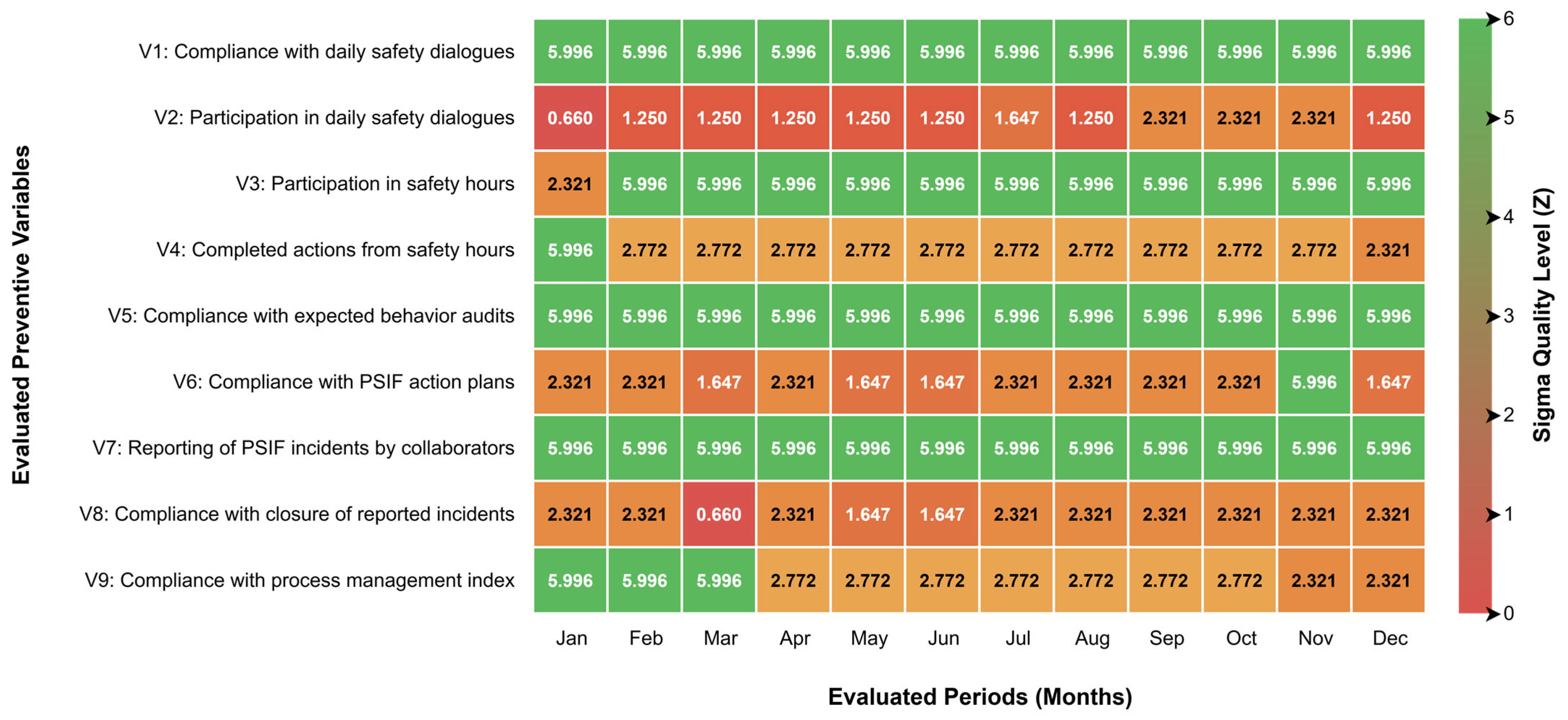
To complement the quantitative data compiled in Table 5 and facilitate its rapid systemic interpretation, a heatmap was developed to visually represent the temporal evolution of the monthly Sigma quality levels ($Z$) across all evaluated preventive dimensions, as shown in Figure 2.

Based on the results obtained in Table 6 regarding the assessment of the safety system variables using Six Sigma metrics, it can be affirmed that a sigma quality level in the acceptable range is evident, as all values fall within the range of $3.0\le Z<4.5$ in each period. However, a deficient performance is evident in all periods, presenting a yield ($Y$) of less than 95%.

Observing the results regarding the assessment of the operational variables of the steel plant’s safety system, it can be affirmed that four of the nine variables have an excellent sigma quality level and an excellent yield ($Y$) level. These variables are compliance with daily safety dialogs, participation in safety hours, compliance with expected behavior audits, and the reporting of incidents with potential for serious injury or fatality by collaborators (PSIF). On the other hand, there are two variables with a good sigma level: compliance with the process management index and completed actions from safety hours, although the latter borders the limits of becoming deficient. Furthermore, these two variables have a deficient yield. Finally, the remaining three variables exhibit deficient performance and yield.

• Phase 2: Systemic Capability Assessment via Multivariate Indicators

Considering Equation (4), the overall performance of the geometric multidimensional capability indicator of the safety process was evaluated, considering the 12 periods documented in Table 5 and the 9 variables from Table 6. In this case, $v=12$ months for the periods and $v=9$ for the variables; the data to be used are the mean yields ($Y$) of the 12 months, and the 9 variables are the $Y_i$ to apply the formulation:

$$\mathrm{G}\mathrm{C}\mathrm{I}={\displaystyle \frac{1}{3}}{\mathsf{\Phi }}^{-1} \left\{{\displaystyle \frac{{\left[0.844\times \dots \times 0.822\right]}^{1/12}+1}{2}}\right\}$$

$$\mathrm{G}\mathrm{C}\mathrm{I}={\displaystyle \frac{1}{3}}{\mathsf{\Phi }}^{-1}\left\{{\displaystyle \frac{0.8601+1}{2}}\right\}=0.492$$

It is evident that the overall performance of the geometric capability indicator evaluated by periods is 0.492. According to the measurement thresholds, the value is less than 0.50, which indicates the maturity of the steel system to be deficient.

Applying the same formulation to evaluate the variables ($v=9$):

$$\mathrm{G}\mathrm{C}\mathrm{I}={\displaystyle \frac{1}{3}}{\mathsf{\Phi }}^{-1} \left\{{\displaystyle \frac{{\left[1.0\times \dots \times 0.900\right]}^{1/9}+1}{2}}\right\}$$

$$\mathrm{G}\mathrm{C}\mathrm{I}={\displaystyle \frac{1}{3}}{\mathsf{\Phi }}^{-1}\left\{{\displaystyle \frac{0.8426+1}{2}}\right\}=0.471$$

When evaluating the capability of the safety process, it can be evidenced that it is in a deficient state, presenting a geometric capability indicator value lower than 0.5.

Now considering Equation (5), we proceed to evaluate the performance of the safety process using the mean multidimensional capability indicator, considering Table 5 and Table 6. This measurement is performed for the 12 evaluated periods; this section presents the following value:

$$\mathrm{A}\mathrm{C}\mathrm{I}={\displaystyle \frac{1}{3}}{\mathsf{\Phi }}^{-1}\left\{{\displaystyle \frac{\left[0.844+\cdots +0.822\right]/12+1}{2}}\right\}$$

$$\mathrm{A}\mathrm{C}\mathrm{I}={\displaystyle \frac{1}{3}}{\mathsf{\Phi }}^{-1}\left\{{\displaystyle \frac{0.8611+1}{2}}\right\}=0.493$$

Now we will apply the same equation, but evaluating the annual performance of the preventive variables ($v=9$):

$$ACI={\displaystyle \frac{1}{3}}{\mathsf{\Phi }}^{-1} \left\{{\displaystyle \frac{\left[1.00+\cdots +0.900\right]/9+1}{2}}\right\}$$

$$ACI={\displaystyle \frac{1}{3}}{\mathsf{\Phi }}^{-1} \left\{{\displaystyle \frac{0.8611+1}{2}}\right\}=0.493$$

The result of the arithmetic multivariate capability indicator in both cases was 0.493, and according to the measurement threshold, the value is below the 0.5 range; therefore, it can be affirmed that the prevention system is in a deficient state.

Now we will perform a comparative analysis of the performance of the Six Sigma metrics, the geometric quality capability indicator, and the mean capability indicator.

Based on the first five equations proposed in this research, the metrics and multidimensional capability indicators of the nine operational variables that constitute the safety system of the steel plant were calculated, as shown in

Table 8. Comparative analysis of Six Sigma metrics and multivariate capability indicators in the assessment of the safety system.

Evaluated Operational Variable	Mean DPMO	Mean Z	Mean Y	GCI	ACI
Compliance with daily safety dialogs	3.40	5.996	1.000	1.504	1.504
Participation in daily safety dialogs	500,000	1.502	0.500	0.225	0.225
Participation in safety hours	16,669.78	5.690	0.983	0.796	0.796
Completed actions from safety hours	100,000.28	3.003	0.900	0.548	0.548
Compliance with expected behavior audits	3.40	5.996	1.000	1.504	1.504
Compliance with the action plan for incidents that can cause serious injuries (PSIF)	250,000.28	2.402	0.750	0.383	0.383
Reporting of incidents with potential for serious injury or fatality by collaborators (PSIF)	3.40	5.996	1.000	1.504	1.504
Compliance with the closure of reported incidents	283,333.33	2.070	0.717	0.358	0.358
Compliance with the process management index	100,000.85	3.465	0.900	0.548	0.548

Note: It should be noted that, when evaluating each preventive variable individually ($v=1$), the results of the Geometric Capability Indicator and the Mean Multidimensional Indicator converge to the same mathematical value, because the geometric mean and the arithmetic mean of a single value collapse into the same figure.

.

From the results found in this research, the multivariate capability indicators, proposed as a tool for the comprehensive assessment of the steel safety system, have greater analytical rigor than traditional Six Sigma metrics such as $\mathrm{D}\mathrm{P}\mathrm{M}\mathrm{O}$, $Y$, $Z$, and $n$. This is because these multivariate indicators evaluate the interdependence of the processes and yield more conservative overall values, preventing the isolated performance of a single factor from distorting reality. The empirical evidence allows us to point out in this research that the most demanding criterion among those used is the geometric multidimensional capability indicator (GCI).

Furthermore, when evaluating the 9 variables transversally, it can be observed that while the Six Sigma metrics show an excellent performance in specific individual dimensions (for example, compliance with daily safety dialogs, participation in safety hours, compliance with expected behavior audits, and the reporting of incidents with potential for serious injury or fatality by collaborators (PSIF) present $Y$ yield levels of 100% and a $Z$ quality level close to 6.0), when analyzing the comprehensive performance of all dimensions of the prevention system using the mean multivariate capability indicator (ACI), it reaches an overall value of only 0.493, and the geometric multidimensional capability indicator (GCI) reaches an even lower value of 0.471.

This empirically demonstrates that the multidimensional geometric capability indicator (0.471) is more demanding than the mean capability indicator (0.493), and that, together, these multivariate instruments are notably more rigorous than the Six Sigma metrics used globally to improve processes. In this way, it is evidenced that the multivariate indicators reveal a deficient performance state, by presenting values lower than 0.50, which exposes the structural improvement opportunities and hidden non-conformities in the organization that, under a traditional measurement approach, would remain unaddressed in the plant’s management.

• Phase 3: Long-term Predictive Projections using Markov Chains

To ensure statistical rigor, the selection of the variable for the Markovian analysis was based on the standard deviation ($S{D}_Z$) of the monthly Sigma levels ($Z$) compiled in Table 5. While variables like $V_1$, $V_5$, and $V_7$ remained completely static ($S{D}_Z=0$), the variable $V_9$ (Compliance with the process management index) exhibited the highest operational instability and variability, showing a standard deviation of $S{D}_Z=1.344$ and a transition range of 3.67, dropping from an Excellent quality level ($Z=5.9964$ in January) to a Deficient level ($Z=2.3206$ in November) as documented in Table 5.

To model these dynamics stochastically, the performance levels of the process are classified into discrete quality states using the Six Sigma thresholds defined in

Table 9. Classification criteria for Markov states according to the Sigma Level ($Z$).

States	Nomenclature	Performance
State 1	E1—Deficient	Z < 3.0
State 2	E2—Good	3.0 ≤ Z < 4.5
State 3	E3—Excellent	Z ≥ 4.5

(State $E_1$—Deficient for $Z<3.0$; State $E_2$—Acceptable for $3.0\le Z<4.5$; and State $E_3$—Excellent for $Z\ge 4.5$).

Based on these criteria, the monthly sequence of operational states for $V_9$ was identified and mapped in

Table 10. Monthly temporal sequence of operational states.

Period	Z	States
January	5.9964	E3
February	5.9964	E3
March	5.9964	E3
April	2.7719	E1
May	2.7719	E1
June	2.7719	E1
July	2.7719	E1
August	2.3206	E1
September	2.7719	E1
October	2.7719	E1
November	2.3206	E1
December	2.3206	E1

.

With 12 monthly observation periods, a total of 11 sequential transitions were recorded for $V_9$ (Table 10). The empirical state frequencies were State $E_3$ (Excellent) = 3 months, State $E_2$ (Acceptable) = 0 months, and State $E_1$ (Deficient) = 9 months, as displayed in Table 10. The actual transition counts from one month to the next were: $E_3\to E_3$ = 2 times (January–February and February–March); $E_3\to E_1$ = 1 time (March–April); and $E_1\to E_1$ = 8 times (April–May, May–June, June–July, July–August, August–September, September–October, October–November, and November–December). All other transition frequencies were zero, which mathematically supports the transition probabilities used to construct the matrix $P$.

The temporal sequence reflects an operational collapse in the process: $E_3,{ E}_3,{ E}_3,{ E}_1,{ E}_1,{ E}_1,{ E}_1,{ E}_1,{ E}_1,{ E}_1,{ E}_1, E_1$. Now, the initial state vector $x_0$ defines how the process starts at time zero. In January, the $Z$ value was 5.9964, so the process begins with a 100% probability in State 3. Organized in the order $E_1,E_2,E_3$, the initial vector is defined as:

$$x_0=\left[\begin{array}{c}0\\ 0\\ 1\end{array}\right]$$

Considering the empirical transition probabilities calculated from the 11 observed monthly steps, the transition matrix $P$ is constructed:

$$P=\left[\begin{array}{ccc}1& 0& 0\\ 0& 1& 0\\ 1/3& 0& 2/3\end{array}\right]$$

To predict at what vulnerability level this variable will stagnate in the future, we must find the stationary vector $x$, which complies with $Px=x$. We calculate it by subtracting the identity matrix $I$ from our transition matrix $P$ and finding its null space:

$$P-I=\left[\begin{array}{ccc}1-1& 0& 0\\ 0& 1-1& 0\\ 1/3& 0& 2/3-1\end{array}\right]=\left[\begin{array}{ccc}0& 0& 0\\ 0& 0& 0\\ 1/3& 0& -1/3\end{array}\right]$$

Now, to set up the system of equations, this matrix is multiplied by the generic stationary vector ${\left[x_1,x_2,x_3\right]}^T$ and set equal to zero:

$$\mathrm{Row} 1: {\displaystyle \frac{1}{3}}{x}_3=0⟹x_3=0$$

$$\mathrm{Row} 3:-{\displaystyle \frac{1}{3}}{x}_3=0⟹x_3=0$$

It is evident that the probability of being in State 3 in the long term becomes zero ($x_3=0$). Since the variable started in $E_3$ and the transition matrix shows that there is no probability connecting $E_3$ or $E_1$ with State 2 (row 2 has zero probability from $E_1$ and $E_3$), it is impossible for the system to ever reach State 2 if no improvements are made in the process. Therefore, $x_2=0$. In this way, since the vector must sum to 1 ($x_1+x_2+x_3=1$), when substituting the zeros, we have that $x_1=1$. Thus, the final stationary vector is:

$$x=\left[\begin{array}{c}1\\ 0\\ 0\end{array}\right]$$

The stochastic modeling of the Compliance with the process management index variable reveals a critical managerial dynamic. Although the system started in an Excellent state ($Z>4.5$), the transition matrix $P$ evidenced a structural risk of falling (1/3) towards a Deficient state. The calculation of the stationary vector mathematically confirms the worst-case scenario: once the process falls to the Deficient level (State 1), it lacks the necessary recovery dynamics, becoming an absorbing state. In the long term, it is predicted with a 100% probability that the process will remain stagnant at a deficient quality level ($x_1=1$), unless management applies corrective interventions to the system.

Model Validation Against Real Operational Outcomes

The mathematical predictions of our integrated model were validated against the actual longitudinal records of the steel facility. The steady-state analysis predicted a 100% probability ($x_1=1$) of long-term stagnation in the Deficient state ($E_1$), classifying it as an absorbing state. This prediction is fully validated by the empirical data: following the operational collapse of variable $V_9$ in April, the process remained trapped in State for nine consecutive months (April to December) without showing any self-recovery dynamics. Furthermore, while traditional univariate approaches falsely suggested a highly capable safety system by focusing on individual Excellent variables ($V_1,V_5,V_7)$ (V, our joint multivariate GCI (0.471) successfully validated that the system was structurally deficient, identifying the exact precursor ($V_9$) that led to the operational stagnation.

5. Discussion

In fulfillment of the proposed objectives, this research proposed the multidimensional evaluation and stochastic prediction of the preventive capability of the safety system in a steel plant, through the integration of Six Sigma metrics (DPMO, Z, Y), multivariate capability indicators, and Markov chains. Other research also evaluated the performance and reduction in variability in the industrial sector using the Six Sigma methodology. Such is the case of Esmaili et al. [13] and Barreto and Herrera [12], who offer a strategic vision to standardize operational measurement and mitigate defects. However, unlike the current research, authors such as Orvik and Albrechtsen [18] and Sarmah and Dhalmahapatra [8] approach operational safety by basing decision-making on retrospective or qualitative tools, warning that dependence on purely reactive metrics lacks predictive capacity and hides systemic vulnerabilities.

Secondly, other authors in their research evaluated and measured the performance of operating systems supported by retrospective and qualitative tools. Orvik and Albrechtsen [18] and Sarmah and Dhalmahapatra [8] examined the impact of safety control, warning that dependence on reactive metrics lacks predictive capacity and hides systemic vulnerabilities. In contrast, this research used Six Sigma metrics and geometric (GCI) and arithmetic (ACI) controls to evaluate not only the service as a whole but each of the preventive indicators that compose it. It was empirically demonstrated that, although dimensions such as incident reporting (PSIF) present an Excellent quality level (Z ≈ 6.0), the interdependence of the process evaluated through the GCI reveals an overall Deficient state of 0.471.

On the other hand, the proposed research comprehensively implemented Six Sigma measurement tools articulated with the multivariate capability indicator (GCI and ACI) to evaluate the interdependent behavior of the steel system. In isolation, the system showed that specific preventive variables, such as compliance with daily dialogs and critical incident reports (PSIF), presented an Excellent individual performance, with yields (Y) of 100% and a Z quality level close to 6.0. Similar studies have also evaluated multidimensional control; for example, Casacci and Pareto [14] and Khadse and Shinde [15] developed evaluative approaches using multivariate capability indicators to identify control deficiencies. Despite this, in contrast to these investigations, the present study adopts an approach of evaluative severity, demonstrating that the interaction of these metrics, translated into a GCI of 0.471 and an ACI of 0.493, reveals a Deficient global systemic state. This offers a holistic evaluation that prevents isolated temporary successes from distorting the reality of the system.

Based on the results obtained, it was necessary to highlight the contribution of this study, which not only implements multivariate geometric rigor but also introduces a methodological disruption through stochastic modeling with Markov chains on the variable with the highest operational instability: Compliance with the management index. In comparison, although in the literature statistical control is used to determine system defects, the implementation and analysis of the probabilistic transition matrix ($P$) and the calculation of the stationary vector ($x$) provide an anticipated view of operational collapse. It is important to highlight the relevance of this methodology because it represents an additional predictive tool, which demonstrated mathematically with a 100% probability ($x_1=1$) that the process will stagnate in the long term in a deficient absorbing state if there are no improvement actions. Therefore, the proposed methodology does not function as a direct interventional trial to reduce physical injuries, but rather as a highly reliable decision-support instrument. It provides potential managerial benefits by offering early warning indicators of operational degradation, allowing executive management to make proactive, evidence-based corrective decisions on unstable preventive indicators before systemic capability collapses.

The novel contribution of this study is oriented toward the quantitative and longitudinal modeling of the steel prevention system to evaluate the actual performance of proactive indicators under changing conditions, identifying hidden structural inefficiencies to make decisions in each preventive dimension. This will guarantee the integrity of the collaborators against the operational demands with heavy machinery and high temperatures, strengthening corporate sustainability. Therefore, this research represents a structured methodological reference in three phases for high-severity organizations, so that they can evaluate their preventive maturity through rigorous statistical parameters instead of empirical perceptions, facilitating decision-making based on structural improvements.

The results of this research work have highly replicable practical implications for the steel industry, as they provide clear criteria to transition from traditional univariate evaluation to a holistic and stochastic statistical control system. This model allows analyzing the system according to the natural variation in its proactive protocols. As suggested by the recent literature review led by Mitrakas et al. [60], this generation of measurable data provides vital information that can be integrated into advanced Machine Learning models. In this way, it allows for the generation of solutions that anticipate failures, optimize prevention resources, and interrupt the variability chain, consolidating a rational and preventive organizational culture regarding industrial safety.

6. Conclusions, Recommendations, Limitations, and Future Research

6.1. Conclusions

This research developed a multidimensional and predictive evaluation of the preventive capability of the safety system in a steel plant, integrating Six Sigma metrics (DPMO, $n$, $Z$, $Y$), multivariate capability indicators (GCI and ACI), and stochastic modeling through Markov chains. The empirical results demonstrated that while individual univariate evaluations of certain preventive variables (such as compliance with daily dialogs and PSIF incident reports) showed Excellent quality levels ($Z\approx 6.0$ and $Y=100\%$), the systemic reality was deficient. The multivariate capability analysis revealed a Deficient overall performance, with a Geometric Capability Indicator (GCI) of 0.471 and an Arithmetic Capability Indicator (ACI) of 0.493. This confirms that traditional, isolated univariate assessments mask structural inefficiencies that accumulate within the operational flows. With the implementation of the three-phase method, a robust framework was established to identify retrospective performance and project future dynamics using a transition matrix. The resolution of the stationary vector for the variable with the highest operational instability (Compliance with the process management index) mathematically predicted a 100% probability ($x_1=1$) of long-term stagnation in a Deficient absorbing state. This highlights that once the system falls into a deficient state, it lacks internal dynamics to recover without active management intervention

6.2. Recommendations

Based on the analytical findings and the operational dynamics of the steel facility, the following actions are recommended for organizational management: 1. Transition from Reactive to Proactive Monitoring: Executive management must adopt predictive analytical control instruments, like the proposed three-phase method, to serve as a rational anticipation system that alerts decision-makers before process capability degrades. 2. Implement Targeted Interventions on Absorbing States: Corrective actions must be directed immediately to unstable variables (such as the process management index) to disrupt the operational degradation cycle and prevent long-term stagnation in deficient states. 3. Establish Integrated Multivariable Safety Audits: Companies should avoid relying on the temporary absence of accidents or isolated metrics and instead monitor the safety system as an interdependent vector of proactive indicators.

6.3. Limitations

Despite its practical and methodological contributions, this study presents certain limitations that should be acknowledged: 1. Single Case Study Design: The longitudinal analysis was conducted using the operational records of a single steel production facility, meaning the transition probabilities and operational degradation results could vary when applied in business contexts with different levels of cultural maturity, operational dynamics, or other sectors related to complex manufacturing. 2. Timeframe Scope: The empirical assessment and estimated transition probabilities were based on a twelve-month observation period. 3. Single Variable Markov Analysis: The stochastic Markov chain analysis was restricted to only one high-variability preventive variable ($V_9$) within the safety system. 4. Contextual Generalizability: The outcomes may vary when applied to organizations with different levels of safety culture maturity, distinct operational dynamics, or other manufacturing sectors.

6.4. Future Research

To expand upon the contributions of this study, the following directions for future work are proposed: 1. Model Replication: The scientific community is invited to replicate and validate this three-phase model in other highly demanding and complex industrial environments to optimize proactive safety processes. 2. Real-Time Integration: Future research should focus on coupling the stochastic modeling of Markov chains with real-time operational monitoring technologies. 3. Machine Learning Synergy: Incorporating predictive capability data into advanced machine learning and artificial intelligence models will enhance dynamic risk management, optimize prevention resources, and strengthen predictive control in complex manufacturing environments.

References

1. Padash, A.; Fattahi, R.; Vahidi, H. A novel hybrid risk assessment approach under fuzzy environment in steel industry. Eng. Appl. Artif. Intell. 2024, 133, 108655. [Google Scholar] [CrossRef]
2. Shabani, S.; Moen, B.E.; Deressa, W.; Mamuya, S.H. Prevalence of occupational injuries among workers in the iron and steel industries in Tanzania. Ann. Glob. Health 2025, 91, 9. [Google Scholar] [CrossRef] [PubMed]
3. Soltanzadeh, A.; Zarei, E.; Mahdinia, M.; Hosseinzadeh, K.; Sadeghi-Yarandi, M. Introducing FMEA plus method for comprehensive safety risk assessment in the steel industry. PLoS ONE 2025, 20, e0331748. [Google Scholar] [CrossRef] [PubMed]
4. Abbas, S.; Hameed, R.; Nehdi, M.; Afzal, M.; Shaukat, S. Investigation of reinforcing steel rebar manufactured from local scrap at various finishing rolling temperature. Case Stud. Constr. Mater. 2023, 19, e02499. [Google Scholar] [CrossRef]
5. Parimita, P.; Debata, I.; Nayak, S.; Behera, B.K. Work-related injuries and stress among iron and steel fabrication workers in Bhubaneswar, Odisha: A cross-sectional study. Int. J. Occup. Saf. Health 2024, 14, 522–532. [Google Scholar] [CrossRef]
6. Song, M.; Jeong, J.; Kumi, L. Quantitative risk evaluation for construction methods using accident rate analysis based on working days by occupation. Saf. Sci. 2026, 196, 107094. [Google Scholar] [CrossRef]
7. Khalili-Fard, A.; Sabouhi, F.; Bozorgi-Amiri, A. Data-driven robust optimization for a sustainable steel supply chain network design: Toward the circular economy. Comput. Ind. Eng. 2024, 195, 110408. [Google Scholar] [CrossRef]
8. Sarmah, A.K.; Dhalmahapatra, K. Enhancing safety management: A data-driven approach for accident mitigation in a steel industry. Reliab. Eng. Syst. Saf. 2026, 268, 111966. [Google Scholar] [CrossRef]
9. Zare, S.; Shahrbabaki, F.; Modaresifar, H.; Rahmani, R. Comparing, updating, and prioritizing performance indicators of occupational health in Isfahan Mobarakeh Steel Company. Work 2026, 83, 450–459. [Google Scholar] [CrossRef] [PubMed]
10. Chatzistelios, G.; Kechagias, E.; Georgios, P.; Gayialis, S. From scientific research to industrial application: A lean Six Sigma system for improving the bill of materials of the packaging process. Int. J. Prod. Qual. Manag. 2024, 41, 110–127. [Google Scholar] [CrossRef]
11. Kosztyán, Z.; Barrabás, B.; Csaba, H.; Katona, A. Application of statistical process control charts in business process management. Budap. Manag. Rev. 2025, 56, 34–50. [Google Scholar] [CrossRef]
12. Barreto, R.; Herrera, R. Application of a proposed reliability analysis multivariate capability index on manufacturing processes. Qual. Eng. 2022, 34, 1–15. [Google Scholar] [CrossRef]
13. Esmaili, H.; Bornak, R.; Shahrokhi, A.; Jadidi, H. Improving production efficiency by implementing DMAIC phases in the Six Sigma method: A case study in the oil industry. Int. J. Ind. Chem. 2024, 15, 1–26. [Google Scholar] [CrossRef]
14. Casacci, S.; Pareto, A. A nonlinear multivariate method for constructing profiles of country performance. Int. J. Multicriteria Decis. Mak. 2022, 8, 295–311. [Google Scholar] [CrossRef]
15. Khadse, K.G.; Shinde, R.L. A new probability-based multivariate process capability index. Int. J. Qual. Eng. Technol. 2021, 8, 249–262. [Google Scholar] [CrossRef]
16. Antony, J.; McDermott, O.; Powell, D.; Sony, M. The evolution and future of lean Six Sigma 4.0. TQM J. 2023, 35, 1030–1047. [Google Scholar] [CrossRef]
17. González-Cebrián, A.; Hermenegildo, M.; Climente, M.; Ferrer, A. Multivariate Six Sigma: A case study in an outpatient pharmaceutical care unit. Qual. Eng. 2022, 34, 277–289. [Google Scholar] [CrossRef]
18. Orvik, C.P.; Albrechtsen, E. The mismatch between conceptualization and measurements of safety performance: Insights from a qualitative study of the Norwegian construction industry. Constr. Manag. Econ. 2026, 44, 319–336. [Google Scholar] [CrossRef]
19. Orvik, C.P.; Albrechtsen, E.; Kongsvik, T.; Holen, S.M.; Bertheussen, L.E.; Moltubakk, S.T. What is safety performance? A systematic review of conceptualizations in the construction safety research. Saf. Sci. 2026, 193, 107025. [Google Scholar] [CrossRef]
20. Bafandegan Emroozi, V.; Doostparast, M. Markov chain-based model for IoT-driven maintenance planning with human error and spare part considerations. Reliab. Eng. Syst. Saf. 2025, 261, 111052. [Google Scholar] [CrossRef]
21. Muhaba, A.M. A systematic review of reliability, availability, maintainability, and dependability (RAMD) modeling for maintenance optimization in production systems: Trends, gaps, and future directions. Adv. Mech. Eng. 2026, 18, 1–30. [Google Scholar] [CrossRef]
22. Zio, E. Prognostics and health management (PHM): Where are we and where do we (need to) go in theory and practice. Reliab. Eng. Syst. Saf. 2022, 218, 108119. [Google Scholar] [CrossRef]
23. Golabchi, H.; Pereira, E.; Lefsrud, L.; Mohamed, Y. Proposal of a safety maturity framework in construction: Implementing leading indicators for proactive safety management. J. Saf. Sustain. 2025, 2, 207–221. [Google Scholar] [CrossRef]
24. Reiman, T.; Pietikäinen, E. Leading indicators of system safety–Monitoring and driving the organizational safety potential. Saf. Sci. 2012, 50, 1993–2000. [Google Scholar] [CrossRef]
25. Xu, J.; Cheung, C.; Manu, P.; Ejohwomu, O. Safety leading indicators in construction: A systematic review. Saf. Sci. 2021, 139, 105250. [Google Scholar] [CrossRef]
26. Fontalvo Herrera, T.J.; Banquez Maturana, A.G.; Fontalvo Echávez, A.C. New multivariate capacity indicators with Six Sigma metrics to assess service quality. Production 2024, 34, e20240052. [Google Scholar] [CrossRef]
27. Fontalvo Herrera, T.J.; Herrera Acosta, R.; Banquez Maturana, A.G. Performance evaluation method of the service quality dimensions using Six Sigma metrics, the main components’ quality indicator and the geometric capacity indicator. Eng. Manag. Prod. Serv. 2024, 16, 65–76. [Google Scholar] [CrossRef]
28. Alatefi, M.; Al-Ahmari, A.M.; AlFaify, A.Y. New approach for process capability analysis using multivariate quality characteristics. Appl. Sci. 2023, 13, 11616. [Google Scholar] [CrossRef]
29. Ganji, Z.A.; Sadeghpour Gildeh, B. A new multivariate process capability index. Total Qual. Manag. 2017, 30, 525–536. [Google Scholar] [CrossRef]
30. Moon, K.; Kim, K.W.; Lee, J.D. Exploratory study for the adaptability of trust leading indicator and proactive leading indicator based on prevention culture. Saf. Health Work 2025, 16, 193–199. [Google Scholar] [CrossRef] [PubMed]
31. Rocha, R.; Paceli Hatem Diniz, E.; Parreiras, M.; Almeida, I. The illusion of safety indicators in the mining industry. Int. J. Occup. Saf. Ergon. 2025, 24, 1–13. [Google Scholar] [CrossRef] [PubMed]
32. Bachar, R.; Urlainis, A.; Wang, K.-C.; Shohet, I.M. Optimal allocation of safety resources in small and medium construction enterprises. Saf. Sci. 2025, 181, 106680. [Google Scholar] [CrossRef]
33. Khadim, N.; Thaheem, M.J.; Ullah, F.; Mahmood, M.N. Quantifying the cost of quality in construction projects: An insight into the base of the iceberg. Qual. Quant. 2023, 57, 5403–5429. [Google Scholar] [CrossRef]
34. Knop, K. Using Six Sigma DMAIC cycle to improve workplace safety in the company from automotive branch: A case study. Manuf. Technol. J. 2022, 22, 297–306. [Google Scholar] [CrossRef]
35. Calvetti, D.; Mêda, P.; de Sousa, H. Electronic performance monitoring framework to quantify unhealthy and unsafe on-site behaviours. Procedia Comput. Sci. 2024, 232, 274–283. [Google Scholar] [CrossRef]
36. Yu, H.H.; Kim, D.H.; Kim, S.C. Analysis on the relationship between accident ratio of machinery, metal, and non-metal mineral product manufacturing and improvement ratio of risk factors classified according to the KRAS. J. Loss Prev. Process Ind. 2024, 89, 105311. [Google Scholar] [CrossRef]
37. Verma, A.; Dhalmahapatra, K.; Maiti, J. Forecasting occupational safety performance and mining text-based association rules for incident occurrences. Saf. Sci. 2023, 159, 106014. [Google Scholar] [CrossRef]
38. Singh, K.; Maiti, J.; Roychowdhury, S. A data-driven penalty-reward methodology for performance assessment of risk control systems. J. Loss Prev. Process Ind. 2022, 77, 104756. [Google Scholar] [CrossRef]
39. Badiru, A.B. Quality insight: Quality integration using engineering systems methodology. Int. J. Qual. Eng. Technol. 2023, 8, 325–340. [Google Scholar] [CrossRef]
40. Ezewu, K.; Emumena, S.; Amagre, M. DMAIC approach to using confidence intervals to asses conformance and reduce variation in net weigth for a manufactured product: A case study. Int. J. Six Sigma Compet. Advant. 2024, 15, 1–18. [Google Scholar] [CrossRef]
41. Fontalvo Herrera, T.; Bedoya Puerta, K. Control de gestión de la calidad en una empresa del sector de servicio de alimentos con curvas RPC e indicador geométrico multivariable. Desarro. Gerenc. 2025, 17, 1–29. [Google Scholar] [CrossRef]
42. Fontalvo, T.; Calle, H. Control de gestión para la calidad en una empresa bancaria a través del rendimiento promedio de corrida y el indicador geométrico multivariable utilizando las métricas Seis Sigma. Rev. Investig. Innov. Ing. 2025, 13, 15–27. [Google Scholar] [CrossRef]
43. Wiranti, R.; Rochmoeljati, R. Waste reduction in fertilizer manufacturing through lean Six Sigma and 5S implementation. J. La. Lifesci. 2025, 6, 172–195. [Google Scholar] [CrossRef]
44. Cardona Arbelaez, D.; Rodelo Barrios, N.; Reyes Reyes, A.E. Medición del desempeño sostenible en la industria siderúrgica: Integración de enfoques RSE, ODS y economía del bien común. Rev. Investig. Soc. 2026, 4, 36–51. [Google Scholar] [CrossRef]
45. De la Ossa De Ávila, J.J.; Acosta, R.J.H.; Alvear, K.H.; Gélvez, E.F. Application of multivariate statistical control to measure the process capability of compression springs in stainless steel. Prospectiva 2018, 16, 49–58. [Google Scholar] [CrossRef]
46. Bobe, B.J.; Teklay, B. Integrating total quality management and management control systems: A systematic literature review and proposed integrative framework. J. Account. Organ. Change 2025, 21, 56–89. [Google Scholar] [CrossRef]
47. Fontalvo, T.; Herrera, R.; Gonzalez, Y. Yieldlevel performance of quality dimensions trough T2 charts and multivariate capacity indicators applied to a fumigation services company. Int. J. Ind. Syst. Eng. 2022, 41, 71–90. [Google Scholar] [CrossRef]
48. Chen, K.S.; Pearn, W.L.; Lin, P.C. Capability measures for processes with multiple characteristics. Qual. Reliab. Eng. Int. 2003, 19, 101–110. [Google Scholar] [CrossRef]
49. Herrera Acosta, R.J. Índices de Capacidad Multivariados: Nuevas Propuestas; Sello Editorial Universidad del Atlántico: Barranquilla, Colombia, 2018; Available online: https://editorial.uniatlantico.edu.co/index.php/catalog/catalog/book/142 (accessed on 29 July 2026).
50. Ghosh, S.; De, A.; Sinha, S. Application of Six Sigma metrics of routine enzymes for assessing the quality performance of biochemical analytes in the medical laboratory-A cross-sectional study. Asian J. Med. Sci. 2025, 17, 27–33. [Google Scholar] [CrossRef]
51. Banquez Maturana, A.G.; Fontalvo Herrera, T.J. Global performance evaluation based on multivariable statistical control of a public utility company. Pesqui. Oper. 2023, 43, e270103. [Google Scholar] [CrossRef]
52. Wu, C.-W.; Pearn, W.L.; Kotz, S. An overview of theory and practice on process capability indices for quality assurance. Int. J. Prod. Econ. 2009, 117, 338–359. [Google Scholar] [CrossRef]
53. Ronquillo, C.; Ballesteros, L.; Vera, R.; Román, F. General theory of systems, underlying and not underlying assumptions for business economic growth. Rev. ULEAM Bahía 2024, 5, 70–78. [Google Scholar] [CrossRef]
54. Niloofar, P.; Vahdani, H.; Ayvaz, S.; Lazarova-Molnar, S. Data-driven warranty modeling for multi-state deteriorating products with stochastic repair times. Reliab. Eng. Syst. Saf. 2026, 275, 112679. [Google Scholar] [CrossRef]
55. Tie, Y.; Shao, C.; Hu, B.; Zio, E.; Huang, W. Efficient reliability assessment of multi-performance multi-state systems using dynamic matching of source and load feasible regions. Reliab. Eng. Syst. Saf. 2025, 264, 111418. [Google Scholar] [CrossRef]
56. Langle Flores, M.; Malacara Navejar, J.; Castillo Carillo, M. Six Sigma statistical tools applied to processes in the adhesives industry. Cult. Científica Y Tecnológica 2024, 21, 5–23. [Google Scholar] [CrossRef]
57. Mejía, F.; Fontalvo, T.; Oyuela, G. Evaluation with Six Sigma metric operating curves the performance of mixed production systems. Eng. Res. Innov. 2024, 12, 1–12. [Google Scholar] [CrossRef]
58. Verheyen, J.; Stoks, R. Thermal performance curves in a polluted world: Too cold and too hot temperatures synergistically increase pesticide toxicity. Environ. Sci. Technol. 2023, 57, 3270–3279. [Google Scholar] [CrossRef] [PubMed]
59. Lin, S.; Zheng, H.; Han, B.; Li, Y.; Han, C.; Li, W. Comparative performance of eight ensemble learning approaches for the development of models of slope stability prediction. Acta Geotech. 2022, 17, 1477–1502. [Google Scholar] [CrossRef]
60. Mitrakas, C.; Xanthopoulos, A.; Koulouriotis, D. Techniques and models for addressing occupational risk using fuzzy logic, neural networks, machine learning, and genetic algorithms: A review and meta-analysis. Appl. Sci. 2025, 15, 1909. [Google Scholar] [CrossRef]
Figure 1. Flowchart of the three-phase methodological model. Notes:  v 1 v 9 : Control variables; n : Total volume of evaluated units; U : Actual number of non-conformities; O : Opportunities for errors; D P M O : Defects per Million Opportunities; Z : Sigma quality level; Y : Process yield; G C I : Geometric Capability Indicator; A C I : Arithmetic Capability Indicator; E 1 E 3 : Quality performance states; P : Stochastic probability transition matrix. The numbers 1 to 10 at the bottom indicate the sequence of the methodological steps.
Eng 07 00383 g001
Figure 2. Heatmap of monthly Sigma levels ( Z ) for preventive variables.
Eng 07 00383 g002