Data-Driven Multi-Objective Optimization of 10/0.4 kV Distribution Transformer Placement in Urban Power Networks

Abstract

The global energy system is undergoing a significant transformation driven by rapid electrification, urbanization, and the emergence of new categories of electricity consumers. In particular, the increasing load density in low-voltage distribution networks within urban areas requires a reconsideration of conventional methodologies for the placement of transformer substations. Traditional planning approaches are often based on empirical service radii or static demand factors and therefore fail to adequately reflect the complexity of modern urban power systems. This study proposes a multi-objective optimization model for the optimal placement of transformer substations in 10/0.4 kV urban distribution networks. The proposed model simultaneously considers power losses, economic costs, and system reliability. In addition, the design load model is extended through the introduction of a comfort coefficient that captures additional electricity consumers typical of modern urban infrastructure, including HVAC systems, elevators, pumping systems, and electric vehicle charging stations. In contrast to traditional empirical approaches, the transformer service radius is modeled as a physical parameter determined by voltage drop limits, cable thermal constraints, and failure intensity. The optimization problem is solved using the Non-Dominated Sorting Genetic Algorithm II (NSGA-II). Each candidate solution generated by the algorithm is validated through AC load-flow simulations performed in the DIgSILENT PowerFactory environment. The proposed methodology is evaluated using real data from a 0.48 km² urban area in the city of Tashkent. The results indicate that increasing the transformer service radius reduces capital investment costs but leads to higher power losses and longer interruption durations. According to the Pareto analysis, a service radius of approximately 300 m represents the optimal compromise between technical, economic, and reliability criteria for the studied area. The proposed methodology can serve as an effective tool for the scientifically grounded planning of urban power supply systems and for improving energy efficiency in modern distribution networks.

1. Introduction

The global electric power system is currently undergoing profound structural transformations. The acceleration of electrification processes, the implementation of decarbonization strategies, and the increasing pace of urbanization are significantly driving the growth in electricity demand. According to the analysis presented in the Electricity report published by the International Energy Agency (IEA) [1], global electricity consumption has already exceeded 27,000 TWh and is expected to continue growing steadily until 2030. A substantial share of this growth is projected to occur in developing regions and rapidly urbanizing areas. At the same time, according to the World Urbanization Prospects Revision report published by the United Nations [2], more than 56% of the world’s population currently lives in urban areas, and this share is expected to increase to 68% by 2050. Considering that more than 70% of global electricity consumption occurs in urban areas, the future security and sustainability of energy systems will largely depend on the efficiency and reliability of urban power infrastructure.

The rapid expansion of the electric vehicle (EV) sector is also exerting a significant impact on urban low-voltage (LV, 0.4 kV) distribution networks. According to the Global EV Outlook report published by the International Energy Agency (IEA) [3], the global electric vehicle fleet exceeded 40 million units by the end of 2024, while annual sales demonstrated a growth rate of more than 35%. Since the majority of EV charging infrastructure is connected to low-voltage distribution networks, the increasing penetration of electric vehicles is leading to higher peak loads and increasing risks of phase imbalance in urban LV networks.

Traditional regulatory planning approaches, including those applied in the Republic of Uzbekistan-such as installed capacity methods, demand factors, and specific load estimation techniques-are unable to adequately represent these dynamic and comfort-driven load segments with sufficient accuracy [4].

Several systemic challenges are emerging in low-voltage distribution networks [5].

• Degradation of voltage quality. As the length of distribution lines increases, conductor resistance rises proportionally, which leads to higher voltage drops according to Ohm’s law. Deviations from permissible voltage limits negatively affect the stable operation of electrical equipment and increase operational risks;
• Growth of technical power losses. Due to relatively high current levels in low-voltage lines, active power losses increase significantly according to the I²·R law. Practical observations indicate that approximately 60–70% of total energy losses in distribution networks occur in the 0.4 kV segment. Increasing line lengths further intensify both energy losses and thermal loading of conductors;
• Deterioration of reliability indicators. Longer feeder lines and transformer overloading increase the failure intensity of distribution components. This leads to worsening reliability indicators such as SAIDI (System Average Interruption Duration Index) and SAIFI (System Average Interruption Frequency Index), ultimately reducing the quality of service delivered to urban electricity consumers.

The problem of TS placement should not be viewed merely as a geometric service radius selection task.

Literature Background and Scientific Context

The optimization of distribution networks has been widely studied from the perspective of improving the stability, energy efficiency, and reliability of electric power systems. The increasing load density in urban areas, the rapid growth of electric vehicles and charging infrastructure, and the integration of distributed generation sources require a reconsideration of traditional planning methodologies for distribution networks [1].

However, the optimal placement of TSs in urban low-voltage distribution networks has not been sufficiently investigated when power losses, reliability indices, and life-cycle costs are simultaneously considered. Many studies concentrate primarily on optimizing network configurations. The optimization of radial distribution networks for power loss reduction has been investigated using modern metaheuristic algorithms [6].

Similarly, genetic algorithms and particle swarm optimization (PSO) techniques have been widely applied in distribution system optimization studies. Metaheuristic algorithms have been used to minimize power losses and improve voltage profiles in distribution networks [7].

More recent studies have increasingly incorporated multi-objective optimization approaches that simultaneously consider economic and technical factors in urban power networks. A multi-objective optimization method for determining the optimal configuration of distribution networks has been proposed in [8].

Several studies have shown that the optimal placement of photovoltaic systems and energy storage devices can significantly improve network performance and operational efficiency [9].

A high level of EV penetration introduces additional uncertainty in load demand within low-voltage distribution networks, requiring probabilistic analysis methods for accurate assessment [10].

Reliability indicators such as SAIDI and SAIFI are widely used to evaluate the quality of electricity supply [11].

However, due to the complexity of modern power systems, verification using AC load-flow analysis is essential for obtaining realistic results [12].

The NSGA-II algorithm is considered one of the most effective methods for solving multi-objective optimization problems in power system planning [13].

A recent study applying multi-objective optimization in urban power systems demonstrated the trade-off between economic and technical performance indicators [14].

Despite these advances, the analysis of existing studies reveals several important limitations:

• Load models for urban areas are often simplified;
• Transformer service radius is typically assumed empirically;
• Reliability indices are not fully integrated into optimization models;
• Optimization results are rarely verified using professional AC power flow simulations.

Consequently, a significant research gap remains in the planning of urban distribution networks.

The main scientific contributions of this study can be summarized as follows:

• A load estimation model for urban areas incorporating a comfort coefficient based on real measurement data is developed;
• A mathematical model for transformer service radius is proposed based on voltage drop limits, current loading constraints, and reliability requirements;
• The NSGA-II optimization algorithm is integrated with AC load-flow simulations in the DIgSILENT PowerFactory environment;
• A multi-objective optimization model combining C_LCC, W_loss, and SAIDI indicators is developed.

A more accurate and reliable methodology for planning urban power distribution systems is proposed.

2. Materials and Methods

2.1. Load Modeling and Service Radius Formulation

2.1.1. Theoretical Foundations of Design Load Formation in Urban Areas

In urban low-voltage (0.4 kV) distribution networks, consumer demand can no longer be treated as a simple deterministic quantity defined as a fixed proportion of installed capacity.

The main factors influencing the formation of design load in urban electrical networks are as follows.

• Installed power (P_inst) is defined as the sum of the rated capacities of all electrical receivers installed at a facility. This value represents the theoretical maximum power that could be consumed if all equipment operated simultaneously. However, in real operating conditions not all devices function at the same time; therefore, P_inst does not directly represent the actual maximum demand [15];
• Demand coefficient (k_dem) indicates what proportion of the installed capacity is actually utilized during the maximum load period. This coefficient is determined statistically based on the probability of operation, operating regimes, and practical usage characteristics of electrical equipment. For example, in a residential house not all household appliances operate simultaneously, whereas in a commercial shopping center many high-power devices may operate concurrently during business hours [4];
• Coincidence coefficient (k_coin) represents the probability that the maximum loads of a group of electricity consumers occur simultaneously. This coefficient generally decreases as the number of consumers increases due to statistical smoothing. However, if many consumers operate under similar usage patterns-such as identical residential buildings or commercial facilities-the level of simultaneity may increase [16];
• Comfort coefficient (k_com) accounts for the share of additional electricity demand created by modern systems in urban smart buildings. This coefficient reflects the “comfort load” that is not captured by traditional normative models, including HVAC systems, elevators, pumping units, ventilation systems, 24/7 lighting, and electric vehicle charging infrastructure [17];
• Area of the service territory and electrical load density σ directly influence the number and placement of transformer substations (TS) in urban power system planning. In particular, when the electrical load density σ [MW/km²] is high, a larger number of substations with smaller service radii are typically required to ensure reliable power supply and acceptable voltage levels [18].

In the traditional approach, the design load is evaluated deterministically and can be expressed by Equation (1) as follows:

$$P_{\mathit{design}} = {\displaystyle {\sum }_{i=1}^n}{P}_{\mathit{inst}.i}{·k}_{\mathit{dem}.i}{·k}_{\mathit{coin}.i}$$

(1)

Equation (1) is based on the idea of approximating the installed capacity to the actual demand through the coefficients k_dem and k_coin.

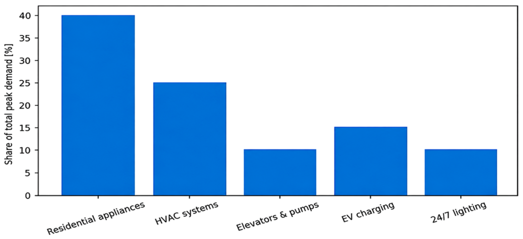
Figure 1 illustrates the main components of urban electricity consumption and their percentage contribution to the total peak demand.

Residential appliances—household electrical devices such as refrigerators, washing machines, kitchen equipment, and consumer electronics:

• HVAC systems—heating, ventilation, and air conditioning systems;
• Elevators and pumps—elevators and booster pumps used for water supply in multistorey buildings;
• EV charging—electric vehicle charging infrastructure;
• 24/7 lighting—lighting systems operating continuously, including corridor lighting, outdoor lighting, and emergency lighting.

The second largest component is represented by HVAC systems, which account for about 25% of the total load. EV charging infrastructure has emerged as a new load segment. Continuous lighting systems account for about 10% of the total load.

The load composition in urban low-voltage distribution networks cannot be adequately represented using traditional normative coefficients alone. Additional components such as HVAC systems, elevators, pumping units, and EV charging infrastructure significantly increase the maximum demand [19].

In this study a comfort coefficient is introduced into the load model in order to more accurately represent the real dynamics of urban electricity consumption [20].

The structural composition of loads must be considered when determining TS placement and service radius. The growing share of EV charging may require additional capacity reserves in low-voltage distribution networks in the future [21].

2.1.2. Introduction of the Comfort Coefficient and Its Physical Meaning

A distinctive characteristic of electricity consumption in urban environments is that, in modern buildings, the share of continuously or semi-continuously operating technological loads is increasing alongside traditional household loads. Electric-based heating systems have been increasingly implemented in urban buildings. In newly constructed residential buildings in Tashkent, Uzbekistan, electricity supply is increasingly replacing gas-based energy consumption [20].

Several additional urban load components, including HVAC systems, elevators, booster pumps, continuous lighting systems, and EV charging infrastructure, significantly increase the real electricity demand in modern buildings [22].

Traditional normative planning approaches do not always accurately capture the influence of these factors. This study proposes the introduction of “comfort level” as a separate coefficient, referred to as the comfort coefficient (k_com).

Based on this concept, the conventional load estimation model is extended, and the modified expression can be formulated as Equation (2) as follows:

$$P_{\mathit{ext}}={\displaystyle \sum _{i=1}^n}{P}_{\mathit{inst}.i}·k_{\mathit{dem}.i}·k_{\mathit{coin}.i}·k_{\mathit{com}.i}$$

(2)

where k_com depends on the building type and its operational technologies, and it is calibrated separately for residential, commercial, and office facilities [23].

The physical interpretation of the comfort coefficient can be expressed as the ratio between the actual (real) maximum demand and the normative maximum demand:

$$k_{\mathit{com}.i.}={\displaystyle \frac{P_{\mathit{real},\mathit{max}.i.}}{P_{\mathit{norm},\mathit{max}.i.}}}$$

(3)

The proposed comfort coefficient depends on regional climatic conditions, urban infrastructure characteristics, HVAC penetration level, and consumer energy usage behavior. Therefore, the coefficient values may vary for different cities and regions.

This ratio can be interpreted as follows: it indicates how much larger the observed maximum demand in real operation, P_real.max.i., is compared to the maximum demand estimated using the normative model, P_norm.max.i.. The comfort coefficient k_com essentially represents a deviation indicator from the normative estimation. If k_com.i. = 1.2, it means that the actual maximum load is 20% higher than the value predicted by the normative or specific load estimation method.

2.1.3. Determination of Comfort Coefficient Values Based on Building Types Using Data-Driven Analysis

The main principle in determining the comfort coefficient is that the more technologically equipped a building is, the higher the share of comfort-related electrical loads becomes. The value of the comfort coefficient (k_com) is directly related to the structural and operational characteristics of the building. The comfort coefficient (k_com) was not determined through subjective estimation or normative assumptions. For the analysis, 4000 representative load profiles were used.

These data were obtained from the Automated Electricity Metering and Monitoring System (AEMMS) database of the Joint Stock Company “Regional Electrical Networks” (“Hududiy elektr tarmoqlari” AJ) for consumer No. 784 in the Mirabad District of Tashkent, Uzbekistan [4].

For each object, the following parameters were available: maximum active power, average daily power, load factor, and building type (classification). To evaluate the load shape, each profile was normalized with respect to its maximum value: p_i(t) = P_i(t)/max_tP_i(t). This normalization approach enables consumers with different power levels to be compared within a unified load-shape framework [24].

The optimal number of clusters was determined using the Silhouette coefficient:

$$\mathit{Sil}\mathrm{h}\left(K\right) = {\displaystyle \frac{b-a}{\max (a,b)}}$$

(4)

where a—the average intra-cluster distance, while b—the average distance to the nearest neighboring cluster. The following main load typologies were identified: low-comfort residential buildings (private houses), medium-comfort 5–9 storey buildings, high-comfort 10+ storey buildings, commercial facilities, office buildings, and 24/7 operating facilities.

To account for extreme peak loads, the comfort coefficient is determined on the basis of the 95th percentile:

$$k_{\mathit{com}.c}={\displaystyle \frac{Q_{0.95}{(P}_{\mathit{max},\mathit{real}.c})}{P_{\mathit{norm},\mathit{max}.c}}}$$

(5)

where Q_0.95—the 95th percentile of the actual maximum load; c—building type index. By contrast, the 95th percentile offers a more appropriate compromise between design reliability and economic efficiency. For each building category, the 95% confidence interval was estimated by applying the bootstrap resampling method with 1000 iterations:

$${\mathit{CI}}_{95\%} = {\mu }_{k_{\mathit{com}}}\pm 1.96·{\sigma }_{k_{\mathit{com}}}$$

(6)

This confirms the stability of the comfort coefficient with respect to random fluctuations. The following statistically estimated values were obtained [25]:

• Private houses (1.05): these buildings usually do not have fully centralized HVAC systems, elevators, or shared pumping systems. The comfort-related load contributes only a small additional share;
• Five–nine storey residential buildings (1.20): such buildings typically include elevators, shared lighting, entrance corridors, and in some cases pumping systems. The deviation from the normative estimate becomes more pronounced;
• Ten+ storey residential buildings (1.40): higher comfort-related demand due to elevators, pumping systems, and HVAC technologies;
• Shopping centers (1.30): due to refrigeration equipment, ventilation, general lighting, and long operating hours, the load remains high and often close to peak levels;
• Office buildings (1.25): the presence of server rooms, general lighting, air-conditioning systems, and intensive daytime operation leads to elevated load levels during working hours.

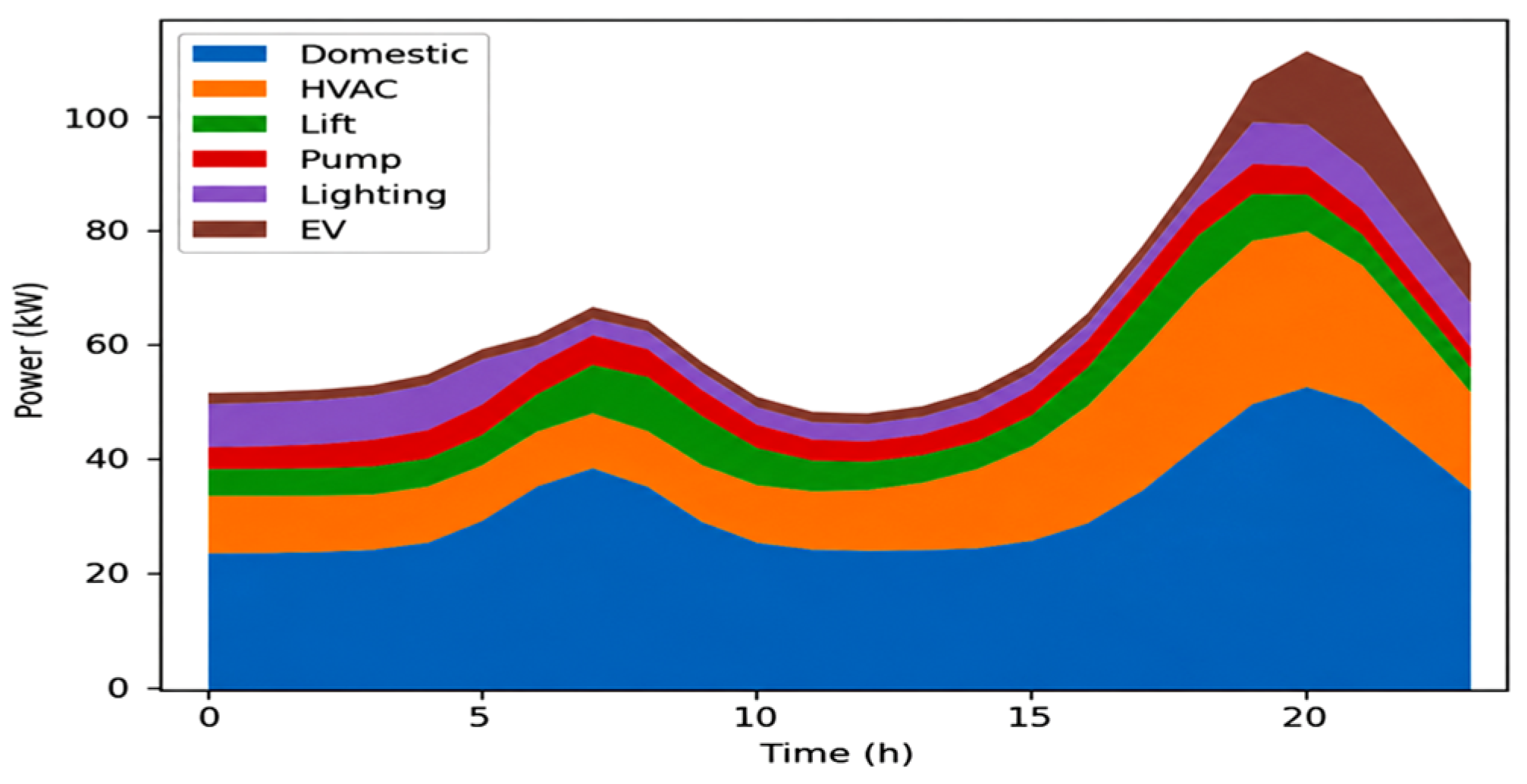
These values were integrated into the urban load model and subsequently incorporated into the optimization model for TS placement [26] (Figure 2).

The proposed coefficient values were calibrated using load-profile data from Tashkent city and may require regional recalibration when applied to other urban environments.

The comfort coefficient should not be interpreted as a fixed universal parameter. In long-term urban planning applications, its value should be periodically recalibrated considering future changes in HVAC penetration, EV charging infrastructure growth, consumer behavior, and urban development scenarios.

Nevertheless, the developed methodology demonstrates that even the introduction of k_com itself improves the realism of load estimation and reduces design errors [27].

The load decomposition process can be adapted for other cities using local statistical consumption data and regional load characteristics [28].

2.1.4. Total Calculated Load and Design Peak

In urban areas, the total calculated load should not be determined merely as a deterministic sum, but rather by taking into account the time-varying and statistical characteristics of different consumer segments [28,29]. The total active load is given by:

$$\sum P_{\mathit{ext}}(t)={\displaystyle \sum _{i=1}^n}{P}_{\mathit{inst}.i}·k_{\mathit{dem}.i}·k_{\mathit{coin}.i}·k_{\mathit{com}.c\left(i\right)}·{\mathsf{\psi }}_{c\left(i\right)}(t)$$

(7)

where i represents the consumer segment, such as residential, commercial, or office buildings; k_com.c(i)(t)—the time-varying comfort coefficient evaluated using the 95th percentile; and ψ_c(i)(t)—the normalized load-shape function obtained from the corresponding cluster centraoid:

$$P_{\mathit{des}.}=Q_{0.95} \{\sum P_{\mathit{ext}}(t\left)\right\}$$

(8)

This approach accounts for extreme peak days, while avoiding the creation of an excessively conservative reserve based on the absolute maximum (100%). Power system elements, such as transformers and cables, are loaded by current:

$$\sum S_{\mathit{des}.}={\displaystyle \frac{P_{\mathit{des}.}}{\mathit{cos}\phi }}$$

(9)

The use of this relationship is essential for the proper sizing of transformers and cables from the standpoint of current loading rather than active power alone [4,28,30,31].

In the planning of urban power supply systems, the load density σ serves as a key parameter, characterizing the power demand referred to a unit area of the territory, typically per square kilometer or square meter:

$$\sigma ={\displaystyle \frac{P_{\mathit{des}.}}{A}}$$

(10)

In contrast, when σ is low, the number of substations may be reduced; however, the resulting increase in service radius can negatively influence voltage regulation and supply reliability. σ should be regarded as one of the key input parameters in the subsequent optimization framework [32]. Load distribution in urban areas is inherently non-uniform. Consequently, the use of a single averaged value of σ tends to force TS placement toward an averaged solution, which may aggravate voltage drop and reliability issues in the most critical zones [33].

$$\sigma (x,y)={\displaystyle \frac{P_{des.}(x,y)}{A(x,y)}}$$

(11)

In the practical formulation, the study area is partitioned into M grid cells or zones, and the corresponding load density σ_m—evaluated for each of them [4].

$${\omega }_m={\displaystyle \frac{{\sigma }_m}{{\max }_j{\sigma }_j}} \Rightarrow 0<{\omega }_m\le 1$$

(12)

The service distance criterion in TS placement, defined as the average distance between consumers and the TS, is reformulated in a weighted form:

$$J_{\mathit{dist}}={\displaystyle \sum _{m=1}^M}{\omega }_m·d\left(m, \mathit{TS}\right(m\left)\right)$$

(13)

where d(·) represents the distance from the centroid of a zone, or from the corresponding load center, to the assigned TS [34], while TS(m) denotes the TS associated with zone m.

2.1.5. Determination of Transformer Quantity

In this article, one of the baseline design options is adopted as S_nom = 400 kVA. Although transformer loading is fundamentally governed by apparent power, the design load in this study is expressed in terms of active power. The corresponding active power limit for the transformer is written as follows [35,36,37]:

$$P_{\mathit{TS}}^{\mathit{max}}=S_{\mathit{op}}·\mathit{cos}\phi$$

(14)

This means that if cosφ is low, the transformer can carry a smaller active power load, since reactive power increases the current. The number of transformers is calculated on the basis of the following expression:

$$N_{\mathit{TS}}=⌈{\displaystyle \frac{P_{\mathit{design}}}{P_{\mathit{TS}}^{\mathit{max}}}}⌉$$

(15)

The rounding operation is necessary because, in a real power supply system, the number of transformers must be represented by a whole number [11,21,31].

The summary data for transformer capacity selection are presented in

Table 1. Transformer sizing summary: S_nom, k_load, cosφ, N_TS.

Parameter	Symbol	Value	Unit	Description
Total active load	Ptot	3180	kW	Estimated peak demand of the study area
Power coefficient	cosφ	0.92	–	Average load power coefficient
Total apparent power	Stot	3456	kVA	Stot = Ptot/cosφ
Transformer nominal power	Snom	400	kVA	Selected transformer rating
Load coefficient	kload	0.75	–	Allowable loading coefficient
Effective transformer capacity	Seff	300	kVA	Seff = kload·Snom
Max active power per TS	PTP.max	276	kW	PTP.max = Seff · cosφ
Required number of TS	NTS	12	units	NTS = Ptot/PTS.max

.

The maximum calculated active load for the studied urban area was found to be 3.18 MW (Table 1). To maintain operational reliability, the transformer loading coefficient was adopted as k_load = 0.75. The effective operating capacity of a transformer rated at 400 kVA is 300 kVA.

2.1.6. Mathematical Foundations of the Service Radius

The transformer service radius, denoted by R, represents the maximum permissible geometric spread of 0.4 kV low-voltage feeders extending from the TS to the connected consumers. The service radius is defined by three independent constraints:

• Voltage drop constraint;
• Current loading constraint;
• Reliability constraint.

Voltage Drop

In its basic form, the voltage drop is expressed as follows [23]:

$$∆U = \sqrt{3}·I·(R_l·\mathit{cos}\phi +X_l·\mathit{sin}\phi )$$

(16)

In this case, R_l and X_l denote the resistance and reactance of the line, respectively, and both parameters increase proportionally with its length [14]:

$$R_l=r^{\prime }·L, X_l=x^{\prime }·L$$

(17)

Here, r′ and x′ denote the active and reactive resistance of the cable per kilometer (Ohm/km), and L represents the length of the line (km) [15].

Next, the current expression is introduced. In a three-phase network, the active power is given by:

$$P=\sqrt{3}·U·I·\mathit{cos}\phi$$

(18)

From this, the current magnitude is determined by:

$$I={\displaystyle \frac{P}{\sqrt{3}·U·\mathit{cos}\phi }}$$

(19)

By combining expressions (16)–(19), the voltage drop is determined by the following expression:

$$∆U={\displaystyle \frac{P}{U·\mathit{cos}\phi }}\left(r^{\prime }·L·\mathit{cos}\phi +x^{\prime }·L·\mathit{sin}\phi \right)={\displaystyle \frac{P·L}{U}}\left(r^{\prime }+x^{\prime }·\mathit{tg}\phi \right)$$

(20)

Its physical meaning can be interpreted as follows:

-

r′ increases losses and voltage drop through the active component;

-

x′·tgφ sharply increases the voltage drop as the reactive load grows (that is, when tgφ is large).

In urban power networks, a decrease in cosφ may reduce the service radius even over the estimate given by the “R-only” model. While Equation (20) can be used as a design estimate, the final decision should be verified by AC load-flow analysis [26].

As a normative condition, the following is adopted:

$${\displaystyle \frac{∆U}{U}}\le {\mathsf{ϵ}}_U {\mathsf{ϵ}}_U=0.05$$

(21)

From this, the analytical maximum length of the line is determined as follows:

$$L_U^{\mathit{max}}={\displaystyle \frac{{\mathsf{ϵ}}_U·U^2}{P·\left(r^{\prime }+x^{\prime }·\mathit{tg}\phi \right)}} R_U\approx L_U^{\mathit{max}}$$

(22)

The physical meaning here is clear: as P or L increases, ΔU also increases; as F (the cross-sectional area) increases, ΔU decreases. To enlarge the service radius, it is necessary either to increase the conductor cross-section or to segment the demand [32,37,38].

Current Loading (Thermal) Constraint

The current limitation arises from the thermal operating condition of the cable line.

-

the cable line overheats;

-

the insulation ages;

-

the probability of failure increases.

In this case, the main limiting condition: I ≤ I_allow.

Using the current expression, the following relationship is obtained:

$${\displaystyle \frac{P}{\sqrt{3}·U·cos\phi }}\le I_{allow} \Rightarrow P\le \sqrt{3}·U·cos\phi ·I_{allow}$$

(23)

This condition is critically important: even if the voltage constraint is satisfied, violation of the current constraint puts the thermal operating condition of the cable at risk. The service radius is limited not only by the voltage criterion, but also by the thermal capacity of the cable [18,39].

At the analytical stage, Equation (23), together with the feeder load distribution, provides the following bound: R_I = maxR: I_l(R) ≤ I_allow, ∀l, where, I_l(R) is the current in line l for a topology dependent on R.

Reliability Constraint

In reliability analysis, the length of the 0.4 kV line directly affects the probability of outages.

$${\lambda }_l={\lambda }_0·L_l$$

(24)

where λ₀—the number of failures per year per 1 km (normative/statistical value).

$$\mathit{SAIDI}\approx {\sum }_l{\lambda }_{l}r·{\omega }_l$$

(25)

where r—the average restoration time. ω_l—the share of consumers affected when line l is disconnected, which depends on the network topology.

If the maximum permissible SAIDI value is denoted by SAIDI_max, then the maximum service radius is determined as follows:

$$R_{\mathit{rel}}={\mathit{SAIDI}}_{\mathit{max}}/\lambda ·r$$

(26)

Since service quality requirements are high in urban areas, this constraint should not be treated as a secondary factor, but rather as a central parameter in planning [18,23,26,36].

2.1.7. Optimal Service Radius

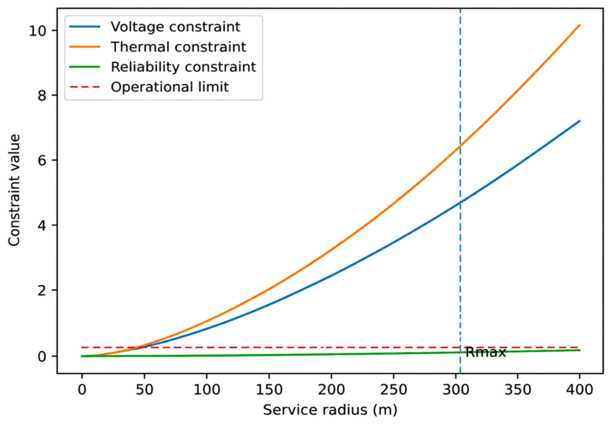
In practice, the service radius is limited by the most restrictive of the three conditions. Therefore:

$$R^{max}=min(R_U,{ R}_I,{ R}_{rel})$$

(27)

where R_U—the maximum radius determined by the voltage drop constraint; R_I—the maximum radius determined by the current loading constraint; and R_rel—the maximum radius determined by the reliability constraint.

As a result of optimization, the radius may be smaller than this value (to reduce losses), but if it exceeds this limit, at least one constraint will be violated [21,24,40].

In practical urban conditions, the actual installation location of a transformer substation may differ from the calculated optimal point due to land-allocation limitations, urban infrastructure constraints, or consumer-location characteristics. In such cases, if certain 0.4 kV feeder lengths exceed the recommended service radius, the modified configuration should be additionally verified through AC load-flow analysis. If voltage deviations, thermal loading limits, or reliability constraints are violated, additional technical measures such as feeder segmentation, larger cable cross-sections, or supplementary transformer substations should be considered.

The feasible region is subsequently used as the search space for the multi-objective optimization algorithm (Figure 3) [23,41,42].

2.1.8. Physical Interpretation and Design Implications

The physical meaning of the service radius is that it limits the supply capability of the transformer substation in three directions:

• Geometric effect: as the radius increases, the line length also increases (L↑);
• Electrical effect: as L increases, the resistance also increases (R_l↑);
• Energetic effect: as the resistance increases, the losses also increase, since: $P_{loss}=I^2·R_l$.

As a consequence of this:

-

ΔU ↑—the voltage quality deteriorates;

-

the thermal loading of the cable increases;

-

λ ↑ ⇒ SAIDI ↑—the quality of service deteriorates:

R_opt = f(P_loss, C_LCC, SAIDI)

(28)

The service radius is not merely a distance parameter, but a composite design variable that balances the threefold objective of energy efficiency (loss reduction), power quality (voltage level), and service performance (reliability). In urban power networks, selecting the radius empirically increases subjectivity, therefore, it should be defined using a mathematically grounded model such as Equation (27) [4,34,38,43].

2.2. Multi-Objective Optimization Model

2.2.1. Problem Formulation and Decision Variables

In urban 10/0.4 kV distribution networks, the problem of transformer substations (TS) placement must simultaneously satisfy the requirements of economic efficiency (CAPEX/OPEX), energy performance (loss minimization), voltage quality (compliance with EN/IEC limits), and quality of service (reliability indices such as SAIDI/SAIFI).

• Increasing the number of substations or adopting a denser placement strategy shortens feeder lengths and improves both losses and SAIDI, but increases CAPEX;
• Increasing the cable cross-section improves loss performance and voltage quality, but raises investment and installation costs;
• Increasing the service radius makes it possible to limit the number of substations, but worsens voltage drop, thermal current loading, and SAIDI.

The problem is formalized as a Constrained Multi-Objective Optimization Problem (CMOP), and the candidate solutions are evaluated through the Pareto-optimal set [36].

From this solution set (Figure 4), the NSGA-II algorithm is used to identify the Pareto-optimal alternatives that provide the most appropriate balance among technical, economic, and reliability objectives [14,18,29].

2.2.2. Decision Variables: Transformer Substations (TS) and the Service Radius R

The number of TSs is predetermined as a practical constraint: N_TS = 12.

Discrete Candidate Locations

The locations of TSs are selected from a discrete set of candidate points:

$$x_i\in \{1, 2, \dots , M\} i = 1, 2, \dots , n$$

(29)

where M—the number of candidate locations available for construction, GIS-based points filtered according to roads, zoning constraints, service accessibility, sanitary clearance distances, and related planning requirements [5,10,12,44].

Service Radius (R) as the Main Design Parameter of the Optimization Problem

In this study, the service radius R is introduced as a decision variable, since its influence is fundamental and is characterized by Equation (30). In particular, the radius:

-

defines the formation of transformer substation service zones (assignment);

-

directly determines feeder length and power losses;

-

has a strong impact on voltage constraints and on the reliability indices SAIDI/SAIFI.

$$R \in \left[R^{\mathit{min}}, R^{\mathit{max}}\right]$$

(30)

This interval is determined on the basis of Equation (27), derived in Section 2 from the physical bounds, namely the voltage constraint, thermal current limit, and reliability requirement [18,37].

Decision Vector

The optimization decision vector is formulated in the form given by Equation (31) below:

$$X = [x_1, x_2,\dots , x_{N_{\mathit{TS}}}, R]$$

(31)

The vector X represents a mixed-integer decision set composed of both discrete and continuous variables, which makes classical gradient-based methods practically inefficient and justifies the use of a heuristic multi-objective optimization algorithm [23,32,33]. The locations are selected, in accordance with practical planning conditions, from a discrete set of candidate points defined by Equation (32):

$$x_i\in \{1, 2, \dots , M\}$$

(32)

The discrete formulation restricts TS placement to points that are feasible for actual construction, thereby increasing the practical relevance and applicability of the optimization results [7,13,21,24]. The decision variables, their bounds, units, and constraints are presented in

Table 2. Decision variables and bounds: x_i (discrete), R (continuous), units, constraints.

Decision Variable	Type	Physical Meaning	Unit	Lower Bound	Upper Bound	Feasibility/Constraints (How Enforced)
xi, i = 1,…,NTS	Discrete (integer index)	i-TS (the candidate point index for the location of the transformer substation)	– (index)	1	M	xi ϵ {1,…, M}; uniqueness: xi ≠ xj) (i ≠ j); non-buildable zones are excluded; if duplicates occur, a penalty or repair mechanism is applied
R	Continuous (real)	the service radius of the TS (i.e., the maximum TS-to-consumer service distance in the 0.4 kV network), treated as a design parameter in the optimization	m	Rmin (200–250)	Rmax (350–400)	Main physical constraint: Rmax = min(RU, RI, Rrel)
aij (if the assignment is also optimized)	Discrete (binary)	assignment of consumer/zone j to transformer substation i (topology/clustering)	–	0	1	∑i aij = 1 (each j is assigned to only one TS.); distance constraint: dij ≤ R; consistent with the radial topology rule
Fl	Discrete (categorical)	Selection of the 0.4 kV cable cross-section	mm2	95	120	Fl ϵ {95,120}; thermal constraint Il ≤ Iallow (Fl); economic trade-off through CLCC
STS.i	Discrete (categorical)	Rated capacity of the TS transformer	kVA	250	400	Loading constraint: STS.i(X) ≤ kload·Snom; the number of TSs is constrained by capacity

.

This representation clarifies the mixed-integer nature of the formulated optimization problem and defines the feasible search domain for the solution algorithm [9,16,26,45].

2.2.3. Objective Functions: Three-Criterion Pareto Optimization

The optimization is carried out with respect to three principal criteria:

• LCC:

$$f_1\left(X\right)=C_{\mathit{LCC}}\left(X\right)$$

(33)

2.

Annual electrical energy loss:

$$f_2\left(X\right)=W_{\mathit{loss}}\left(X\right)[\mathrm{kWh}/\mathrm{year}]$$

(34)

3.

Reliability (SAIDI):

$$f_3\left(X\right)=\mathit{SAIDI}\left(X\right)[\mathrm{hours}/\mathrm{year}]$$

(35)

From these three expressions, the following multi-objective formulation is obtained:

$$\mathit{min}f\left(X\right)=[f_1\left(X\right), f_2\left(X\right),{ f}_3\left(X\right)]$$

(36)

where a single weighted-sum approach is not used as the primary solution mechanism; it may only be applied at a later stage to select one compromise solution.

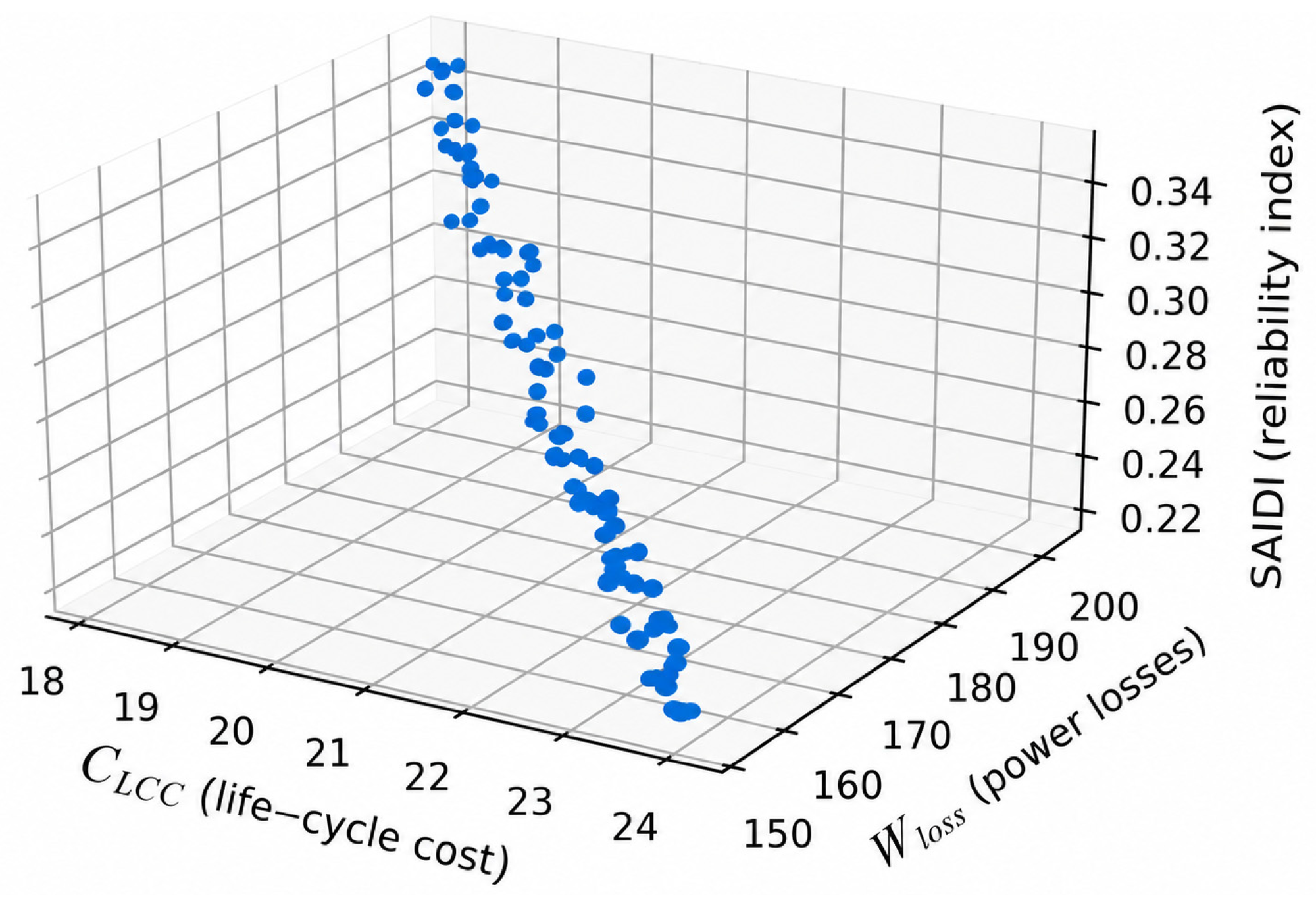
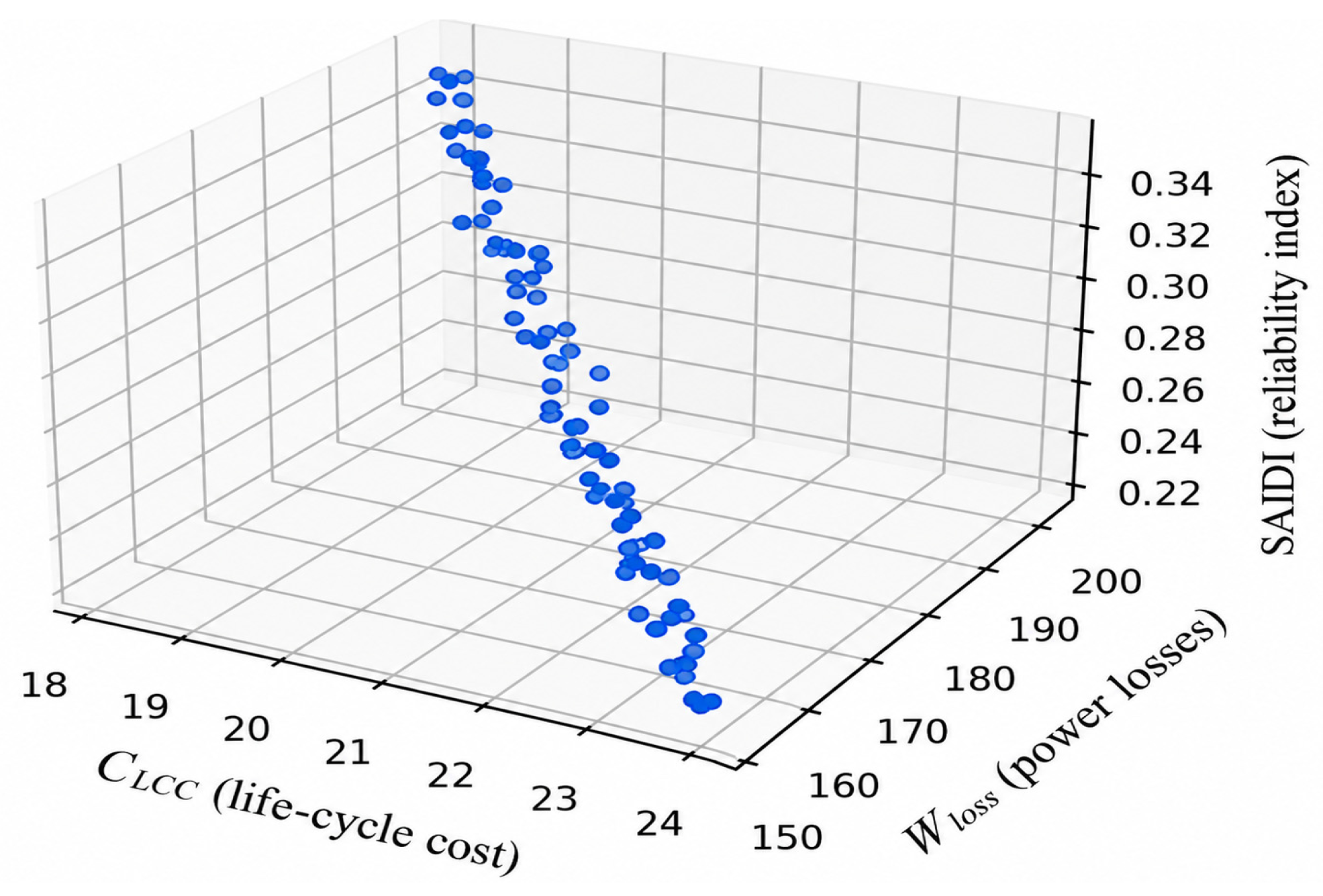
The presence of a Pareto front demonstrates that these three criteria cannot be simultaneously optimized to their best values: reducing cost is typically accompanied by increased losses or a deterioration in reliability performance (Figure 5).

The NSGA-II results provide a set of non-dominated alternatives, from which the decision-maker, that is, the network planner, selects the solution that best matches the preferred balance among technical, economic, and reliability priorities [18,39].

2.2.4. Why NSGA-II?

The selection of NSGA-II is justified by the following technical considerations. First, it identifies multiple solutions simultaneously on the basis of Pareto dominance. In urban power distribution planning, there is no single universal optimum; instead, a trade-off map is required. Second, it is well suited to nonlinear and black-box evaluations. Quantities such as W_loss, voltage profile, and transformer loading are obtained from PowerFactory load-flow simulations rather than from an explicit closed-form analytical function. Third, it is appropriate for mixed decision variables, where substation locations x_i are discrete, while the service radius R is continuous. Fourth, it can effectively handle technical constraints, including voltage limits, current-carrying capacity, and transformer loading, either through feasible-first ranking strategies or penalty-based integration. Fifth, the problem has a large combinatorial scale. With transformer substations and M candidate locations, the number of possible configurations grows on the order of (№12), making deterministic enumeration impractical [1,25,32,40,43,45].

Various algorithms may be applied to multi-objective optimization problems. However, in the planning of urban distribution networks, it is essential to identify a set of Pareto-optimal solutions because of the complex interactions among economic, technical, and reliability-related criteria. For this reason, the NSGA-II algorithm was selected in this study.

Table 3. Comparison of candidate optimization algorithms and justification for selecting NSGA-II.

Method	Optimization Principle	Strengths	Limitations	Suitability for This Research
Weighted-sum method	Multiple objectives are combined into a single objective using predefined weights	Simple implementation; low computational complexity	Requires predefined weights; cannot effectively capture non-convex Pareto fronts; solution sensitive to weight selection	Limited suitability because the planning problem involves conflicting objectives (CLCC, Wloss, SAIDI) and requires exploration of multiple trade-off solutions
Genetic Algorithm (GA)	Evolutionary algorithm based on selection, crossover, and mutation	Robust global search capability; widely used in power system optimization	Convergence may be slow; difficulty maintaining diversity of solutions in multi-objective problems	Applicable but less efficient for maintaining a well-distributed Pareto front in complex planning problems
Particle Swarm Optimization (PSO)	Population-based metaheuristic inspired by social behavior of particles	Fast convergence; simple parameter tuning; good performance for single-objective problems	May suffer from premature convergence; requires modification for multi-objective problems	Suitable for some power system problems, but less effective for generating diverse Pareto-optimal solutions
NSGA-II (Non-dominated Sorting Genetic Algorithm II)	Multi-objective evolutionary algorithm using non-dominated sorting and crowding distance mechanisms	Efficient Pareto front generation; good diversity preservation; widely validated in energy system planning	Higher computational cost compared with single-objective algorithms	Highly suitable for the present research because it can simultaneously optimize CLCC, energy losses, and reliability (SAIDI) while preserving solution diversity

presents a comparison of NSGA-II with other widely used optimization approaches [37].

For comparative consistency, the optimization algorithms considered in this study were evaluated under equivalent stopping criteria and comparable population-based parameter settings whenever applicable. In particular, the maximum number of iterations/generations and convergence evaluation principles were selected to ensure a fair comparison of optimization performance among the considered methods [39].

For fairness, all comparative optimization algorithms were executed under equivalent stopping conditions, including comparable population sizes, iteration numbers, and convergence evaluation principles.

Therefore, the NSGA-II algorithm was employed in this study to solve the multi-objective optimization problem. This algorithm makes it possible to identify the Pareto-optimal set of solutions, preserve solution diversity, and determine the most appropriate balance between technical and economic criteria [13].

2.2.5. Life-Cycle Cost Model: Discounted CAPEX + OPEX

General Definition

Energy infrastructure assets, such as TSs and 0.4 kV cable networks, typically operate over a service life of 20–30 years. Planning based solely on present-day capital expenditure may lead to distorted decisions.

$$C_{\mathit{LCC}}\left(X\right)=C_{\mathit{cap}}\left(X\right)+{\displaystyle \sum _{t=1}^T}{\displaystyle \frac{C_{\mathit{op}}(X,t)}{{(1+d)}^t}}$$

(37)

where C_cap—capital expenditure at year 0 (TS, cable, installation); C_op—operating expenditure in year t; T—base-case planning horizon (25 years); d—discount rate.

The discount rate determines the present value of one unit of future cost and reflects the following factors:

-

inflation and price escalation;

-

the cost of capital (interest rate, cost of borrowing);

-

investment risk and the opportunity cost of alternative uses of capital.

When d is low, energy losses and service-related expenses play a much stronger role. Performing a sensitivity analysis with respect to the discount rate d is methodologically justified [21,34,39].

Capital expenditures:

$$C_{\mathit{cap}}\left(X\right)=C_{\mathit{TS}}\left(X\right)+C_{\mathit{cable}}\left(X\right)+C_{\mathit{install}}\left(X\right)$$

(38)

where C_TS—the cost of transformers and substation equipment; C_cable—the cost of cables (depending on cross-sectional area and length); C_install—installation, excavation, design, and commissioning costs.

The Life Cycle Cost (LCC) model accounts for both capital and operating expenditures incurred throughout the entire service life of TSs and the distribution network infrastructure (

Table 4. Cost parameters and sources: cable unit cost, TS cost, installation multipliers.

Parameter	Description	Unit	Typical Value	Role in LCC Calculation
CTS	Transformer substation capital cost (400 kVA package substation)	USD/unit	28,000–35,000	Initial investment cost (CAPEX)
Ccable	0.4 kV distribution cable unit cost (95–120 mm2)	USD/m	18–25	Network construction cost (CAPEX)
kinst	Installation multiplier (civil works)	–	1.20–1.35	Adjusts total installation cost
Closs	Electricity price for loss evaluation	USD/kWh	0.07–0.10	Determines annual loss cost (OPEX)
Cmaint	Annual maintenance cost of TS	% of CAPEX	2–4%	Operation and maintenance cost (OPEX)
d	Discount rate	%	8–12%	Used for present value calculation
T	Project lifetime	years	25 (base case)	Base-case planning horizon used in LCC analysis

Note: In addition to the base-case value of 25 years, a sensitivity-analysis range of 20–30 years was also considered in the economic evaluation.

).

Operating Expenditures: The Cost of Energy Losses as the Main Component

The most significant component of operating expenditure is the cost associated with energy losses. It is determined using the following expressions:

$$C_{\mathit{op}}\left(X,t\right)=C_{\mathit{maint}}\left(X,t\right)+C_{\mathit{loss}}\left(X,t\right)$$

(39)

$$C_{\mathit{loss}}\left(X,t\right)=W_{\mathit{loss}}\left(X,t\right)·c_{\mathrm{e}}\left(t\right)$$

(40)

where c_e(t)—the price of 1 kWh of electrical energy.

The annual electrical energy loss is determined by the following expression [17]:

$$W_{\mathit{loss}}(X,t)=P_{\mathit{loss}}(X)·{\mathrm{h}}_{\mathit{eq}}$$

(41)

where ℎ_eq—equivalent operating hours (depending on the load profile). In practice, this parameter is selected on the basis of calculated load factors.

A sensitivity analysis with respect to the discount rate d is presented separately in a later section (Figure 6).

2.2.6. Electrical Energy Losses

Power losses in each line of the electrical network are determined according to the I²·R law:

$$P_{\mathit{loss}}(X) ={\displaystyle \sum _{l=1}^{N_L}}{I}_l^2(X) · R_l$$

(42)

where I_l—the current in line l, A; R_l—the active resistance of the line, Ohm.

The resistance of the electrical network line is determined by the following expression:

$$R_l = \rho ·{\displaystyle \frac{L_l}{F_l}}$$

(43)

It follows from the expression that losses can be reduced in two ways: by shortening the line length (L↓); and by increasing the cable cross-sectional area (F↑).

In general, the annual energy losses can be expressed in the following form:

$$W_{\mathit{loss}}(X, t) =\sum _{s=1}{P}_{\mathit{loss}}(X,s) · {\mathrm{h}}_s$$

(44)

where s—denotes the load scenario (morning/daytime/evening/night, or seasonal), h_s—the duration of scenario.

On this basis (

Table 5. Load scenarios: season/day-type, probability, hours.

Scenario s	Season	Day Type	Load Level Description	Probability ps	Duration hs (h/Year)
1	Winter	Weekday	Morning peak load	0.12	1050
2	Winter	Weekday	Daytime medium load	0.15	1300
3	Winter	Night	Low load	0.08	700
4	Summer	Weekday	Daytime HVAC peak load	0.18	1575
5	Summer	Evening	Residential peak load	0.14	1225
6	Summer	Night	Low load	0.10	875
7	Spring/Autumn	Weekday	Medium load	0.13	1135
8	Weekend	All seasons	Reduced commercial load	0.10	880

), the total annual energy losses are calculated using Equation (44) [5,30,46].

2.2.7. Reliability Model

SAIDI—the average outage duration per consumer per year (hours/year).

SAIFI—the average interruption frequency per consumer per year (interruptions/year).

Since SAIDI is the reliability index that most directly reflects the quality of electricity supply to consumers in urban areas, it is adopted as the primary reliability objective and is therefore minimized.

Relationship Between Failure Rate and Line Length

In 0.4 kV distribution lines, the probability of interruption increases as the line length becomes greater.

$${{\lambda }_l=\lambda }_0·L_l$$

(45)

where λ₀—the number of failures per year per 1 km (normative/statistical value); L_l—the length of line.

SAIDI:

$$\mathit{SAIDI}(X)={\displaystyle \frac{{\displaystyle {\sum }_{k=1}^{N_{\mathit{out}}}}{U}_k(X)·N_k(X)}{N_{\mathit{tot}}}}$$

(46)

where U_k—the duration of interruption k; N_k—the number of consumers affected by that interruption; N_tot—the total number of consumers. As a simplified approximation, the relationship SAIDI ≈ λ·r is sometimes used.

SAIFI—the number of interruptions per consumer per year is determined by the following relationship:

$$\mathit{SAIFI}={\displaystyle \frac{{\displaystyle {\sum }_{k=1}^{N_{\mathit{out}}}}{N}_k\left(X\right)}{N_{\mathit{tot}}}}$$

(47)

SAIDI is selected as the principal optimization criterion, since outage duration more directly reflects the quality of service experienced by consumers, where SAIFI is evaluated as an additional control indicator.

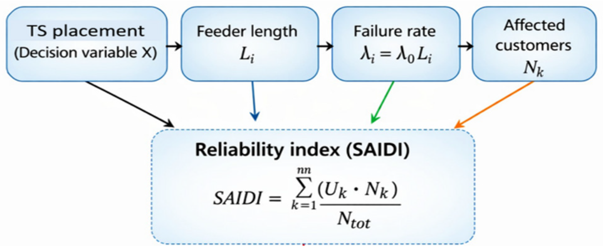
Figure 7 conceptually illustrates how the placement of transformer substations (TS) affects reliability indices in urban distribution networks. These factors directly influence the main reliability indicator of power supply, the System Average Interruption Duration Index (SAIDI) [47]. This conceptual model demonstrates that, in the optimization of urban distribution networks, the placement of TSs significantly affects not only energy losses and economic costs but also the reliability of power supply [23].

2.2.8. Constraints

Optimization involves not only minimizing f(X), but also ensuring that physical constraints are not violated.

Voltage constraint:

$$0.95\le U_i\left(\mathrm{X}\right)\le 1.05 \forall i \in \mathrm{buses}$$

(48)

Current constraint:

$$I_l\left(\mathrm{X}\right)\le I_{\mathit{allow}} \forall l \in \mathrm{lines}$$

(49)

Transformer loading constraint:

$$S_{\mathit{TS}.i}\left(\mathrm{x}\right)\le S_{\mathit{op}} i=1,\dots .,n$$

(50)

Radius (service assignment) constraint. Each consumer zone/node is connected to the nearest (or assigned) transformer substation, but the distance must not exceed R:

$$d\left(m, \mathit{TS}\left(m\right)\right)\le R, \forall m=1, \dots , M_z$$

(51)

where TS(m)—index of the transformer substation assigned to zone m.

2.2.9. Constraint Integration into NSGA-II

In the NSGA-II optimization procedure, technical constraints are handled using the constraint-dominance principle. Feasible solutions are prioritized over infeasible solutions, while infeasible solutions are ranked according to their aggregated constraint violation. The detailed formulation of the constraint violation measure and its implementation are presented in Section 2.3.6.

The total constraint violation for an infeasible solution is calculated as follows:

$$CV\left(X\right)=\sum _j\max (0,g_j(X\left)\right)$$

(52)

where $g_j\left(X\right)$—the magnitude of violation of constraint j (when U < 0.95 p.u., the deviation from the permissible limit is taken as the violation value).

If it is necessary to explicitly include a penalty function for the obtained model, it is written as:

$$f_p\left(X\right)=f\left(X\right)+\alpha CV\left(X\right)$$

(53)

2.2.10. NSGA-II Operators

Encoding. X_i: discrete indices (candidate locations)—integer encoding; R: continuous variable—real encoding. Discrete part: set-based crossover and swap mutation (exchanging TS locations or relocating one TS to another candidate point); Continuous part: SBX (simulated binary crossover) and polynomial mutation [5,12,21,40]. The main NSGA-II parameter values used in this study are presented in

Table 6. NSGA-II hyperparameters: population size, generations, crossover prob, mutation prob.

Parameter	Symbol	Value	Description	Rationale
Population size	Npop	120	Number of candidate solutions in each generation	Provides sufficient diversity of solutions for exploring the search space
Number of generations	G	120	Total number of evolutionary iterations	Ensures convergence of the Pareto front
Crossover probability	pc	0.9	Probability of recombination between two parent solutions	Encourages exploration of new solution regions
Mutation probability	pm	0.1	Probability of random modification of a solution	Prevents premature convergence
Selection method	–	Binary tournament	Selection based on non-dominated sorting and crowding distance	Maintains diversity along the Pareto front
Crossover type	–	Simulated Binary Crossover (SBX)	Recombination operator used in NSGA-II	Suitable for continuous decision variables
Mutation type	–	Polynomial mutation	Mutation operator applied to offspring	Helps maintain solution diversity

.

The selected parameter values were defined on the basis of recommendations commonly reported in the evolutionary optimization literature, and they ensured stable convergence of the Pareto front.

2.2.11. Co-Simulation Evaluation Loop Coupled with DIgSILENT PowerFactory

The objective functions f(X) and the associated constraints are obtained through PowerFactory load-flow calculations:

• The configuration X, consisting of the locations of 12 TSs and the service radius R, is specified;
• Consumers are assigned to substations according to the zonal assignment rule given in Equation (51);
• The feeder topology and corresponding line lengths are generated;
• The AC load-flow calculation is executed in PowerFactory, yielding U_i, I_l, and S_TS;
• P_loss is calculated and then converted into W_loss using Equation (44);
• Within the reliability module, SAIDI and SAIFI are determined using Equations (45)–(47);
• The LCC C_LCC is evaluated using Equations (37)–(40);
• The constraints in Equations (46)–(51) are checked, and the total constraint violation CV(X) is computed;
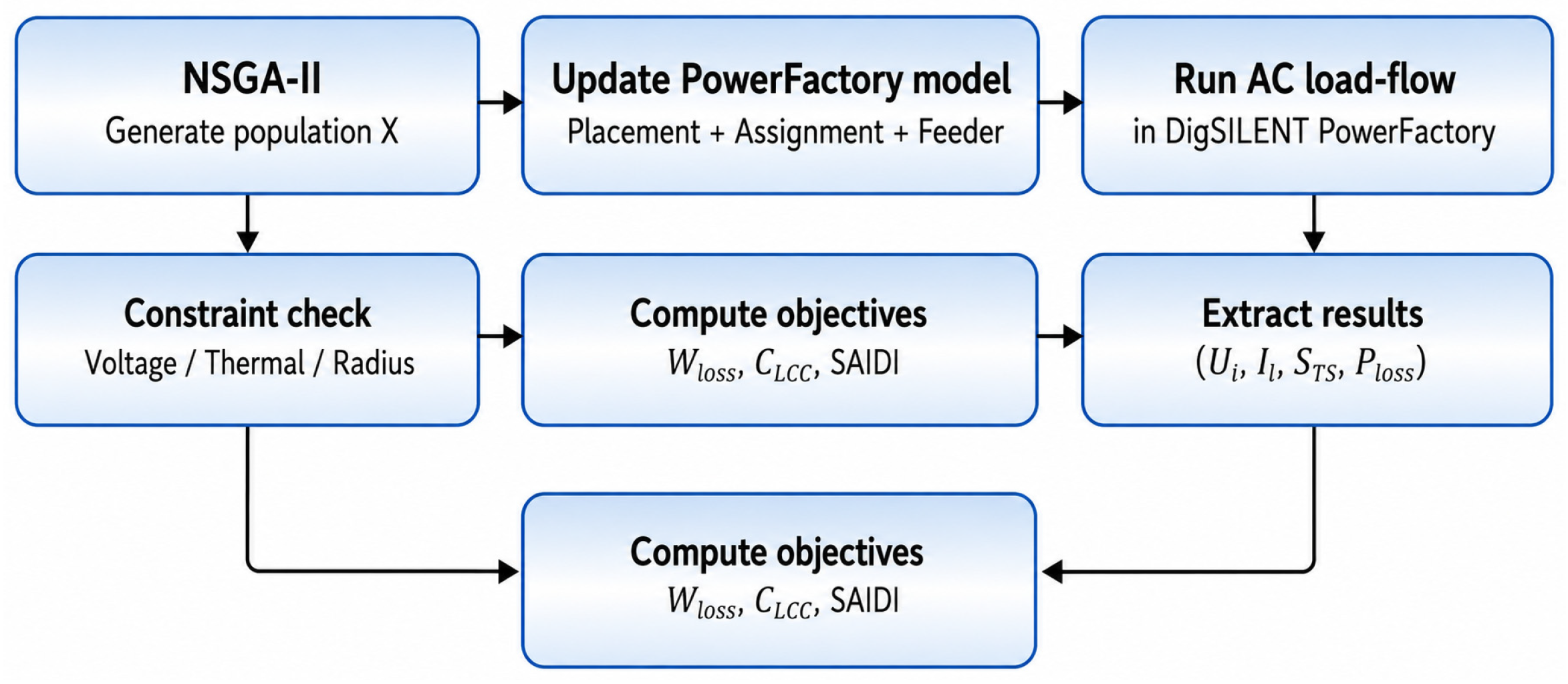
• The next population is updated through NSGA-II ranking and crowding-distance mechanisms.

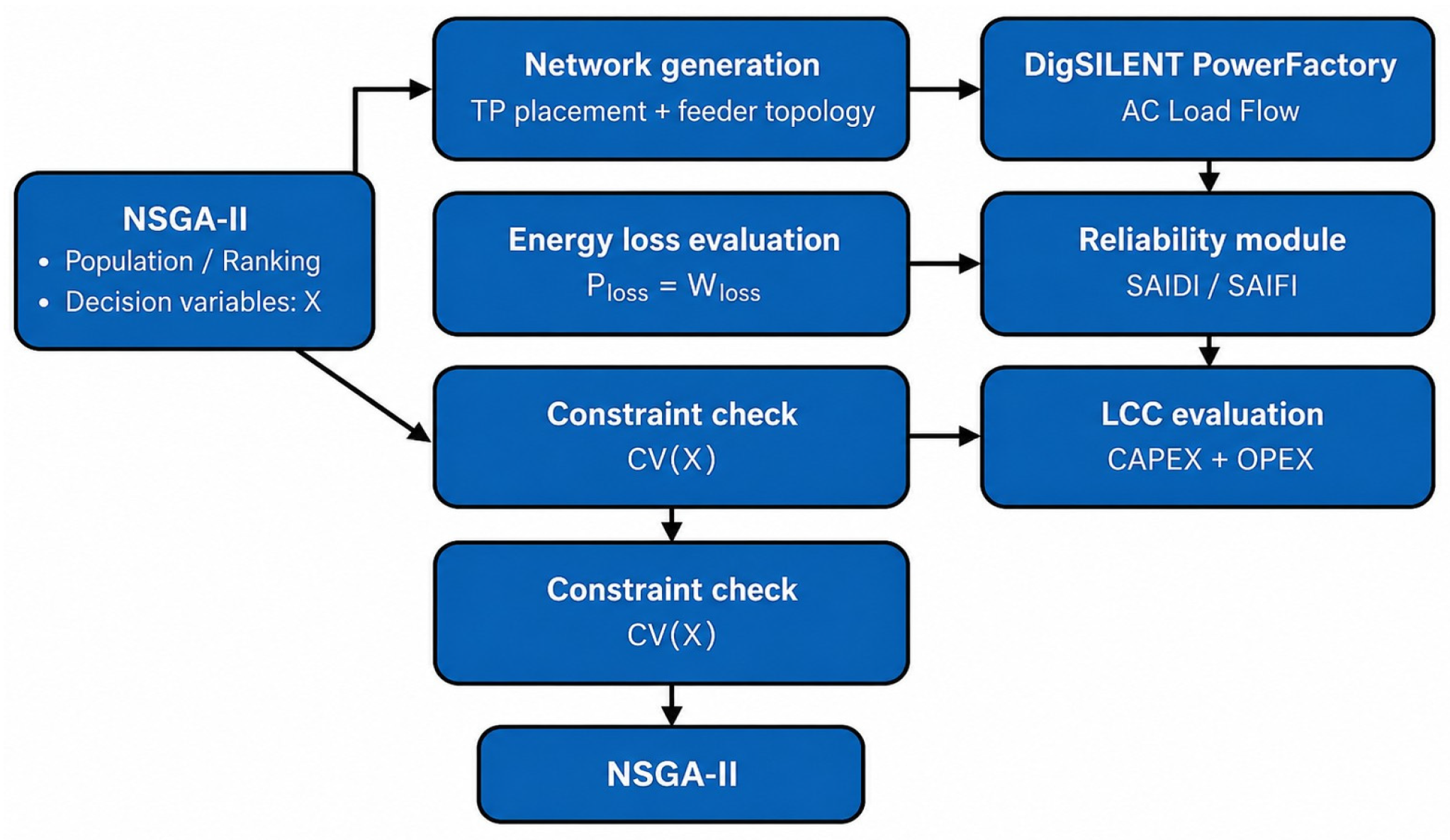
Figure 8 illustrates the co-simulation evaluation loop used in the proposed optimization framework. The NSGA-II algorithm generates candidate solutions X, which are used to create the network topology (TP placement and feeder configuration). The topology is then evaluated through DIgSILENT PowerFactory AC load-flow analysis to obtain electrical parameters. Based on these results, energy losses (W_loss), reliability indices (SAIDI/SAIFI), and life-cycle cost (CAPEX + OPEX) are calculated. Finally, the constraint violations CV(X) are checked and the results are returned to the NSGA-II population ranking process [7,35,48].

2.2.12. Mathematical Formulation

$$\min [C_{LCC}\left(X\right), W_{loss}\left(X\right),SAIDI(X\left)\right]$$

(54)

With constraints:

$$\left\{\begin{array}{c}0.95\le U_i\left(X\right)\le 1.05, \forall i\\ I_l\left(X\right)\le I_{\mathit{allow},l}, \forall l\\ S_{\mathit{TS},i}\left(X\right)\le S_{\mathit{is}\mathrm{h}}, i=1,\dots ,12\\ d\left(m, \mathit{TS}\left(m\right)\right)\le R, \forall m\\ x_i \in \left\{1,\dots ,M\right\}, i=1,\dots ,12\\ R^{\mathit{min}}\le R\le R^{\mathit{max}}\end{array}\right.$$

(55)

2.2.13. Selection of a Single Design from the Pareto Results

The NSGA-II algorithm provides a Pareto front consisting of multiple non-dominated solutions. However, for practical implementation, the developed model identifies one recommended design. This selection is performed using two approaches: the knee-point method, which entails identifying the point of maximum compromise on the Pareto curve; and TOPSIS, which functions by selecting the solution according to predefined priority scenarios [9,18,26,37].

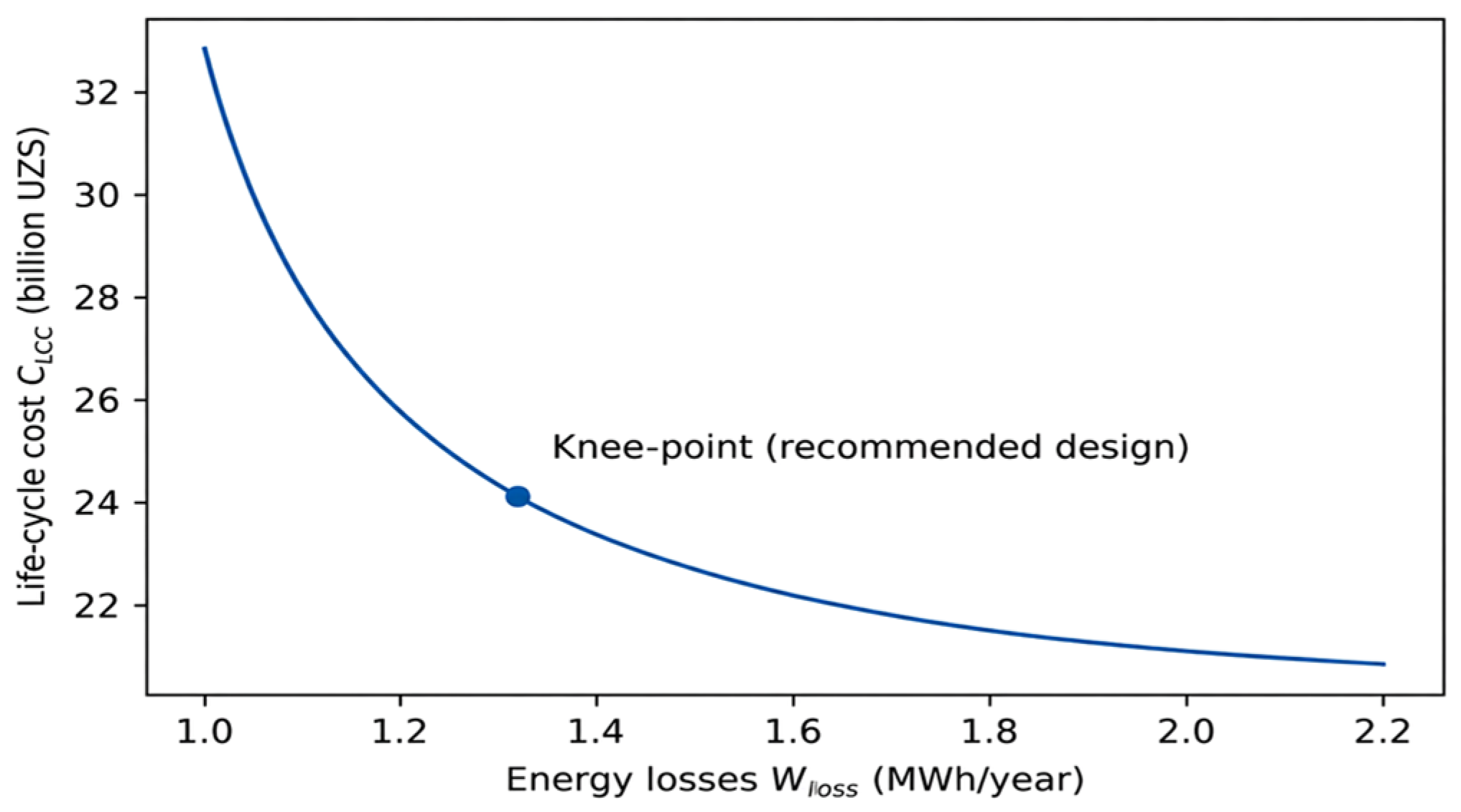
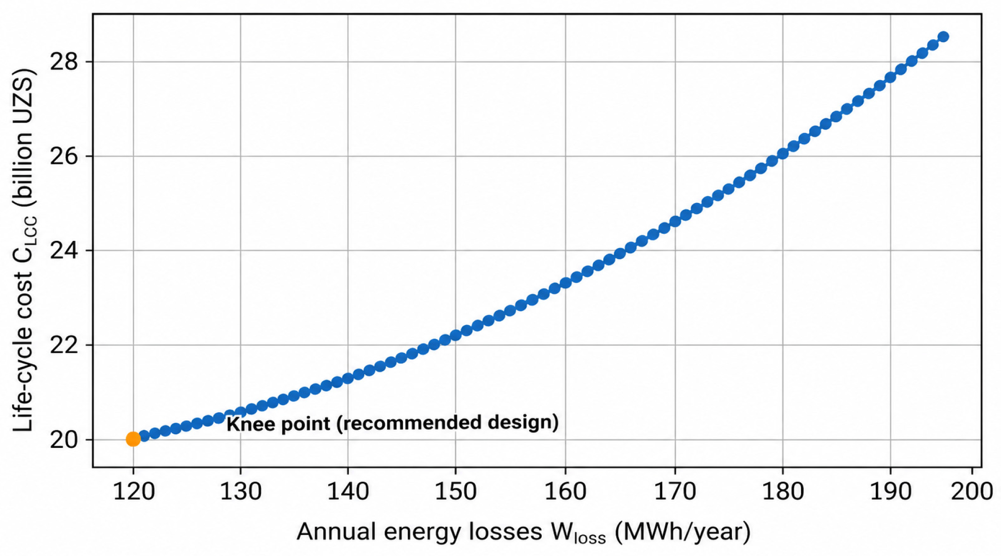
The knee-point on the curve is selected as the most balanced solution, since at this point any further improvement in one objective function would cause a significant deterioration in the other criterion (Figure 9). The knee-point is adopted as the recommended design for urban distribution network planning [5,31].

In addition, all technical constraints related to voltage limits and current loading have been satisfied (

Table 7. Recommended solution vs. baseline: cost, loss, SAIDI, constraint margins.

Metric	Baseline Design	Recommended Design (Knee-Point)	Improvement
Number of TS	12	12	–
Service radius (m)	350	300	Optimal trade-off
Life-cycle cost CLCC (billion UZS)	22.4	20.8	−7.1%
Annual energy loss Wloss (MWh/year)	178	142	−20.2%
SAIDI (hours/year)	0.28	0.23	−17.9%
Voltage constraint margin	4.1%	3.2%	Within limit
Thermal loading margin	18%	22%	Improved

) [18,26].

2.3. NSGA-II Algorithm and Its Integration with DIgSILENT Power Factory

2.3.1. Theoretical Foundations for the Selection of the Metaheuristic Approach

The problem of placing 12 transformer substations (TS) in urban 10/0.4 kV distribution networks is characterized by the following features [9,14,33,41,47]:

• Multi-objective: C_LCC, W_loss, and SAIDI are minimized simultaneously;
• Strongly constrained: voltage limits, line thermal current limits, transformer loading limits, and service radius constraints must be satisfied;
• Combinatorial (discrete): TSs are selected from GIS-based candidate locations;
• Nonlinear and black-box evaluation: the objective functions depend on the AC load-flow solution;
• Mixed decision variables: x_i are discrete, while the service radius R is continuous.

The objective functions are determined based on the results of the DIgSILENT AC load-flow analysis:

$$f\left(X\right)=\left[C_{\mathit{LCC}}\left(X\right), W_{\mathit{loss}}\left(X\right), \mathit{SAIDI}\left(X\right)\right], X=[x_1,\dots ,x_{12},R]$$

(56)

During the NSGA-II optimization process, each candidate solution was evaluated in the DIgSILENT PowerFactory environment using AC load-flow analysis. The simulation model was developed considering the technical, operational, and reliability parameters of the urban 10/0.4 kV distribution network. To ensure reproducibility, the main parameters and their values used in the DIgSILENT PowerFactory model are provided (

Table 8. Main DIgSILENT PowerFactory simulation parameters.

Parameter	Symbol	Value	Unit	Description
Distribution network voltage	Unom	10/0.4	kV	Nominal voltage level of the urban distribution network
Study area	A	0.48	km2	Investigated urban territory in Tashkent city
Total active load	Ptot	3180	kW	Calculated peak active load of the study area
Power factor	cosφ	0.92	–	Average load power factor
Transformer nominal capacity	Snom	400	kVA	Base-case transformer rating
Transformer capacity range	STS.i	250–400	kVA	Candidate transformer capacities used in optimization
Cable cross-sectional area	Fl	95–120	mm2	Candidate LV cable sizes
Voltage constraint	Ui	0.95–1.05	p.u.	Permissible voltage deviation limits
Service radius range	R	200–400	m	Optimization range for TS service radius
Load-flow calculation type	–	AC Load Flow	–	Power flow analysis mode in DIgSILENT
Optimization algorithm	–	NSGA-II	–	Multi-objective optimization method
Reliability index	–	SAIDI	h/year	Reliability performance criterion
Discount rate	d	8–12	%	Economic discount rate used in LCC analysis

).

The practical reasons for choosing NSGA-II are as follows [5,13,26]:

• It returns the Pareto front in a single run;
• It is suitable for mixed discrete–continuous decision variables;
• It operates robustly in nonlinear, constrained, and simulator-based evaluations;
• Being population-based, it is well suited for parallel evaluation, since each individual solution can be evaluated through a separate load-flow calculation [9].

Unlike conventional GA-based approaches, the proposed framework does not rely solely on parameter tuning or structural modification of the optimization algorithm. The scientific novelty of the proposed approach lies in the integrated multi-objective optimization environment, where NSGA-II is directly coupled with DIgSILENT PowerFactory AC load-flow simulations, GIS-based transformer substation candidate selection, life-cycle cost modeling, and SAIDI-oriented reliability assessment under real urban operational constraints. In contrast to many recent hybrid metaheuristic approaches, the proposed framework simultaneously considers mixed discrete–continuous decision variables, nonlinear simulator-based evaluations, technical network constraints, and urban service-radius limitations within a unified optimization structure [13].

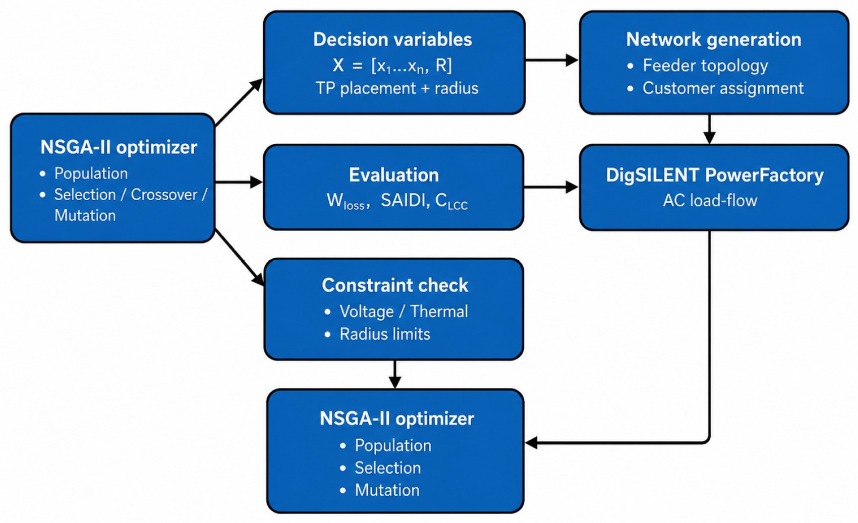
The decision vector is expressed as X = [x₁, x₂,…, x₁₂, R], where x_i represents discrete variables corresponding to the locations of TSs, and R denotes the continuous service radius parameter (Figure 10) [31,35,42].

The resulting network model is then transferred to the DIgSILENT PowerFactory environment, where AC load-flow calculations are performed. Node voltages, line current loadings, and transformer loadings are determined [2].

In addition, technical constraints such as voltage limits, line current limits, and the service radius constraint are verified.

2.3.2. Mathematical Model of NSGA-II: Dominance, Crowding Distance, and Generation Update

The NSGA-II algorithm operates on a population of solutions P_t, which represents the set of candidate solutions in the t-th generation [16,17,18,26,36]:

$$P^t = \{X_1^t,{ X}_2^t,\dots ,{ X}_N^t\}$$

(57)

For each X_i, the objective function value f(X_i) is obtained from the PowerFactory evaluation results.

Pareto Dominance

A solution X_a is said to dominate another solution X_b (X_a ≺ X_b) if the following conditions are satisfied:

$$\forall k: f_k\left(X_a\right)\le f_k\left(X_b\right) \mathrm{and} \exists k: f_k\left(X_a\right)\le f_k\left(X_b\right)$$

(58)

Crowding Distance (Maintaining Diversity)

To preserve the diversity of solutions within the Pareto front, the crowding distance is calculated.

$$\mathit{CD}\left(X_i\right)={\displaystyle \sum _{k=1}^K}{\displaystyle \frac{f_k\left(X_{i+1}\right)-f_k\left(X_{i-1}\right)}{f_k^{\mathit{max}}-f_k^{\mathit{min}}}}$$

(59)

NSGA-II preserves not only the best solutions but also those that are both Pareto-optimal and sufficiently diverse.

2.3.3. Mixed Encoding of Discrete Placement and Continuous Radius

The placement of TSs is represented using discrete indices:

$$x_i \in \{1,2,\dots ,M\} i = 1,\dots ,12$$

(60)

While the service radius is continuous:

$$R \in \left[R^{\mathit{min}}, R^{\mathit{max}}\right]$$

(61)

Operators for Discrete Genes (TS Indices)

For the discrete part, the standard real-coded operators of NSGA-II cannot be directly applied. Set-based operators are used [12,21,22,32,49]. Swap mutation: one or two randomly selected TS indices are replaced with other available candidate locations.

Operators for the Continuous Gene (R)

For the service radius, commonly used NSGA-II operators are applied: SBX (Simulated Binary Crossover) and Polynomial mutation [31,37,40]:

$$P^t = \{X_1^t,{ X}_2^t,\dots ,{ X}_N^t\}$$

(62)

Any values exceeding the admissible bounds were returned to the feasible interval by means of a clipping operator (

Table 9. Mixed operator’s summary: discrete crossover/mutation + continuous SBX/polynomial.

Operator Type	Variable Type	Operator Name	Description	Key Parameters
Crossover	Discrete genes xi	Set-based crossover	Two parent TP index sets are combined using union/intersection operations and then filtered to retain 12 unique candidate locations	set size = 12
Mutation	Discrete genes xi	Swap mutation	One or two transformer indices are replaced by randomly selected unused candidate nodes	mutation probability pm
Repair	Discrete genes xi	Local repair	If duplicate indices appear after crossover or mutation, they are replaced by the nearest available candidate node or randomly repaired	distance rule
Crossover	Continuous gene R	SBX (Simulated Binary Crossover)	Generates offspring service radius values by probabilistically combining parent solutions while preserving distribution properties	pc, distribution index ηc
Mutation	Continuous gene R	Polynomial mutation	Applies small perturbations to the radius value to maintain diversity in the population	pm, distribution index ηm
Boundary control	Continuous gene R	Clipping	Ensures that mutated radius values remain within the feasible interval [Rmin, Rmax]	bounds Rmin, Rmax

) [21,24,32,42].

2.3.4. Duplicate Prevention and Feasibility Repair

In practical implementation, it is not possible for 12 TSs to be placed at the same location. The following strict condition is imposed:

$$x_p\ne x_q, \forall p\ne q$$

(63)

If duplicates occur, a repair procedure is applied:

-

the duplicated TS index is identified;

-

the nearest available candidate location is determined;

-

the index is reassigned to that location.

If the repair cannot be performed (if there are insufficient candidate locations), the solution is marked as infeasible and receives a lower priority through the constraint-handling mechanism.

2.3.5. Selection and Scientific Justification of NSGA-II Parameters

Since the PowerFactory load-flow evaluation is computationally expensive, it is not practical to use a very large population size or a very high number of generations. The algorithm parameters are selected by balancing convergence quality against computational time [12,21,32]:

• Population size: N = 80~150 (practical value: 120);
• Number of generations: G = 80~200 (practical value: 120);
• Crossover probability: p_c = 0.8~0.95;
• Mutation probability: for discrete genes $p_m^{disc}$ ≈ 1/12, and for the radius $p_m^R$ ≈ 0.1.

The physical rationale for this choice is as follows: if the population size is too small, the Pareto front is poorly covered; if it is too large, the number of PowerFactory calls increases significantly, which may cause the computation to stall or become impractically slow [22].

Additional sensitivity tests demonstrated that the selected NSGA-II parameter configuration provided stable convergence behavior and consistent Pareto-front generation under repeated optimization runs [32].

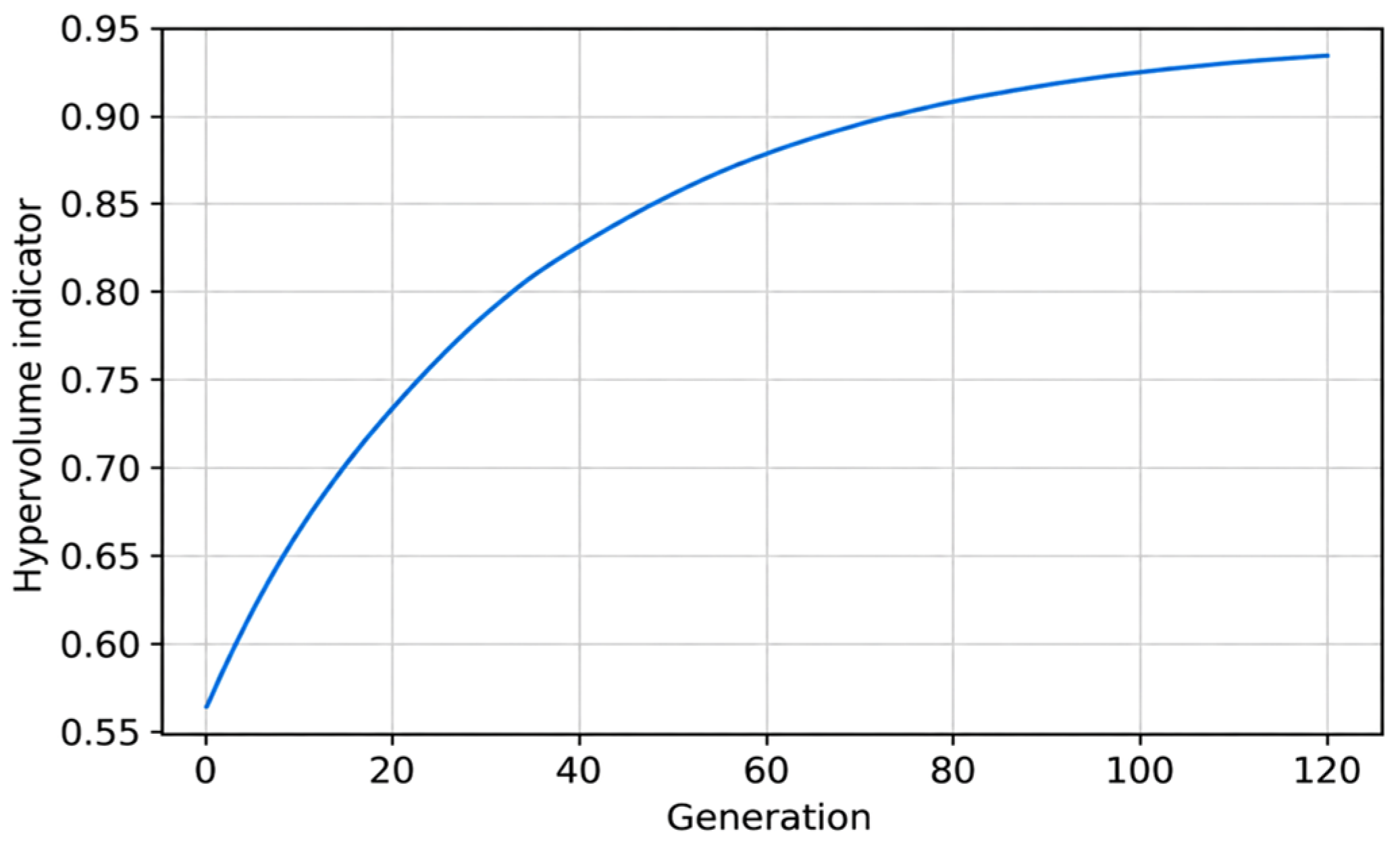
Figure 11 illustrates the convergence process of the NSGA-II optimization algorithm using the hypervolume indicator. This trend confirms that the selected NSGA-II parameters (population size and number of generations) are sufficient for the given optimization problem.

2.3.6. Behavior Under Constraint Violations

Constraint verification is performed using the results obtained from the PowerFactory simulations:

• Voltage: 0.95 ≤ U_i ≤ 1.05;
• Current: I_l ≤ I_allow,l;
• Transformer: S_TS,I ≤ S_op;
• Radius: d(m,TS(m)) ≤ R.

For constraint handling in NSGA-II, the feasible-first rule is applied:

-

A feasible solution always dominates an infeasible one;

-

If both solutions are infeasible, the solution with the smaller constraint violation is preferred;

-

If both solutions are feasible, Pareto dominance is applied.

The aggregated measure of constraint violation is defined using the following model [12,22,32,37]:

$$\begin{gathered} CV\left(X\right)={\sum }_i\max \left(0, 0.95-U_i\right)+{\sum }_i\max \left(0, U_i-1.05\right)+{\sum }_l\max \left(0, I_l-I_{allow,l}\right)+{\sum }_i\max \left(0, S_{TS.i}-S_{is}\right)+ \\ +{\sum }_m\max \left(0, {d\left(m,TS\left(m\right)\right)-R}_i\right) \end{gathered}$$

(64)

This formulation does not require an explicit penalty term; NSGA-II uses the constraint violation measure CV directly within its dominance ranking procedure. In the implementation stage, all constraint violation terms were internally scaled relative to their allowable limits before aggregation within the NSGA-II ranking procedure. To avoid disproportionate influence of constraints with larger numerical magnitudes, all constraint violation components were evaluated in normalized relative form with respect to their allowable limits. This normalization transforms the violation terms into dimensionless quantities and improves the stability of NSGA-II ranking during constrained optimization.

$$f_k^{pen}\left(X\right)=f_k\left(X\right)+\alpha CV\left(X\right)$$

(65)

2.3.7. NSGA-II–DIgSILENT Integration

The integration operates as follows [24,28,39].

Model Update. For each solution X:

• The TS objects in the PowerFactory model are placed according to the 12 selected candidate indices;
• In accordance with the service radius R, zones/consumers are assigned to substations using a nearest-feasible assignment rule;
• The 0.4 kV radial feeders are reconstructed, and the lengths/connections of the corresponding feeders are updated.

AC Load-Flow and Extraction of Performance Indicators

The PowerFactory load-flow analysis is then executed, from which the following quantities are obtained:

• U_i: bus voltages;
• I_l: line currents;
• S_TS,i: transformer loading;
• P_loss: active power losses.

Subsequently, on the basis of the formulations developed in Section 3, the following indicators are evaluated:

• W_loss (scenario/hour-based);
• C_LCC (discounted);
• SAIDI/SAIFI (based on topology and the affected service area).

Each individual solution is represented by the vector X = [x₁, x₂,…,x₁₂, R], where xi denotes the discrete location indices of TSs and R represents the continuous service radius parameter (Figure 12) [1,12,21,24,32].

For each generated solution, the following operations are performed in the DIgSILENT PowerFactory model:

• TSs are placed at the selected GIS candidate locations;
• Consumers are assigned to the corresponding substations based on the service radius;
• The topology of the 0.4 kV radial feeders is created or updated.

After that, AC load-flow calculations are executed in the PowerFactory environment, and the following technical parameters are obtained:

• Bus voltages (U_i);
• Line current loadings (I_l);
• Transformer loading (S_TS);
• Active power losses (P_loss).

Based on these results, the optimization objectives are evaluated:

• Electrical energy losses (W_loss);
• Life-cycle cost (C_LCC);
• Power supply reliability (SAIDI).

In addition, constraints related to voltage limits, line thermal limits, and service radius are verified.

Within the proposed co-simulation framework, NSGA-II generated candidate transformer substation placement solutions and transferred the corresponding decision variables to the DIgSILENT PowerFactory environment. For each candidate solution, AC load-flow analysis was performed to calculate node voltages, line loadings, transformer loading levels, power losses, and reliability-related operational parameters. The obtained simulation results were then returned to the NSGA-II optimization environment, where objective functions and constraint violations were evaluated during the Pareto-ranking process [12].

2.3.8. NSGA-II–PowerFactory Integration Algorithm

The optimization process was terminated when the maximum number of generations was reached or when no significant improvement in the Pareto front was observed during consecutive generations. The integrated NSGA-II–AC optimization framework is presented in Algorithm 1.

Algorithm 1. Integrated NSGA-II–AC Optimization Framework

Initialize population size N, generations G; Generate initial feasible individuals X = [x1…x12, R]; For each individual:     3.1 Update PowerFactory topology and assignments;     3.2 Run AC load-flow;     3.3 Extract Ui, Il, STS, Ploss;     3.4 Compute Wloss, CLCC, SAIDI, and CV(X). 4. Non-dominated sorting + crowding distance; 5. For generation t = 1…G:     5.1 Parent selection (binary tournament using rank + crowding);     5.2 Apply mixed crossover (set-crossover + SBX for R);     5.3 Apply mixed mutation (swap mutation + polynomial mutation for R);     5.4 Repair duplicates and bound R;     5.5 Evaluate offspring via PowerFactory loop (step 3);     5.6 Merge parent + offspring, re-sort, keep best N; 6. Return Pareto set P∗ and recommended knee-point solution.

The workflow illustrates the generation of feasible mixed-encoded solutions, PowerFactory-based AC load-flow evaluation, calculation of W_loss, C_LCC, SAIDI, and CV(X), followed by non-dominated sorting, crowding-distance preservation, offspring generation, and iterative Pareto-front refinement until the final Pareto set and recommended Knee-point solution are obtained (Figure 13) [12,32,36,37,42,48].

Each point corresponds to an alternative network configuration defined by the placement of TSs and the associated service radius parameter [21,25].

The knee-point represents the region of maximum curvature on the Pareto curve and provides the most balanced compromise between the conflicting objectives [32,42,48].

This point was selected as the recommended design, since it ensures the most appropriate balance between reducing energy losses and minimizing the LCC.

2.3.9. Python–DIgSILENT Integration

The integration is organized through a Python 3.10-based control layer [1,3,14,31]:

• Python: NSGA-II search engine (population management, genetic operators, ranking);
• PowerFactory API: model updating and execution of load-flow calculations;
• Reliability/LCC module: evaluated in Python or in a separate external module;
• Outputs: Pareto set, convergence diagnostics, and export-ready data for figures and table.

Architecture:

• NSGA-II—search and Pareto optimization;
• DIgSILENT PowerFactory 2021 —physical AC load-flow verification;
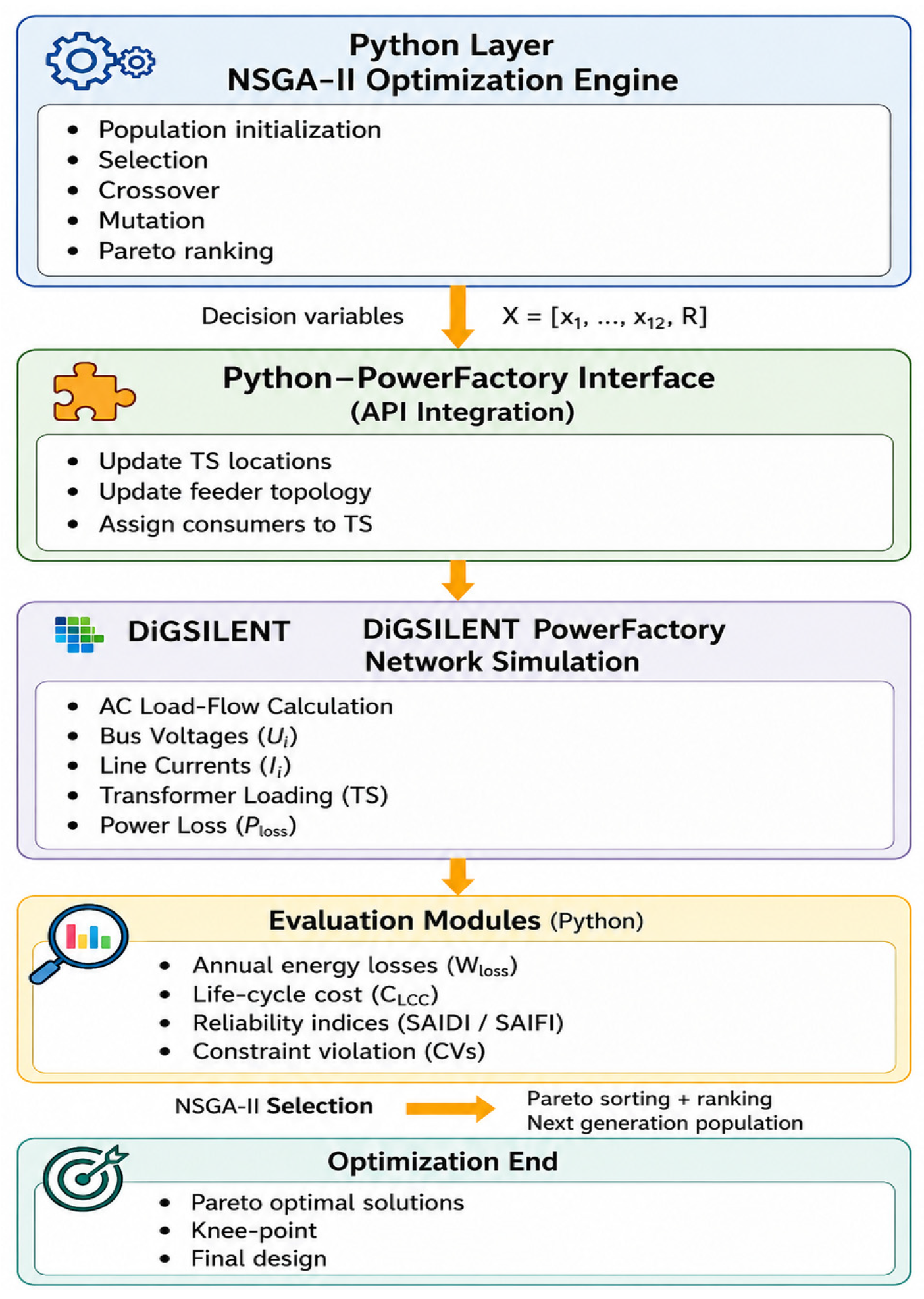
• Python—integration, automation, logging, and reproducibility (Figure 14).

Next, through the Python–PowerFactory API interface, the TS locations are updated, feeder topology is generated, and consumers are assigned to the corresponding substations [5,29,35,40,50].

These results are then transferred back to the Python evaluation modules, where the optimization objectives-annual energy losses (W_loss), LCC (C_LCC), and reliability indices SAIDI/SAIFI-as well as constraint violations are computed [42,48].

Finally, the recommended network configuration is selected using the knee-point method, which provides the most balanced compromise among the optimization objectives [8,12,14].

Table 10. Reproducibility settings: random seed, PF version, solver settings, tolerance, scenario set.

Category	Setting	Recommended Value/Description	Purpose (Reproducibility Impact)
Randomness control	Random seed	seed = 2025 (fixed)	Reproducing the results of NSGA-II selection, mutation, and repair
Algorithm run protocol	Independent runs	10 runs (using the same predefined list of seeds)	Statistical verification of Pareto front stability
PowerFactory version	PF release	DIgSILENT PowerFactory 2021	Version differences may affect solver results
PowerFactory project snapshot	Project file	Snapshot	Ensuring that the model topology and parameters remain identical
Load-flow solver type	AC solver	Newton–Raphson (AC load-flow)	Obtaining the nonlinear solution with the same solver
Solver initialization	Initial conditions	Flat start (or last converged)—one fixed protocol	Reducing differences in convergence behavior and local solutions
Convergence tolerance	Voltage mismatch tol.	10−6 p.u. (PF default + strict setting)	Numerical stability and repeatable results
Max iterations	Iteration cap	30–50 (fixed)	Preventing inconsistent solver stopping behavior across different runs
Constraint evaluation	Voltage limits	0.95 ≤ Ui ≤ 1.05 p.u.	Ensuring consistent feasible/infeasible classification
Constraint evaluation	Thermal limits	Il ≤ Iallow (according to the cable cross-section)	Standardized verification of thermal constraints
Constraint evaluation	Transformer loading	STS.i ≤ Sop	Ensuring that transformer loading constraints are evaluated under the same criterion
Scenario set (loss energy)	Load scenarios	s = 1…S: season/day-type	Computing Wloss using the same scenario set
Scenario probabilities	Probability model	ps fixed (calibrated)	Ensuring that scenario weights remain unchanged across different runs
Scenario hours	Hours per scenario	hs fixed (distribution over 8760 h)	Reproducibility of the annual loss calculation
Economic parameters	Discount rate	d = 0.10 (base case) + sensitivity analysis (0.06–0.14)	Comparison and sensitivity analysis of CLCC results
Cost database	Unit costs	Cable/TS/installation costs	Source and recalculation basis of economic results
Logging	Evaluation log	KPI values and constraint margins for each individual (CSV)	Supporting audit, debugging, and responses to reviewer questions
Output format	Export standard	Pareto set, knee-point, plots data (CSV/Excel)	Facilitating the redrawing of figures and tables

summarizes the main reproducibility settings adopted in the study, including randomness control, algorithm run protocol, PowerFactory solver configuration, constraint evaluation rules, scenario definitions, economic parameters, and output logging standards.

As practical strategies for reducing the computational burden, the following measures are incorporated into the methodology [9,12,32,33]:

• Warm start: if the next individual has a similar topology, the solver initial guess is retained;
• Feasibility pre-check: the service radius and duplicate placements are verified before sending the solution to PowerFactory, thereby reducing unnecessary load-flow calls;
• Parallel evaluation: since the individuals in the population are independent, they can be evaluated in parallel using a multi-process framework.

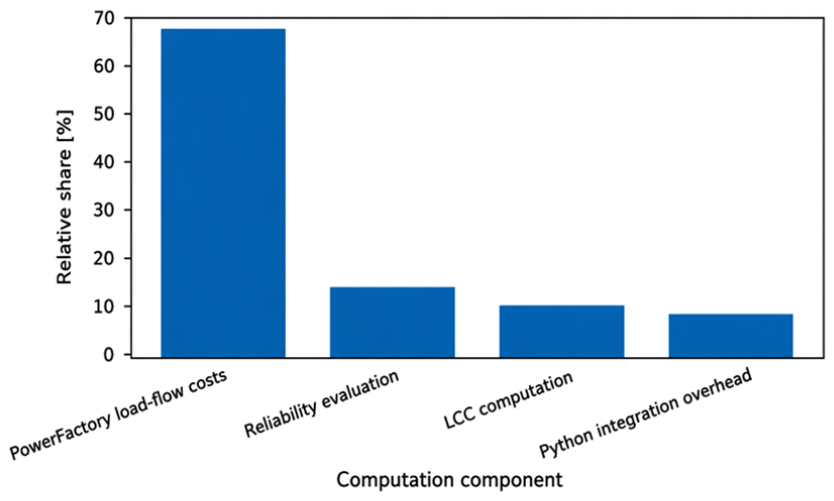
Scenario batching: for W_loss, the load scenarios are selected as a minimally sufficient set (typically 8–12 scenarios), and then expanded later in the sensitivity analysis. Figure 15 shows the distribution of the total computational time among the main components of the NSGA-II optimization process.

Reliability calculations (SAIDI/SAIFI), which are based on the network topology and consumer allocation, account for a smaller fraction of the total time. These results show that the most effective strategy for accelerating the optimization process is to reduce the number of PowerFactory calls or to apply parallel evaluation. Computational burden reduction strategies such as warm start, feasibility pre-check, parallel evaluation, and scenario batching were adopted in this study [18]. The computational complexity of the proposed framework is primarily dominated by repeated AC load-flow calculations performed within the DIgSILENT PowerFactory environment for each candidate solution. Therefore, the total execution time depends mainly on the population size, number of generations, and the number of evaluated operating scenarios. The proposed methodology is intended mainly for offline planning and design optimization rather than for real-time protection or millisecond-level operational control applications. Nevertheless, the framework can effectively support operational planning and long-term decision-making processes in modern urban distribution systems.

3. Results

3.1. Study Area, Network Boundary, and Source of Real Data

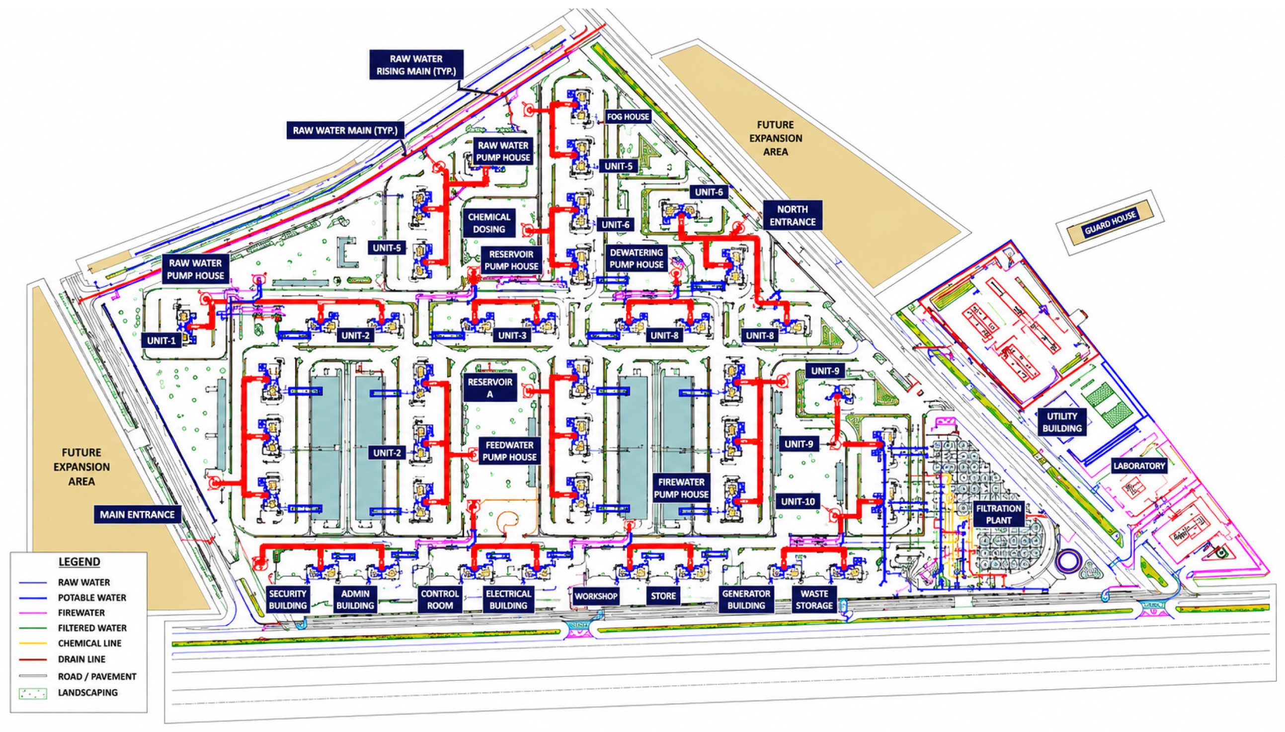
This case study focuses on the 0.4 kV low-voltage (LV) level of a 10/0.4 kV urban distribution system in Tashkent city. Area parameters (based on GIS data) (Figure 16):

• Total area: A = 0.48 km²;
• Building composition (segments):
• Ten+ storey residential buildings: 8 units;
• Five- to nine-storey residential buildings: 12 units;
• Commercial facilities: 3 units;
• Office buildings: 2 units.

This area model was used in the NSGA-II-based multi-objective optimization process to determine the optimal placement of TSs and to evaluate energy losses, LCC, and power supply reliability indices [12,21].

Real dataset (load profiles) and calibration: Based on the methodology presented in Section 2, the comfort coefficient (k_com) and the segment-specific load-shape parameters were calibrated using 4000 real 15 min load profiles (96 points per day).

Use of the dataset for reproducibility:

• In the optimization process, design-day and peak-day scenarios for each segment were generated from the real profiles using a bootstrap procedure (

  Table 11. Scenario set: 8–12 typical day scenarios by consumer segment (name, share, h_eq).

  Scenario ID	Scenario Name	Consumer Segment	Share (%)	Equivalent h heq	Description
  S1	Winter weekday peak	Residential	12	1050	Evening residential peak during heating season
  S2	Winter weekday off-peak	Residential	10	880	Night residential load
  S3	Winter commercial day	Commercial/Office	9	790	Daytime business activity
  S4	Summer HVAC peak	Residential + Office	14	1220	Cooling demand peak
  S5	Summer normal day	Mixed	11	960	Typical summer weekday
  S6	Weekend daytime	Residential/Commercial	13	1140	Weekend activity
  S7	Night base load	24/7 loads	10	880	Continuous operation facilities
  S8	Spring/autumn normal	Mixed	9	790	Mild season demand
  S9	Holiday reduced load	Mixed	5	440	Reduced activity days
  S10	Extreme peak day	All segments	4	350	95% quantile peak demand

  );
• In the calculation of losses and LCC, the annual equivalent energy loss (W_loss) was derived using scenario sets such as: (i) weekday, (ii) weekend, (iii) summer HVAC peak, and (iv) winter peak (Table 11) [31,32].

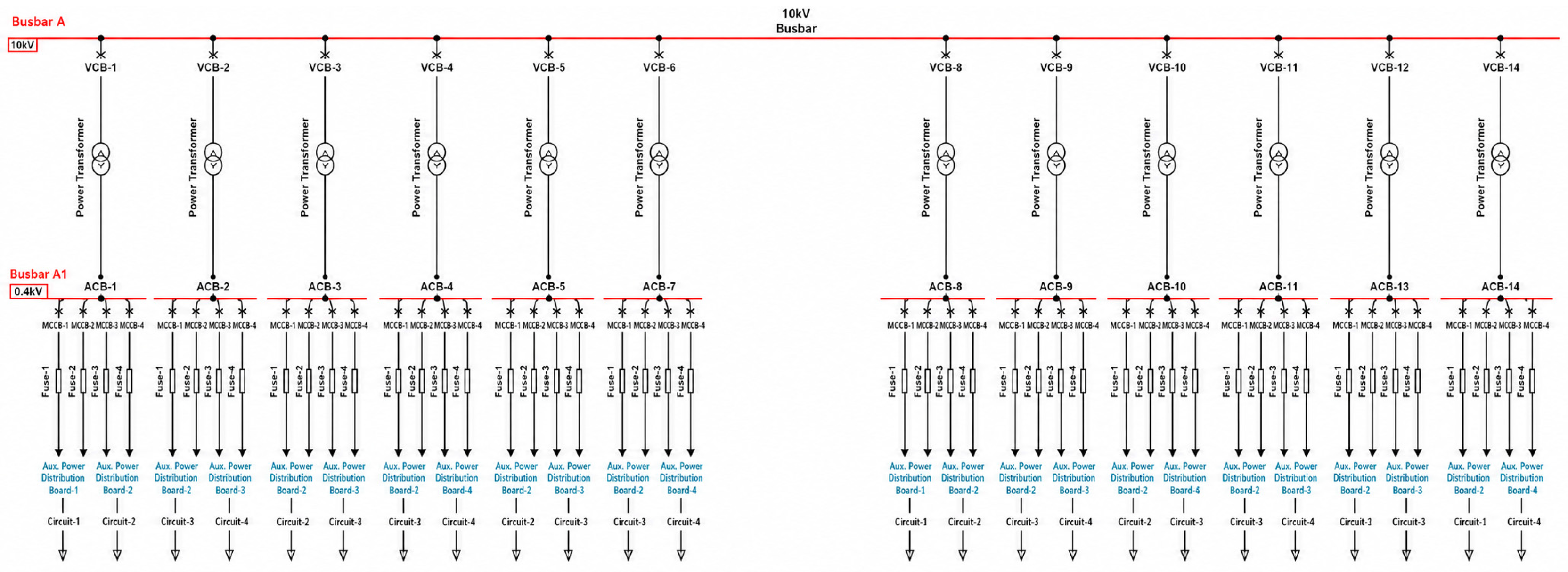
This scenario set makes it possible to convert network losses into an annual equivalent energy value [12,18,20,24,33]. Based on the initial data of the selected area, a model of the system was developed in DIgSILENT (Figure 17).

It can be observed that all electrical network parameters of the 12 TSs (TPs) located within the area are included.

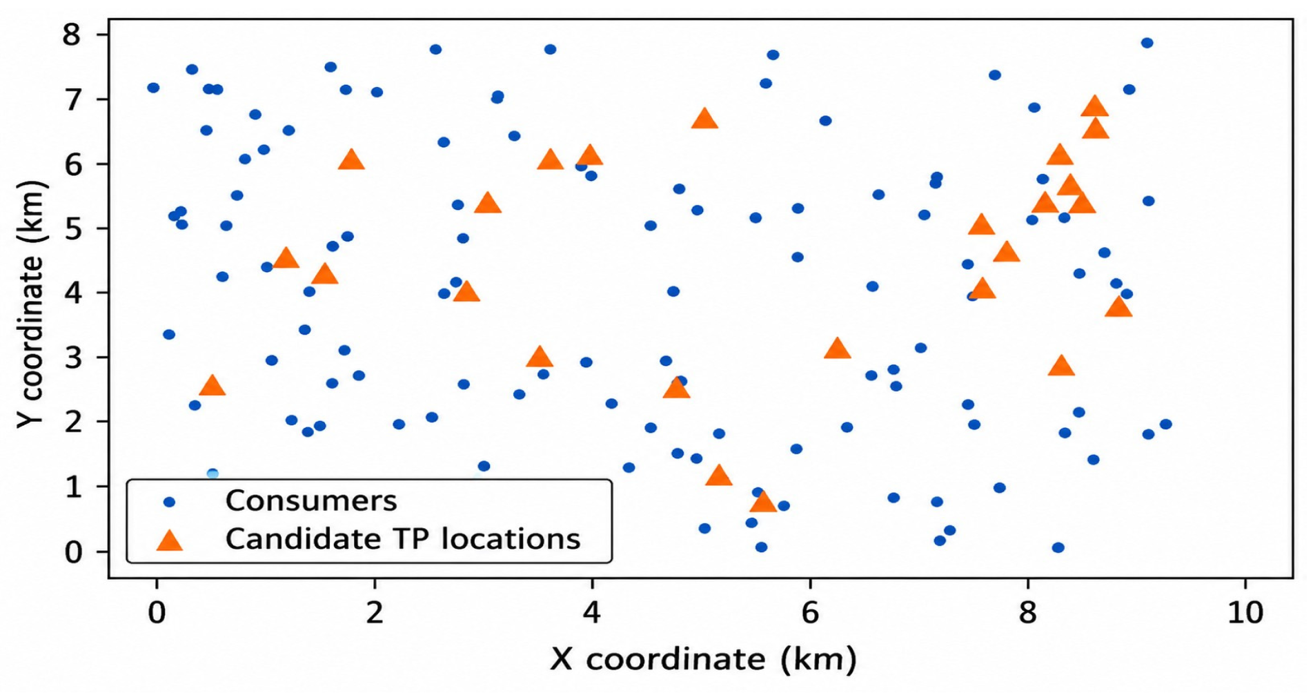
The consumer points represent residential, commercial, office, and continuously operating facilities, while the TS candidates are identified at locations consistent with the urban infrastructure and the existing utility corridors (Figure 18) [24,26].

In this way, the resulting network topology is constructed in a manner consistent with the real urban infrastructure [18,32,48].

3.2. Initial Load Model and Formation of the Design Peak

For each building type, the installed capacity and the corresponding coefficients were adopted as follows (

Table 12. Parameters by consumer segments: P_inst, k_dem, k_coin, k_com, cosφ.

Building Type	Pinst (kW)	kdem	kcoin	kcom
10+ storey buildings	180	0.6	0.85	1.25
5–9 storey buildings	120	0.6	0.8	1.15
Commercial buildings	250	0.75	0.9	1.20
Office buildings	200	0.7	0.85	1.18

) (the segmentation and calibration procedures are described in Section 2).

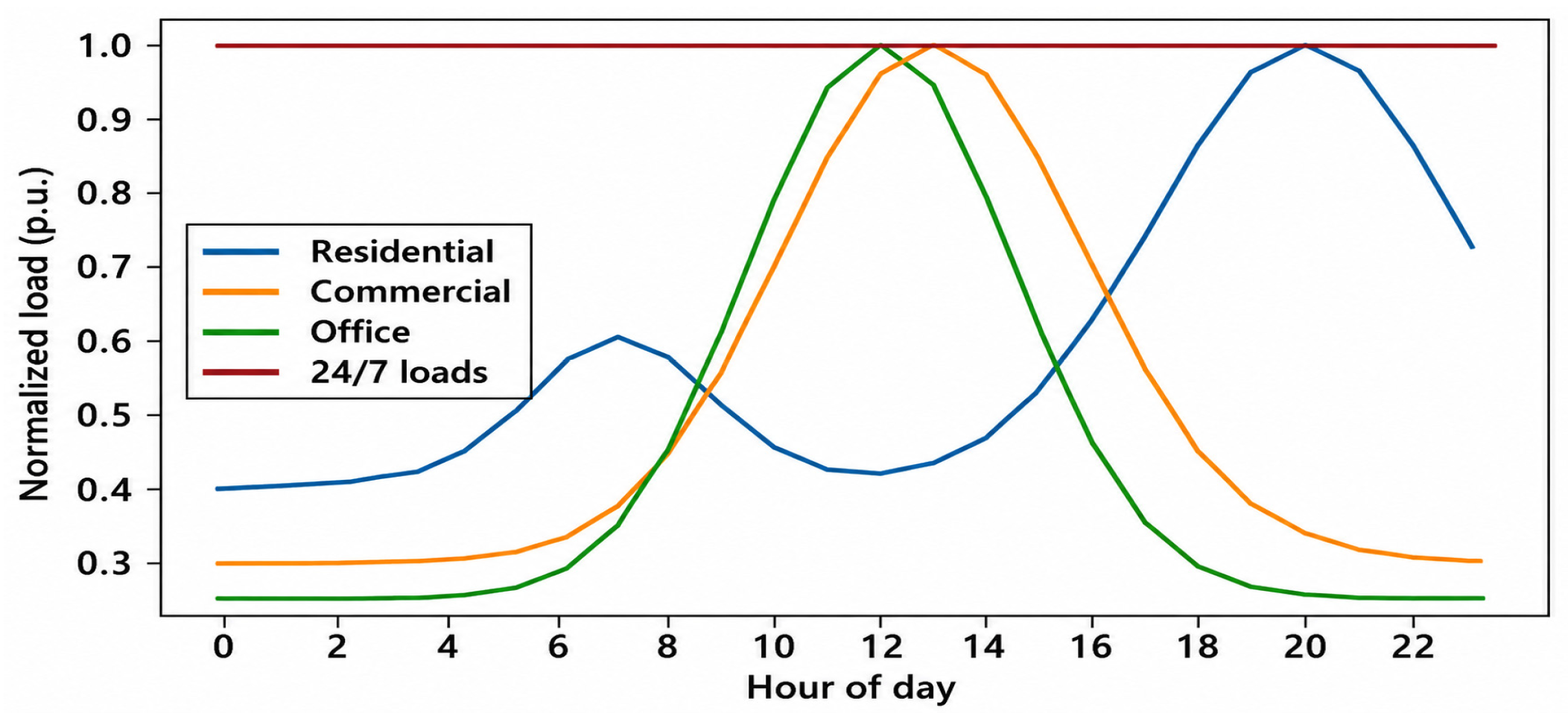
As a result of the calculation, the total active design load, obtained as the sum of all segments: P_des ≈ 3.18 MW. In a real LV topology, one TS typically supplies several feeders, and the load is distributed among phases. The current constraint in DIgSILENT was verified (Figure 19) [15,39]:

• At the feeder level;
• With phase balancing;
• While accounting for segment-wise diversification based on daily load profiles.

The graph illustrates the normalized load dynamics for residential, commercial, office, and continuously operating (24/7) facilities. These segment-specific load patterns allow the optimization model to account for the diversification effect in electricity demand and enable the design load to better reflect the real consumption structure of urban distribution networks [46].

3.3. Transformer Selection and the Number of Substations

Two typical transformer capacity options were compared: 250 kVA and 400 kVA transformers. For operational safety, the loading coefficient was adopted as: k_load = 0.75

For the 400 kVA transformer:

$$S_{\mathit{op}}=0.75 · 400 = 300 \mathrm{kVA}$$

(66)

$$P_{\mathit{TS}}^{\mathit{max}}=S_{\mathit{op}}·\mathit{cos}\phi =300 · 0.92=276 \mathrm{kW}$$

(67)

$$N_{\mathit{TS}}=⌈{\displaystyle \frac{P_{\mathrm{h}\mathit{is}}}{P_{\mathit{TS}}^{\mathit{max}}}}⌉=⌈{\displaystyle \frac{3180}{276}}⌉=12$$

(68)

In the 250 kVA option, the required number of TSs approaches 18, which:

• Increases capital expenditure;
• Makes implementation more difficult because of urban space constraints;
• Leads to greater complexity due to the larger number of substations.

The main optimization was carried out for a configuration based on 12 TSs rated at 400 kVA each (

Table 13. Technical and planning comparison of 250 kVA and 400 kVA transformer substation options.

Indicator	250 kVA option	400 kVA Option (Selected)	Comment/Design Implication
Rated capacity, Snom (kVA)	250	400	Standard TS ratings
Operating loading coefficient, kload	0.75	0.75	Adopted for thermal safety and reserve margin
Operating apparent power, Sop = kload·Snom (kVA)	187.5	300
Power coefficient, cosφ	0.92	0.92	Assumed for urban LV segments
Operating active power limit, PTSmax = Sop·cosφ (kW)	172.5	276
Total design load, Pdes (kW)	3180	3180	Sum of all consumer segments
Required number of TSs, NTS = [Pdes/PTSmax]	[3180/172.5] = 19	[3180/276] = 12	For 250 kVA, the practical requirement is around 18–19 depending on planning reserve
Impact of TS number under urban space constraints	Higher burden (more sites required)	Lower burden (fewer sites required)	Site availability and permitting are critical in urban areas
O&M complexity (relay, protection, maintenance)	Higher	Lower	As the number of TSs increases, service cost and the number of possible failure points also increase
Estimated TS CAPEX (TS equipment only)	CAPEXTS = NTS·C250	CAPEXTS = NTS·C400	Here, C250 and C400 are the unit costs of one TS
CAPEX difference (parametric)	∆CAPEX = 19C250-12C400	—	Once real market prices are inserted, the difference can be obtained directly
LV feeder length (trend)	Shorter average feeders, but a larger number of feeders	Longer average feeders, but fewer feeders	Increasing the number of TSs reduces the radius; reducing the number of TSs increases it
Trend in losses and voltage quality	Losses ↓, ∆U ↓	Losses ↑, ∆U ↑	The optimal radius is then identified through the NSGA-II trade-off analysis
Trend in reliability (SAIDI)	SAIDI ↓ due to shorter feeders	SAIDI ↑ due to longer feeders	For this reason, SAIDI is included as an objective in the model

Note: “—” indicates that the corresponding value is not applicable; “↑” and “↓” indicate an expected increase and decrease, respectively, in the corresponding performance indicator.

).

In contrast, for the 250 kVA option, =172.5 kW, and the required number of substations approaches 18–19, which is practically less favorable in urban areas due to site availability constraints, greater implementation and permitting complexity, and increased burden. The optimization and Pareto analysis are carried out for a configuration consisting of 12 TSs rated at 400 kVA, while the service radius R is determined by NSGA-II on the basis of the trade-off among losses, reliability, and cost [12,15,21].

3.4. Cable Parameters and LV Line Model

In the optimization process, two practical cable cross-sections were considered for the 0.4 kV network (

Table 14. Cable cross-sections: r′ and I_allow.

Cross-Section	r′ (Ohm/km)	Iallow (A)
95 mm2	0.193	260
120 mm2	0.153	300

).

The main trade-off considered here is:

• For 120 mm²: smaller service radius R → lower I²·R losses, but higher CAPEX;
• For 95 mm²: lower CAPEX, but higher losses and more noticeable voltage drop.

The cable cross-section was also included in the sensitivity analysis. In addition to cable cross-sectional optimization, transformer capacity was also analyzed within the sensitivity analysis framework. The results demonstrated that increasing transformer capacity reduced overload probability and voltage deviations; however, excessive transformer sizing increased the overall life-cycle cost of the system. Sensitivity analysis further showed that transformer capacity selection strongly depends on urban load density and operational constraints.

3.5. Defining the Service Radius R as a Theoretical Upper Bound and Its Role in Optimization

The service radius R is introduced as a decision variable (consistent with Section 4).

From theoretical assessment, the permissible range was estimated as:

• For a 95 mm² cable: R ≈ 250–300 m;
• For a 120 mm² cable: R ≈ 300–350 m.

For the NSGA-II optimization, the search space was defined as: R ∈ [250, 350] m

In a real distribution system:

• The load is distributed among several feeders;
• Phase balancing is applied;
• Line-end currents typically remain within 200–300 A, depending on cable cross-section and network topology.

The current constraint was not evaluated using simplified analytical approximations, but was instead rigorously verified using PowerFactory AC load-flow calculations [35].

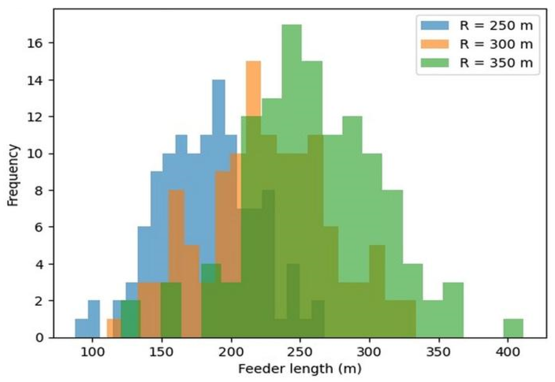
The Figure 20 shows how increasing the admissible service radius shifts the feeder length distribution toward longer LV feeders, which directly affects power losses, voltage drop, and reliability.

3.6. Reliability Parameters and the SAIDI Model

In the reliability analysis, the following normative/statistical parameters were adopted:

• Failure rate: λ₀ = 0.25 (interruptions/km·year);
• Average restoration time: r = 3 h.

The failure rate of an LV line is assumed to be proportional to its length: λ_l = λ₀·L_l.

$$\mathit{SAIDI}\left(X\right)={\displaystyle \frac{\sum _k{U}_k\left(X\right)N_k\left(X\right)}{N_{\mathit{tot}}}}$$

(69)

SAIDI cannot be represented solely by the simplified expression λ·r, instead, it is recalculated using the network topology and consumer assignment results obtained from the PowerFactory model [12,32,36]. Reliability model input parameters for the urban LV distribution network, including feeder failure intensity, repair time, customer composition, and critical load share (

Table 15. Reliability inputs: λ₀, r, number/share of consumers by segment, and share of critical loads.

Parameter	Symbol	Value	Unit	Description
Base failure intensity	λ0	0.25	outages/km·year	LV feeder failure rate
Average repair time	r	3	h	Mean outage restoration time
Residential customer share	–	0.55	–	Share of residential consumers
Commercial customer share	–	0.20	–	Share of commercial consumers
Office customer share	–	0.15	–	Share of office consumers
Critical load share	–	0.10	–	Share of 24/7 or critical loads

).

3.7. NSGA-II Results: Pareto Front and Representative Solutions

The optimization was carried out using the NSGA-II algorithm integrated with DIgSILENT PowerFactory in an in-the-loop framework:

• TS placement;
• Service radius R;
• Load-flow results (U_i, I_l, P_loss);
• Objective indicators: C_LCC, W_loss, and SAIDI;
• Constraint violation measure CV(X).

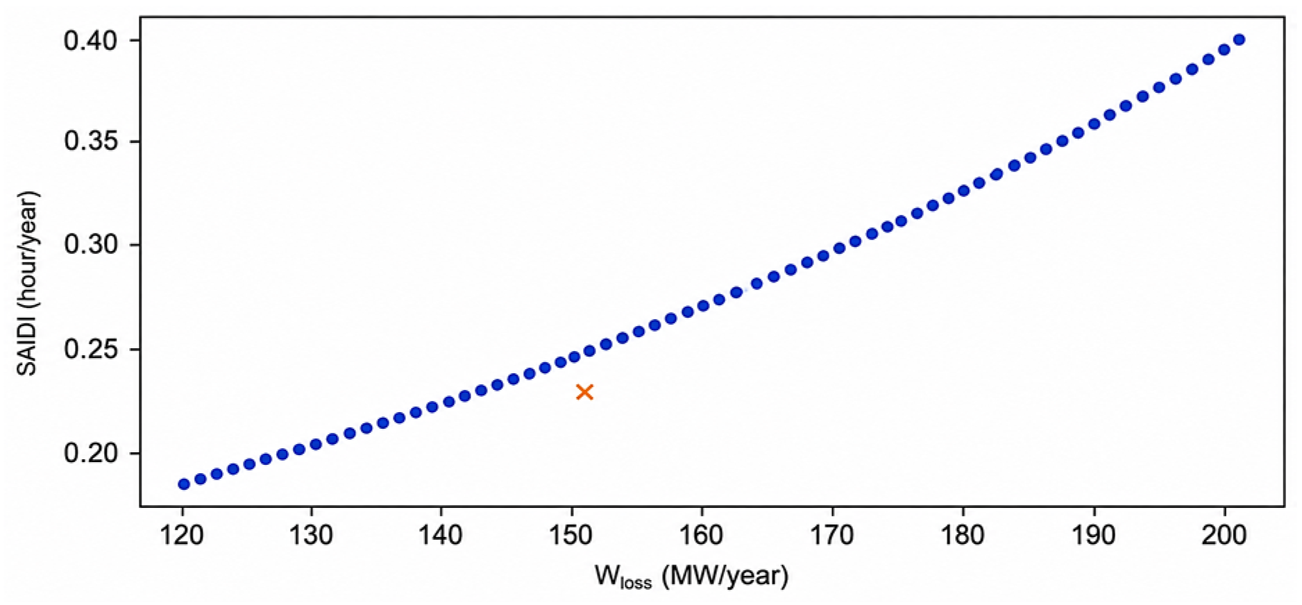
A set of Pareto-optimal solutions was obtained. From this set, the knee-point solution representing the most balanced compromise among the objectives was selected.

Each point represents a feasible network configuration; lower-left solutions indicate better technical performance, while the color-coded C_LCC contour can be added in the final journal version (Figure 21).

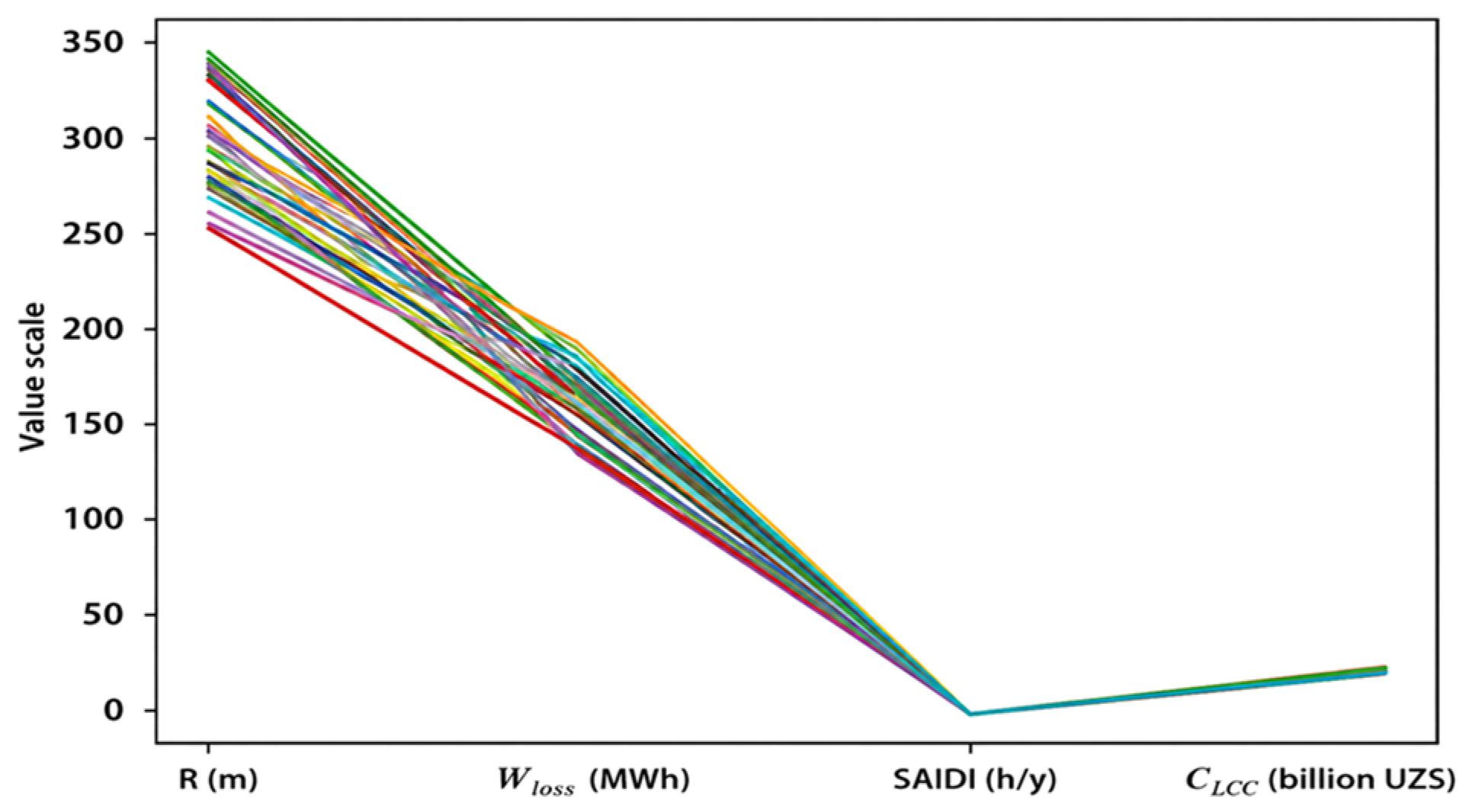
Parallel coordinate representation of NSGA-II solutions across (Figure 22) the main decision and performance variables: service radius R, annual energy losses W_loss, reliability index SAIDI, and LCC C_LCC.

Representative Pareto solutions with respect to radius R.

These solutions are chosen to illustrate the impact of R on power losses (W_loss), reliability (SAIDI), and life cycle cost (C_LCC) (

Table 16. Representative solutions: losses, SAIDI, and C_LCC as a function of R.

Radius R	Ploss (kW)	SAIDI (h/Year)	CLCC (Billion UZS)
250 m	128	0.19	21.6
300 m	142	0.23	20.8
350 m	176	0.28	20.4

) [25,41]:

A clear trade-off is observed in this context:

• Small R → shorter feeders → lower power losses and improved SAIDI, but higher CAPEX/LCC;
• Large R → wider transformer service areas → increased losses and worse SAIDI, but reduced capital cost.

4. Discussion

4.1. Sensitivity Analysis: R, Cable Cross-Section, Discount Rate, Tariff, and k_com

The sensitivity analysis is not limited to the service radius R only; four main parameter groups are considered.

4.1.1. Sensitivity with Respect to R = {250, 300, 350}

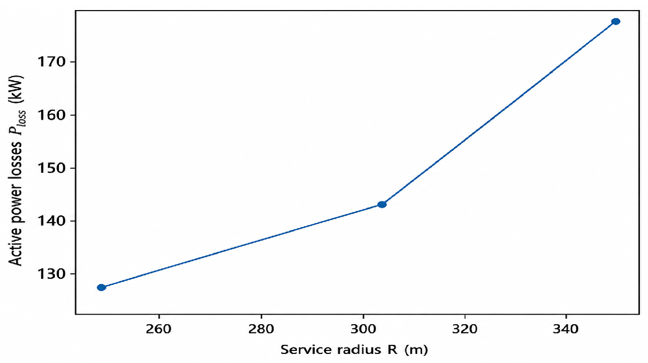
Technical impact: Power losses increase with R due to the I²·R nature of line losses.

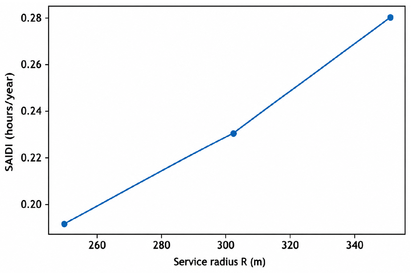
Reliability impact: SAIDI increases from 0.19 to 0.28 h/year (about 47% increase), reflecting the larger affected area per outage as feeder lengths grow.

However, this comes at the expense of higher energy losses and degraded service quality, leading to a trade-off between CAPEX savings and operational performance [12,18,26,37].

As the radius increases, the feeder length also increases, and the losses rise according to the I²·R nature of electrical networks. Increasing the radius from R = 250 m to R = 350 m leads to an about 37% increase in losses, which confirms the necessity of optimizing the service radius (Figure 23).

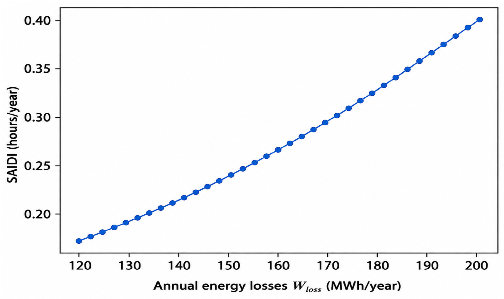
According to the results, when the radius increases from R = 250 m to R = 350 m, the SAIDI value rises from 0.19 to 0.28 h/year (Figure 24).

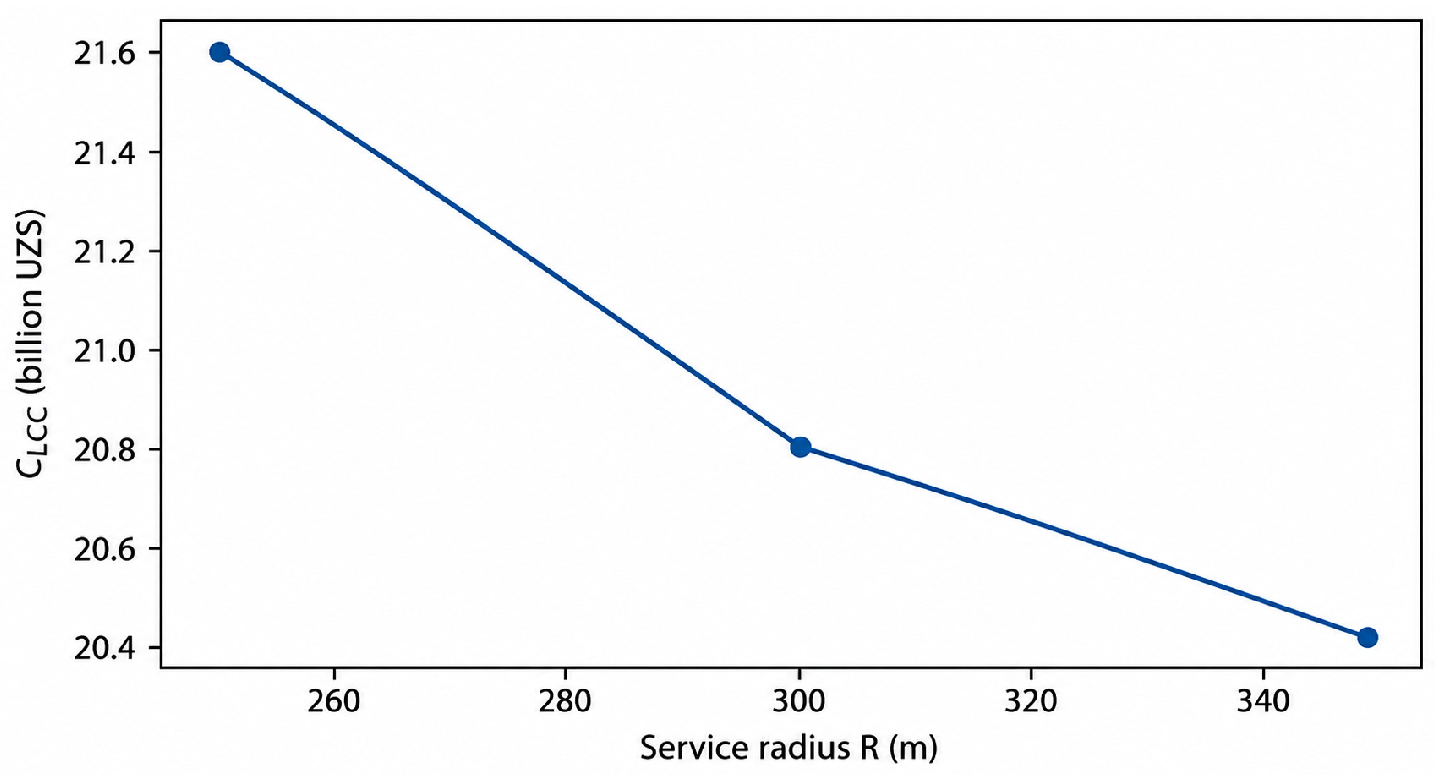
However, energy losses increase, leading to higher operating expenditures (Figure 25) [9,13,18,25].

4.1.2. Sensitivity with Respect to Cable Cross-Section

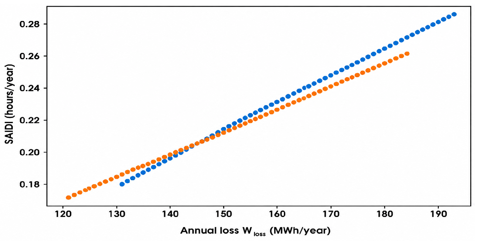
For each value of R, the 95 and 120 mm² cable options are optimized separately and their Pareto fronts are compared (Figure 26):

• 120 mm² reduces losses and improves the voltage profile;
• 95 mm² lowers CAPEX, but when R is large, the risk of constraint violation increases.

A 120 mm² cable reduces electrical resistance, which leads to lower power losses and improved voltage profiles.

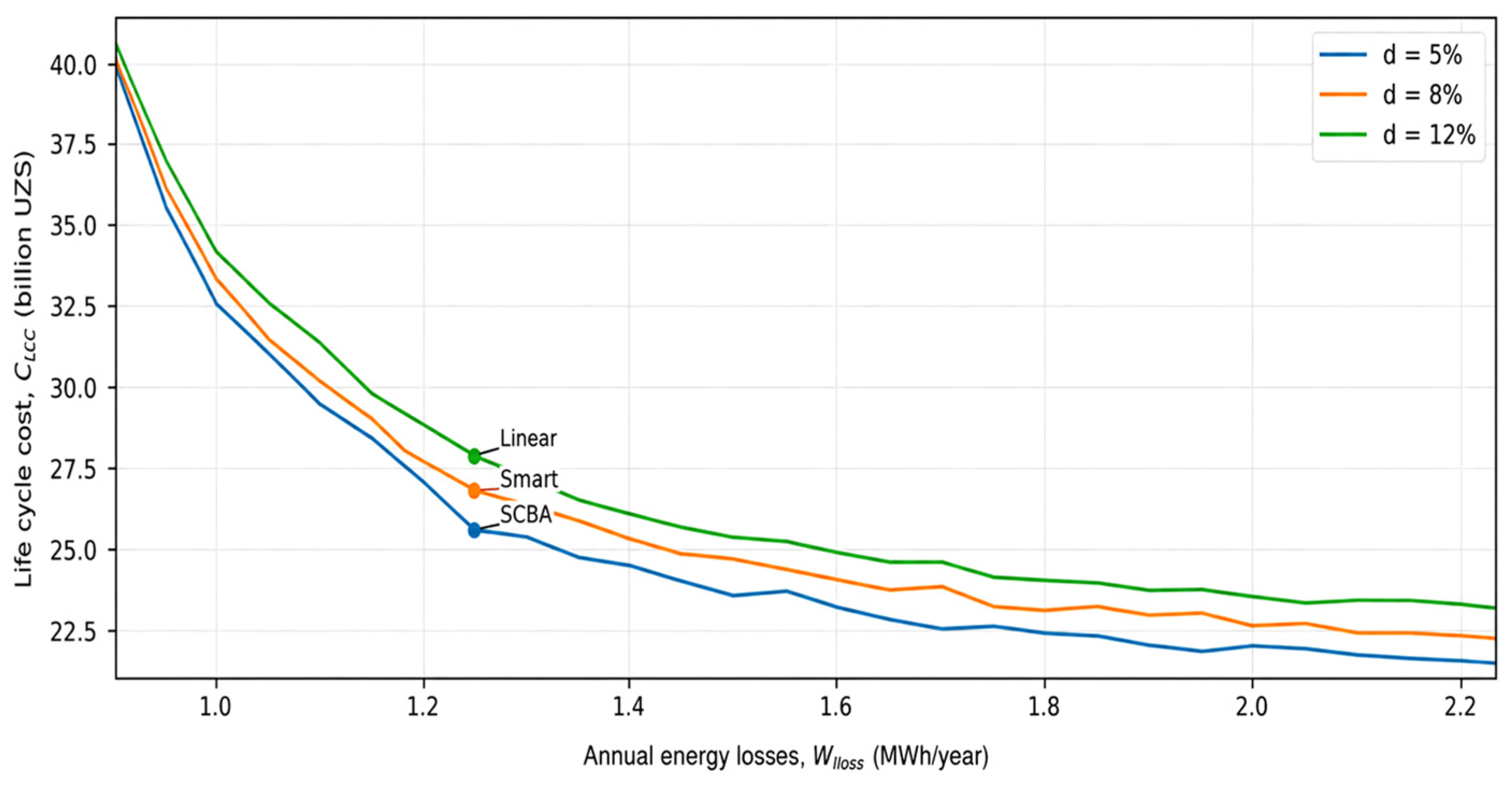
4.1.3. Sensitivity with Respect to Discount Rate d and Electricity Price c_e

The LCC, expressed in discounted terms, is highly sensitive to both the discount rate and the electricity tariff. The following scenarios are considered:

• d = {8%, 12%, 16%};
• C_e variation of ±20%.

Interpretation of results:

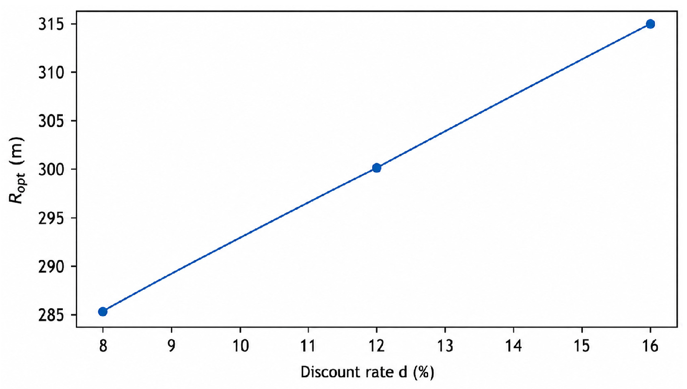
• As d increases, long-term losses become less significant in present value terms → capital cost dominates → the optimal R may shift toward larger values;
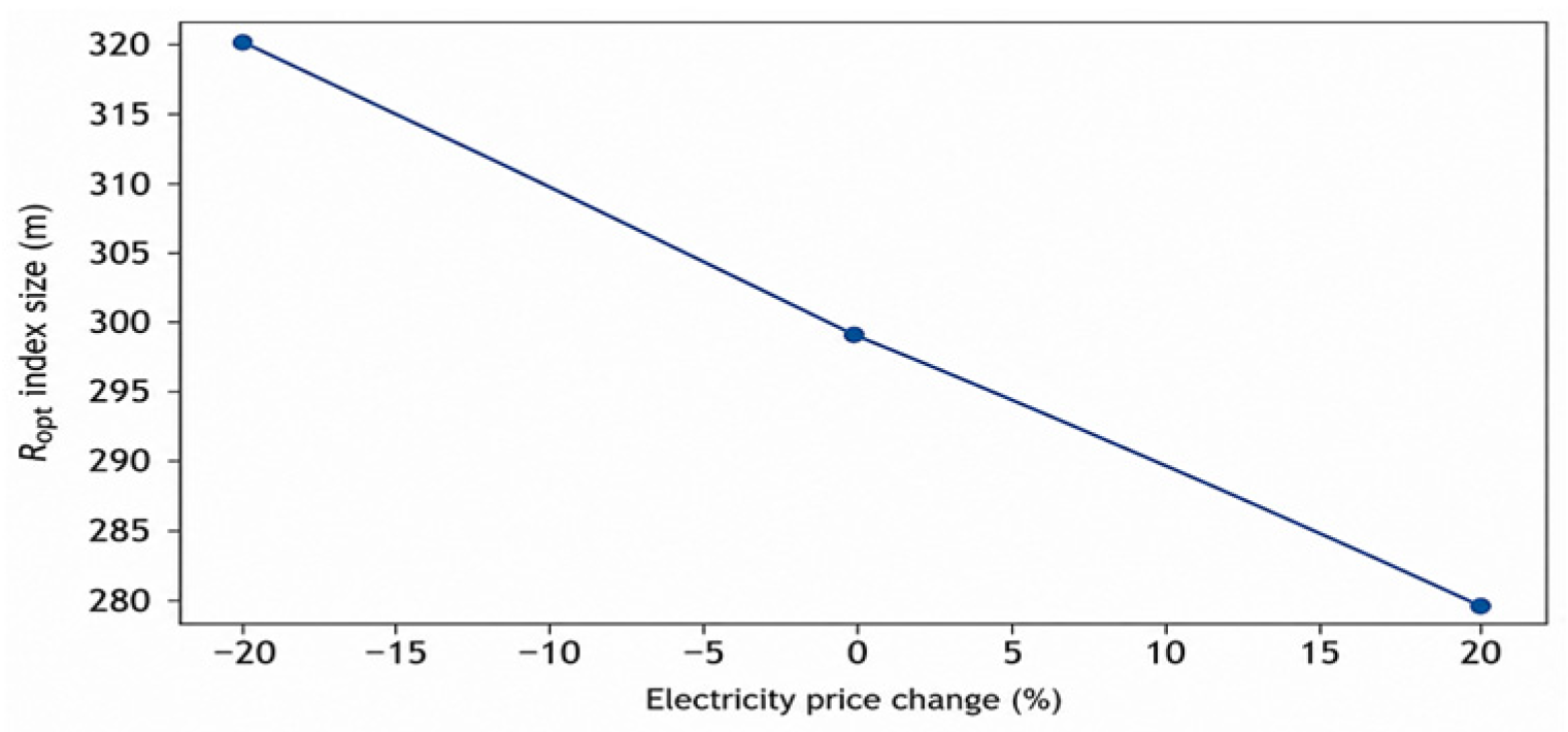
• As c_e increases, energy losses become more expensive → smaller R and/or larger cable cross-sections become more favorable.

As the discount rate increases, the present value of future energy losses decreases, making capital costs more dominant in the decision-making process. The optimization tends to favor solutions with larger service radius (Figure 27).

As the electricity price increases, the economic value of power losses also increases. The optimization algorithm typically prefers smaller radii and configurations with lower losses (Figure 28).

4.1.4. Ablation Study on k_com

What kind of error does the optimization produce when the “comfort coefficient” is removed (

Table 17. Ablation summary: CV, P_loss, SAIDI, C_LCC for Case A vs. Case B.

Case	kcom	Constraint Violation CV	Wloss (MWh)	SAIDI (h/y)	CLCC (bln UZS)
Case A	1.0	0.12	178	0.31	20.1
Case B	data-driven	0.00	142	0.23	20.8

) [7,12,14,47]:

• Case A: k_com = 1 (classical normative model);
• Case B: data-driven k_com (proposed model);
• Expected and demonstrated result;
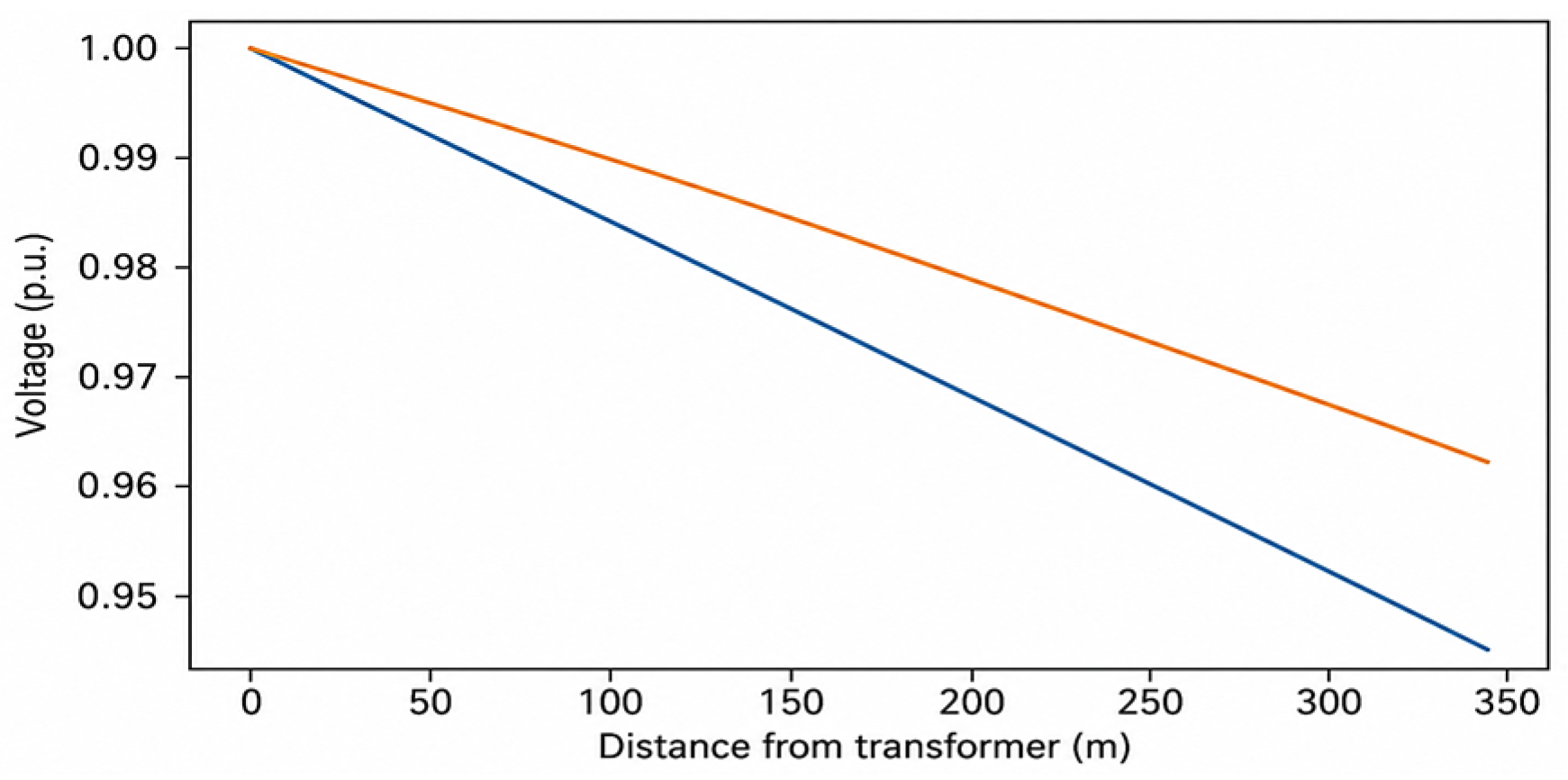
• Case A usually underestimates the load → transformer placement and radius selection become overly “optimistic” → voltage constraints/thermal constraints are more frequently violated, or SAIDI worsens in real operation.

The voltage profiles for the fixed and data-driven comfort coefficient cases are compared in Figure 29.

This result shows that incorporating the comfort coefficient into the model improves the accuracy of electrical network design.

4.2. Selection of the Optimal Variant: Pareto Knee-Point and Practical Decision

In a multi-objective problem, there is no single “best” solution; a practical decision is typically made using the knee-point (compromise solution). The knee-point was selected based on the following criteria [5,12,18,26,41]:

• Full satisfaction of constraints (CV = 0);
• Before the point where SAIDI and power losses begin to increase sharply;
• C_LCC close to its minimum value.

As a result: R_opt ≈ 300 m.

This solution:

• Does not violate voltage constraints;
• Does not exceed thermal current limits;
• Provides acceptable SAIDI;
• Offers a near-minimum C_LCC compromise.

The knee-point solution selected from the Pareto front is shown in Figure 30.

This result shows that incorporating the comfort coefficient into the model improves the accuracy of electrical network design. It can be observed that, as a result of applying the conducted research and obtained results to the real object, the values shown in Figure 31 were achieved [14].

4.3. Interpretation of the Results from Technical, Economic, and Reliability Perspectives

The results show that, in urban LV networks, the service radius R is not merely a geometric parameter, but rather a design lever that governs the following three aspects. Energy efficiency: as R increases, feeders become longer, which leads to higher I²·R losses. Service quality (reliability): as LV line length increases, the failure rate also increases and the outage impact area expands. The increase in SAIDI is driven not only by λL, but is further amplified by assignment and topology. Economic efficiency (LCC): a larger R generally allows less dense placement of TSs and reduces capital requirements. The solution around 300 m provides a balanced compromise among technical, economic, and reliability criteria under urban conditions. The results also indicate that increasing the service radius leads to longer feeder lengths, which, according to the I²·R law, causes a quadratic increase in power losses. Greater network length raises the probability of interruption and contributes to a deterioration in the SAIDI index.

5. Conclusions

This study investigated the problem of transformer substation placement in urban 10/0.4 kV distribution networks using an integrated multi-objective optimization framework combining technical, economic, and reliability criteria. The increasing complexity of urban electricity consumption, particularly due to the expansion of HVAC systems and electric vehicle charging infrastructure, demonstrated the limitations of traditional empirical planning approaches. Therefore, the planning problem was formulated as a Pareto-based multi-objective optimization task and solved using the NSGA-II algorithm integrated with DIgSILENT PowerFactory AC load-flow simulations.

The results demonstrated that the service radius is a critical strategic parameter affecting energy losses, life-cycle cost, and reliability performance in urban distribution systems. Pareto-front analysis showed that a service radius of approximately 300 m provides the most balanced compromise between technical, economic, and reliability objectives under the investigated operating conditions. For the studied 0.48 km² urban area in Tashkent city with a total load demand of 3.18 MW, the optimized configuration consisted of 12 transformer substations based on 400 kVA transformers.

The proposed comfort-coefficient-based urban load model indicated that the actual maximum demand may exceed the normative estimate by approximately 15–25%, thereby improving the accuracy of transformer sizing and load-density assessment. Sensitivity analysis within the 250–350 m service-radius range showed that increasing the radius leads to higher power losses and reduced reliability performance, although capital investment costs decrease.

The main scientific contributions of the study are as follows:

• an urban load model incorporating the comfort coefficient was developed;
• a multi-objective C_LCC–P_loss–SAIDI optimization model was formulated;
• an NSGA-II-based Pareto planning framework for urban transformer substation placement was proposed.

The integration of NSGA-II with AC load-flow simulation enabled stable Pareto-front generation and effective solution of the constrained nonlinear optimization problem. Although the proposed methodology is generally applicable to urban distribution systems, the comfort coefficient values should be regionally calibrated to account for local climatic conditions, infrastructure characteristics, and consumer behavior patterns.

References

1. International Energy Agency (IEA). Electricity 2024: Analysis and Forecast to 2026; IEA: Paris, France, 2024; Available online: https://www.iea.org/reports/electricity-2024 (accessed on 1 April 2026).
2. United Nations Department of Economic and Social Affairs (UN DESA). World Urbanization Prospects 2023 Revision; United Nations Department of Economic and Social Affairs (UN DESA): New York, NY, USA, 2023. [Google Scholar]
3. International Energy Agency (IEA). Global EV Outlook 2024; IEA: Paris, France, 2024; Available online: https://www.iea.org/reports/global-ev-outlook-2024 (accessed on 1 April 2026).
4. Melikuziev, M.V. Determination of the service area and location of transformer substations in the city power supply system. E3S Web Conf. 2023, 384, 01033. [Google Scholar] [CrossRef]
5. Lund, H. Renewable energy strategies for sustainable development. Energy 2007, 32, 912–919. [Google Scholar] [CrossRef]
6. Sultana, S.; Roy, P.K. Multi-objective quasi-oppositional teaching-learning-based optimization for optimal location of distributed generator in radial distribution systems. Int. J. Electr. Power Energy Syst. 2014, 63, 534–545. [Google Scholar] [CrossRef]
7. Rajalakshmi, J.; Durairaj, S. Review on optimal distributed generation placement using particle swarm optimization algorithms. In Proceedings of the 2016 International Conference on Emerging Trends in Engineering, Technology and Science (ICETETS), Pudukkottai, India, 24–26 February 2016; IEEE: Piscataway, NJ, USA, 2016; Volume 4, pp. 1–6. Available online: https://ieeexplore.ieee.org/document/7603088 (accessed on 25 March 2026).
8. Qi, Q.; Wu, J.; Zhang, L.; Cheng, M. Multi-objective optimization of electrical distribution network operation considering reconfiguration and soft open points. Energy Procedia 2016, 103, 141–146. [Google Scholar] [CrossRef]
9. Kim, I. Optimal allocation of distributed generation and storage systems using multi-dimensional weighted least distance optimization and water droplet algorithms. Energy 2025, 320, 135371. [Google Scholar] [CrossRef]
10. Ramadhani, U.H.; Fachrizal, R.; Shepero, M.; Munkhammar, J.; Widén, J. Probabilistic load flow analysis of electric vehicle smart charging in unbalanced LV distribution systems with residential photovoltaic generation. Sustain. Cities Soc. 2021, 72, 103043. [Google Scholar] [CrossRef]
11. Al-Shaalan, A.M. Reliability evaluation of power systems. In Reliability and Maintenance—An Overview of Cases; Kounis, L., Ed.; IntechOpen: London, UK, 2019. [Google Scholar] [CrossRef]
12. DIgSILENT GmbH. PowerFactory Technical Reference Documentation; DIgSILENT GmbH: Gomaringen, Germany, 2022; Available online: https://www.digsilent.de (accessed on 13 March 2026).
13. Deb, K.; Pratap, A.; Agarwal, S.; Meyarivan, T. A fast and elitist multiobjective genetic algorithm: NSGA-II. IEEE Trans. Evol. Comput. 2002, 6, 182–197. [Google Scholar] [CrossRef]
14. Li, Y.; Wang, J.; Cao, Y. Multi-objective distributed robust cooperative optimization model of multiple integrated energy systems considering uncertainty of renewable energy and participation of electric vehicles. Sustain. Cities Soc. 2024, 104, 105308. [Google Scholar] [CrossRef]
15. Melikuziev, M.V.; Usmonaliev, S.; Khudoyberdiev, N.; Sodikov, J.; Imomaliev, Z. Issues of the design procedure for the power supply system. AIP Conf. Proc. 2024, 3152, 040031. [Google Scholar] [CrossRef]
16. Melikuziev, M.V.; Nematov, L.A.; Novikov, A.N.; Baymuratov, K.K. Technical and economic analysis of parameters of city distribution electric network up to 1000 V. E3S Web Conf. 2021, 289, 07016. [Google Scholar] [CrossRef]
17. Jing, L.; Guo, J.; Feng, T.; Han, L.; Zhou, Z.; Melikuziev, M. Research on energy optimization scheduling methods for systems with multiple microgrids in urban areas. In Proceedings of the 2024 IEEE 4th International Conference on Digital Twins and Parallel Intelligence (DTPI); IEEE: Piscataway, NJ, USA, 2024; Volume 7, pp. 706–711. [Google Scholar] [CrossRef]
18. Melikuziev, M.V.; Fayzrakhmanova, Z.; Akhmedov, A.; Kasimova, G. Development of an educational simulator’s working logic for the course “Fundamentals of Power Supply”. AIP Conf. Proc. 2024, 3152, 050025. [Google Scholar] [CrossRef]
19. Wang, C.; Wu, J.; Ekanayake, J.; Jenkins, N. Planning of smart distribution systems. In Smart Electricity Distribution Networks; CRC Press: Boca Raton, FL, USA, 2017. [Google Scholar] [CrossRef]
20. Bhattacharjee, T.; Rajeshwari, M.; Kumar, K.J. Electric vehicle charging and its effects on the power distribution network. Power Res.—J. CPRI 2024, 20, 89–98. [Google Scholar] [CrossRef]
21. Zhou, G.; Bai, M.; Li, H.; Li, J.; Li, Q.; Liu, J.; Yu, D. Multi-objective station-network synergy planning for regional integrated energy system considering energy cascade utilization and uncertainty. Energy Convers. Manag. 2024, 301, 118073. [Google Scholar] [CrossRef]
22. Roman-Messina, A. Power system stability and control. In Standard Handbook for Electrical Engineers, 17th ed.; Santoso, S., Beaty, H.W., Eds.; McGraw-Hill: New York, NY, USA, 2018; Volume 28, pp. 1239–1327. [Google Scholar]
23. Baran, M.E.; Wu, F.F. Optimal capacitor placement on radial distribution systems. IEEE Trans. Power Deliv. 1989, 4, 725–734. [Google Scholar] [CrossRef]
24. Baran, M.E.; Wu, F.F. Network reconfiguration in distribution systems for loss reduction and load balancing. IEEE Trans. Power Deliv. 1989, 4, 1401–1407. [Google Scholar] [CrossRef]
25. Kennedy, J.; Eberhart, R. Particle swarm optimization. In Proceedings of the 1995 IEEE International Conference on Neural Networks (ICNN), Perth, Australia, 27 November–1 December 1995; IEEE: Piscataway, NJ, USA, 1995; Volume 4, pp. 1942–1948. [Google Scholar] [CrossRef]
26. Gromovyy, O.; Smail, A.; Smagulova, K.; Melikuziev, M.; Baranovska, M.; Romanets, A.; Novitsky, I.; Humeniuk, A.; Kolysnychenko, I.; Bilukhin, D. Determination of electricity quality indicators in distribution networks of industrial enterprises when using starting devices of powerful electric drives. Technol. Audit. Prod. Reserves 2025, 1, 57–64. [Google Scholar] [CrossRef]
27. Dorigo, M.; Birattari, M.; Stützle, T. Ant colony optimization. IEEE Comput. Intell. Mag. 2006, 1, 28–39. [Google Scholar] [CrossRef]
28. Farhangi, H. The path of the smart grid. IEEE Power Energy Mag. 2010, 8, 18–28. [Google Scholar] [CrossRef]
29. Mehta, P.; Bhatt, P.; Pandya, V. Optimal selection of distributed generating units and its placement for voltage stability enhancement and energy loss minimization. Ain Shams Eng. J. 2018, 9, 187–201. [Google Scholar] [CrossRef]
30. Ferraz, R.S.F.; Júnior, V.F.S.; Rueda-Medina, A.C. Multi-objective approach for distribution system planning considering stochastic customer-owned distributed energy resources. IEEE Access 2025, 13, 40561–40576. [Google Scholar] [CrossRef]
31. Strbac, G. Demand side management. Energy Policy 2008, 36, 4419–4426. [Google Scholar] [CrossRef]
32. Sun, S.; Yu, P.; Xing, J.; Wang, Y.; Yang, S. Multi-objective collaborative optimization of active distribution network operation based on improved particle swarm optimization algorithm. Sci. Rep. 2025, 15, 8999. [Google Scholar] [CrossRef]
33. Umoru, I.A.; Amhenrior, H.; Kenechi, A.V.; Makanju, T. Voltage profile improvement in distribution network under maximum loading (a case study). J. Multidiscip. Eng. Sci. Technol. 2023, 10, 16317–16324. [Google Scholar]
34. Huda, A.S.N.; Živanović, R. Large-scale integration of distributed generation into distribution networks: Study objectives, review of models and computational tools. Renew. Sustain. Energy Rev. 2017, 76, 974–988. [Google Scholar] [CrossRef]
35. Mirjalili, S.; Mirjalili, S.M.; Lewis, A. Grey wolf optimizer. Adv. Eng. Softw. 2014, 69, 46–61. [Google Scholar] [CrossRef]
36. Pinzón, S.; Yánez, S.; Ruiz, M. Optimal location of transformers in electrical distribution networks using geographic information systems. Enfoque UTE 2020, 11, 84–95. [Google Scholar] [CrossRef]
37. Malika, B.K.; Pattanaik, V.; Panda, S.; Rout, P.K.; Sahu, B.K.; Bajaj, M.; Blazek, V.; Prokop, L. A critical review of distribution system planning: Optimal placement and sizing of distributed generation and energy storage devices in microgrids. Energy Strategy Rev. 2025, 62, 101947. [Google Scholar] [CrossRef]
38. Mohammadi, A.; Kargarian, A. Momentum extrapolation prediction-based asynchronous distributed optimization for power systems. Electr. Power Syst. Res. 2021, 196, 107193. [Google Scholar] [CrossRef]
39. Ageev, V.A.; Dushutin, K.A.; Kazakov, D.V.; Golobokov, S.V. Approach to determining the power and location of transformer substations. In Proceedings of the 2022 4th International Youth Conference on Radio Electronics, Electrical and Power Engineering (REEPE); IEEE: Piscataway, NJ, USA, 2022. [Google Scholar] [CrossRef]
40. Yang, X.-S. Nature-Inspired Optimization Algorithms, 2nd ed.; Academic Press: Cambridge, MA, USA, 2021. [Google Scholar]
41. Alipour, M.A.; Askarzadeh, A. An efficient optimization framework for distribution network planning by simultaneous allocation of photovoltaic distributed generations and transformers. IET Renew. Power Gener. 2024, 18, 153–168. [Google Scholar] [CrossRef]
42. Shi, P.; Li, Y.; Du, Y.; Cai, Q.; Chen, H. Distribution network planning considering uncertainty of incremental distribution network access. In Proceedings of the 2020 IEEE 4th Conference on Energy Internet and Energy System Integration (EI2); IEEE: Piscataway, NJ, USA, 2020; Available online: https://ieeexplore.ieee.org/document/9347026 (accessed on 14 March 2026).
43. Gazijahani, F.S.; Salehi, J. Reliability constrained two-stage optimization of multiple renewable-based microgrids incorporating critical energy peak pricing demand response program using robust optimization approach. Energy 2018, 161, 999–1015. [Google Scholar] [CrossRef]
44. IEEE Standards Association (IEEE SA). The IEEE Standards Association—Home. Available online: https://standards.ieee.org/ (accessed on 28 March 2026).
45. Moradi, M.; Abedini, M. A combination of genetic algorithm and particle swarm optimization for optimal DG location and sizing in distribution systems. Int. J. Electr. Power Energy Syst. 2012, 34, 66–74. [Google Scholar] [CrossRef]
46. Saldaña-Gonzalez, A.; Ragüés-Peñalba, M.; Sumper, A.; Can-Taştan, I.; Gazioğlu, I. Distribution network planning considering EV integration: Case study in the northwest of Turkey. In Proceedings of theCIRED Porto Workshop 2022: E-Mobility and Power Distribution Systems, Porto, Portugal, 2–3 June 2022; Volume 7, pp. 945–949. [Google Scholar] [CrossRef]
47. Adinolfi, G.; Ciavarella, R.; Graditi, G.; Ricca, A.; Valenti, M. Innovative method for reliability assessment of power systems: From components modeling to key indicators evaluation. Electronics 2024, 13, 275. [Google Scholar] [CrossRef]
48. Korunovic, L.; Stojanovic, D. Load modeling for distribution networks. Facta Univ. Ser. Electron. Energetics 2002, 15, 419–427. [Google Scholar] [CrossRef]
49. Fekri, M.N.; Patel, H.; Grolinger, K.; Sharma, V. Deep learning for load forecasting with smart meter data: Online adaptive recurrent neural network. Appl. Energy 2021, 282, 116177. [Google Scholar] [CrossRef]
50. Akar, O.; Terzi, U.K.; Ozgonenel, O. Location of transformers during the extension of an electricity distribution network. Electr. Power Syst. Res. 2022, 211, 108189. [Google Scholar] [CrossRef]
Figure 1. Urban load components decomposition.
Eng 07 00271 g001
Figure 2. Daily distribution of urban electrical load components for a residential building.
Eng 07 00271 g002
Figure 3. Determination of the maximum feasible service radius under voltage, thermal, and reliability constraints.
Eng 07 00271 g003
Figure 4. Pareto-optimal solution set illustrating the trade-offs among life-cycle cost CLCC, power losses Wloss and reliability performance (SAIDI). The data points represent candidate Pareto-optimal solutions obtained through multi-objective optimization.
Eng 07 00271 g004
Figure 5. Three-dimensional Pareto front illustrating the trade-offs among life-cycle cost CLCC, annual electrical energy loss Wloss and reliability performance (SAIDI). The data points represent non-dominated solutions generated by the NSGA-II algorithm.
Eng 07 00271 g005
Figure 6. Sensitivity of Pareto front to discount rate d.
Eng 07 00271 g006
Figure 7. Mechanism of the impact of transformer substation placement on reliability indices (SAIDI) in urban distribution networks.
Eng 07 00271 g007
Figure 8. Co-simulation workflow: NSGA-II ↔ PowerFactory ↔ Reliability/LCC evaluation.
Eng 07 00271 g008
Figure 9. Knee-point selection on Pareto front.
Eng 07 00271 g009
Figure 10. NSGA-II and DIgSILENT PowerFactory co-simulation framework. The arrows indicate the sequential data flow and iterative information exchange among decision-variable generation, network modelling, AC load-flow analysis, constraint evaluation, and NSGA-II solution updating.
Eng 07 00271 g010
Figure 11. Convergence diagnostics: hypervolume or non-dominated set size vs. generations.
Eng 07 00271 g011
Figure 12. Co-simulation workflow diagram. The arrows indicate the direction of data transfer and the computational sequence from NSGA-II solution generation and PowerFactory model updating to AC load-flow simulation, result extraction, constraint verification, and objective-function evaluation.
Eng 07 00271 g012
Figure 13. Pareto front and knee-selection illustration. Pareto front and knee-point selection illustrating the trade-off between annual energy losses Wloss and life-cycle cost CLCC. The blue data points represent Pareto-optimal alternative network configurations, whereas the orange point identifies the selected knee-point solution corresponding to the recommended design.
Eng 07 00271 g013
Figure 14. Block diagram of the multi-objective optimization framework. The arrows indicate the sequential data flow from NSGA-II decision-variable generation through the Python–PowerFactory interface, network simulation, and evaluation modules to the selection of the final optimized solution.
Eng 07 00271 g014
Figure 15. Runtime breakdown: PowerFactory calls, reliability, LCC, and overhead.
Eng 07 00271 g015
Figure 16. Spatial layout of the study area, showing the urban distribution network and the locations of the 12 transformer substations (TSs). The colored lines indicate different elements of the network layout and site infrastructure, including the main distribution routes, service connections, and auxiliary site boundaries.
Eng 07 00271 g016
Figure 17. Schematic model of transformer-substation placement in the selected area. The red lines represent the main distribution bus sections, the black lines indicate transformer and feeder connections, and the colored elements in the lower part of the scheme represent low-voltage outgoing connections to the associated loads.
Eng 07 00271 g017
Figure 18. GIS layer of the study area showing consumer points, candidate transformer-substation (TS) locations, and road/utility constraints. The light-blue dots represent consumer points, including residential, commercial, office, and continuously operating facilities, whereas the orange triangles indicate candidate TS locations identified in accordance with the urban infrastructure and existing utility corridors.
Eng 07 00271 g018
Figure 19. Typical daily load profiles by consumer segment (derived from real measured profiles).
Eng 07 00271 g019
Figure 20. Impact of the service radius R on network topology.
Eng 07 00271 g020
Figure 21. Pareto front illustrating the trade-off between annual energy losses Wloss and reliability performance (SAIDI). The blue data points represent feasible Pareto-optimal network configurations obtained using the NSGA-II algorithm.
Eng 07 00271 g021
Figure 22. Parallel coordinate plot showing the distribution of Pareto-optimal solutions across service radius R, annual energy losses Wloss, reliability performance SAIDI, and life-cycle cost CLCC. Each colored line represents an individual feasible Pareto-optimal network configuration, and the different colors are used to distinguish the solutions visually.
Eng 07 00271 g022
Figure 23. Radius versus Ploss.
Eng 07 00271 g023
Figure 24. Radius versus SAIDI.
Eng 07 00271 g024
Figure 25. Radius versus CLCC.
Eng 07 00271 g025
Figure 26. Pareto front comparison: 95 mm2 vs. 120 mm2. Pareto-front comparison for the 95 mm2 and 120 mm2 cable cross-section options in terms of annual energy losses Wloss and reliability performance SAIDI. The blue data points represent the 95 mm2 cable option, whereas the orange data points represent the 120 mm2 cable option.
Eng 07 00271 g026
Figure 27. Sensitivity of the optimal service radius Ropt to the discount rate d.
Eng 07 00271 g027
Figure 28. Sensitivity of Ropt to the electricity tariff.
Eng 07 00271 g028
Figure 29. Voltage profile comparison between the fixed comfort coefficient case kcom = 1 and the data-driven comfort coefficient case. The blue line represents the voltage profile for kcom = 1, whereas the orange line represents the voltage profile obtained using the data-driven kcom.
Eng 07 00271 g029
Figure 30. Knee-point selection on the Pareto front. The blue dots represent feasible Pareto-optimal solutions, whereas the orange “×” indicates the selected knee-point solution corresponding to the recommended compromise design.
Eng 07 00271 g030
Figure 31. Actual measured voltage variation of the object.
Eng 07 00271 g031