1. Introduction
Energy is a critical resource for human progress and societal well-being, but its generation and consumption must be environmentally clean and sustainable. In this regard, renewable energy sources (RES) are central to achieving this balance. Renewable energy systems, particularly solar photovoltaics (PV), represent a pathway to decarbonizing the energy sector while promoting development [
1], but their efficiency depends on multiple interrelated factors [
2].
In times of the green energy transition, PV systems have proven to be one of the key solutions. They have emerged as a key technology in the global effort to replace fossil fuels with clean energy alternatives, as noted by [
3] in their analysis of global energy scenarios. This shift is driven by declining PV costs and advances in solar cell technology, making them increasingly accessible for large-scale adoption. However, PV systems also possess certain disadvantages, such as a low light-to-energy conversion ratio, which requires significant installation space for a certain power, variable performance, comparatively low investment return ratio, and others. They have low-efficiency and cannot be afforded by an ordinary person, unless subsidized [
4]. However, other studies conclude that they could achieve their economic payback in 6.7 years, contributing to a reduction in the annual electricity bill in the building by 60% [
5]. Nowadays, PV systems demonstrate significant potential for energy cost savings and substantial reductions in carbon emissions, with a payback period from 6.64 to 7.8 years [
6], but integrating many renewable energy sources into power grids poses challenges due to their inconsistent energy generation. The intermittent nature of solar energy requires enhanced grid management and energy storage solutions to ensure reliability [
7]. This intermittency also necessitates backup systems, often relying on traditional energy sources, which can partially negate the environmental benefits of renewable energy. A study concludes that PV system performance depends on different environmental parameters and suggests methods for electric grid stability and reliability improvements through PV energy output forecasting [
8].
Research indicates that optimizing the distribution of renewable energy sources can mitigate some of these challenges, and this approach aligns with the broader goal of minimizing the ecological footprint of energy systems [
9]. For instance, rooftop PV systems installed in urban areas close to the final consumers reduce energy transmission losses and land use conflicts. Urban PV integration not only maximizes energy efficiency but also preserves agricultural land for food production [
9]. This strategy ensures that the green energy transition aligns with broader ecological conservation efforts. Other authors agree that preserving natural habitats and agricultural land is essential for biodiversity and food security, but argue that deploying PV systems on marginal or non-arable land minimizes environmental impacts while supporting renewable energy goals [
10]. In any case, it is best to optimally use all available building spaces for PV system installations first, and then utilize any other land if needed. Even marginal or non-arable land is still home to many essential animals, plants and other organisms and they are all part of the perfect symbiosis called nature, which offers humans free services such as clean water, air, and a healthy environment.
Studies have identified energy storage as a critical component of renewable energy systems. Energy storage technologies, such as lithium-ion batteries and pumped hydro storage, play an essential role in balancing energy supply and demand. However, the high cost and limited lifespan of storage technologies remain significant barriers to widespread adoption, underscoring the need for continued innovation in this field. Nevertheless, a study found and charted a viable path to dispatchable 1 USD/Wh solar with 100 USD/kWh battery storage that enables combinations of solar, wind, and storage to compete directly with fossil-based electricity options [
11].
One of the main disadvantages of PV systems in comparison to conventional energy sources is their low investment return ratio, which worsens if expensive energy storage systems must be created. Therefore, these systems need to be optimized. One approach for improving their performance, as proposed by [
12], is to combine PV systems with other technologies, such as cogeneration—the simultaneous production of electricity and low-temperature water heating. The problem with combining them with other renewable systems is that it requires additional investment and makes the system more complicated. Furthermore, the improvement may not be significant, and the energy generation could still be unpredictable. A study concludes that the pollution of the surface of the modules and the ambient temperature are the two main factors having the strongest impact on PV system performance, and proposes additional cleaning and cooling devices [
13]. This approach might work, but it still requires additional investments. Therefore, all PV system parameters that do not add additional costs must be easily and constructively optimized according to the specific requirements of the particular project; only than should the addition of parallel optimizing systems be analyzed for cost-effectiveness. The optimization should be based on specific consumer profiles and related to methods for reliable local forecasting of the available solar energy, such as those proposed by [
14]. To enhance the cost-effectiveness of PV systems, research emphasizes the importance of panel orientation and optimal placement. A study highlights that directional optimization of PV panels can significantly increase energy yields and reduce system costs [
15]. This method does not require additional investment and must always be applied. Furthermore, integrating PV systems near end users, particularly in urban settings, is shown to improve economic viability and support energy decentralization. This approach is crucial, as a study concludes that 100% solar energy mix for the entire EU would require over 50% of its total land area [
9]. The problem is that PV systems installed in urban environments often suffer from shading, and the optimal panel orientation and placement may differ for different projects. For example, the South is considered to be the best orientation for PV panels, but in urban environments with installation spots suffering from shading, and considering the variability of daily energy prices, the end user consumption profile, the need for storage loss minimization, and the need for optimal use of the expensive battery cycle life, the optimal PV panel orientation and tilt might differ from the commonly accepted values. In Bulgaria, there are already commercial PV parks that have done such an analysis and have found it more cost-effective to install half of the PV panels with East azimuths and the other half with West ones. Their analysis is mainly based on the daily variability of energy prices, which are very low at noon when many other PV systems generate too much energy. Consequently, despite the non-optimal orientation of the PV panels leading to lower energy generation, the system generates more income due to the higher morning and evening energy prices.
Ultimately, understanding the efficiency and economic performance of PV systems under varying configurations is crucial. Research underscores the importance of examining the interplay between spatial, economic, and environmental factors to inform the sustainable deployment of photovoltaic systems [
3]. This study builds upon such insights to evaluate the feasibility of PV installations in diverse conditions, contributing to the sustainable energy transition. There are many studies working on the optimization of PV systems, but they are usually aimed at optimizing specific projects with specific requirements, and there is no comprehensive guide with basic structural recommendations for different situations. For example, on study focuses the optimization of a 1 MWp photovoltaic power plant, and their main conclusion, concerning this work, is that if the PV modules are installed at an optimal slope, a maximum specific yield of 0.168 MWh/m
2/year is obtained with about 24% less required installation area [
16]. Another work investigates the feasibility of the autonomous use of two hybrid renewable energy systems and a photovoltaic system to power homes in a remote location. Their optimization, based on Homer simulations, is also for a specific case and concludes that the use of solar systems with a converter and a backup system would be the most viable and reliable option for generating renewable energy at the selected location [
17].
A study focuses the best distribution of PV modules on a flat roof of an irregular shape on an urban building and concludes that this engineering problem is highly complex, as it involves 10 variables. One of the main findings is that a decrease in the optimal tilt angle results in an increase of up to 24% in the amount of energy obtained while keeping the available area invariant [
18]. This study demonstrates that if one of the system parameters is not optimal, the optimal values for the other parameters change, and the overall system performance could be improved by optimizing them for the specific case.
Another work compares south to east–west panel azimuths and concludes that the alternative layout provides a substantial advantage in terms of annual irradiation per land area. The optimal tilt for India is 33°, and this system configuration eliminates row-to-row shading and allows the installation of twice as many modules on the same ground plot, resulting in a 25% to 27% increase in total power output per unit field area compared to conventional equator-facing rows [
19]. The problem is that this work does not take into consideration other possible system configurations, with their own advantages, and other configurations might return even better results.
A study investigates the impact of building orientation on the economic feasibility of residential rooftop photovoltaic installations in Arctic climatic conditions and presents location-specific recommendations for optimizing solar PV installations [
20]. The results from the economic analysis for solar PV installation orientations show favorable discounted payback periods for different ranges of azimuths depending on electricity prices and discount rates. The main conclusion is that the optimal azimuth for the Finland region is 156°, deviating significantly from the recommended 172°, but this value actually depends on the environment and system configuration of each specific case. This work does not explicitly compare different PV panel configuration, but rather looks for the optimal values of certain parameters to achieve lower payback periods.
A study for the UK investigates how PV installations are affected by their tilt and azimuth angles but does not include different system configurations in its analysis. The main conclusions are that for the UK, the results indicate that PV systems installed between −4° and +2° presented the maximum energy production [
21]. Many other works take a similar approach but from different perspectives and for different locations. One of them looks for the optimum tilt and azimuth of fixed grid-connected photovoltaic systems from a peak load shaving perspective for different locations [
22] while another does the same for Hungary from the system energy production perspective [
23]. The common thing about all of these works is that they optimize certain PV system parameters for specific cases but do not take into consideration the different possible system configurations.
There are many works optimizing specific projects with specific parameters and requirements; although the combinations are endless, these studies often do not consider the different possible system configurations with their advantages and disadvantages, for the specific case as a unified problem applicable to all projects. Most PV system optimization studies focus on panel orientation, tilt angle, shading, and albedo, as seen in [
24], which aimed to enhance both energy efficiency and economic viability of PV systems in green buildings. This study concluded that optimal tilt angles were identified between 35° and 39°, and that the azimuth angle of 0° yielded the highest energy gain. However, these works do not directly target the best PV panel arrangement and installation space minimization, which change the optimal values of other parameters, and have the potential to further improve system performance.
In conclusion, the optimal installation parameters of PV systems are expected to vary for each separate project, depending on many factors that need to be thoroughly studied. No studies have been found comparing different major configurations of photovoltaic systems as a single overall problem adequate for all cases, and this is the main contribution and novelty of this work. The goal is to investigate the performance and certain main parameters of different unshaded PV system configurations in order to compare them and render their advantages and disadvantages clearly visible. The investigated optimal values of the main parameters include azimuth, tilt, the influence of the ground coverage ratio on system performance, installation area requirements, and others. However, the optimal design of a PV system in an urban environment requires many factors to be taken into consideration and many complicated calculations and measurements to be done. An automated design process could return sufficiently accurate results; furthermore, there are powerful software products on the market that offer such solutions and are used by many installers and researchers [
25,
26,
27,
28,
29]. A study compares different PV simulation software packages and concludes that each one has its own advantages and disadvantages. In terms of accuracy and robustness, PVsyst version 6.49 seemed to outperform the rest. In this case, the total PV system yield was predicted by PVsyst with a difference of 3.37%, while the predicted result by the System Advisor Model (SAM) showed a difference of 3.86% [
25]. Although these results are highly accurate, this study is now 9 years old, and both popular software platforms have been constantly updated since then, and their accuracy has improved. Another work concludes that SAM, PVsyst, HOMER, and RETScreen are all reliable tools for estimating the energy production of a PV system with an acceptable range of errors for annual electricity production. The simulation results from SAM, PVsyst, HOMER, and RETScreen in terms of the annual yield were close to the actual yield from a real system in Thailand, with errors of 3.6%, 6.9%, 5.5%, and −3.9%, respectively [
28]. PVsyst and HOMER are both robust and well-known applications in solar system modeling [
29]. A study for tropical climates emphasizes the importance of selecting appropriate software according to the specific environmental conditions of the project, based on results highlighting that SAM provides estimates closer to real data and with less dispersion than other tools. In this case, the average percentage deviation between measured data and simulations for PVGIS is −10.7%, for PVsyst it is 51.7%, and for SAM it is −3% [
30]. This study practically demonstrates that PVsyst results are not accurate for tropical climates. In this regard, a study for the temperate Mediterranean-continental transition climate zone of Turkey, which is close to Bulgaria, concludes that the annual deviation rate of the SAM software version 2021.12.2 data is 0.59%, and the deviation rate of the PVsyst software data is 1.27% annually [
31]. Another study for Serbia concludes that most software results are with relative deviations for the annual amount of PV system power production under 6%, PVsyst having a deviation of 5.76%, whereas SAM is an exception with 17.49% [
32]. There are many studies and the results often differ considerably. This might be due to different reasons like improperly configured projects, specific microclimatic differences, poor weather data, unaccounted shading, irregularly cleaned PV panels, old or defective PV panels, errors, and others. Our experience is that the software cannot be blamed for the entirety of these deviations, it helps significantly in certain situations, the results are reliable in many cases, and its use is imperative.
The main conclusions from this comparative analysis of the spatial efficiency of different PV system configurations are aimed at optimizing the arrangement of the panels, respectively their parameters and performance, for the optimal use of the limited urban installation spaces for different specific cases. These conclusions will be used for the future development of a practical methodology for optimal PV system designs based on the project requirements and available conditions. Such a complete, comprehensive, and easy-to-follow methodology based on practical experience is necessary to improve the beneficial effects of using photovoltaic systems and to support their more widespread and competitive distribution.
2. Materials and Methods
The aim of this work requires many PV system designs with the same components to be created for use in different cases. Often, the selected orientation and tilt of the PV panels differ from the commonly recommended values, but there are optimal parameters for each separate case that must be found, based on the requirements and environmental conditions. This analysis can be done in a timely manner with reliable simulation software only, and as already stated, the software cannot be blamed for entirety of the deviations presented in different studies. Our experience is that PVsyst (version 7.4, PVsyst SA, Satigny, Switzerland) and SAM (version 2025.4.16, National Renewable Energy Laboratory, Golden, CO, USA) are two of the few platforms with advanced capabilities for scientific research, and in most studies, they are renowned as being relatively accurate on an annual basis. PVsyst has more advanced capabilities, but based on numerous published studies, SAM is frequently cited as being more accurate. Both software platforms have advanced capabilities, and their results could be improved. Our results for PVsyst show that after recreating the complex shading scenario of the University of Ruse 12.6 kWp PV system, the software predicted the annual system energy production with only 1.05% deviation from the results for 2023 [
33]. The deviation for 2024 is 1.91%, and for 2025 it is 1.84%, but these results have not been published yet. It is normal for the deviation to increase with time because the panels age, and their performance slowly degrades. We cannot compare these results with SAM, because its shading scene instrument is not well developed, making it difficult to use and to recreate the environment. In the previous work, we have simulated what the 12.6 kWp PV system would produce if it were unshaded; the predicted annual energy production from PVsyst is 17,744.37 kWh/year, while that for SAM is 17,811 kWh/year. The two results differ by only 0.375%. Currently, the university is developing additional PV systems, and the results will be compared in the future with the predictions from SAM. We use the same PV panel models in SAM, and we do not expect errors higher than 3%. This investigation was done with System Advisor Model (SAM, version 2025.4.16, National Renewable Energy Laboratory, Golden, CO, USA) because it is free to use and its inverter models are created based on measured parameters [
34]. All projects are created with the same software, using the same inverter and PV panel models. The only difference is the system configuration. If there is an error in the predicted results, it will be approximately the same for all studied systems, and will be negated in the comparative analysis. From another point of view, such an analysis can be done promptly only with reliable simulation software. Obtaining real-life results would require too much money and time to create many PV systems with different configurations and gathering and analyzing the data would take too long.
First, the optimal tilt for a certain PV panel azimuth is found. It is used for the optimal designs of more complex multi-azimuth PV systems. Then, the impact of the ground coverage ratio (GCR) on the performance and installation area requirements of PV systems is investigated. A GCR in the optimal range is selected for multi-row PV systems. Many PV systems with the same peak power but with different PV panel configurations are created and compared based on performance and required installation space. Conclusions are drawn regarding the advantages and disadvantages of different configurations and general guidelines on when they could be applied.
All projects for the investigated complex PV systems with different configurations are created with a three-phase string inverter (Model SPR-15000m-3 [480 V], SunPower Corp., Richmond, CA, USA) operating at a California Energy Commission (CEC) peak efficiency of 97.5% [
35], and with 30 polycrystalline solar modules (Model BSM350P-72, Bluesun Solar Co., Ltd., Hefei, China) featuring a nominal module efficiency of 18.0% and a rated power output of 350 Wp [
36], which are arranged in different numbers of rows and strings with different orientations. The exact PV system configurations are presented in an ordered form later in the publication.
The gathered PV system performance results for different PV system configurations are compared to the system performance for the optimal South azimuth, with the optimal tilt for the installed location, which is Ruse, Bulgaria. This analysis is needed in order more seemingly inappropriate building spaces to be used for the installation of useful PV systems.
3. Optimal PV Panel Tilt for Azimuth
SAM does not allow optimization of multi-azimuth complex PV systems. This requires preliminary experiments on the optimal tilt angles for different orientations. For this reason, a project has been created with the same inverter and 14 PV panels, arranged in one row and connected to one MPPT string. The optimal tilt does not depend on the number of PV panels in the string, as long as the string voltage is within the design limits, and 14 PV panels have been selected for this investigation. The system design is practically the same as the investigated PV system configuration 1-2-15-S presented further in this work (
Section 5), but with only 1 row/string. The system has been optimized for different PV panel azimuths. For this purpose, the optimization tool of SAM is used, through multiple simulations at different azimuths. It calculates the best tilt for the highest annual energy yield for a given azimuth. The results are presented in
Table 1.
According to the Solar Atlas, the best year-round tilt for the South PV panel orientation for Ruse city in Bulgaria is 34°. SAM optimization returns 34.1° as optimal. These optimal tilts are used for the many different projects of more complex PV systems with PV panels oriented in different directions.
As expected, the PV system performs best with a South azimuth and 34.1° optimal tilt. The produced annual AC energy is 6675.63 kWh/year, which is marked in bold as “Optimal AC energy” of 100% of the maximum possible, as shown in
Table 1. For the East azimuth, the produced annual AC energy is 5702.95 kWh/year, which is 85.43% of the maximum for this system. For the East and West azimuths, the PV system is expected to produce about 14–15% less energy than for the South one. For the South-East and South-West azimuths, the PV system is expected to produce about 5–7% less energy than for the South one. The optimal PV panel tilts are lower the further the azimuth is from South, either to the East or West directions. For the East azimuth, according to the SAM optimization tool, the best tilt is 0°, which means horizontal PV panels.
4. Impact of Ground Coverage Ratio on the Performance of PV Systems
The ground coverage ratio (GCR) is another important parameter especially for multi-row PV systems. This parameter determines the spacing between consecutive PV panel rows. It is a key metric, primarily in solar PV systems and sometimes in building design, representing the proportion of ground covered by structures. A higher GCR means more density (closer panels/buildings), increasing land use efficiency but also potential shading, while a lower GCR means more spacing reducing shading but requiring more land for the same PV capacity. It is crucial for optimizing land use, system performance, and managing shading losses. The maximum GCR value is 1, which means that there is no distance between consecutive rows. The question is what GCR is optimal.
The optimal GCR is investigated with the help of a project created with the same inverter and PV panels, but with 3 rows/strings with 10 PV panels each, all oriented toward the South direction. The results are presented in
Table 2.
The required installation surface areas, viewed from the sky, are calculated with the basic trigonometric formulas and based on measurements in the SAM 3D shading scene. The known parameters are string size, string azimuth, and tilt. The calculations are basic, but numerous, and slightly differ for the different shading scenes Their presentation here would take too much space, time, and work; for this reason, they are not presented. These are the square areas required for the installation of the PV panel configurations and do not include additional space in front of the PV rows requires to avoid shading.
The GCR values studied were selected based on a preliminary analysis and from a practical point of view. PV systems with GCR values between 0.1 and 0.2 are rarely used because they require an installation space that is too large for about the same energy yield. GCR values between 0.6 and 0.9 are also rarely used because the required installation space slightly changes, but the row shadings strongly influence the system performance, which steeply falls. Small enough steps are selected for the practically useful region with GCR values between 0.2 and 0.6. The presented row spacing values are calculated by SAM for a given GCR.
The optimal tilt and the resulting annual AC energy values are calculated with the help of the SAM optimization tool through many simulations.
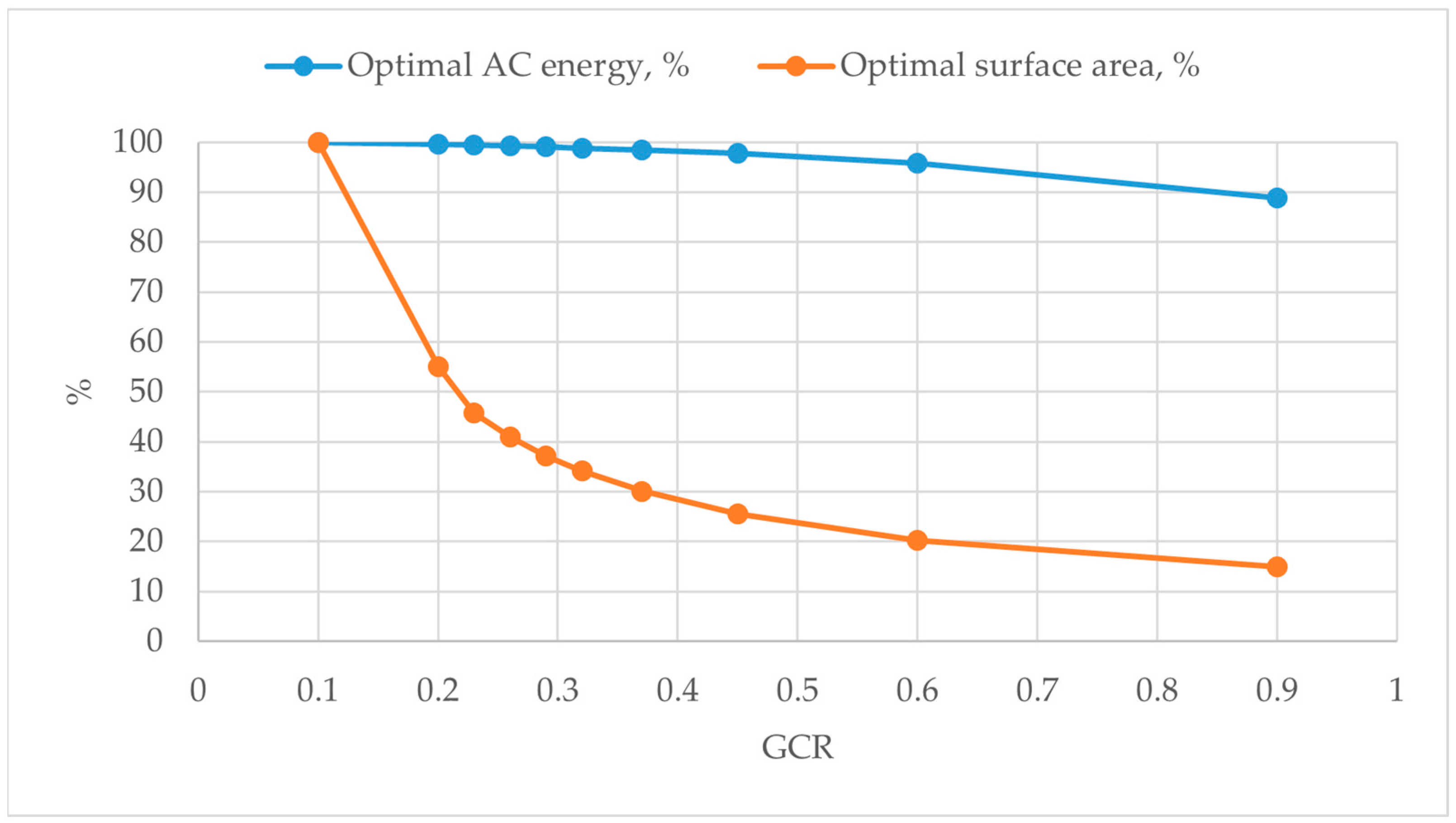
As expected, the PV system performs best with the lowest investigated GCR of 0.1, but the required installation surface area is 404.86 m
2, marked in bold as “Optimal surface area” of 100%. In this case, the system produced annual AC energy of 14,407.6 kWh/year, which is marked as “Optimal AC energy” of 100%,
Table 2. The default GCR in SAM is 0.3. The closest GCR value investigated is 0.29, and in this case, the system produced only 1% less energy, but requires a reduced installation area of 150.5 m
2, which is 37.2% of that for GCR = 0.1. What GCR is optimal depends on the case. Based on experience and the analysis of the data, the optimal GCR is somewhere in the range 0.3–0.6, where both curves are comparatively not too steep,
Figure 1. For this range, the annual AC energy produced is from 1 to 4% lower, which is acceptable, especially if the installation area is expensive. The final decision will depend on the available installation space and its price for a certain project.
For this research, for all projects consisting of 1 or 2 PV rows, the selected GCR is 0.1, although some projects have two rows oriented in different directions, and there are no additional similar structures at the front or the back that could cause shading. The GCR of 0.1 ensures that the SAM software will not subtract additional shading losses from the final result. For the PV system with 3 consecutive rows facing one direction, there are shading losses; therefore, a GCR = 0.29 is selected and used for the simulation. It ensures a performance close to the optimal system energy production, which is compared to that of the other systems, while the required installation surface area is comparatively low.
5. Experimental PV System Configurations
Two and three-string PV system configurations are created with the same 30 PV panels. This allows conclusions to be drawn from the perspective of the inverter’s operating efficiency according to the number of strings and their corresponding voltages, as well as separate comparisons of two and three-string systems with different azimuths. Preliminary analysis led to the conclusion that the PV system performance is comparatively tolerant to a non-optimal value for the azimuth if the tilt is optimal for the case. The conclusion is that the investigation of azimuth steps in 30° will lead to sufficiently accurate results, and these steps represent the major world directions. The optimal tilt for a given azimuth is presented in
Table 1.
With the same components, the following PV system configurations are created, as projects in SAM (Coding: Number of rows-Number of strings-Number of PV panels per string-Azimuths of the strings-GCR):
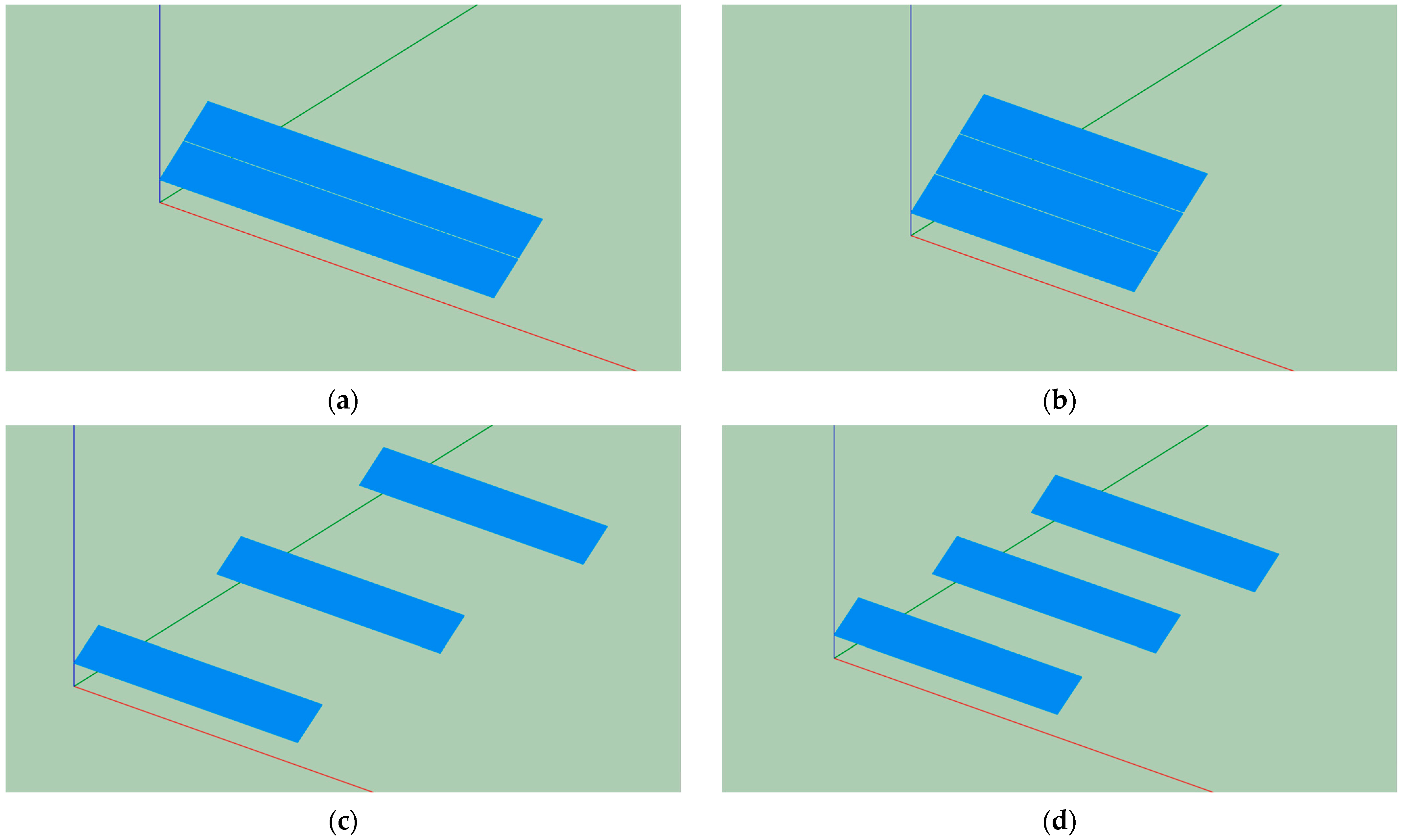
1-2-15-S—the PV panels are arranged in 1 row, but in 2 MPPT strings with 15 PV panels each, and with South (180°) azimuth,
Figure 2a.
1-3-10-S—the PV panels are arranged in 1 row, but in 3 MPPT strings with 10 PV panels each, and with South azimuth,
Figure 2b.
3-3-10-S-0.2—the PV panels are arranged in 3 rows, in 3 MPPT strings with 10 PV panels each, with South azimuth and GCR = 0.2,
Figure 2c. In certain cases, the installation surface area is not a problem, it is available, or cheap, and the low investment return ratios of the PV system for certain required power can be improved with higher row spacing, lower interrow shading, and better system performance. From this point of view, this case has been included in the comparison.
3-3-10-S-0.29—the PV panels are arranged in 3 rows, in 3 MPPT strings with 10 PV panels each, with South azimuth and GCR = 0.29,
Figure 2d.
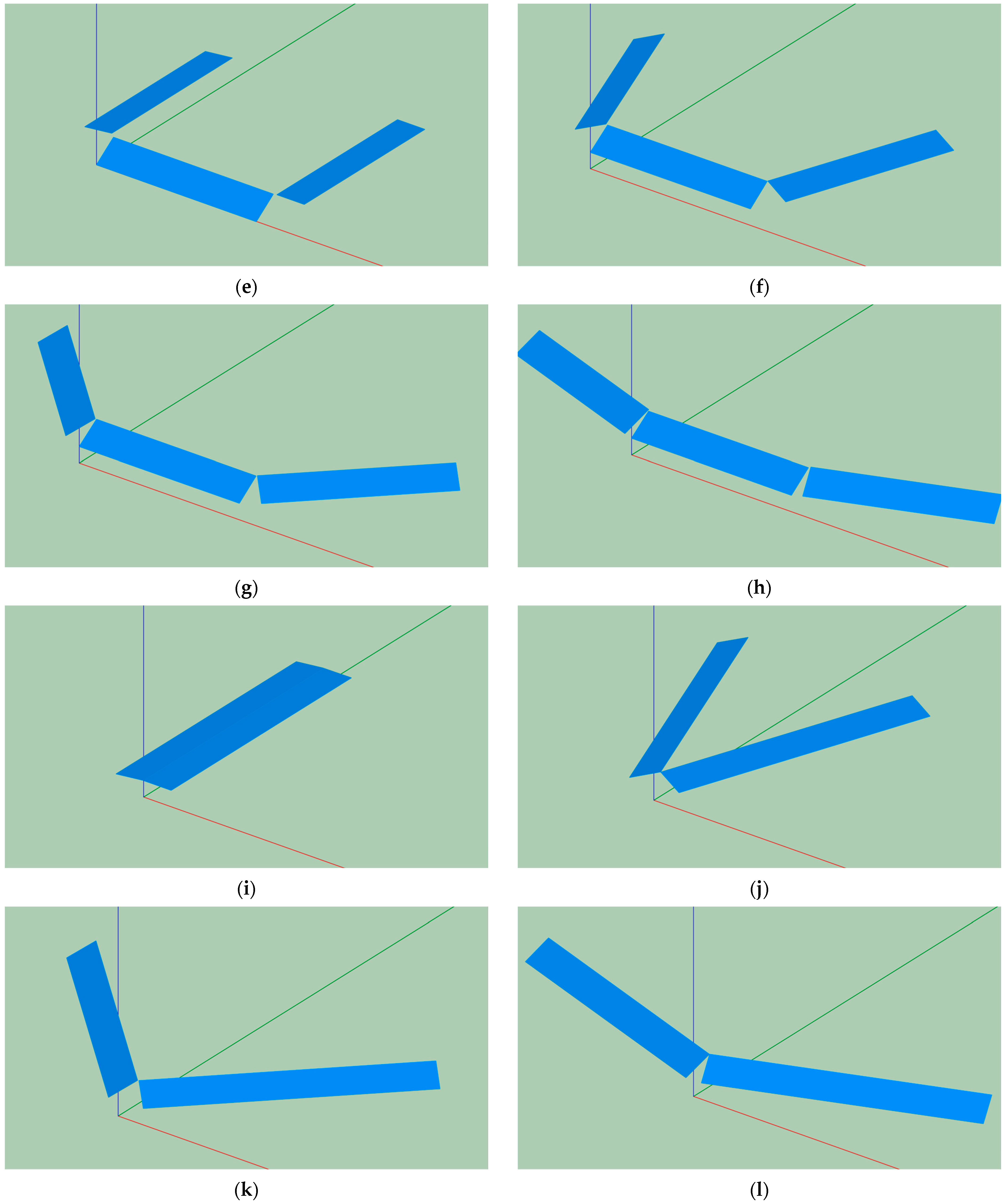
3-3-10-E/S/W—the PV panels are arranged in 3 rows, in 3 MPPT strings with 10 PV panels each, the different strings are with different azimuths East (90°), South (180°), and West (270°),
Figure 2e.
3-3-10-ESE/S/WSW—the PV panels are arranged in 3 rows, in 3 MPPT strings with 10 PV panels each, the different strings are with different azimuths East-South-East (110°), South (180°), and West-South-West (250°),
Figure 2f.
3-3-10-SE/S/SW—the PV panels are arranged in 3 rows, in 3 MPPT strings with 10 PV panels each, the different strings are with different azimuths South-East (135°), South (180°), and South-West (225°),
Figure 2g.
3-3-10-SES/S/SWS—the PV panels are arranged in 3 rows, in 3 MPPT strings with 10 PV panels each, the different strings are with different azimuths South-East-South (160°), South (180°), and South-West-South (200°),
Figure 2h.
2-2-15-E/W—the PV panels are arranged in 2 rows, in 2 MPPT strings with 15 PV panels each, the different strings are with different azimuths East (90°) and West (270°),
Figure 2i.
2-2-15-ESE/WSW—the PV panels are arranged in 2 rows, in 2 MPPT strings with 15 PV panels each, the different strings are with different azimuths East-South-East (110°) and West-South-West (250°),
Figure 2j.
2-2-15-SE/SW—the PV panels are arranged in 2 rows, in 2 MPPT strings with 15 PV panels each, the different strings are with different azimuths South-East (135°) and South-West (225°),
Figure 2k.
2-2-15-SES/SWS—the PV panels are arranged in 2 rows, in 2 MPPT strings with 15 PV panels each, the different strings are with different azimuths South-East-South (160°) and South-West-South (200°),
Figure 2l.
6. Results
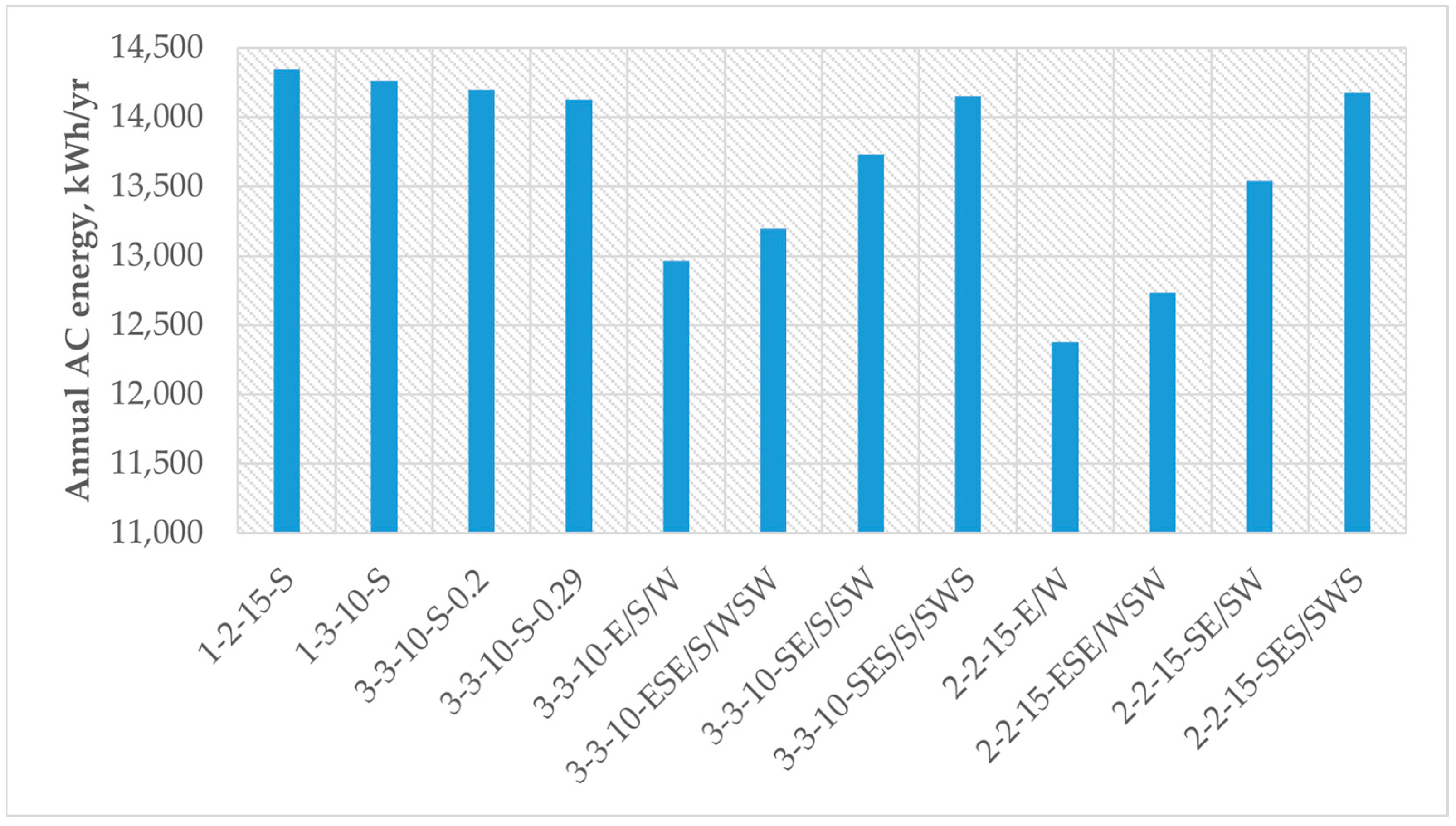
1-2-15-S has the highest annual energy production at 14,348 kWh/year, and the second-best, only 0.58% lower, is 1-3-10-S. For both systems, the designs are similar with PV panels oriented in the south direction, but the slight difference of 0.58% is due to the lower string DC voltages of 1-3-10-S, leading to lower power inverter efficiency,
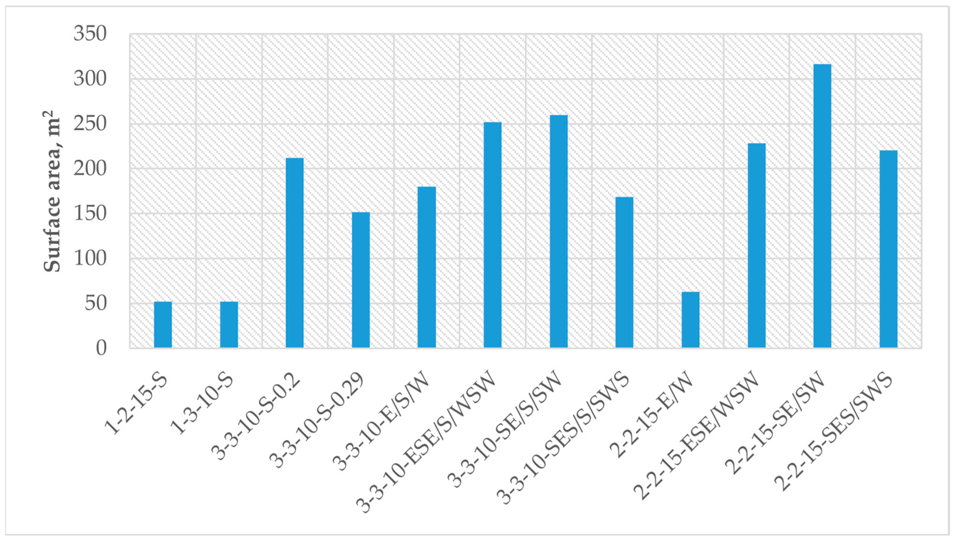
Figure 3. Their designs require the lowest horizontal installation space of 52.1 m
2 and are good for tilted rooftops, but their mounting structures are usually higher,
Figure 4.
Sorted by performance, 3-3-10-S-0.2, 2-2-15-SES/SWS, 3-3-10-SES/S/SWS, and 3-3-10-S-0.29 have lower energy generation than the maximum for 1-2-15-S, which is in the range of 1.04–1.54%. For 3-3-10-SE/S/SW, the difference is 4.48%, for 2-2-15-SE/SW—5.95%, and for 3-3-10-ESE/S/WSW it is 8.73%. For the rest, it is in the range 10.69–15.92%.
As expected, the PV systems with more PV panels oriented towards the South produce more energy, but they might not always be the best solution. With the rising number of PV capacities installed and without enough energy storage systems or other advanced control techniques, the energy prices tend to fall significantly, and even reach negative values at noon, a trend that has become normal for the Bulgarian free electricity market.
The 2-2-15-E/W is the second system requiring very low installation space of 62.75 m2, which is 1.2 times more than the minimum for 1-2-15-S, but it also produces the lowest amount of energy on an annual basis, which is 15.92% less than the maximum.
Sorted by installation space, the third best is 3-3-10-S-0.29, requiring 2.91 times higher installation area, followed by 3-3-10-SES/S/SWS at 3.24 times and 3-3-10-S-0.29 at 3.46. The rest of the designs need from 4 to 5 times more, the worst being 2-2-15-SE/SW, requiring 6.07 times higher installation area.
The 3-3-10-S-0.29 has comparatively low horizontal installation space requirements and offers high annual energy production. Besides allowing for a well-organized creation of complex multi-row PV plants, this design clearly offers a good balance between the required installation area and productivity. It is also one of the most common arrangements.
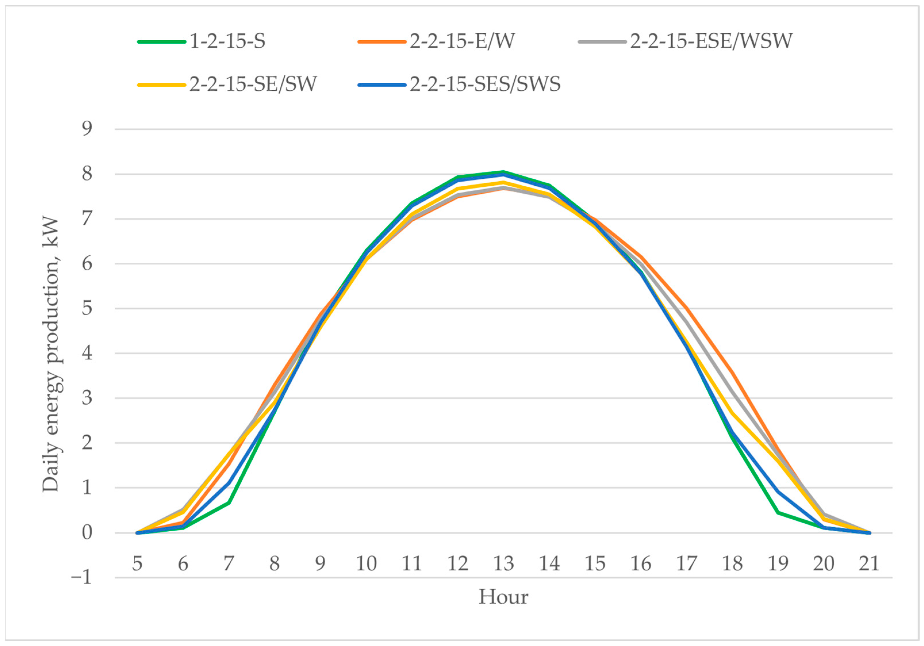
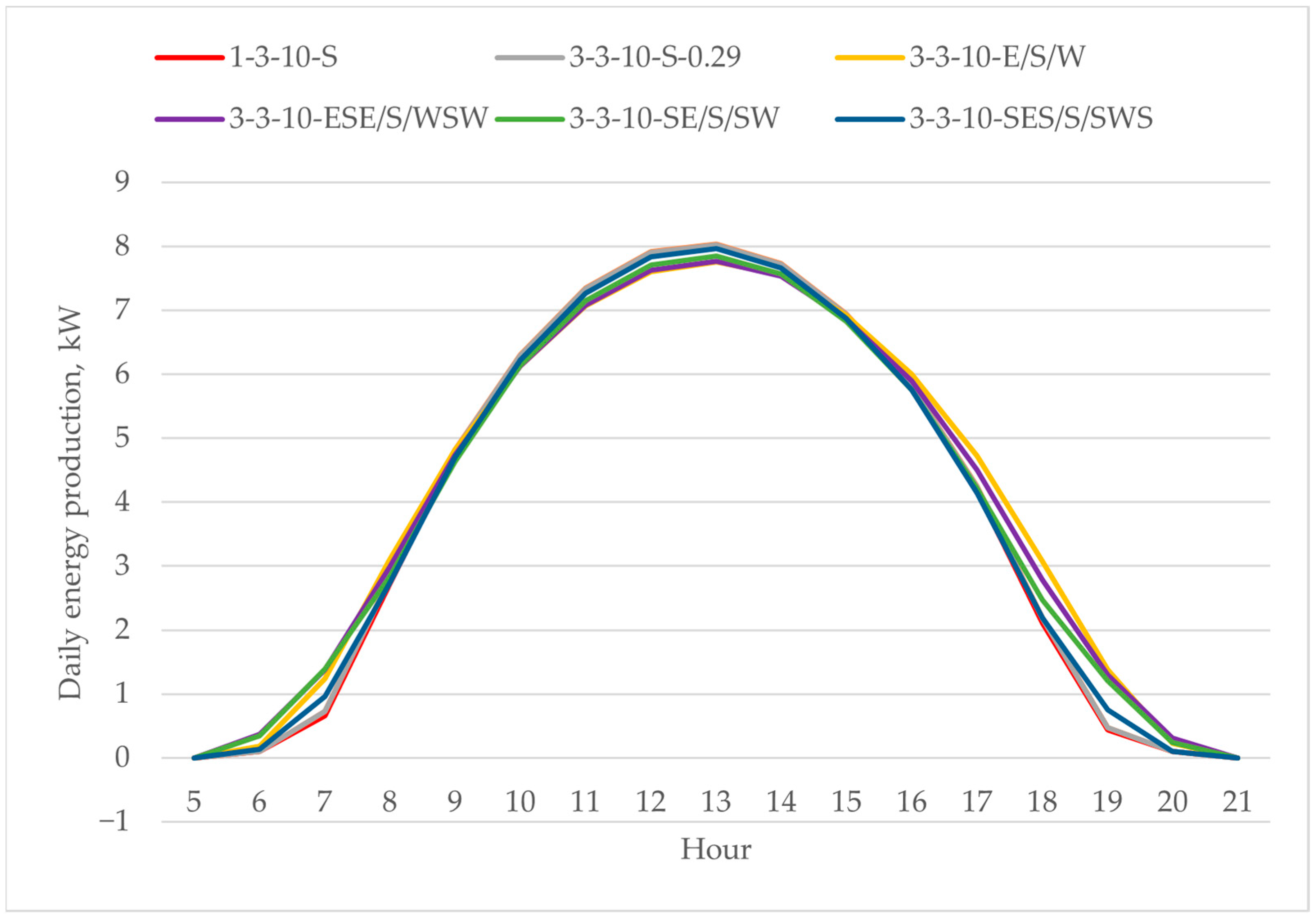
Which system returns more value depends on many factors. If the energy prices are regulated in the installation region and if there is one steady value for the whole day, then the system producing more energy and requiring lower installation space is the optimal choice. A good example is 1-2-15-S, but this design is good for small systems only, because it is not scalable for large plants. For large plants, the most common 3-3-10-S-0.29 is the best solution. If the energy prices depend on the free market, then without enough energy storage systems, they tend to fall sharply during the day, especially at noon, when PV systems produce the most energy. This is currently a common case at least in Bulgaria. In such situations, a PV system producing more energy in the morning and evening might be the best solution. Such systems have PV panels oriented more in the East and West directions, as shown in
Figure 5 and
Figure 6. If the difference in prices at noon compared to those in the morning and evening is large, then 2-2-15-E/W, with its low space requirements, might be the best solution. This design is scalable for large PV systems. Our conclusions from previous studies are that a more even daily energy generation and the earliest and latest energy production for East–West PV systems are achieved when configured with the optimal winter tilt. This might also require and a lower expensive energy storage capacity to conserve the excessive energy generated at noon for later use or sale at better prices in the evening [
37]. The 3-3-10-SES/S/SWS, but with better sizing of string DC voltages for higher inverter efficiency, offers a good balance between performance, space requirements, and scalability, and for large energy price deviations, it has the potential to return the same or even more value than the most common 3-3-10-S-0.29. The next best is 2-2-15-SES/SWS.
The conclusion is that different designs offer different benefits that can give an advantage in different situations; however, for small PV systems with limited space, the 1-2-15-S seems to be the best choice. Its main drawback is that, in certain cases, when installed on a horizontal surface, its supporting construction might be more expensive because of its larger size. Nevertheless, it could be perfect for tilted rooftops, no matter how many rows the panels are installed in, and if they are in portrait or landscape orientation, which depends on the form and size of the available installation spaces. The only problem with tilted rooftops is that their inclination may not be close to the optimal tilt. For large projects, designs such as 3-3-10-S-0.29 are more versatile and productive, but if there are large energy price deviations, other designs might return better value. Each case is different, and reliable simulation software can help to find the optimal solution for certain special circumstances.
7. Payback Period
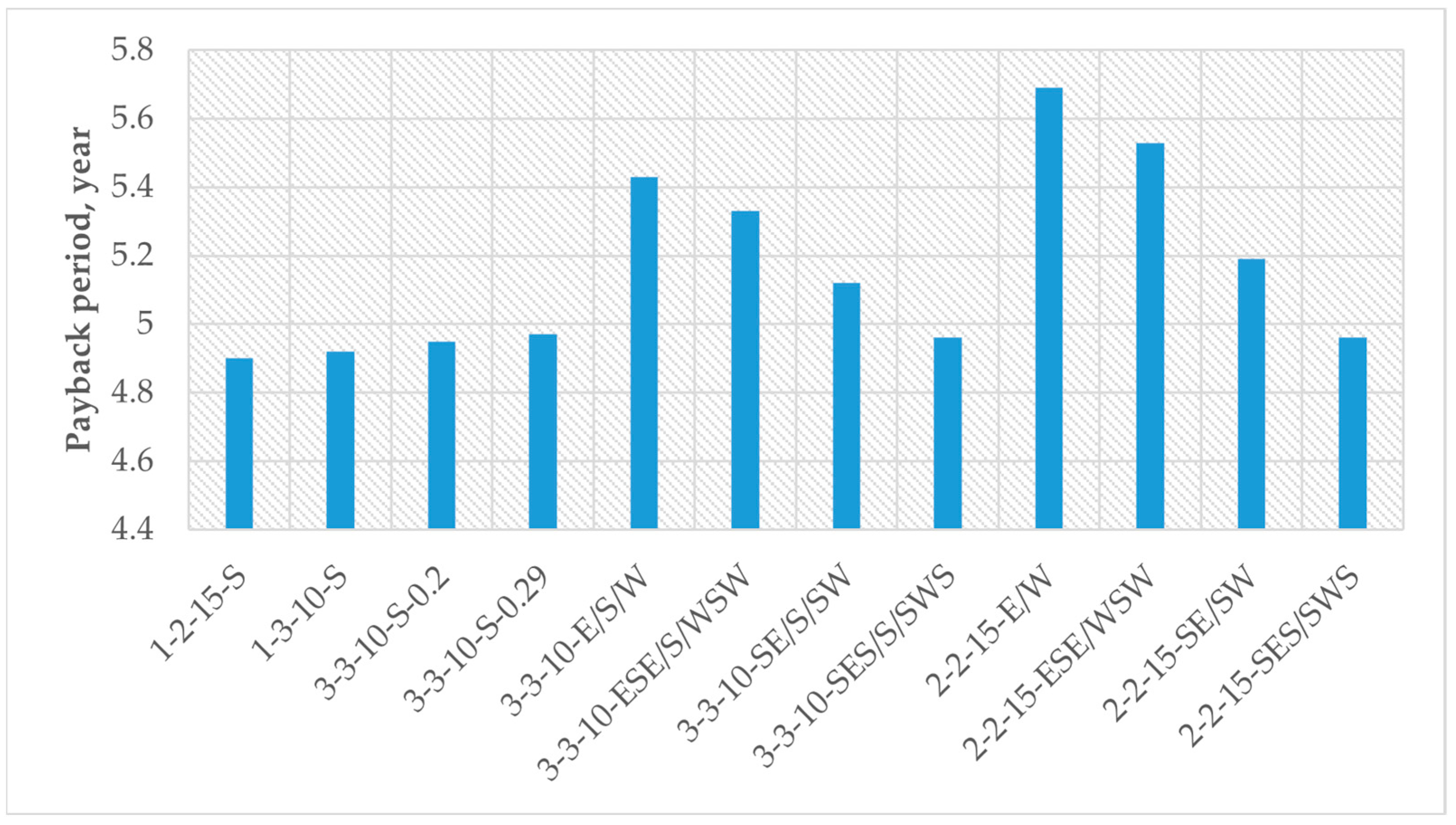
The simple payback period is calculated for the various grid-connected PV systems for the final regulated electricity price with a constant value of 0.15 Euro/kWh for private consumers in Bulgaria. The polycrystalline PV panels typically degrade at an average rate of 0.5% to 0.8% per year. The 0.8% annual degradation value is selected as a worst-case scenario, and the PV systems’ energy production is calculated for each separate year for a ten-year period. The energy production for each PV system for each separate year is multiplied by the constant electricity price for the Bulgarian private users of 0.15 Euro/kWh, and the result is the value returned per year. The PV system installation cost, including the price of the components and installation work, is 10,431 euros. No maintenance cost is added because the private consumers in Bulgaria usually do not pay such costs, and there probably will not be any during the system’s payback period. Based on the presented parameters, the simple payback period of the various PV systems is calculated and presented in
Figure 7.
The payback period for the various systems varies from 4.9 to 5.69 years. The shortest payback period is for 1-2-15-S, followed by 1-3-10-S, 3-3-10-S-0.2, 2-2-15-SES/SWS, 3-3-10-SES/S/SWS, 3-3-10-S-0.29. The difference between these designs is negligible because the values are in the range 4.9–4.97 years. The rest of the designs have a payback period over 5.12 years, with the worst being for 2-2-15-E/W.
The electricity prices constantly increase, and if this trend continues in the coming years, the actual payback period of the investment can could be shorter than calculated.
Furthermore, a complex economic analysis was not done, such metrics were not calculated, and the dependence pf the payback period on the constantly changing free market electricity prices for commercial users was not studied. This would be a very complex task for so many PV system configurations, as it would generate a large amount of new data, and is therefore beyond the scope of this work. This is left for future investigation. A similar analysis was done in the past for PV systems with South and East–West PV panel azimuths only. It concluded that the most energy-producing South azimuth may not be the optimal case when too much PV capacity is installed as a percentage of the total grid power, which leads to wider daily energy price spreads and close-to-zero energy prices at noon. When all factors are taken into consideration, the East–West Azimut PV system with an optimal winter tilt offers an even daily energy generation and the potential to outperform all other system configurations [
37].
8. Discussion
The designs that are not scalable for large multi-row systems are 3-3-10-E/S/W, 3-3-10-ESE/S/WSW, and 2-2-15-ESE/WSW. In order to avoid considerable shading, these designs require higher row spacing and for large systems will require a larger installation space.
The most common design for large systems is that with a South azimuth,
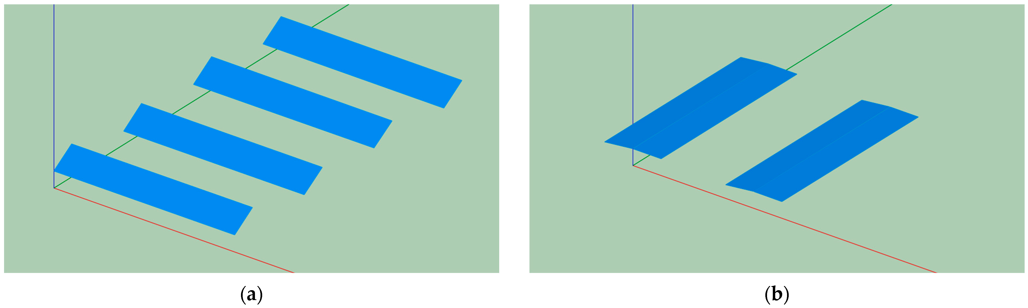
Figure 8a. Among the rest, the East–West azimuth has an inherent advantage,
Figure 8b. It allows more PV panels to be installed in the same installation area if minimal separating space is left between adjacent East and West PV panel rows. For larger PV systems with many PV rows, the required installation area for a certain peak power is from 50 to 60% lower for the East–West in comparison to that for the South azimuth design if the row spacing is the same. The difference depends on the GCR, PV panel sizes and tilts, how large the system is and other factors. In this investigation, the East–West example is 2-2-15-E/W, which produced 87.6% of the annual energy generated by the most common South design 3-3-10-S-0.29. If the difference in inverter efficiency of 0.58% is subtracted because of the different DC voltages of both systems, then the more accurate result is 87.1%. From functionality and return on investment perspectives, this difference in the energy production of both systems could be compensated for the East–West system, either by high daily energy price deviations or by a lack of sufficient installation space for the power needed or too expensive land. The East–West azimuth systems generate electricity the earliest in the morning and the latest in the evening, when energy prices could be more than 10 times higher than those at noon. This happens when the PV capacities have a comparatively high share un the energy mix, usually over 20%, and when there are not enough energy storage systems, which is a common case nowadays. In such cases, energy prices often fall to close to zero or even negative values at noon, while in the morning or evening, they might be hundreds of euros per MWh, which depends on the energy mix and the balance between supply and demand. The world is currently in an accelerated green transition, and in many European countries, there is a shortage of electricity at certain times of the day and too much at others, which creates anomalies in electricity prices.
The 3-3-10-SES/S/SWS, but with better sizing of string DC voltages for higher inverter efficiency, offers a good balance between performance, space requirements, and scalability; for large energy price deviations, it also has the potential to return the same or even more value than the most common 3-3-10-S-0.29.
The East and West azimuths and their combinations with the South possess unique qualities and allow many more rooftop areas in urban environments to be used for the installation of PV systems. A study concluded that only around 20% of the total rooftop area in València is classified as fully suitable for solar PV panel installation [
38], but if we accept that the orientation of the rooftops is more often in four directions and the combinations of East, South and West are suitable, the conclusion from a more detailed analysis should be that about 50 to 75% of them should be good for such installations. At least this could be the conclusion for Bulgaria because the majority of houses here have hip roofs; gable roofs are less common, and flat roofs are usually common for tall buildings, which constitute a relatively small percentage of the total. In Bulgaria, the inclination of hip and gable roofs varies, often between 20° and 35°, which is close to the optimal tilt values for different azimuths for Bulgaria, presented in
Table 1. The PV panels on flat rooftops can always be arranged in several different directions, if needed. There is no common average surface area for roofs in Bulgaria, but depending on the house, it often varies between 80 and 180 m
2, which is enough to cover the majority of a household’s energy needs.
9. Conclusions
The different PV panel configurations offer various advantages and disadvantages in different situations. The best configuration depends on the requirements of each specific case and on many factors. These include regional energy prices, which could be comparatively constant or changing and defined by the free market. In both cases, if the goal is the highest energy yield, the South azimuth might be best, but if there are requirements for a more even daily energy generation, or generation earlier in the morning and later in the evening, then one of the presented configurations with a certain number of strings oriented more in the East or West directions might offer better performance for the given consumer profile. The PV system performance for non-optimal azimuths can be improved by tilt optimization.
An expensive or limited installation area requires a PV system configuration optimized for spatial efficiency, but still offering the necessary performance. Reliable simulation software, such as SAM and PVsyst, is a valuable and indispensable tool for the timely optimization of PV systems for many specific cases.
1-2-15-S has the highest annual energy production at 14,348 kWh/year, and the second-best, only 0.58% lower, is 1-3-10-S. Sorted by performance, 3-3-10-S-0.2, 2-2-15-SES/SWS, 3-3-10-SES/S/SWS, and 3-3-10-S-0.29 have lower energy generation than the maximum for 1-2-15-S, which is in the range of 1.04–1.54%. For 3-3-10-SE/S/SW, the difference is 4.48%, for 2-2-15-SE/SW—5.95%, and for 3-3-10-ESE/S/WSW it is 8.73%. For the remaining configurations, the difference is in the range 10.69–15.92%.
1-2-15-S is also the system with the lowest horizontal installation space of 52.1 m2. The 2-2-15-E/W is the second system requiring very low installation space of 62.75 m2, which is 1.2 times larger than the minimum, but it also produces the lowest amount of energy on an annual basis, which is 15.92% less than the maximum. Sorted by installation space, the third best is 3-3-10-S-0.29, requiring 2.91 times more installation area, followed by 3-3-10-SES/S/SWS at 3.24 times and 3-3-10-S-0.29 at 3.46. The rest of the designs need between 4 and 5 times more space, the worst being 2-2-15-SE/SW, requiring 6.07 times higher installation area.
The general guidelines are that the single-row South PV systems (1-2-15-S) perform best and require the least horizontal installation space, but are generally suitable for comparatively small PV plants and for installations on tilted rooftops. Their supporting structures could be created on flat rooftops, but for a certain power, the structure is heavier and higher, and must be strengthened against strong winds because it is practically one large sail. When installed on tilted rooftops, depending on the case, PV panels arranged in different strings could be installed on East, South-East, South, South-West, and West slopes for generating energy early in the morning and late in the day, when energy prices are usually higher.
The multi-row South PV systems (3-3-10-S-0.29) are the most widely used and versatile, making them good for both small and large projects. They offer comparatively high performance and an average installation space requirement. Their GCR could be selected depending on the requirements of the project, but values between 0.3 and 0.6 seem to be optimal for most cases. A higher GCR means lower required installation area but also lower energy generation. They are suitable for installation on flat surfaces or rooftops.
All South azimuth PV systems are generally good when one of the requirements is high performance, although they generate too much energy at noon. Consequently, they are generally suitable for energy prices with comparatively low daily fluctuations, but this also depends on the case-specific energy consumption profiles and how the potentially excessive noon energy is treated.
The rest of the designs offer more even daily energy generation patterns, which might also require a lower, less expensive energy storage capacity to conserve the excessive energy generated at noon for later use or sale at better prices in the evening. The best in this regard is the East–West PV system, especially with an optimal winter tilt, which is based on previous works [
37].
For large projects, the East–West PV system requires 50–60% lower installation surface area than a multi-row South system for the same peak power, but depending on the selected tilt, it might generate from 15 to 30% less energy per year. It is suitable for flat surfaces and for regions with high daily energy price deviations. The currently common high morning and evening energy prices, and very low noon ones, could considerably improve its rate of value return in comparison to the other investigated designs [
37].
Due to the required higher row spacing, the 3-3-10-E/S/W, 3-3-10-ESE/S/WSW, and 2-2-15-ESE/WSW designs are not suitable for large PV systems, but might offer benefits for small ones, especially for high daily energy price deviations and when there are requirements for a balance between more even daily energy generation and performance. The problem with these configurations is that they are not suitable for large multi-row systems, because in order to avoid inter-row shading, high row spacing must be selected, and this is not space-efficient for installation. They are suitable for one-row systems installed on flat surfaces. They can be applied if the PV panels are installed as eaves at the ends of flat roofs or above windows.
The 2-2-15-SE/SW requires the highest installation area without any obvious advantages.
The payback period for the various systems, calculated with the final regulated electricity price with a constant value of 0.15 Euro/kWh for private consumers in Bulgaria, varies from 4.9 to 5.69 years. The shortest payback period is for 1-2-15-S, followed by 1-3-10-S, 3-3-10-S-0.2, 2-2-15-SES/SWS, 3-3-10-SES/S/SWS, and 3-3-10-S-0.29. The difference between these designs is negligible because the values are in the range of 4.9–4.97 years. The rest of the designs have a payback period over 5.12 years, with the worst being for 2-2-15-E/W. The dependence of the payback periods on the constantly changing free market electricity prices is complex to calculate and is therefore beyond the scope of this work.
Another limitation of this work is that the necessary energy storage capacity needed for the generated excess electricity at certain times of the day or for sale at better prices has not been addressed. This is a complex study and is also beyond the scope of this work.
This work is part of a large-scale study on optimizing peak power, design, storage capacity, lifetime, and return on investment in photovoltaic systems for specific energy profiles of consumers. Its main conclusion is that for every case, there is a right PV system configuration that performs best.