Cross-Coupled Conditional Funnel Control: A Model-Free Approach for Load-Following Operation of Pressurized Heavy Water Reactor

Abstract

This study presents the design of a model-free control scheme for the load-following operation of a Pressurized Heavy Water Reactor (PHWR), which is a 70th-order Multi-Input Multi-Output, strongly coupled and open-loop unstable energy-generating system. To design a model-free controller for a PHWR, we propose a novel cross-coupled conditional error surface and a modified funnel algorithm-based funnel control scheme. The proposed control scheme reduces the effects of inter-zonal coupling and improves the steady-state accuracy without degrading the transient performance. The proposed control scheme is of low complexity and does not require system dynamics for controller design. A closed-loop stability analysis is carried out to ensure the boundedness of the closed-loop system trajectories. Furthermore, the proposed control scheme is evaluated by simulating different scenarios, which demonstrate its effectiveness.

1. Introduction

The electrical energy generated by nuclear power plants is economical and has a low carbon footprint in contrast to fossil fuel-based power plants. However, in comparison with fossil fuel-based power plants, a major drawback associated with nuclear power plants is the complexity of their systems, especially the nuclear reactors in which heat energy is produced through a fission chain reaction. The heat energy is regulated by controlling the chain reaction taking place in the reactor core. This chain reaction is controlled through reactivity-controlled devices. There are different types of nuclear reactors. One such reactor type is the large Pressurized Heavy Water Reactor (PHWR), which is a 70th-order complex, coupled, and open-loop unstable dynamical system with 14 inputs and 14 outputs [1].

Due to advantages such as cheap energy production and a negligible carbon footprint, the share of electrical power generated by nuclear power plants in the electrical grid is increasing. With the growing number of nuclear power plants in the electrical grid, the load-following operation for nuclear reactors is a natural selection over the base-load operation [2]. Thus, the design of a controller that is capable of controlling reactor power to efficiently follow load demand is essential. In addition to good load-following and robust capabilities, the controller should be able to effectively balance flux tilting and the rejection of disturbances.

Several control schemes have been reported in the literature for the load-following operation of heavy water nuclear reactors. For instance, in [3], spatial control of a large PHWR is proposed using a fast-output sampling technique. The authors of [4] propose a decentralized scheme using periodic-output feedback for spatial control of a large PHWR. A multi-rate output feedback-based sliding mode control (SMC) scheme for a large PHWR is proposed in [5]. A decentralized control scheme based on the LQR technique is proposed in [6,7] for a large PHWR. An output feedback SMC scheme is presented in [8,9] for a PHWR. An SMC technique is also proposed in [10] for spatial stabilization of an Advanced Heavy Water Reactor (AHWR). A robust fractional-order proportional–integral control scheme is suggested in [11] for a PHWR. An SMC scheme based on a fuzzy logic approach is developed in [12] for the spatial control of an AHWR, whereas integral SMC schemes based on an LQR technique are proposed in [13] and [14] for the spatial control of a large PHWR and an AHWR, respectively. Recently, a fractional-order proportional–integral–derivative control scheme using an enhanced crow search algorithm was suggested in [15] for a PHWR. Notice that all the foregoing control schemes are linear; that is, their design is based on the linearized process model, which is obtained by linearizing the nonlinear process dynamics around an operating point. In comparison with nonlinear control methods, there are two drawbacks associated with linearized control schemes: (1) the linear system dynamics are not rich enough and (2) linear control schemes guarantee only local behavior [16,17]. Thus, the performance of linear control schemes cannot be guaranteed outside a narrow region around the operating point.

To attain performance specifications such as good load following and robust capabilities, nonlinear and intelligent control techniques have been proposed for the control of nuclear reactors. In the domain of nonlinear controllers, the SMC scheme has been most extensively studied for the control of nuclear reactors. For instance, a variety of SMC schemes are proposed in [2,17,18,19,20] for the control of a pressurized water reactor (PWR). The SMC schemes used in these works comprise an equivalent control part and a switching control part; the design of the equivalent control part utilizes the system dynamics and, hence, dynamical knowledge of the process model is required to design these SMC schemes.

In the area of intelligent control schemes, the Fuzzy Logic Control (FLC) approach has been widely considered for the control of nuclear reactors. For instance, in [21,22], an FLC scheme is suggested for the control of a PHWR, whereas in [23], an FLC scheme is proposed for the control of VVER-1200 nuclear reactors. However, the FLC scheme requires a good understanding of the process model or at least the experience of a system operator for designing its rule base. Furthermore, the FLC scheme consists of Fuzzification, rule base, Inference Mechanism and Defuzzification units; thus, it requires considerably large computational resources in comparison with controllers, such as PID, LQR and H_∞ techniques.

Designing the abovementioned control schemes requires complete knowledge of the process model, and their performance depends on the accuracy of the process model or the understanding of the process dynamics. Since PHWR is a coupled dynamical process, the change in power in one zone disturbs the power in other zones, and, therefore, the effects of coupling between the zones should be minimized to achieve smooth regulation of the reactor power to the demanded power. To reduce the effects of coupling, centralized and decentralized algorithms, such as centralized PID and decentralized PID, have been widely studied in the literature [24]. However, the design of centralized and decentralized algorithms is complex, and they require linearized system dynamics. Furthermore, the performance of decentralized algorithms is not satisfactory for large systems.

From the above discussions, the focus of this study is to present a novel study on the design of a low-complexity and model-free controller for robust tracking of power demand for a large PHWR process. To accomplish this goal, we consider the funnel control, which was proposed in [25], for relative degree-one systems. The astonishing feature of the funnel control is its design simplicity while relaxing the requirements of the knowledge of process dynamics a priori. However, the implementation of the funnel control suffers from the drawback that the error surface may escape the funnel boundary, leading the controller to instability if the reference signal is not sufficiently smooth enough. This causes difficulty in the load-following operation of the PHWR using the funnel control approach. To solve this problem, a modified funnel function is presented in this study, which is the modified version of the algorithm proposed in [26]. Furthermore, to improve the steady-state error accuracy, usually, an integral action is used; however, integral control degrades the transient response of the closed-loop system [27]. The concept of conditional funnel control is proposed in [28], which improves the steady-state accuracy of the funnel control scheme; however, the proposed technique requires partial dynamical function of the system and, thus, it does not offer a model-free solution. Furthermore, the controllers proposed in [26,28] are designed for SISO systems. Thus, to improve the steady-state error accuracy without degrading the transient performance, reducing the inter-zonal coupling disturbances and providing a model-free control solution, we propose Cross-Coupled Conditional Funnel Control (CCC-FC) for the control of PHWR. To the best of the authors’ knowledge, the CCC-FC is proposed for the first time. Hence, following are the main contributions of this study:

• In comparison with the previously proposed linear control schemes [3,4,5,6,7,8,9,11,13,15], in this study, a nonlinear control scheme is proposed for a large PHWR, which efficiently tracks demanded power while effectively rejecting input disturbances.
• The cross-coupled terms are introduced in the funnel control architecture, which reduce the effects of inter-zonal coupling and, thus, relax the use of complex linear techniques such as detuning and decoupling algorithms.
• In comparison with the control schemes in [1,2,3,4,5,6,7,8,9,10,11,13,14,15,17,18,19,20,21,22,23], the design procedure of the proposed scheme is of low complexity. Furthermore, the controllers designed in [13,14,29] require full states (that is, all the states of the process) as feedback, whereas the proposed controller only requires the output states and their derivatives as feedback.
• In comparison with the control schemes in [1,2,17,18,19], the requirement for the dynamical functions of the PHWR model in designing the controller is completely relaxed; thus, in this context, the proposed control scheme offers a model-free solution.
• In comparison with the fuzzy control schemes in [21,22,23], the knowledge of the experienced PHWR operator or knowledge of the PHWR process expert is not required in designing the proposed control scheme.

Although the design of the proposed control approach does not require any dynamical function of the PHWR model, suitable selection of its parameters is required to achieve the desired performance. Therefore, a detailed guideline for parameter selection is provided in Section 5. Nevertheless, the complete design procedure of the proposed control approach is less complex than that given in [1,2,3,4,5,6,7,8,9,11,13,15,17,18,19,20,21,22,23].

The scope of this study is to propose a low-complexity control scheme for the PHWR process by utilizing the funnel control approach, which (1) ensures the steady-state accuracy without degrading the transient performance, (2) reduces the inter-zonal coupling disturbances, (3) tracks the reference signal efficiently while rejecting the input disturbances, and (4) does not require any dynamical function of the PHWR model in its design. The rest of this paper is arranged as follows: an introduction to the PHWR process along with the conversion of PHWR dynamics into error form is given in Section 2; an introduction to funnel control is given in Section 3; the design of Cross-Coupled Conditional Funnel Control (CCC-FC) is presented in Section 4; simulation results are discussed in Section 5; and, finally, this study is concluded in Section 6.

Nomenclature: In this study, the following notations are used: $\mathbb{R}$ represents a set of real numbers, whereas ${\mathbb{R}}_{+}$ and ${\mathbb{R}}_{\ge 0}$, respectively, represent a set of positive real numbers and real numbers greater than zero; $W^{1,\infty }\left({\mathbb{R}}_{\ge 0},{\mathbb{R}}_{+}\right)$ denotes a class of bounded functions having bounded derivatives; $\inf \left(.\right)$ and $\sup \left(.\right)$, respectively, represent the infimum and supremum of the argument; $‖⦁‖$ and $\left|⦁\right|$, respectively, represent norm and the absolute value of “$⦁$”; $\mathrm{s}\mathrm{g}\mathrm{n}\left(.\right)$ and $\mathrm{s}\mathrm{a}\mathrm{t}\left(.\right)$ are, respectively, the standard signum and saturation functions; and ${\lambda }_{\mathrm{m}\mathrm{i}\mathrm{n}}\left(.\right)$ denotes the minimum eigenvalue of the argument.

2. Pressurized Heavy Water Reactor (PHWR)

A Pressurized Heavy Water Reactor (PHWR) is an open-loop, unstable, coupled dynamical system in which heavy water is used as a moderator as well as a coolant, whereas natural Uranium is used as a fuel source. The PHWR considered in this work has a large core that produces around 1800 MW of thermal energy. Due to its large dimensions, the reactor core is divided into 14 zones for managing spatial power. Thus, each zone is coupled to other zones through coupling coefficients, and the power in each zone is controlled through Liquid-Zone Compartment (LZC). Thus, the PHWR studied in this work is a complex 70th-order energy-generating system consisting of 14 inputs and 14 outputs [5]. The modeling of a PHWR along with its validation against benchmark experimental data is given in [30]. The dynamics of the PHWR in normal form is described as follows [1,5,8,9]:

$${\dot{\eta }}_{Ci}=h_{Ci}({\eta }_{Ci},z_{i,1})=-{\lambda }_c{\eta }_{Ci}+{\displaystyle \frac{\beta }{l}}{z}_{i,1}$$

(1)

$${\dot{\eta }}_{Ii}=h_{Ii}({\eta }_{Ii},z_{i,1})={\gamma }_I{\Sigma }_f{z}_{i,1}-{\lambda }_I{\eta }_{Ii}$$

(2)

$${\dot{\eta }}_{Xi}=h_{Xi}({\eta }_{Xi},{\eta }_{Ii},z_{i,1})={\gamma }_X{\Sigma }_f{z}_{i,1}+{\lambda }_I{\eta }_{Ii}-\left[{\lambda }_X+{\overline{\sigma }}_{Xi}{z}_{i,1}\right]{\eta }_{Xi}$$

(3)

$${\dot{z}}_{i,1}=z_{i,2}$$

(4)

$${\dot{z}}_{i,2}=f_i({\eta }_{Ci},{\eta }_{Xi},{\eta }_{Ii},z_{i,1},z_{i,2})+g_i\left(z_{i,1}\right)q_i$$

(5)

where f_i(.) and g_i(z_i,1) are, respectively, defined as follows:

$$f_i\left(.\right)=f_{i,1}({\eta }_{Ci},{\eta }_{Xi},{\eta }_{Ii},z_{i,1},z_{i,2})+f_{i,2}(z_{i,1},z_{i,2})$$

(6a)

$$g_i\left(z_{i,1}\right)={\displaystyle \frac{K_i{m}_i}{l}}{z}_{i,1}$$

(6b)

where f_i,1(.) and f_i,2(.) are, respectively, given as follows:

$$f_{i,1}\left(.\right)=-{\displaystyle \frac{{\sigma }_{Xi}}{l{\mathrm{\Sigma }}_{\mathrm{a}}}}{h}_{Xi}{z}_{i,1}+\left(z_{i,2}-{\lambda }_c{\eta }_{Ci}\right){\displaystyle \frac{z_{i,2}}{z_{i,1}}}+{\lambda }_c{h}_{Ci}$$

(6c)

$$f_{i,2}\left(.\right)={\displaystyle \frac{1}{l}}{\displaystyle {\sum }_{j=1}^N}{\alpha }_{j,i}\left(z_{j,2}-z_{j,1}{\displaystyle \frac{z_{i,2}}{z_{i,1}}}\right)$$

(6d)

where $i=1 to N$ and $N=14$; $z_{i,1}\left(t\right)$, ${\eta }_{Ci}\left(t\right)$, ${\eta }_{Xi}\left(t\right)$ and ${\eta }_{Ii}\left(t\right)$ are, respectively, the thermal power (in MW), normalized delayed neutron concentration (in MW), normalized Xenon concentration (in MW·cm⁻¹·s) and normalized Iodine concentration (in MW·cm⁻¹·s) of the i-th zone; $\alpha$ is the coupling coefficient (dimensionless); $\beta$ is the fractional yield (dimensionless); ${\lambda }_c$, ${\lambda }_X$ and ${\lambda }_I$ are, respectively, the delayed neutron, Xenon and Iodine decay constants (in s⁻¹); ${\overline{\sigma }}_{Xi}$ is the normalized microscopic thermal neutron absorption cross-section of Xenon (in MW⁻¹·s⁻¹) for the i-th zone; ${\gamma }_I$ and ${\gamma }_X$ are, respectively, the Iodine and Xenon yields (dimensionless); $K_i<0$ and $m_i>0$ are LZC constants; $q_i$ is the input to the i-th zone; and $l$ is the prompt neutron lifetime (in s). The global (total) power of the reactor can be computed as follows:

$$z_g={\displaystyle {\sum }_{i=1}^N}{z}_{i,1}$$

(6e)

Remark 1.

η_Yi and z_i are, respectively, known as the internal and external dynamics of the considered PHWR system.

Property 1.

The reactor zonal powers cannot be negative, that is, z_i,1 ≥ 0.

Property 2.

The relative degree of the PHWR is 2.

The design of a stable tracking controller is possible if the internal dynamics of the PHWR remain stable over the entire region of interest [31,32]. Thus, the following Lemma ensures that the zero dynamics of the PHWR remain stable.

Lemma 1.

The zero dynamics of the system described in Equations (1)–(5) remain stable if the following conditions hold:

$${\lambda }_c>0$$

(7a)

$${\lambda }_I>0$$

(7b)

$${\lambda }_X+{\overline{\sigma }}_{Xi}{r}_i>0$$

(7c)

Proof. 

Please refer to the proof of Lemma 1 in [1]. □

Transformation into Error Coordinates

For the design of a controller and stability analysis of the closed-loop system, the external dynamics need to be transformed into the error dynamics structure. Therefore, let

$$e_{i,1}=z_{i,1}-r_i$$

(8a)

$$e_{i,2}=z_{i,2}-{\dot{r}}_i$$

(8b)

where $r_i$ is the reference signal of the i-th zonal power. Now, the dynamics given in Equations (1)–(5) can be represented in the structure of error coordinates as follows:

$${\dot{\eta }}_{Ci}=h_{Ci}({\eta }_{Ci},e_{i,1}+r_i)=-{\lambda }_c{\eta }_{Ci}+{\displaystyle \frac{\beta }{l}}\left(e_{i,1}+r_i\right)$$

(9)

$${\dot{\eta }}_{Ii}=h_{Ii}({\eta }_{Ii},e_{i,1}+r_i)={\gamma }_I{\Sigma }_f\left(e_{i,1}+r_i\right)-{\lambda }_I{\eta }_{Ii}$$

(10)

$${\dot{\eta }}_{Xi}=h_{Xi}({\eta }_{Xi},{\eta }_{Ii},e_{i,1}+r_i)={\gamma }_X{\Sigma }_f\left(e_{i,1}+r_i\right)+{\lambda }_I{\eta }_{Ii}-\left[{\lambda }_X+{\overline{\sigma }}_{Xi}\left(e_{i,1}+r_i\right)\right]{\eta }_{Xi}$$

(11)

$${\dot{e}}_{i,1}=e_{i,2}$$

(12)

$${\dot{e}}_{i,2}=f_i\left({\eta }_{Ci},{\eta }_{Xi},{\eta }_{Ii},z_{i,1},z_{i,2}\right)-{\ddot{r}}_i+g_i\left(z_{i,1}\right)q_i$$

(13)

Assumption 1.

The reference signal r_i and all its derivatives are bounded.

3. Introduction to Funnel Control

The theory behind funnel control is to increase the gain when the error approaches the prescribed boundary known as the funnel boundary. Consider a MIMO system defined as ${\dot{x}}_i=f_i\left(x\right)+g_i\left(x\right)u_i$, where $g_i\left(x\right)<0$ and i = 1 to M, with M representing the total number of subsystems, each having relative degree one. Before introducing the funnel control, consider the following definitions [25,33,34]:

$${\varphi }_i≔\left\{{\phi }_i ϵ W^{1,\infty }\left({\mathbb{R}}_{\ge 0},{\mathbb{R}}_{+}\right) | \forall \overline{\tau }\ge 0: {\phi }_i\left(\overline{\tau }\right)>0 \mathrm{a}\mathrm{n}\mathrm{d} \underset{\overline{\tau }\to \infty }{\lim }\inf {\phi }_i\left(\overline{\tau }\right)>0\right\}$$

(14)

$${\overline{\mathcal{F}}}_{{\phi }_i}≔\left\{\left(t,e_i\right)\in {\mathbb{R}}_{\ge 0}\times \mathbb{R}:{\phi }_i\left(t\right)\left|e_i\right|<1\right\}$$

(15)

where $e_i\left(t\right)=y_i-r_i$, with $y_i=x_i$ being the output and $r_i$ being the reference signal. The funnel control is defined as follows:

$$u_i\left(t\right)={\overline{k}}_i\left(t\right)e_i\left(t\right)$$

(16)

The gain ${\overline{k}}_i\left(t\right)$ is defined as follows:

$${\overline{k}}_i\left(t\right)={\displaystyle \frac{1}{{\psi }_i\left(t\right)-\left|e_i\left(t\right)\right|}}$$

(17)

where ${\psi }_i\left(t\right)$ is the funnel boundary. In this study, we consider the following funnel function, which is extensively reported in the literature [33,34,35]:

$${\phi }_i\left(t\right)={\psi }_i^{-1}\left(t\right)={\left[\left({\psi }_{i,0}-{\psi }_{i,\infty }\right)\exp \left(-{\varsigma }_{i}t\right)+{\psi }_{i,\infty }\right]}^{-1}$$

(18)

where ${\psi }_{i,0}>0$, ${\psi }_{i,\mathrm{\infty }}>0$ and ${\varsigma }_i>0$ are constants.

Remark 2.

If  $e_i\left(0\right)<{\psi }_i\left(0\right)$, the funnel control guarantees a change in the error trajectory from  $e_i\left(0\right)$  to a narrow strip  $\left[-{\psi }_{i,\infty },{\psi }_{i,\infty }\right]$.

4. Cross-Coupled Conditional Funnel Control (CCC-FC)

4.1. Design of CCC-FC

Through Property 2, the relative degree of each zone of the PHWR is 2; therefore, we cannot utilize the funnel control given in Equations (16) and (17) for controlling the PHWR process. Thus, by utilizing the concept of error surface, we propose the following design of CCC-FC:

$$u_i\left(t\right)=k_i\left(t\right)s_i\left(t\right)$$

(19)

where $k_i\left(t\right)$ is the conditional funnel gain and $s_i\left(t\right)$ is the error surface, defined as follows:

$$s_i\left(t\right)={\displaystyle {\sum }_{j=1}^{14}}{c}_{i,j}{e}_{j,1}+e_{i,2}+k_{i,3}{\sigma }_i(t)$$

(20)

where $e_{j,1}$ and $e_{i,2}$ are defined in Equation (8a,b), and ${\sigma }_i\left(t\right)$ is defined as follows [27,28]:

$${\dot{\sigma }}_i\left(t\right)=-k_{i,3}{\sigma }_i\left(t\right)+{\mu }_i\mathrm{s}\mathrm{a}\mathrm{t}\left({\displaystyle \frac{s_i}{{\mu }_i}}\right)$$

(21)

where $k_i\left(t\right)$ in Equation (19) is known as the conditional funnel gain and is defined as follows:

$$k_i\left(t\right)={\displaystyle \frac{1}{{\psi }_i\left(t\right)-\left|s_i\left(t\right)\right|}}$$

(22)

Based on the error surface $s_i\left(t\right)$ defined in Equation (20), the performance funnel function given in Equation (15) is modified as follows:

$${\overline{\mathcal{F}}}_{{\phi }_i}≔\left\{\left(t,s_i\right)\in {\mathbb{R}}_{\ge 0}\times \mathbb{R}:{\phi }_i\left(t\right)\left|s_i\right|<1\right\}$$

(23)

Remark 3.

It may be noticed in Equations (19)–(22) that the proposed controller does not require any dynamical knowledge of the PHWR process or knowledge of the PHWR process expert for its design and, therefore, it is a model-free controller. This is the main difference between the proposed control scheme and the control schemes defined in [1,2,3,4,5,6,7,8,9,11,13,15,17,18,19,20,21,22,23]. Notice that, since the funnel controller is a prescribed performance controller, we can achieve the desired performance of the error surface (s_i) simply by selecting a suitable funnel function, which is in contrast to conventional sliding mode control, where the performance of the sliding surface depends on the controller gain, which requires either tuning or the computation of the bounded terms. Once the desired performance of the error surface via the funnel function is selected, we can achieve the performance of the output error through the selection of the error surface parameter “c_i,j”. Furthermore, the parameter “${\mu }_i$” is selected on the basis of the funnel function parameters, whereas $k_{i,3}$ is selected as arbitrarily large enough to ensure the rapid convergence of ${\sigma }_i\left(t\right)$.

Remark 4.

It may also be noticed in Equation (20) that the cross-coupled terms are introduced in the error surface, which provides information about changes in other zonal power errors to the i-th zonal controller. On the basis of this information, the i-th zonal controller takes the corrective action in time to reduce the disturbance caused by the inter-zonal power couplings. Thus, the proposed cross-coupling-based funnel control scheme is proposed for the first time. Furthermore, to improve the steady-state accuracy without degrading the transient performance, the integrator given in Equation (21) is utilized in the design of the error surface.

From Remark 2, we conclude that if $s_i\left(0\right)<{\psi }_i\left(0\right)$, the funnel control guarantees a change $s_i\left(t\right)$ from $s_i\left(0\right)$ to a narrow strip $\left[-{\psi }_{i,\infty },{\psi }_{i,\infty }\right]$. Thus, if we use the conventional funnel function (defined in Equation (18)) in the conditional funnel gain (given in Equation (22)), there is a chance that $s_i\left(t\right)$ escapes the narrow funnel strip during the tracking of a non-sufficiently smooth reference signal. To solve this problem, Algorithm 1 is presented below, which is a modified version of the funnel algorithm given in [26].

Algorithm 1: Modified Funnel Algorithm
Step 1: Compute $R_i$ by using:
$R_i\left(t\right)={\displaystyle \frac{1}{2}}\left(1+T_R\left(\left|R_i\left(t-1\right)-{\dot{r}}_i\right|-r_i^{*}\right)\right){\dot{r}}_i+{\displaystyle \frac{1}{2}}\left(1+T_R\left(r_i^{*}-\left|R_i\left(t-1\right)-{\dot{r}}_i\right|\right)\right)R_i\left(t-1\right)$	(24)
Step 2: Compute ${\tau }_i\left(t\right)$ by using:
${\tau }_i\left(t\right)={\displaystyle \frac{1}{2}}\left(1+T_R\left(\left|R_i\left(t-1\right)-{\dot{r}}_i\right|-r_i^{*}\right)\right)t+{\displaystyle \frac{1}{2}}\left(1+T_R\left(r_i^{*}-\left|R_i\left(t-1\right)-{\dot{r}}_i\right|\right)\right){\tau }_i\left(t-1\right)$	(25)
Step 3: Compute ${\psi }_{i,0}^{*}$:
${\psi }_{i,0}^{*}\left(t\right)={\displaystyle \frac{1}{2}}\left(1+T_R\left(\left|R_i\left(t-1\right)-{\dot{r}}_i\right|-r_i^{*}\right)\right){\overline{\psi }}_{i,0}+{\displaystyle \frac{1}{2}}\left(1+T_R\left(r_i^{*}-\left|R_i\left(t-1\right)-{\dot{r}}_i\right|\right)\right){\psi }_{i,0}^{*}\left(t-1\right)$	(26)
Step 4: Compute the value of the funnel function by using:
${\psi }_i\left(t\right)=\left({\psi }_{i,0}^{*}\left(t\right)-{\psi }_{i,\infty }\right)\exp \left[-{\varsigma }_i\left(t-{\tau }_i\left(t\right)\right)\right]+{\psi }_{i,\infty }$	(27)

where ${\tau }_i\left(0\right)=0$, ${\psi }_i\left({\tau }_i\right)>s_i\left({\tau }_i\right)$, $R_i\left(0\right)=0$, ${\psi }_{i,0}^{*}\left(0\right)={\psi }_{i,0}$ and $r_i^{*}>0$, ${\overline{\psi }}_{i,0}>0$ and ${\psi }_{i,0}>0$ are constants, and $T_R\left(.\right)$ is the relay transformation function and is defined as follows:

$$T_R\left(x\right)=2+\mathrm{s}\mathrm{g}\mathrm{n}\left(x\right)-\left|\mathrm{s}\mathrm{g}\mathrm{n}\left(x\right)\right|-1$$

(28)

Notice that the proposed algorithm depends on three algebraic equations. Since there is no integrator involved in these equations, it can be easily implemented with low computational cost. However, its computational overhead is slightly greater than the simple funnel function, which comprises only one algebraic equation, but the simple funnel function has stability issues during the tracking of a non-sufficiently smooth reference signal, and, therefore, we cannot use the simple funnel function in the tracking of a non-sufficiently smooth reference signal.

4.2. Stability Analysis

For the stability analysis of the closed-loop system, we first present Lemmas 2–4 to show, respectively, that $\sigma =\left\{{\sigma }_i\right\}$, $e_1=\left\{e_{i,1}\right\}$ and $\eta =\left\{{\eta }_i\right\}$ remain bounded, where ${\eta }_i={\left[\begin{array}{ccc}{\eta }_{Ci}& {\eta }_{Ii}& {\eta }_{Xi}\end{array}\right]}^T$. Similar to [34], we then show by presenting Theorem 1 that the error surface $s_i\left(t\right)$ and the conditional funnel gain $k_i\left(t\right)$ remain bounded. Notice that the proposed controller does not require any dynamical function of the PHWR model in its design; the PHWR model utilized in this section is just to facilitate the stability analysis of the closed-loop system.

Assumption 2.

It is assumed that $b_i\ge \left|g_i\left(.\right)\right|\ge a_i$ where,  $a_i>0$ and  $b_i>0$ are constants.

Remark 5.

From the definition of funnel function, we deduce that the funnel boundary ${\psi }_i\left(t\right)$ is Lipschitz, with $L_i>0$ being a Lipschitz constant, that is, for a time interval  $\left[t_0,t_1\right]$,

$$\left|{\psi }_i\left(t_1\right)-{\psi }_i\left(t_0\right)\right|\le L_i\left(t_1-t_0\right)$$

(29)

By using the fact that $g_i\left(.\right)<0$ and by using Equations (9)–(13) and Equations (19)–(22), we obtain the following closed-loop system:

$$\dot{{\eta }_i}=A_{Ii}{\eta }_i+B_{Ii}\left(e_{i,1}+r_i\right)-{\overline{\sigma }}_{Xi}\left(e_{i,1}+r_i\right){\overline{B}}_{Ii}{\eta }_i$$

(30)

$${\dot{e}}_{i,1}=-{\displaystyle {\sum }_{j=1}^{14}}{c}_{i,j}{e}_{j,1}-k_{i,3}{\sigma }_i(t)+s_i$$

(31)

$${\dot{s}}_i={\displaystyle {\sum }_{j=1}^{14}}{c}_{i,j}{e}_{j,2}-k_{i,3}^2{\sigma }_i\left(t\right)+k_{i,3}{\mu }_{i}sat\left({\displaystyle \frac{s_i}{{\mu }_i}}\right)+f_i\left(.\right)-{\ddot{r}}_i-\left|g_i\left(.\right)\right|{\displaystyle \frac{1}{{\psi }_i-\left|s_i\right|}}{s}_i$$

(32)

$${\dot{\sigma }}_i\left(t\right)=-k_{i,3}{\sigma }_i\left(t\right)+{\mu }_{i}sat\left({\displaystyle \frac{s_i}{{\mu }_i}}\right)$$

(33)

where ${\eta }_i={\left[\begin{array}{ccc}{\eta }_{Ci}& {\eta }_{Ii}& {\eta }_{Xi}\end{array}\right]}^T$, $A_{Ii}$, $B_{Ii}$ and ${\overline{B}}_{Ii}$ are, respectively, 3 × 3, 3 × 1 and 3 × 3 suitable matrices, such that $A_{Ii}=\left\{a_{i,l_1,l_2}\right\}$, $B_{Ii}=\left\{b_{i,l_1,1}\right\}$ and ${\overline{B}}_{Ii}=\left\{{\overline{b}}_{i,l_1,l_2}\right\}$, where $a_{i,l_1,l_2}$, $b_{i,l_1,1}$ and ${\overline{b}}_{i,l_1,l_2}$ are, respectively, the elements of $A_{Ii}$, $B_{Ii}$ and ${\overline{B}}_{Ii}$.

Remark 6.

Since the funnel function ${\psi }_i\left(t\right)$ is finite, we can define  ${\varrho }_{fi}=\underset{t\in \left[0,\infty \right)}{\mathit{sup}}{\psi }_i\left(t\right)>0$. Furthermore, define  ${\epsilon }_i={\mathit{inf}}_{t\in \left[0,\infty \right)}{\psi }_i\left(t\right)>0$.

Lemma 2.

For  ${\mu }_i\le \left|s_i\right|\le {\varrho }_{fi}$, there exists a constant  $v_1>0$ such that the set  $\left\{V_{\sigma }\le v_1{\left(2‖\mu P_1‖\right)}^2\right\}$ remains positively invariant, where  $V_{\sigma }$ is defined as  $V_{\sigma }={\sigma }^T{P}_1\sigma$, where  $\sigma =\left\{{\sigma }_i\right\}$ is a 14 × 1 matrix and  $P_1$ is a symmetric positive definite matrix computed using  $P_1{k}_3+k_3^T{P}_1={\mathbb{I}}_{14}$, where  $k_3=diag.\left\{k_{i,3}\right\}$ and  $\mu =diag.\left\{{\mu }_i\right\}$ are 14 × 14 diagonal matrices and  ${\mathbb{I}}_{14}$ is a 14 × 14 identity matrix.

Proof. 

By taking the time derivative of ${\mathrm{V}}_{\mathrm{\sigma }}$ and after some arrangement, it can be shown that set $\left\{V_{\sigma }\le v_1{\left(2‖\mu P_1‖\right)}^2\right\}$ remains positively invariant. □

Lemma 3.

For  $\left|s_i\right|\le {\varrho }_{fi}$, there exists  $v_3>0$ such that the set  $\left\{V_{e_1}\le v_3{\left(‖{\varrho }_f‖+v_2‖k_3‖‖\mu P_1‖\right)}^2\right\}$ remains positively invariant, where  $v_2>0$ is a constant,  ${\varrho }_f=\left\{{\varrho }_{fi}\right\}$ is a 14 × 1 matrix and  $V_{e_1}$ is defined as  $V_{e_1}=e_1^T{P}_2{e}_1$, where  $e_1=\left\{e_{i,1}\right\}$ is a 14 × 1 matrix and  $P_2$ is a 14 × 14 symmetric positive definite matrix and can be computed by using  $P_{2}c+c^T{P}_2={\mathbb{I}}_{14}$, where  $c=\left\{c_{i,j}\right\}$ is a 14 × 14 matrix and  ${\mathbb{I}}_{14}$ is a 14 × 14 identity matrix.

Proof. 

By taking the time derivative of $V_{e_{i,1}}$ and some arrangement, it can be shown that set $\left\{V_{e_1}\le v_3{\left(‖{\varrho }_f‖+v_2‖k_3‖‖\mu P_1‖\right)}^2\right\}$ remains positively invariant. □

Lemma 4.

For  $‖e_1‖\le v_4\left(‖{\varrho }_f‖+v_2‖k_3‖‖\mu P_1‖\right)$, there exists  $v_5>0$ such that the set  $\left\{V_{\eta }\le v_5{\left(‖{\varrho }_f‖+v_2‖k_3‖‖\mu P_1‖+‖v_r‖\right)}^2\right\}$ remains positively invariant, where  $v_4>0$ is a constant and  $v_r>0$ is also a constant such that  $r_i\le v_{ri}$ and  $V_{\eta }$ is defined as  $V_{\eta }={\eta }^T{P}_3\eta$, where  $\eta =\left\{{\eta }_i\right\}$ is a 42 × 1 matrix and  $P_3$ is a 42 × 42 symmetric positive definite matrix such that  $P_{3}A+A^T{P}_3=-{\mathbb{I}}_{42}$, where  $A=diag.\left\{A_{Ii}\right\}$ is a 42 × 42 matrix and  ${\mathbb{I}}_{42}$ is a 42 × 42 identity matrix.

Proof. 

By taking the time derivative of $V_{\eta }$ and some arrangement, it can be shown that set $\left\{V_{\eta }\le v_5{\left(‖{\varrho }_f‖+v_2‖k_3‖‖\mu P_1‖+‖v_r‖\right)}^2\right\}$ remains positively invariant. □

From Lemmas 2 to 4, we can define the following compact sets:

$$\begin{gathered} {\Lambda }_f=\left\{V_{\eta }\le v_5{\left(‖{\varrho }_f‖+v_2‖k_3‖‖\mu P_1‖+‖v_r‖\right)}^2\right\}\times \left\{V_{e_1}\le v_3{\left(‖{\varrho }_f‖+ \\ {v}_2‖k_3‖‖\mu P_1‖\right)}^2\right\}\times \left\{V_{\sigma }\le v_1{\left(2‖\mu P_1‖\right)}^2\right\}\times {\displaystyle {\prod }_{i=1}^{14}}\left\{\left|s_i\right|\le {\varrho }_{fi}\right\} \end{gathered}$$

(34)

$$\begin{gathered} {\Lambda }_0=\left\{V_{\eta }\le v_5{\left(‖{\varrho }_0‖+v_2‖k_3‖‖\mu P_1‖+‖v_r‖\right)}^2\right\}\times \left\{V_{e_1}\le v_3{\left(‖{\varrho }_0‖+ \\ {v}_2‖k_3‖‖\mu P_1‖\right)}^2\right\}\times \left\{V_{\sigma }=‖P_1‖{‖{\sigma }_0‖}^2\right\}\times {\displaystyle {\prod }_{i=1}^{14}}\left\{\left|s_i\right|\le {\varrho }_{0,i}\right\} \end{gathered}$$

(35)

where ${\sigma }_0=\sigma \left({\tau }_i\right)$, ${\varrho }_0=\left\{{\varrho }_{0,i}\right\}$ is a 14 × 1 matrix and $0<{\varrho }_{0,i}<{\psi }_i\left({\tau }_i\right)$ and, thus, ${\mathrm{\Lambda }}_0\subset {\mathrm{\Lambda }}_{\mathrm{f}}$.

Remark 7.

Since ${\varrho }_{0,i}<{\psi }_i\left({\tau }_i\right)$, for $\left(\eta \left({\tau }_i\right), e_1\left({\tau }_i\right),\sigma \left({\tau }_i\right), s\left({\tau }_i\right)\right)\in {\Lambda }_0$, we have  ${\psi }_i\left({\tau }_i\right)-\left|s_i\left({\tau }_i\right)\right|>d_i$ which shows that there is a strict positive distance between  $s_i\left({\tau }_i\right)$ and  ${\psi }_i\left({\tau }_i\right)$, where  $s=\left\{s_i\right\}$ is a 14 × 1 matrix. Furthermore, from Assumption 1 and Lemmas 2 to 4, there exists  ${\chi }_i>0$, such that:

$$\left|f_i\left(.\right)+{\displaystyle {\sum }_{j=1}^{14}}{c}_{i,j}{e}_{j,2}-k_{i,3}^2{\sigma }_i\left(t\right)+k_{i,3}{\mu }_{i}sat\left({\displaystyle \frac{s_i}{{\mu }_i}}\right)-{\dot{r}}_i\right|\le {\chi }_i$$

(36)

Theorem 1.

Consider the closed-loop system presented in Equations (30)–(33). Suppose Assumptions 1 and 2 are satisfied, ${\phi }_i\left(t\right)\in {\varphi }_i$ and $\left(\eta \left({\tau }_i\right), e_1\left({\tau }_i\right),\sigma \left({\tau }_i\right), s\left({\tau }_i\right)\right)\in {\Lambda }_0$. Then, through Remarks 5–7, there exists ${\kappa }_{fi}>0$ such that $\left|s_i\left(t\right)\right|\le {\psi }_i\left(t\right)-{\kappa }_{fi}$, which ensures that the error surface $s_i\left(t\right)$ evolves within the funnel region and remains in it for all $t\in \left[t_{i,m},t_{i,m+1}\right)$. Furthermore, the conditional funnel gain $k_i\left(t\right)$ defined in Equation (22) remains bounded for all $t\in \left[t_{i,m},t_{i,m+1}\right)$, where $t_{i,m}={\tau }_i$ and $m_i=\mathrm{1,2},\dots , M_i$ represent the instance at which the change in ${\tau }_i$ takes place.

Proof. 

Through the theorem of existence and uniqueness for ordinary differential equations ([16]: Theorem 3.1), the solution for the closed-loop system exists over $t\in \left[0,{\mathrm{T}}^{\mathrm{*}}\right)$, where ${\mathrm{T}}^{\mathrm{*}}>0$. From Remark 7, we have ${\psi }_i\left(t_{i,m}\right)-\left|s_i\left(t_{i,m}\right)\right|>d_i$. Thus, there exists a time $t_{i,m}<t_{i,1}^{*}<t_{i,m+1}\le T^{*}$ such that ${\psi }_i\left(t\right)-\left|s_i\left(t\right)\right|>d_{i,0} \forall t\in \left(t_{i,m},t_{i,1}^{*}\right]$, where $d_{i,0}<d_i$. Since ${\Lambda }_0\subset {\Lambda }_f$, $\left(\eta \left(t\right), e_1\left(t\right),\sigma \left(t\right), s\left(t\right)\right)\in {\Lambda }_f$ for $\left|s_i\right|\le {\varrho }_{fi}$ thus, $\eta$, $\sigma \left(t\right)$ and $e_1$ are bounded. Define ${\kappa }_{fi}$ as ${\kappa }_{fi}≔\min \left\{{\epsilon }_{i,0},{\displaystyle \frac{a_i{\tilde{\epsilon }}_i}{\left[L_i+{\chi }_i\right]}},d_{i,0}\right\}$, where ${\epsilon }_{i,0}<{\epsilon }_i$, $\tilde{\epsilon }={\epsilon }_i-{\epsilon }_{i,0}$ and $L_i$, ${\epsilon }_i$ and ${\chi }_i$ are, respectively, defined in Remarks 5, 6, and 7, showing the existence of the following inequality:

$${\psi }_i\left(t\right)-\left|s_i\left(t\right)\right|\ge {\kappa }_{fi} \forall t\in \left[t_{i,1}^{*},t_{i,m+1}\right)$$

(37)

The contradiction theory is used, which is a standard procedure in the theory of funnel control [25,34]. Thus, similar to [34], seeking a contradiction in inequality (37), we assume that there exists a time interval $\left[t_{i,2}^{*},t_{i,3}^{*}\right]$ during which inequality (37) does not hold, where $t_{i,m+1}>t_{i,2}^{*}>t_{i,1}^{*}$ and $t_{i,3}^{*}<t_{i,m+1}$. Through the continuity of the function ${\psi }_i\left(t\right)-\left|s_i\left(t\right)\right|$, we divide the time interval $\left[{\mathrm{t}}_{\mathrm{i},1}^{\mathrm{*}},{\mathrm{t}}_{\mathrm{i},3}^{\mathrm{*}}\right]$, such that

$${\psi }_i\left(t\right)-\left|s_i\left(t\right)\right|\ge {\kappa }_{fi} \forall t\in \left[t_{i,1}^{*},t_{i,2}^{*}\right)$$

(38)

$${\kappa }_{fi}\ge {\psi }_i\left(t\right)-\left|s_i\left(t\right)\right|>{\kappa }_{fi,0} \forall t\in \left[t_{i,2}^{*},t_{i,3}^{*}\right]$$

(39)

where ${\kappa }_{fi,0}<{\kappa }_{fi}$. By using Assumption 2, Equation (22), Equation (32), inequality (39), the definition of ${\kappa }_{fi}$ and Remark 7, we have the following:

$$s_i{\dot{s}}_i\le -L_i\left|s_i\right|$$

(40)

By integrating inequality (40) over the interval $t\in \left[t_{i,2}^{*},t_{i,3}^{*}\right]$ and using Remark 5 and inequalities (38) and (39), we arrive at ${\psi }_i\left(t_{i,3}^{*}\right)-\left|s_i\left(t_{i,3}^{*}\right)\right|\ge {\kappa }_{fi}$, which is a contradiction to ${\psi }_i\left(t_{i,3}^{*}\right)-\left|s_i\left(t_{i,3}^{*}\right)\right|\le {\kappa }_{fi}$, which proves that inequality (37) holds true. By using the facts ${\psi }_i\left(t_{i,m}\right)-\left|s_i\left(t_{i,m}\right)\right|>d_i>d_{i,0}$ and ${\psi }_i\left(t\right)-\left|s_i\left(t\right)\right|>d_{i,0}\ge {\kappa }_{fi}$, we arrive at ${\psi }_i\left(t\right)-\left|s_i\left(t\right)\right|\ge {\kappa }_{fi} \forall t\in \left[t_{i,1}^{*},t_{i,m+1}\right)$. Since the trajectories of the system and the reference signal along its derivatives are bounded and ${\psi }_i\left(t_{i,m}\right)>\left|s_i\left(t_{i,m}\right)\right|$, we conclude by using the property of maximal solution of differential equations that the solution remains valid for all $t\in \left[0,\mathrm{\infty }\right)$, that is, $T_1^{*}=\infty$. Thus,

$${\psi }_i\left(t\right)-\left|s_i\left(t\right)\right|\ge {\kappa }_{fi} \forall t\in \left[0,\infty \right)$$

(41)

By using inequality (41), the conditional funnel gain given in Equation (22) satisfies $k_i\left(t\right)\le {\displaystyle \frac{1}{{\kappa }_{fi}}} \forall t\in \left[0,\infty \right)$. Thus, the funnel gain remains bounded for all $t\in \left[0,\mathrm{\infty }\right)$. This completes the proof. □

5. Simulation Results

In this section, the effectiveness of the proposed control scheme for the PHWR process is demonstrated through simulations of three different scenarios, and their results are discussed. The sensitivity analyses of the key parameters of the proposed control scheme are appended as follows: (1) For $i=j$, since $c_{i,j}{e}_{j,1}$ (that is, $c_{i,i}{e}_{i,1}$) only provides information about its own zonal output error (that is, i-th zonal output error) to the i-th zonal controller, the parameter $c_{i,i}$ primarily affects the speed of response of the i-th output error. Thus, a higher value generally leads to a faster rise time but significantly increases the likelihood and magnitude of overshoot. (2) For $i\ne j$, since ${\displaystyle {\sum }_{j=1, i\ne j}^{14}}{c}_{i,j}{e}_{j,1}$ provides information about the output error of all other zones to the i-th zonal controller, by using this information, the i-th zonal controller takes corrective action in advance if there is any change in any zonal output error (other than the i-th zonal power), which reduces the effects of the variation in other zonal powers on the i-th zonal power. Thus, a higher value generally suppresses inter-zonal disturbances; however, a high value makes the controller more reactive to inter-zonal disturbances. (3) The parameter $a_i$ primarily affects the speed of $e_{i,0}$ to reach ${\mu }_i$ when $s_i>{\mu }_i$; thus, the larger the value of $a_i$, the more rapidly $a_i{e}_{i,0}$ reaches ${\mu }_i$. (4) The parameter ${\mu }_i$ determines when to start the integrator action; thus, the lower the value of ${\mu }_i$, the better the transient performance. (5) The parameter ${\varsigma }_i$ affects the convergence rate of the funnel function and since the error surface evolves within the funnel function, it also determines the convergence rate of the error surface. (6) The parameter ${\psi }_{i,0}$ affects the initial value of the funnel function, whereas the parameter ${\overline{\psi }}_{i,0}$ affects the value of the funnel function when it is shifted. According to the analysis given in [35], they are selected as tightly as possible. (7) The parameter ${\psi }_{i,\infty }$ affects the final convergence point of a funnel function. Since the funnel function brings the error surface to the region $\left[-{\psi }_{i,\infty }, {\psi }_{i,\infty }\right]$, a larger value of ${\psi }_{i,\infty }$ makes this region wider, which in turn widens the error surface, whereas too small a value of ${\psi }_{i,\infty }$ lowers the value of the error surface at the cost of a large value of the funnel gain.

From the aforementioned discussions, following are the guidelines to select the parameters of the controller: First, select ${\varsigma }_i$ and ${\psi }_{i,\infty }$, which, respectively, determine the convergence rate and the convergence boundary of the funnel function. Then, select ${\mu }_i\ge {\psi }_{i,\infty }$ to ensure that the integration becomes active when the error surface enters the boundary $\left[-{\psi }_{i,\infty }, {\psi }_{i,\infty }\right]$. Then, select $k_{i,3}$ arbitrarily large enough to ensure that $a_i{e}_{i,0}$ rapidly reaches ${\mu }_i$. Select ${\psi }_{i,0}$ and ${\overline{\psi }}_{i,0}$ large enough to ensure that the error surface is initially contained within the funnel function. Since a large overshoot is undesirable in the reactor system, select $c_{i,i}\ge 1$ small enough to ensure that the overshoot in the output error is acceptable. Since zonal controllers become reactive when a large value of $c_{i,j} \forall i\ne j$ is selected, choose $c_{i,j}<1 \forall i\ne j$ to ensure it is large enough. Using the aforementioned guidelines, the following set of parameters for the proposed controller is selected: $c_{i,j}=2 \forall i=j$ and $c_{i,j}=0.5 \forall i\ne j$, $k_3=10$, ${\mu }_i=0.1$, ${\psi }_{i,0}=90$, ${\overline{\psi }}_{i,0}=2$, ${\psi }_{i,\infty }=0.1$ and ${\varsigma }_i=2$.

5.1. Scenario 1: Reference Tracking

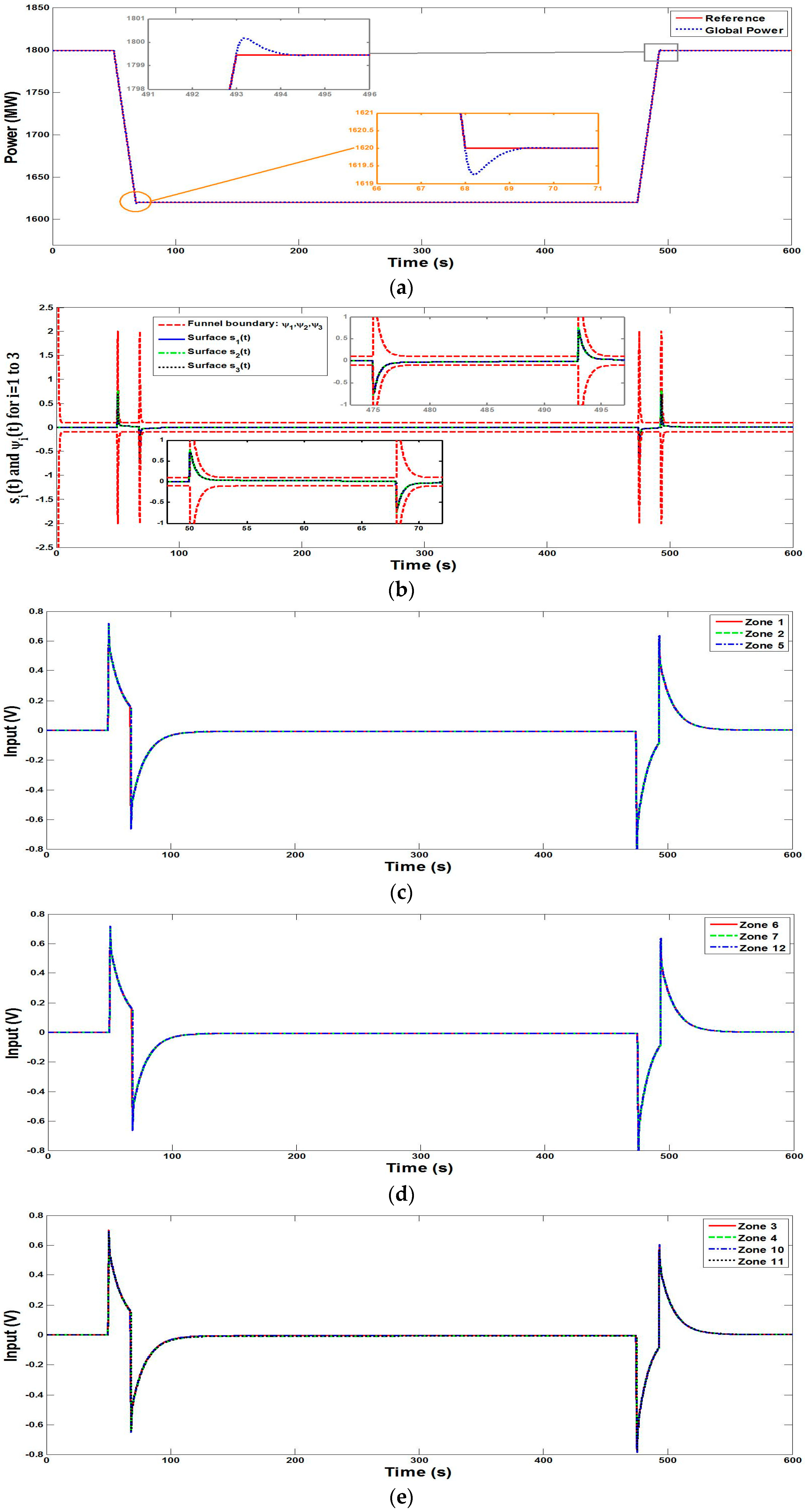
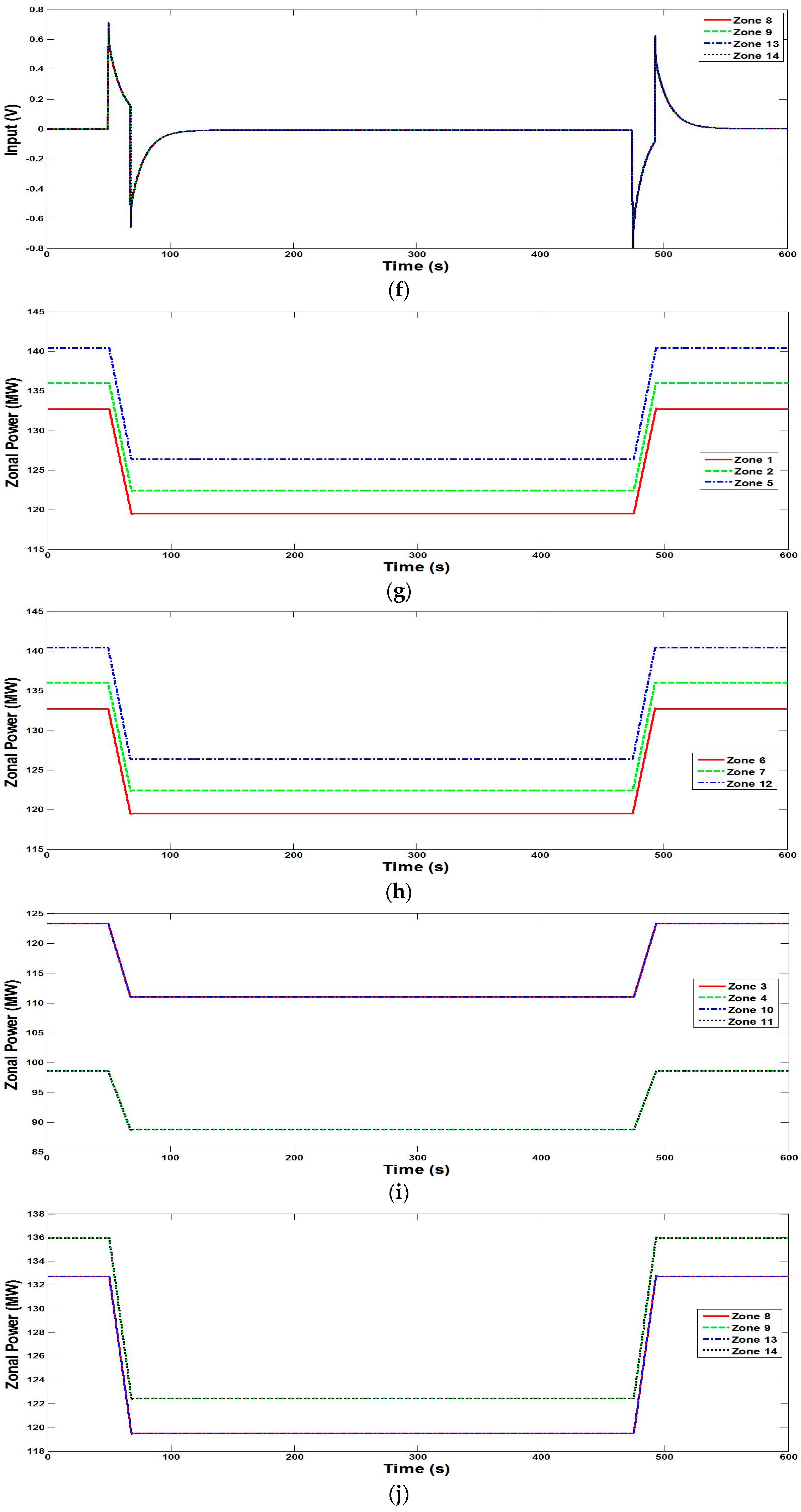
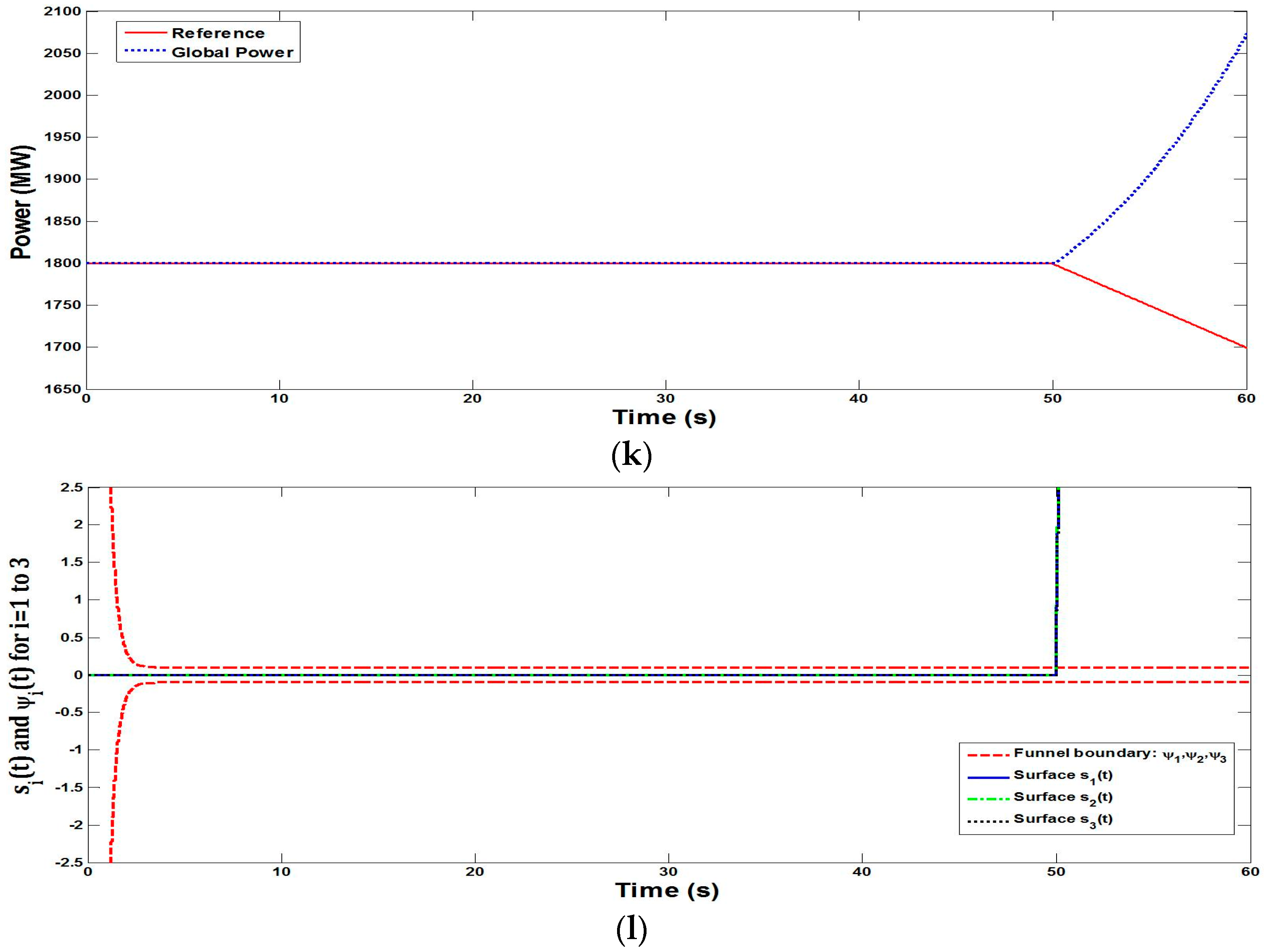
The reference-tracking capability of the proposed control scheme for the PHWR is evaluated in this scenario. For simulation, it is assumed that at $t=0 \mathrm{s}$, the reactor is operating at 100% full power (FP), that is, $z_g=1799.46 \mathrm{M}\mathrm{W}$. At $t=50 \mathrm{s}$, the power demand starts changing at a rate of −10 MW/s and attains a value of 1620 MW at $t=68 \mathrm{s}$, as shown in Figure 1a. The proposed control scheme closely follows the demanded power and adjusts the reactor global power to a new demanded power. It may be noticed in Figure 1a that the reactor global power attains a minimum of 1619.3 MW before settling at 1620 MW, whereas it has been reported in [5] and [8] that the reactor power, respectively, goes to a minimum of 1613 MW and 1611 MW before settling at 1620 MW. Furthermore, the proposed control scheme settles the reactor power to the demanded power in about 1 s, whereas the control schemes proposed in [5,8] require around 3000 s. It is further assumed that, at $t=475 \mathrm{s}$, the power demand starts to change at a rate of 10 MW/s and attains a value of 1799.46 MW at $t=493 \mathrm{s}.$ It may be noticed in Figure 1a that the proposed control scheme settles the reactor power to a value of 1799.46 MW after attaining a maximum value of 1800.2 MW. The plots of error surfaces for the first three zones, that is, $s_1\left(t\right)$ to $s_3\left(t\right)$, along with the funnel boundaries ${\psi }_1\left(t\right)$ to ${\psi }_3\left(t\right)$, are shown in Figure 1b, which shows that the error surfaces do not escape the funnel boundaries. The control signals are plotted in Figure 1c–f, whereas the zonal powers are plotted in Figure 1g–j. The plots of control signals (Figure 1c–f) depict that their amplitude remains within 1 V, whereas the amplitude of the controller signals given in [5,8] is also within 1 V and, thus, the output of the proposed controller is comparable to those of the controllers proposed in [5,8]. To demonstrate the effectiveness of the modified funnel algorithm, we also simulate the control scheme given in Equations (19)–(22) with the conventional funnel function proposed in [33,34,35], given in Equation (18). The results of the controller with the conventional funnel function are shown in Figure 1k–l. It may be observed in Figure 1l that the error surfaces escape from the funnel boundaries when the power demand at $t=50 \mathrm{s}$ changes, and, thus, the controller becomes unstable.

5.2. Scenario 2: Power Tilt

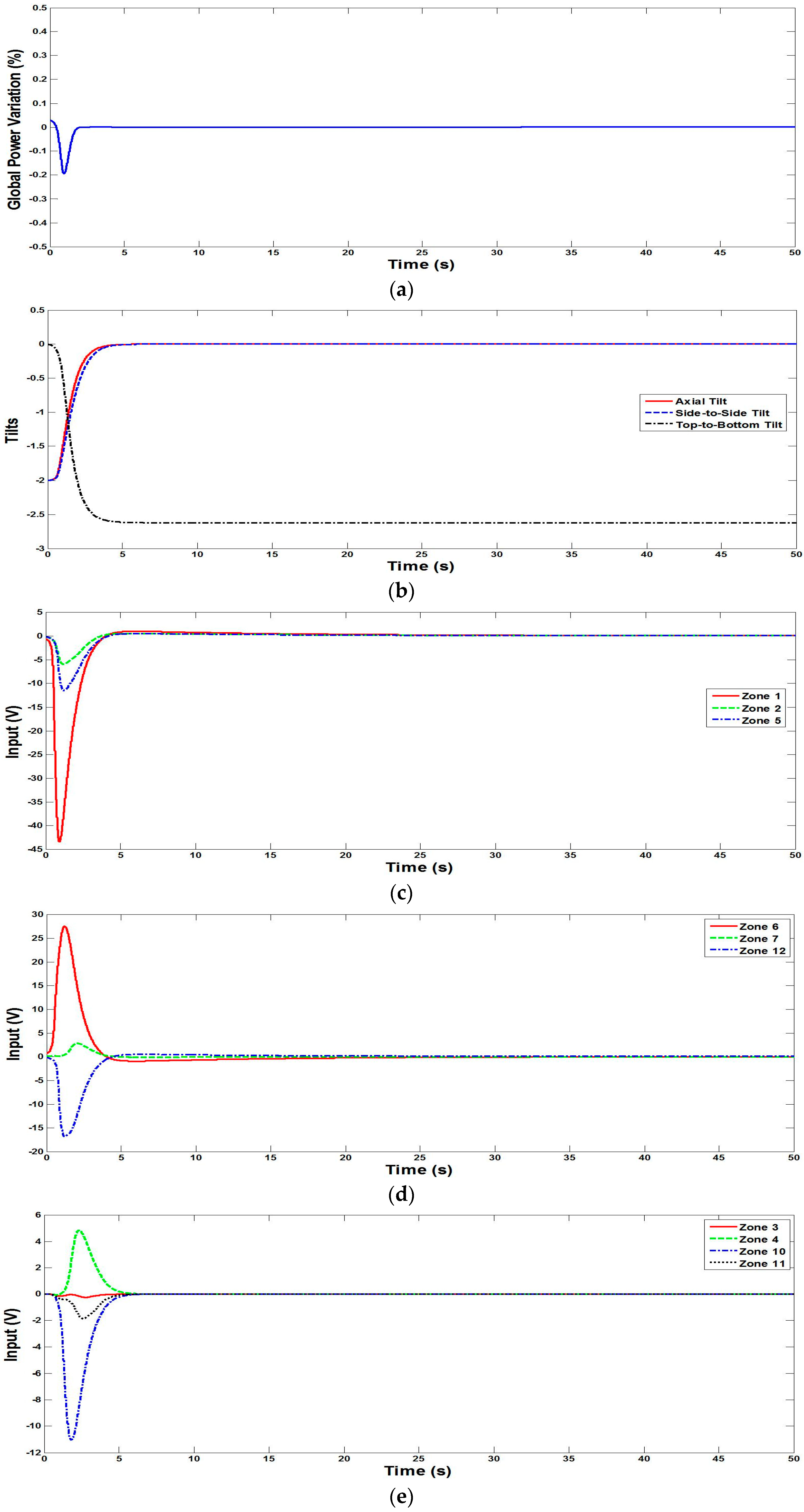
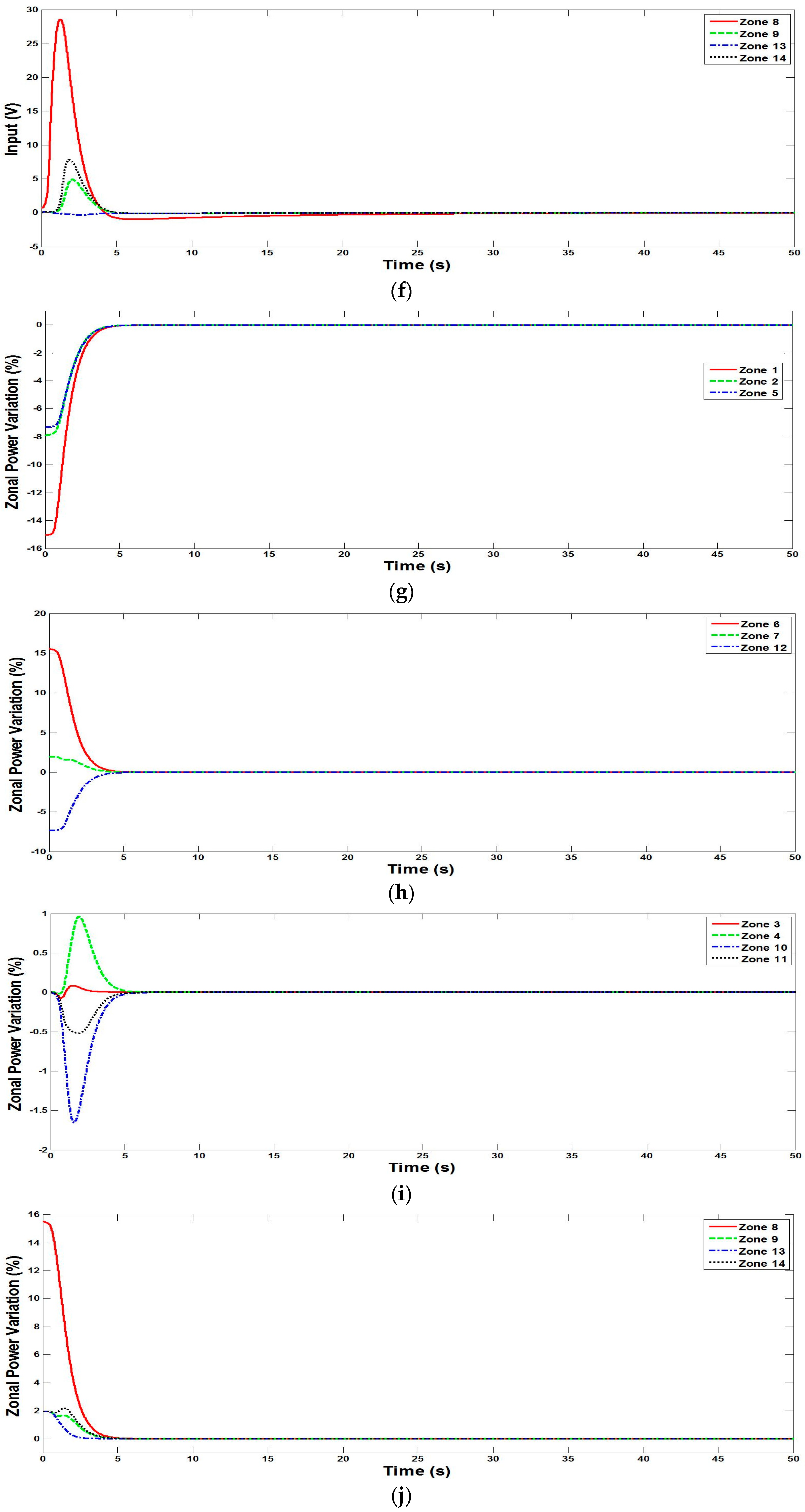
In this scenario, the capability of the proposed control scheme is evaluated for the correction of power tilts [36] of the PHWR. For simulation, it is assumed that the initial distribution of zonal power is different than the required distribution. The initial distribution, as listed in [36], is characterized by −2% side-to-side and axial tilts and 0% top-to-bottom tilt, whereas 0% side-to-side and axial tilts and around 2.5% top-to-bottom tilt are required. The transient behavior of the reactor global power is shown in Figure 2a, whereas the tilts are shown in Figure 2b. It may be noticed in Figure 2a that the absolute maximum power is about 0.19%, whereas in [5,8], around 0.45% is reported; however, a large control effort is required to achieve the results in comparison with [5,8]. Furthermore, Figure 2b depicts that the proposed control scheme corrects the tilts in about 10 s, whereas the plots of tilts in [5] and [8], respectively, depict that at least 2000 s and 3000 s are required. The controller outputs are given in Figure 2c–f, whereas the zonal powers are plotted in Figure 2g–j.

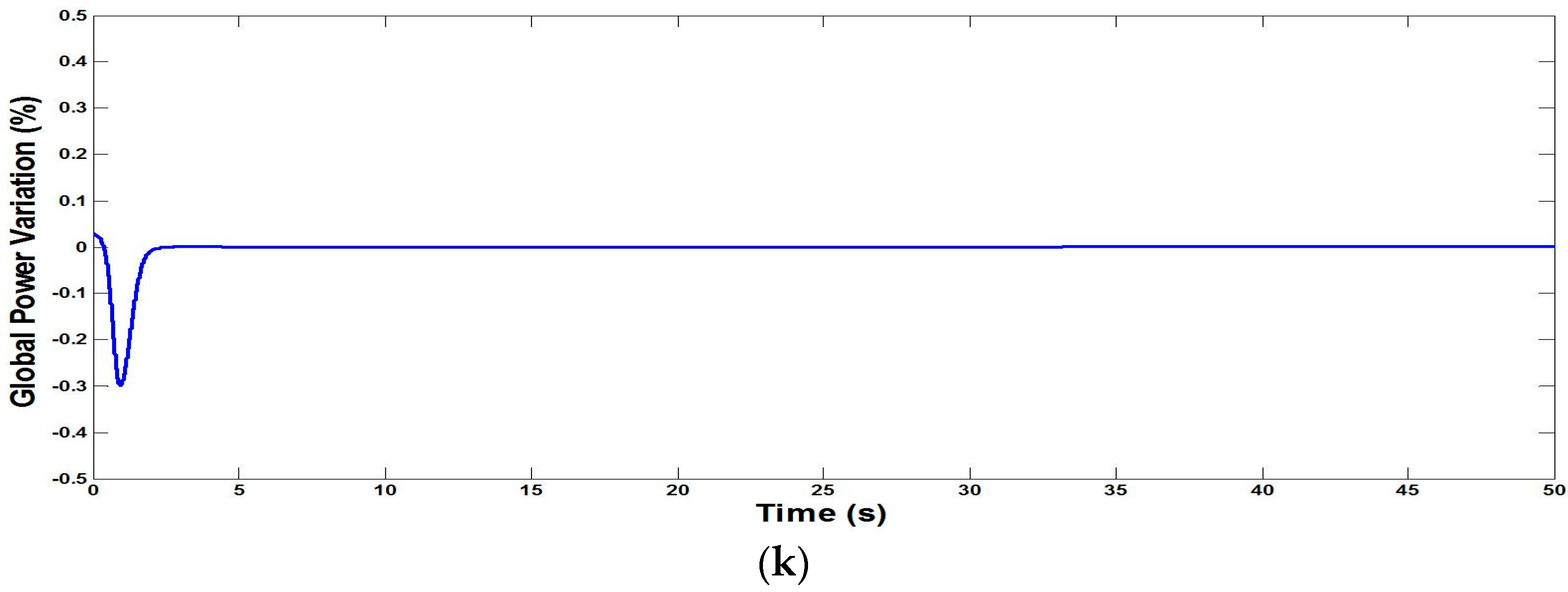
For sensitivity analysis and to study the effects of cross-coupled error terms on the system’s performance, we simulated the aforementioned scenario by changing the value of the cross-coupled parameters, that is, $c_{i,j}=0.25 \forall i\ne j$, and the resulting global power is plotted in Figure 2k. It may be noticed in Figure 2k that the global power deviation increases from 0.19% (shown in Figure 2a) to 0.3% just by changing the parameters of the cross-coupled terms.

5.3. Scenario 3: Input Disturbances

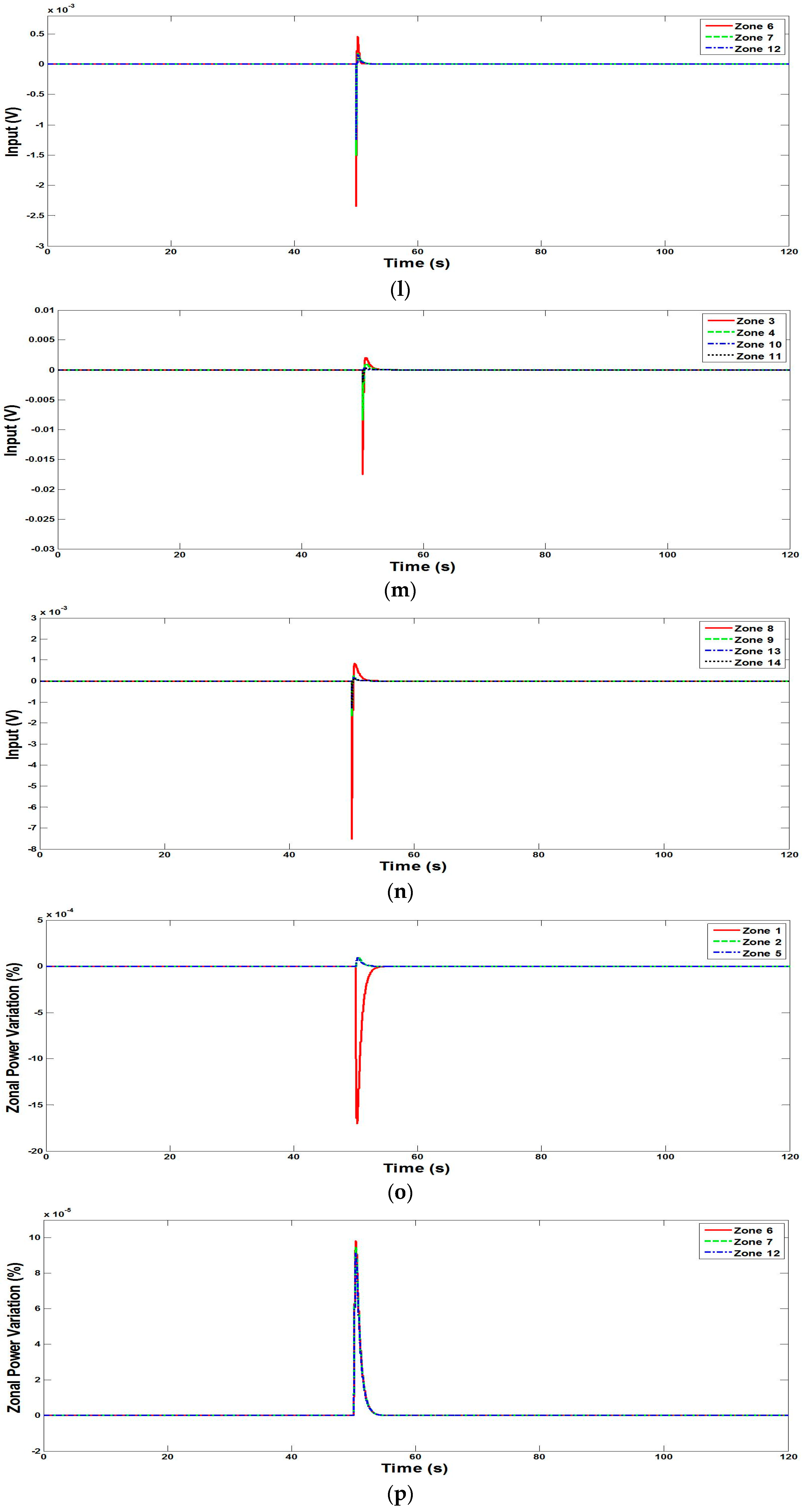
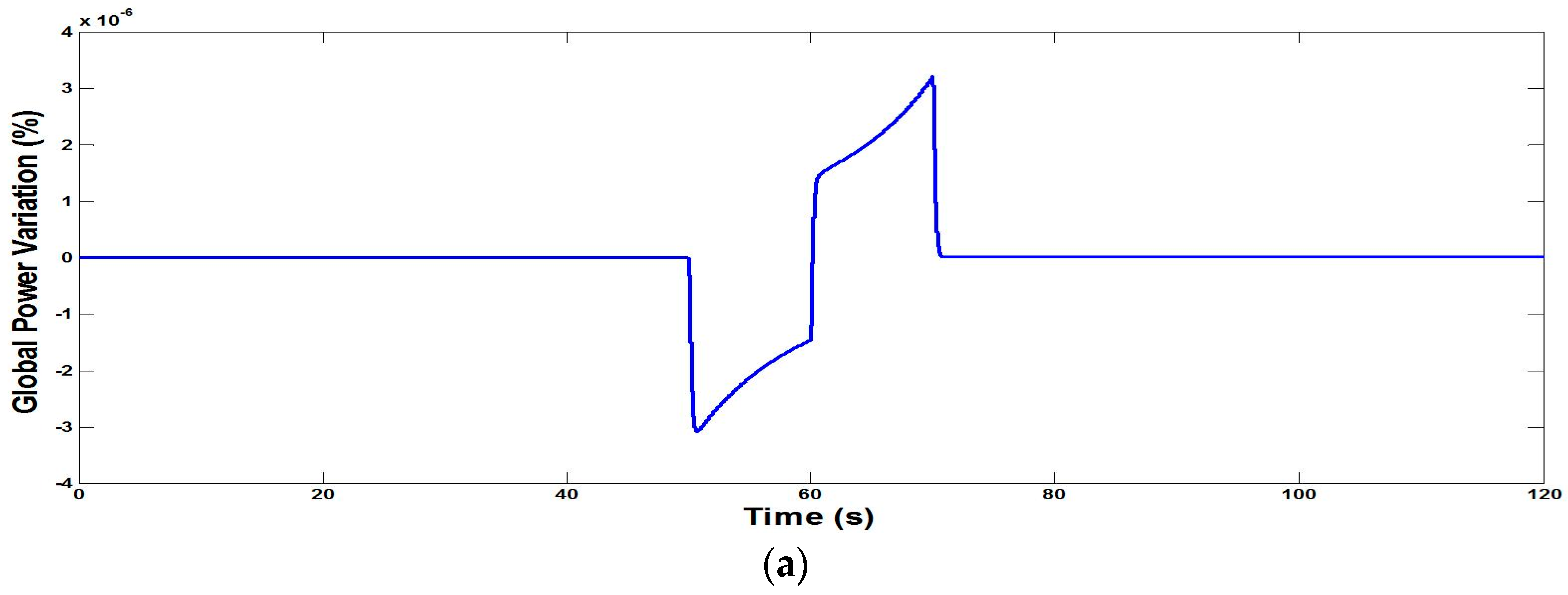
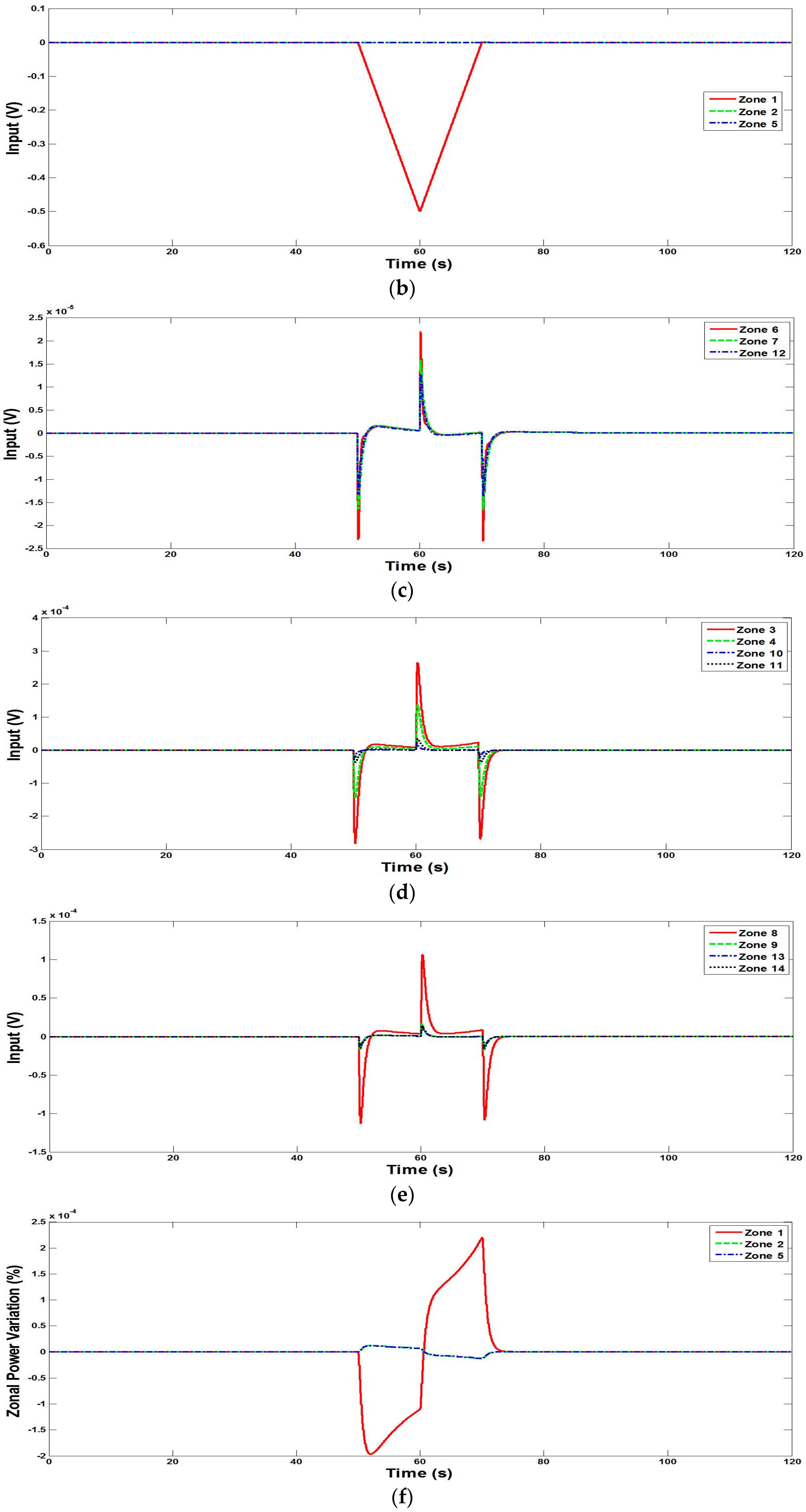
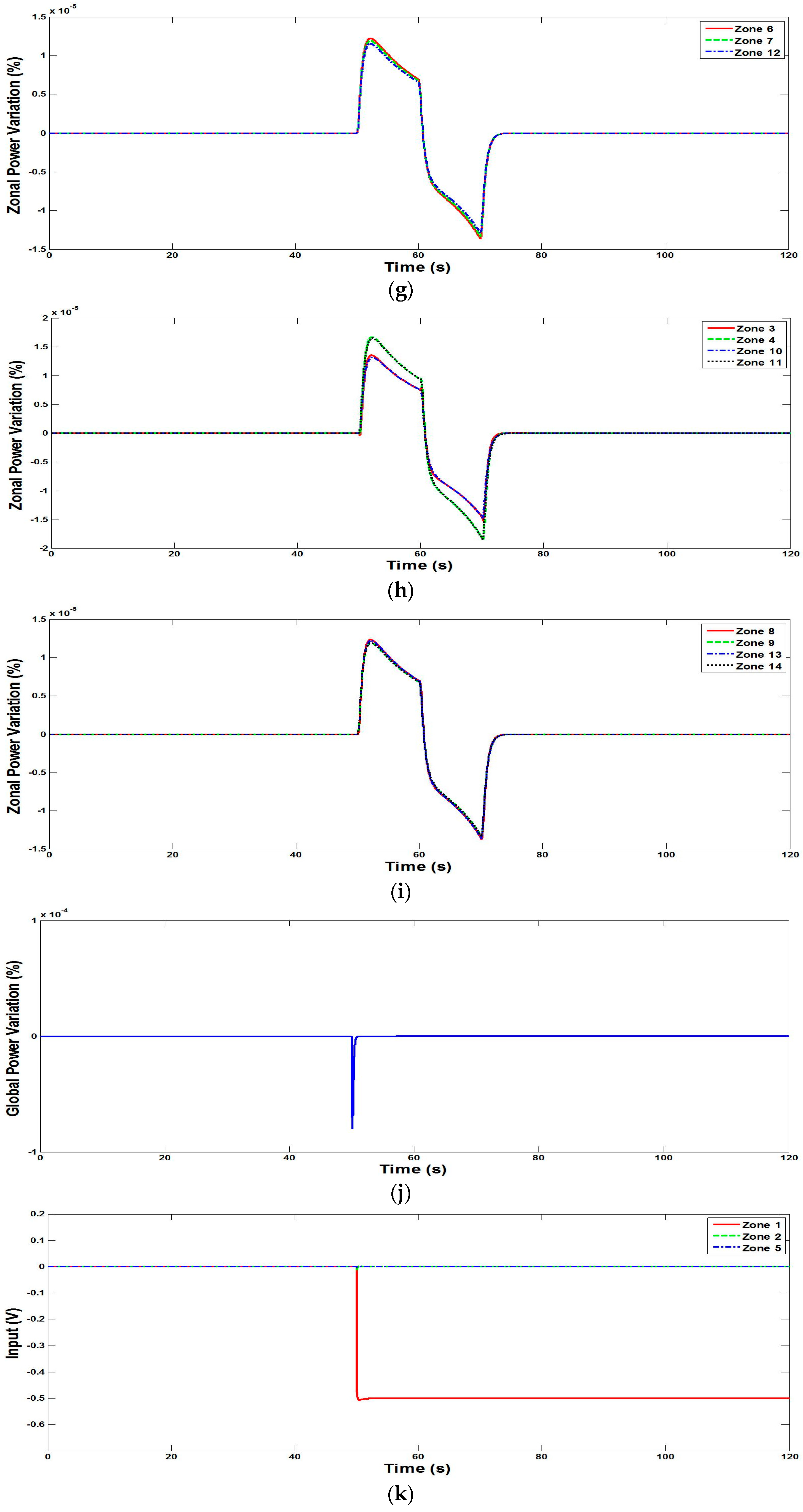
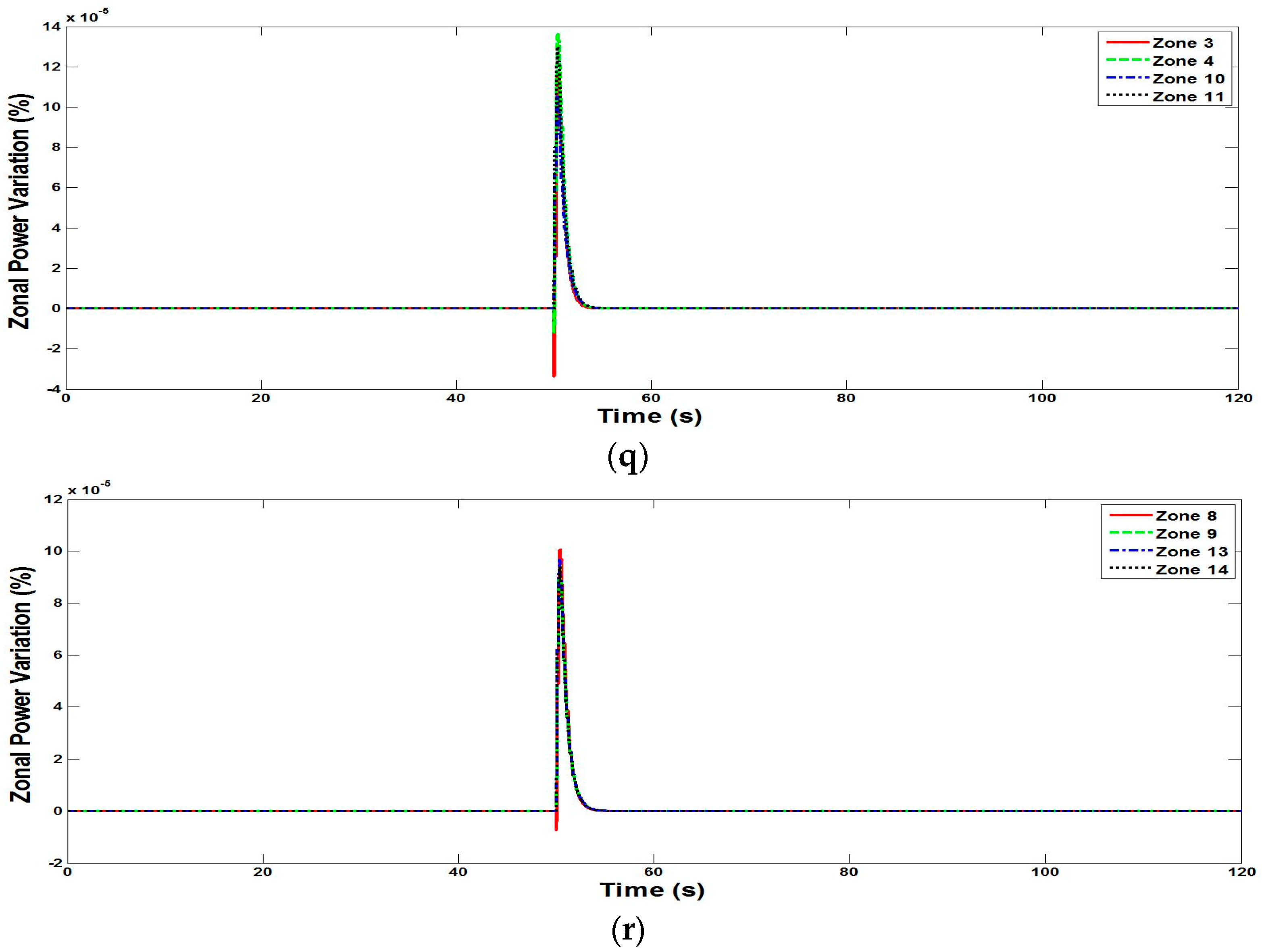
In this scenario, the robustness capability of the proposed control scheme is evaluated against the input disturbances. For simulation, it is assumed that the reactor is operating at 100% FP and the disturbance at the at the input of zone 1 of the reactor appears at $t=50 \mathrm{s}$. The input disturbance signal changes at a rate of $-0.05 \mathrm{V}/\mathrm{s}$ for 10 s, then at a rate of $0.05 \mathrm{V}/\mathrm{s}$ for the next 10 s, and then it remains at 0 thereafter. Notice that in [5], the input disturbance is assumed to vary at a lower rate, that is, 0.01 V/s (it first decreases at a rate of 0.01 V/s and then increases at the same rate for the next 10 s). The plot of reactor global power is given in Figure 3a, which shows that the absolute maximum deviation is about 0.00032 × 10⁻²%, whereas around 5 × 10⁻²% is reported in [5]. The controller outputs are given in Figure 3b–e, whereas the zonal powers are plotted in Figure 3f–i. To further investigate the robust capabilities of the proposed control scheme, a step disturbance of 0.5 V (instead of previously considered ramp input disturbance) at the input of zone 1 of the reactor is assumed to appear at $t=50 \mathrm{s}$. The plot of reactor global power is given in Figure 3j, which shows that the absolute maximum deviation is about 0.008 × 10⁻²%. The controller outputs are given in Figure 3k–n, whereas the zonal powers are plotted in Figure 3o–r. Notice that the step input disturbance scenario is not simulated in [5,8], and, therefore, we cannot comment on the stability and performance of the controllers given in [5,8].

6. Conclusions

This study presents a model-free control scheme for the load-following operation of a PHWR by proposing a modified funnel control scheme. The attractive features of the proposed control scheme are as follows: (1) the design of the controller is of low complexity, (2) the controller reduces the effects of inter-zonal coupling without using complex algorithms, and (3) the controller ensures steady-state accuracy without degrading the transient performance. For evaluating the performance of the proposed control scheme, three different scenarios (reference tracking, power tilt and input disturbances) are simulated. The simulation results show the following:

• The proposed control scheme efficiently tracks the reference signal and settles the reactor power to the demanded power in about 1 s, whereas around ±0.043% maximum overshoot/undershoot is observed.
• The proposed control scheme corrects the power tilt in about 10 s, whereas 0.19% maximum absolute deviation is observed
• The proposed control scheme effectively rejects both ramp and step input disturbances without leading the reactor to an unstable mode of operation. The maximum absolute deviation for the ramp input disturbance is about 0.00032 × 10⁻²%, whereas for the step input disturbance, it is about 0.008 × 10⁻²%.

Since the theory of funnel control (FC) is evolving, a variety of FCs, such as [25,26,28,33,34,35,37,38,39], have not considered the input constraint problem in their design. Thus, few works are available in the literature that address the problem of designing an input-constraint FC with formal theoretical support (including closed-loop stability analysis). For instance, an input constraint FC was recently proposed in [40]; however, these works have their own limitations. Furthermore, in [6,7,8,9,10,11,12,13,14,15,29,41,42], the input constraints were not considered in designing the controller, and, therefore, these works do not present formal theoretical frameworks for input-constrained control of PHWR. Likewise, we proposed a novel CCC-FC scheme for the control of a PHWR in this study; therefore, this work can be extended by considering the input constraint problem in the proposed CCC-FC scheme. Further extensions of this work include the design of an estimator to estimate the derivative terms used in the proposed controller, and the design of an adaptive version of the Cross-Coupled Conditional Funnel Controller, such that it adapts its parameters itself according to the required performance, thereby relaxing the need for the prior selection of controller parameters.

References

1. Wallam, F.; Tan, C.P. Output feedback Cross-Coupled Nonlinear PID based MIMO control scheme for Pressurized Heavy Water Reactor. J. Frankl. Inst. 2019, 356, 8012–8048. [Google Scholar] [CrossRef]
2. Ansarifar, G.R.; Akhavan, H.R. Sliding mode control design for a PWR nuclear reactor using sliding mode observer during load following operation. Ann. Nucl. Energy 2015, 75, 611–619. [Google Scholar] [CrossRef]
3. Sharma, G.L.; Bandyopadhyay, B.; Tiwari, A. Spatial control of a large pressurized heavy water reactor by fast output sampling techniques. IEEE Trans. Nucl. Sci. 2003, 50, 1740–1751. [Google Scholar] [CrossRef]
4. Talange, D.B.; Bandyopadhyay, B.; Tiwari, A. Spatial control of a large PHWR by decentralized periodic output feedback and model reduction techniques. IEEE Trans. Nucl. Sci. 2006, 53, 2308–2317. [Google Scholar] [CrossRef]
5. Reddy, G.D.; Bandyopadhyay, B.; Tiwari, A. Multirate output feedback based sliding mode spatial control for a large PHWR. IEEE Trans. Nucl. Sci. 2007, 54, 2677–2686. [Google Scholar] [CrossRef]
6. Khan, N. Decentralized State-Space Controller Design of a Large PHWR. Doctoral Dissertation, University of Ontario Institute of Technology, Oshawa, ON, Canada, 2009. [Google Scholar]
7. Khan, N.; Lu, L. A Decoupling Algorithm for Large Pressurized Heavy Water Reactors. Nucl. Technol. 2010, 172, 278–286. [Google Scholar] [CrossRef]
8. Reddy, G.D.; Park, Y.J.; Bandyopadhyay, B.; Tiwari, A.P. Discrete–time Output Feedback Sliding Mode Control of a Large Pressurized Heavy Water Reactor. IFAC Proc. Vol. 2008, 41, 8648–8653. [Google Scholar] [CrossRef]
9. Reddy, G.D.; Park, Y.J.; Bandyopadhyay, B.; Tiwari, A.P. Discrete-time output feedback sliding mode control for spatial control of a large PHWR. Automatica 2009, 45, 2159–2163. [Google Scholar] [CrossRef]
10. Munje, R.K.; Patre, B.M.; Shimjith, S.R.; Tiwari, A.P. Sliding Mode Control for Spatial Stabilization of Advanced Heavy Water Reactor. IEEE Trans. Nucl. Sci. 2013, 60, 3040–3050. [Google Scholar] [CrossRef]
11. Bhase, S.S.; Patre, B.M. Robust FOPI controller design for power control of PHWR under step-back condition. Nucl. Eng. Des. 2014, 274, 20–29. [Google Scholar] [CrossRef]
12. Patre, B.M.; Londhe, P.S.; Nagarale, R.M. Fuzzy Sliding Mode Control for Spatial Control of Large Nuclear Reactor. IEEE Trans. Nucl. Sci. 2015, 62, 2255–2265. [Google Scholar] [CrossRef]
13. Surjagade, P.V.; Tiwari, A.P.; Shimjith, S.R. Robust Optimal Integral Sliding Mode Controller for Total Power Control of Large PHWRs. IEEE Trans. Nucl. Sci. 2018, 65, 1331–1344. [Google Scholar] [CrossRef]
14. Desai, R.J.; Patre, B.M.; Munje, R.K.; Tiwari, A.P.; Shimjith, S.R. Integral Sliding Mode for Power Distribution Control of Advanced Heavy Water Reactor. IEEE Trans. Nucl. Sci. 2020, 67, 1076–1085. [Google Scholar] [CrossRef]
15. Singh, R.; Dora, T.; Lamba, R.; Bhullar, A.; Sondhi, S. FOPID controller design for a perturbed PHWR system using enhanced crow search algorithm. Prog. Nucl. Energy 2022, 151, 104342. [Google Scholar] [CrossRef]
16. Khalil, H.K. Nonlinear Systems, 3rd ed.; Prentice Hall: Hoboken, NJ, USA, 2002. [Google Scholar]
17. Ansarifar, G.R.; Saadatzi, S. Sliding Mode Control for Pressurized-Water Nuclear Reactors in load following operations with bounded xenon oscillations. Ann. Nucl. Energy 2015, 76, 209–217. [Google Scholar] [CrossRef]
18. Yadava, D.K.; Gupta, A.; Munshi, P. Design of NDI-SMC based robust hybrid nonlinear controller for load following operation in pressurized water reactor. Nucl. Eng. Des. 2020, 363, 110604. [Google Scholar] [CrossRef]
19. Davijani, N.Z.; Jahanfarnia, G.; Abharian, A.E. Nonlinear Fractional Sliding Mode Controller Based on Reduced Order FNPK Model for Output Power Control of Nuclear Research Reactors. IEEE Trans. Nucl. Sci. 2017, 64, 713–723. [Google Scholar] [CrossRef]
20. Abdulraheem, K.K.; Korolev, S.A. Robust optimal-integral sliding mode control for a pressurized water nuclear reactor in load following mode of operation. Ann. Nucl. Energy 2021, 158, 108288. [Google Scholar] [CrossRef]
21. Wallam, F.; Abbas, A.; Abbasi, A.R. Design and tuning of a Decentralized Fuzzy Logic Controller for a MIMO type Pressurized Heavy Water Reactor. Ann. Nucl. Energy 2015, 85, 1104–1114. [Google Scholar] [CrossRef]
22. Wallam, F.; Abbasi, A.R. Evaluating the Transient Handling Capability of a Fuzzy Logic Controller for a Pressurized Heavy Water Reactor. J. Control Eng. Appl. Inform. 2014, 16, 40–48. [Google Scholar]
23. Pravosud, S.S.; Maslakov, D.S.; Yakubov, Y.O. Application of Fuzzy Controllers for Power Control of the VVER-1200 Nuclear Reactor. Math. Model. Nucl. Technol. 2024, 87, 1430–1439. [Google Scholar] [CrossRef]
24. Khandekar, A.A.; Patre, B.M. Design and application of discrete sliding mode controller for TITO process control systems. In Advances and Applications in Sliding Mode Control Systems; Springer: Cham, Switzerland, 2015; pp. 255–277. [Google Scholar]
25. Ilchmann, A.; Ryan, E.P.; Sangwin, C.J. Tracking with prescribed transient behavior. ESAIM Control Optim. Calc. Var. 2002, 7, 471–493. [Google Scholar] [CrossRef]
26. Wallam, F.; Memon, A.Y.; Tan, C.P. Shifting Funnel Control: A Model-Free Approach for Load Following Operation of PWR. Nucl. Technol. 2025. [Google Scholar] [CrossRef]
27. Seshagiri, S.; Khalil, H.K. Robust output feedback regulation of minimum-phase nonlinear systems using conditional integrators. Automatica 2005, 41, 43–54. [Google Scholar]
28. Wallam, F.; Memon, A.Y.; Tan, C.P. Conditional Funnel Control: A Simple Approach to Prescribed Performance Asymptotic Tracking and its Industrial Applications. Trans. Inst. Meas. Control 2025. [Google Scholar] [CrossRef]
29. Vaswani, P.D.; Tamboli, P.K.; Chakraborty, D. Optimized FSF Controller for Bulk Power Control of Large-Core PHWRs. Nucl. Technol. 2024, 210, 126–136. [Google Scholar] [CrossRef]
30. Tiwari, A.P. Modeling and Control of a Large Pressurized Heavy Water Reactor. Ph.D. Dissertation, Indian Institute of Technology, India, 1999. [Google Scholar]
31. Edwards, R.M.; Lee, K.Y.; Ray, A. Robust optimal control of nuclear reactors and power plants. Nucl. Technol. 1992, 98, 137–148. [Google Scholar] [CrossRef]
32. Wallam, F.; Memon, A.Y. A robust control scheme for nonlinear non-isothermal uncertain jacketed continuous stirred tank reactor. J. Process Control 2017, 51, 55–67. [Google Scholar] [CrossRef]
33. Hackl, M.C.; Hopfe, N.; Ilchmann, A.; Mueller, M.; Trenn, S. Funnel control for systems with relative degree two. SIAM J. Control Optim. 2013, 51, 965–995. [Google Scholar] [CrossRef]
34. Chowdhury, D.; Khalil, H.K. Funnel control for nonlinear systems with arbitrary relative degree using high-gain observers. Automatica 2019, 105, 107–116. [Google Scholar] [CrossRef]
35. Berger, T.; Lê, H.H.; Reis, T. Funnel control for nonlinear systems with known strict relative degree. Automatica 2018, 87, 345–357. [Google Scholar] [CrossRef]
36. Doshi, J.B.; Obaidurrahman. Control of Spatial Xenon Oscillations in Large Power Reactors. In Proceedings of the Advances in Nuclear Analysis and Simulation PHYSOR, Vancouver, BC, Canada, 10–14 September 2006. [Google Scholar]
37. Gao, R.-B.; Zhang, X.; Ahn, H.-S.; Antonis, V. Global Funnel Control of Nonlinear Systems with Unknown and Time-Varying Fractional Powers. Fractal Fract. 2025, 9, 648. [Google Scholar] [CrossRef]
38. Zhang, J.-X.; Chai, T. Proportional-Integral Funnel Control of Unknown Lower-Triangular Nonlinear Systems. IEEE Trans. Autom. Control 2024, 69, 1921–1927. [Google Scholar] [CrossRef]
39. Ait-Chekdhidh, Z.; Ardjal, A.; Bettayeb, M. Funnel control based super-twisting sliding mode control of wind turbines. J. King Saud Univ. Eng. Sci. 2025, 37, 25. [Google Scholar] [CrossRef]
40. Berger, T. Input-Constrained Funnel Control of Nonlinear Systems. IEEE Trans. Autom. Control 2024, 69, 5368–5382. [Google Scholar] [CrossRef]
41. Londhe, P.S.; Patre, B.M.; Tiwari, A.P. Fuzzy-like PD controller for spatial control of advanced heavy water reactor. Nucl. Eng. Des. 2014, 274, 77–89. [Google Scholar] [CrossRef]
42. Banerjee, S.; Halder, K.; Dasgupta, S.; Mukhopadhyay, S.; Ghosh, K.; Gupta, A. An interval approach for robust control of a large PHWR with PID controllers. IEEE Trans. Nucl. Sci. 2015, 62, 281–292. [Google Scholar] [CrossRef]
Figure 1. Scenario 1. (a) Plot of reactor global power and demanded power for the proposed scheme. (b) Plot of s i t and ψ i t (i = 1 to 3) for the proposed scheme. (c) Plot of controller outputs for zones 1, 2 and 5. (d) Plot of controller outputs for zones 6, 7 and 12. (e) Plot of controller outputs for zones 3, 4, 10 and 11. (f) Plot of controller outputs for zones 8, 9, 13 and 14. (g) Plot of power for zones 1, 2 and 5. (h) Plot of power for zones 6, 7 and 12. (i) Plot power for zones 3, 4, 10 and 11. (j) Plot of power for zones 8, 9, 13 and 14. (k) Plot of reactor global power and demand power for the funnel function given in Equation (18). (l) Plot of s i t and ψ i t (i = 1 to 3) for the funnel function given in Equation (18).
Eng 07 00226 g001aEng 07 00226 g001bEng 07 00226 g001c
Figure 2. Scenario 2. (a) Plot of global power variation. (b) Plot of axial, side-to-side and top-to-bottom tilts. (c) Plot of controller outputs for zones 1, 2 and 5. (d) Plot of controller outputs for zones 6, 7 and 12. (e) Plot of controller outputs for zones 3, 4, 10 and 11. (f) Plot of controller outputs for zones 8, 9, 13 and 14. (g) Plot of power for zones 1, 2 and 5. (h) Plot of power for zones 6, 7 and 12. (i) Plot power for zones 3, 4, 10 and 11. (j) Plot of power for zones 8, 9, 13 and 14. (k) Plot of global power variation for c i , j = 0.25     i j .
Eng 07 00226 g002aEng 07 00226 g002bEng 07 00226 g002c
Figure 3. Scenario 3. (a) Plot of global power variation for ramp input disturbance. (b) Plot of controller outputs for zones 1, 2 and 5 for ramp input disturbance. (c) Plot of controller outputs for zones 6, 7 and 12 for ramp input disturbance. (d) Plot of controller outputs for zones 3, 4, 10 and 11 for ramp input disturbance. (e) Plot of controller outputs for zones 8, 9, 13 and 14 for ramp input disturbance. (f) Plot of power for zones 1, 2 and 5 for ramp input disturbance. (g) Plot of power for zones 6, 7 and 12 for ramp input disturbance. (h) Plot power for zones 3, 4, 10 and 11 for ramp input disturbance. (i) Plot of power for zones 8, 9, 13 and 14 for ramp input disturbance. (j) Plot of global power variation for step input disturbance. (k) Plot of controller outputs for zones 1, 2 and 5 for step input disturbance. (l) Plot of controller outputs for zones 6, 7 and 12 for step input disturbance. (m) Plot of controller outputs for zones 3, 4, 10 and 11 for step input disturbance. (n) Plot of controller outputs for zones 8, 9, 13 and 14 for step input disturbance. (o) Plot of power for zones 1, 2 and 5 for step input disturbance. (p) Plot of power for zones 6, 7 and 12 for step input disturbance. (q) Plot power for zones 3, 4, 10 and 11 for step input disturbance. (r) Plot of power for zones 8, 9, 13 and 14 for step input disturbance.
Eng 07 00226 g003aEng 07 00226 g003bEng 07 00226 g003cEng 07 00226 g003dEng 07 00226 g003e
Disclaimer/Publisher’s Note: The statements, opinions and data contained in all publications are solely those of the individual author(s) and contributor(s) and not of MDPI and/or the editor(s). MDPI and/or the editor(s) disclaim responsibility for any injury to people or property resulting from any ideas, methods, instructions or products referred to in the content.