Article

Characterization of Cavity Reservoirs Based on a Shape-Constrained Multi-Trace Seismic Inversion Method


1
SINOPEC Geophysical Research Institute Co., Ltd., Nanjing 211103, China
2
School of Geoscience and Technology, Southwest Petroleum University, Chengdu 610500, China
*
Author to whom correspondence should be addressed.
Eng 2026, 7(5), 222; https://doi.org/10.3390/eng7050222
Submission received: 31 March 2026 / Revised: 30 April 2026 / Accepted: 4 May 2026 / Published: 7 May 2026

Abstract

Ultra-deep marine carbonate cavity reservoirs in Northwest China are characterized by strong heterogeneity and complex geometries. Conventional seismic inversion methods generate over-smoothed results, blur geological boundaries, and suffer from severe non-uniqueness, making it difficult to accurately identify low-impedance cavity anomalies. To tackle these problems, this study develops a shape-constrained multi-trace seismic inversion method based on the Mumford–Shah functional. To meet the computational requirements, a multi-trace inversion framework is adopted, and the Ambrosio–Tortorelli approximation is introduced to convert the non-smooth Mumford–Shah functional into a solvable smooth form. The proposed method realizes the joint inversion of acoustic impedance and geological interfaces, implicitly encourages piecewise constant regions and preserves sharp geological boundaries, and effectively mitigates inversion non-uniqueness. Numerical experiments and field applications validate that the method delivers high lateral resolution and boundary accuracy even with limited prior information and reliably delineates discrete “string-bead” cavity geometries with high consistency to drilling and logging data, providing a robust solution for fine characterization of complex carbonate cavity reservoirs.

1. Introduction

Carbonate reservoirs are widely distributed in the Tarim Basin, Northwest China. The burial depth of these reservoirs exceeds 6500 m [1]. Along strike-slip fault zones, multi-stage tectonic fracturing has driven the development of caves, pores, and fracture-type reservoirs within carbonate strata [2,3]. Carbonate reservoirs, particularly cavity reservoirs, present substantial exploration challenges. Such cavity reservoirs are the key drilling targets for achieving prolific oil and gas wells in production [4]. Having undergone intense late-stage transformation, carbonate cavity reservoirs are characterized by strong heterogeneity, diverse reservoir types, discrete spatial distribution, and combinations [5]. These characteristics result in complex seismic responses of the target interval, posing great challenges to reservoir interpretation.
Using a characteristic seismic reflection pattern known as the “string-bead responses (SBRs)”, seismic imaging can identify the development extent of karst cavities within carbonate strata [6]. However, owing to the limited bandwidth of seismic wavelets and interference between reflection events, the seismic imaging lacks detailed information on morphology, boundaries, and combination types of the cavities. In the early stages of exploration, seismic attribute techniques are widely used [7]. This method typically adopts the integrated application of multiple seismic attributes, including seismic coherence, ant-tracking attributes, gradient structure tensor (GST), reflection intensity, and root mean square (RMS) amplitude, and has yielded numerous successful field applications in fault-controlled cavity reservoir prediction [8,9,10,11]. Attribute methods require higher-quality seismic data (signal-to-noise ratio and resolution of seismic data) and are mostly used to qualitatively characterize the extent of fractured zones in fault-controlled reservoirs. Moreover, amplitude-based attributes cannot resolve the blurring effects caused by wavelets in the seismic response of cavity reservoirs, and the identification of reservoir boundaries requires thresholds based on statistical attribute values from confirmed reservoirs that have been validated through drilling [12].
One-dimensional sparse pulse inversion with prior constraints based on seismic data has been widely used to estimate subsurface impedance models and has also been applied in carbonate reservoirs. However, conventional seismic inversion methods primarily rely on relatively homogeneous low-frequency models to predict reservoir parameters [13,14,15]. In practical exploration, constructing a reliable prior model for carbonate cavity reservoirs poses major difficulties. The strong heterogeneity of carbonate cavity reservoirs leads to significant lateral energy variations in their seismic responses. Furthermore, during drilling operations, severe circulation losses often occur when the drill string traverses reservoir formations within the target interval. These downhole anomalies not only compromise the operational stability of the logging string but also result in a severe shortage of valid logging curve data for reservoir evaluation [16,17]. These factors lead to the inaccuracy of the constructed prior model. When applying conventional inversion methods, if the prior constraints are insufficient, a large number of isolated and laterally abrupt banded anomalies will appear in the inversion profile, which are generated by the inherent limitations of the single-trace seismic inversion method. Conversely, strong constraints built upon an unreliable prior model can mask low-impedance anomalies, which reduces the effectiveness of oil and gas exploration [18]. Subsequent geostatistical inversion and facies-controlled inversion have also been applied to carbonate cavity reservoirs. However, these methods still rely heavily on the quality of seismic attributes or seismic facies that constrain the inversion, resulting in inconsistent accuracy of the inversion results [19,20]. Additionally, the recent development of full-waveform inversion (FWI) and artificial intelligence has also driven progress in seismic inversion and fracture-cavity characterization. However, FWI is computationally prohibitive, especially for ultra-deep carbonate reservoirs, since high-resolution inversion requires extremely large computational resources [21]. Although machine learning-based inversion methods achieve encouraging improvements for conventional reservoirs, the lack of sufficient real field data for training remains a key factor limiting their application to ultra-deep cavity reservoirs [12,22,23]. Therefore, the practical performance of these methods on real ultra-deep carbonate cavity datasets still needs further investigation and development.
To address the limitations of single-trace inversion, recent studies have increasingly focused on multi-trace impedance inversion. Unlike single-trace seismic inversion, the inherent nature of multi-trace synchronous inversion avoids spurious lateral anomalies in the inversion results [24,25]. Meanwhile, multi-trace inversion takes 2D or 3D models as both input and output, allowing us to incorporate spatial constraints or structural regularization to achieve the desired inversion performance [26]. In recent years, multi-trace inversion methods have been significantly improved to address nonstationary seismic effects and regularization challenges. Advanced multi-trace inversion incorporates structural constraints to achieve simultaneous estimation of attenuation parameters and reflectivity, enhancing both temporal resolution and spatial structural continuity [27]. Adaptive multiplicative regularization strategies have also been developed for multi-trace inversion, enabling automatic adjustment of regularization strength and avoiding inefficient manual parameter tuning [28]. These developments promote more stable, high-resolution, and structurally consistent impedance results for complex geological environments.
From the perspective of methodological essence, geostatistical inversion focuses on reproducing statistical spatial variability, facies-controlled inversion emphasizes geological constraint consistency under predefined facies boundaries, and multi-trace inversion aims to enhance lateral structural continuity by leveraging structural similarity among adjacent traces. Although these three categories of methods improve the stability and geological rationality of inversion results, they essentially pursue continuous or smoothly varying parameter fields, which are inherently inconsistent with the discrete, isolated, and strongly heterogeneous characteristics of carbonate cavity reservoirs.
For cavity-type reservoirs, our objective is to highlight the low-impedance anomalies corresponding to discrete high-energy “string-bead” responses and recover their accurate geometries. This task is mathematically analogous to image segmentation, which aims to identify piecewise constant regions and discontinuous boundaries [29]. In contrast to conventional inversion paradigms, image segmentation provides a natural and powerful alternative that aligns perfectly with the goal of characterizing sharp, isolated cavity reservoirs.
As a classical variational model for image segmentation, the Mumford–Shah (MS) functional can simultaneously realize intra-region smoothing and inter-region boundary preservation, thus providing a rigorous theoretical bridge between seismic inversion and cavity shape characterization. Image segmentation is a fundamental topic in computer vision, which typically uses the gradient information of model parameters to delineate boundaries of different structural units. As the representative variational model for free-discontinuity problems, the MS functional achieves image segmentation, denoising, and reconstruction by capturing internal structural and interface features [30]. This analogy motivates us to introduce the MS functional into multi-trace seismic inversion.
In this paper, we propose a shape-constrained multi-trace seismic inversion method based on the MS functional. The key innovation of the shape-constrained inversion method is the simultaneous inversion of interfaces and parameter values. Implicit shape representation is achieved based on the MS functional framework. Within this framework, implicit shape representation forms a sharp transition layer only at true interfaces, thereby avoiding the common pitfall of conventional inversion methods that sacrifice structural clarity to reduce data misfit. By implicitly encouraging piecewise constant regions, this framework effectively reduces excessive degrees of freedom in the optimization process.
By imposing shape constraints, the inversion results of strongly inhomogeneous reservoirs achieve higher spatial resolution and reservoir prediction accuracy. We first validate the proposed method using synthetic data. Numerical tests indicate that shape-constrained inversion offers significant advantages for structural reconstruction and also provides higher numerical accuracy for wave impedance when prior information is limited. We further apply the method to real seismic data acquired over carbonate cavity reservoirs in northwestern China. Field applications demonstrate that the proposed method provides substantially better characterization of cavity-type reservoirs than conventional approaches.
To explicitly summarize the main contributions of this work, three key innovations are highlighted as follows: First, a shape-constrained multi-trace inversion strategy embedded with the MS functional is proposed to realize the joint inversion of geological interfaces and subsurface parameters. Second, implicit shape representation is introduced to address the strong inhomogeneity of carbonate cavity reservoirs, which ensures sharp boundary preservation while reducing optimization complexity. Third, the proposed method effectively avoids the trade-off between structural clarity and data misfit existing in conventional methods and reduces empirical parameter tuning, thus improving the practicality and reliability of high-resolution reservoir characterization.

2. Theory and Methods

In this chapter, we first introduce the basic principles of multi-trace seismic inversion. On this basis, we incorporate the Mumford–Shah functional as a regularization term to establish the objective function for shape-constrained multi-trace inversion. We also present the corresponding solution method and the workflow for applying the proposed approach.

2.1. Multi-Trace Impedance Inversion

Single-trace post-stack seismic traces follow the convolutional model [31]:
S = W R + n .
where S is a vector of single-trace seismic record, W is a wavelet matrix, R is a vector of reflectivity series, and n denotes noise signal. The symbol * in the equation indicates the convolution operation. We write the impedance of a layer in the time domain as z i , and the impedance of its adjacent next layer as z i + 1 , then the reflectivity r i can be written as [32]:
r i = ( z i + 1 z i ) / ( z i + 1 + z i ) .
In general, the acoustic impedance contrast between adjacent strata is weak. To facilitate the linearization of the formulated equation, the relationship between impedance and reflection coefficient can be approximated for linearization [33]:
r i ( ln z i + 1 ln z i ) / 2 .
Thus, under noise-free conditions, Equation (1) can be rewritten in matrix form:
s 1 s 2 s n 1 S = 1 2 w 1 0 0 w 1 w k 0 0 w k   w 1 0 0 w k 1 1 0 0 0 1 1 0 0 0 1 1 A ln z 1 ln z 2 ln z n X , S = A X .
where s is the seismic amplitude, w means the wavelet, k is the length of the wavelet, A is the forward modeling operator, X is the impedance vector. Equation (4) is a single-trace forward function, and we can obtain a multi-trace forward function by expanding vectors S and X into two-dimensional matrices:
S 1 , S 2 , , S m D = A [ X 1 , X 2 , , X m ] M .
where m is the trace number, S m is the m-th seismic signal trace of data, X m is the m-th impedance trace of the model. Hence, D is the seismic signal matrix, M is the impedance model matrix, they both include m traces. Based on the multi-trace forward modeling operator, we can easily derive the objective function of multi-trace inversion by the least squares method:
min f ( M ) = D o b A M 2 2 .
where D o b is the observation seismic data, and   2 means the L2 norm. The gradient is obtained by differentiating the objective function:
δ M = ( A T A ) 1 A T ( D o b A M ) .
In this study, multi-trace inversion is adopted for two main reasons. First, simultaneous multi-trace inversion can enhance the lateral coherence of the inverted results. Second, the shape-constrained inversion method introduced subsequently cannot effectively capture structural information of the model in a single-trace framework. Therefore, a multi-trace inversion strategy is necessary.

2.2. Shape-Constrained Inversion

Regularization is essential for stabilizing seismic inversion and imposing geologically reasonable constraints on subsurface parameter distributions. Tikhonov L2 regularization with initial-model constraints is one of the most widely used regularization strategies [34]:
r T i k h o n o v ( m ) = α m m 0 2 2 .
where m is the model parameter, m 0 is the prior model, α is the weighting factor to control the strength of the constraint.
Physically, this term forces the inverted model to conform to the prior model and suppresses numerical oscillations. However, it enforces global smoothness across the entire model domain, which directly contradicts the physical characteristics of ultra-deep carbonate cavity reservoirs: discrete spatial distribution, strong impedance discontinuities at cavity boundaries, and non-layered depositional environments. In addition, borehole collapse is a common occurrence in ultra-deep fractured carbonate rocks, resulting in significantly increased borehole wall roughness or a marked expansion of the borehole diameter. These adverse drilling conditions lead to missing density, compressional seismic, and neutron logging data, leaving the model without sufficient prior information [18].
To resolve this physical mismatch, we introduce the MS functional—a variational model originally developed for image segmentation that naturally preserves discontinuities at structural boundaries. Mathematically and geophysically, the sharp impedance boundaries between carbonate cavities and host rocks are analogous to the interfaces in image processing. The MS functional partitions the subsurface into distinct geo-bodies separated by sharp interfaces, enforcing smooth parameter variations within each geo-body while allowing strong contrasts across interfaces. This design is physically consistent with the actual distribution of cavity reservoirs. The MS functional is defined as [30]:
f M S ( i , K ) = Ω m g 2 d x + α Ω \ K m 2 d x + β K d χ .
where m is the data to be updated, g is the observation data, Ω is the spatial space of the target model and K is the interface set. The MS functional can be decomposed into three contribution terms. The first term in Equation (9) serves to reduce the discrepancy between the simulated and observed data. The second term is a penalization of parameter variation in the model space other than the interface set K . And the third integral term measures arclength and penalizes oscillations of interfaces. The two coefficients, α and β , serve as weighting factors to balance the contributions of the last two terms.
The MS functional partitions the model into distinct subregions, enforces parameters to be smooth within each region, and regularizes the length of interfaces [30]. In other words, when applied to subsurface parameter inversion, the MS functional facilitates the segmentation of the domain into multiple, distinct regions and their corresponding interfaces. Crucially, it permits significant spatial variations in parameters across different regions, thereby preventing the suppression of low-impedance anomalies associated with cavity reservoirs. However, it is difficult to minimize Equation (9) owing to the unknown interface set K . Although the Mumford–Shah functional provides an ideal mathematical framework for shape-constrained inversion and boundary preservation, its original form involves an unknown interface set K and is non-smooth, which makes it difficult to solve directly within a gradient-based multi-trace inversion framework. For multi-trace seismic inversion, we require a smooth, differentiable, and numerically stable functional that can be efficiently optimized using iterative gradient-based methods. To overcome this difficulty and enable practical implementation in the multi-trace framework, we introduce the Ambrosio–Tortorelli approximation. This approximation converts the non-smooth free-discontinuity problem into a smooth elliptic variational problem, allowing joint iterative updates of impedance and interfaces in a multi-trace setting. Without this approximation, the Mumford–Shah functional cannot be stably and efficiently minimized in the multi-trace computational pipeline.
Ambrosio and Tortorelli replaced the interface set K ( χ ) with a smooth estimate v ( x ) of the interfaces and developed the approximation based on Equation (9), called the Ambrosio–Tortorelli approximation [35]. Following the theoretical framework of the Ambrosio–Tortorelli approximation, we assume that the Hausdorff length involved in the MS functional can be defined under the Euclidean norm, based on which we derive the proposed shape-constrained regularization term [35,36]:
r s h a p e ( m , v ) = α Ω v 2 m 2 d x + β Ω [ ε v 2 + 1 4 ε ( v 1 ) 2 ] d x .
When the value of v ( x ) is close to 0, it corresponds to the position of geological interfaces; when the value of v ( x ) is close to 1, it corresponds to the smooth regions between interfaces. Thus, it converts the non-smooth functional into a smooth elliptic functional, which is suitable for a gradient-based solution. And ε is a small positive constant that controls the smoothness of interfaces. It is clear that the regularization term in Equation (10) reduces to Tikhonov regularization when v ( x ) = 1 for all x . Equation (10) is convex with respect to i and v separately. Therefore, when updating i in each iteration, the closed-form solution for v can be explicitly obtained by differentiation:
f M S v = ( 2 α m 2 + β 2 ε 2 β ε 2 ) v α 2 ε .
In addition, the output of interfaces can be controlled by the parameters α , β and ε :
  • α : Controls the strength of internal smoothing within geo-bodies;
  • β : Controls the scale and complexity of inverted interfaces;
  • ε : Controls the sharpness of boundary transitions.
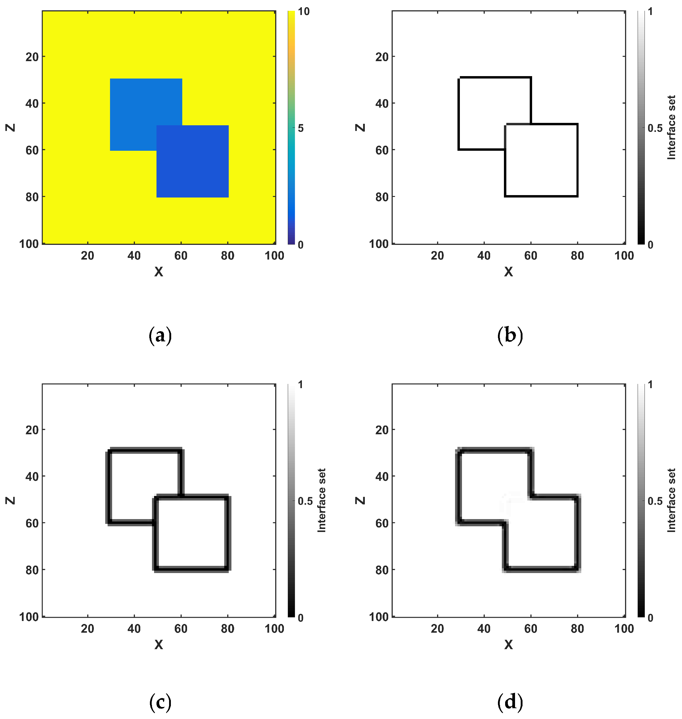
A simple model is shown in Figure 1a. The model consists of two square subunits. One square has an internal parameter value of 2, the other has a value of 1, and the background has a value of 10. The two squares partially overlap, and the numerical difference at their interface is smaller than the difference relative to the background parameters. To segment this model into subregions and interfaces, we use the shape-constrained regularization described in Equation (10). Figure 1b shows the interface results obtained under the optimal parameter setting. As β increases, the length of the interface set becomes smaller, i.e., the segmentation scale of the body inside the model becomes larger. And as ε increases, the recovered interfaces become more blurred. By choosing appropriate parameters, we can obtain a natural multi-scale strategy that improves inversion stability.
In general, if we aim to obtain more model details (small-scale information), we need to keep β and ε at small values; however, it should be noted that an excessively small ε will also affect the stability of segmentation.
Here, we present the strategies for the parameter value selection. The first concerns the α , which essentially serves as the weight coefficient for the L2-norm constraint term applied to the interior of segmented regions. Its selection can fully draw on the experience of Tikhonov regularization parameter tuning. When seismic amplitudes are normalized to the range of −1 to 1, the optimal alpha typically falls within the interval of 1 e 4 to 1 e 1 . Compared with L1-type regularization, the weight parameter of the L2-norm constraint is less sensitive, eliminating the need for extremely fine parameter tuning. For the Ambrosio–Tortorelli (AT) approximation, ε is generally required to be larger than the model grid interval to ensure numerical stability during the optimization process. However, in wave impedance inversion, the gradient differences are typically computed without considering the physical distance dimension, so the model grid interval can be treated as 1. Accordingly, it is recommended to set ε within the range of 1 to 10. Unless the inversion problem is severely ill-posed, an ε value greater than 10 will lead to excessively blurred boundaries, rendering the shape constraint ineffective. For the selection of the β parameter, its value is generally independent of the magnitude of the model and seismic data. It governs the penalty applied to the length of boundaries. The parameter sensitivity is highest within the range of 0.0001 to 0.001. When β exceeds 0.01, the sensitivity decreases, and further increases will only lead to excessive smoothing and blurring of structural features. Finally, it should be noted that for the selection of these parameters, the average energy of the first and second terms in Equation 10 should be kept as balanced as possible. An excessively large energy of the first term leads to over-smoothed inversion results, whereas an overly large energy of the second term gives rise to excessive spurious interfaces caused by noise.
The core advantage of the MS functional lies in its ability to permit discontinuities at these boundaries, whereas traditional Tikhonov regularization enforces global smoothness on the solution. Through the introduction above, we can conclude that incorporating this constraint into the inversion allows for a multi-scale characterization of geological boundaries, such as cavities and faults. Finally, by combining multi-trace seismic inversion with shape-constrained regularization, we obtain the objective function:
min f ( M , v ) = 1 2 D o b A M 2 2 + r s h a p e ( M , v ) .
For the minimization of Equation (12), optimization methods such as conjugate gradient, Newton and steepest descent methods can be used to optimize, thus solving for both M and v . The interfaces obtained by Equation (11) at a given iteration constitute the implicit shape representation for updating the impedance model in the next iteration.
The core physical advantage of this strategy is that it redefines inversion from a pixel-based grid optimization to a geo-body-based inversion. The shape of geo-bodies is mathematically represented by the interface set solved via the MS functional. Since the shape is not explicitly parameterized but implicitly defined by the boundaries, the proposed framework can be defined as an implicit shape-constrained inversion.
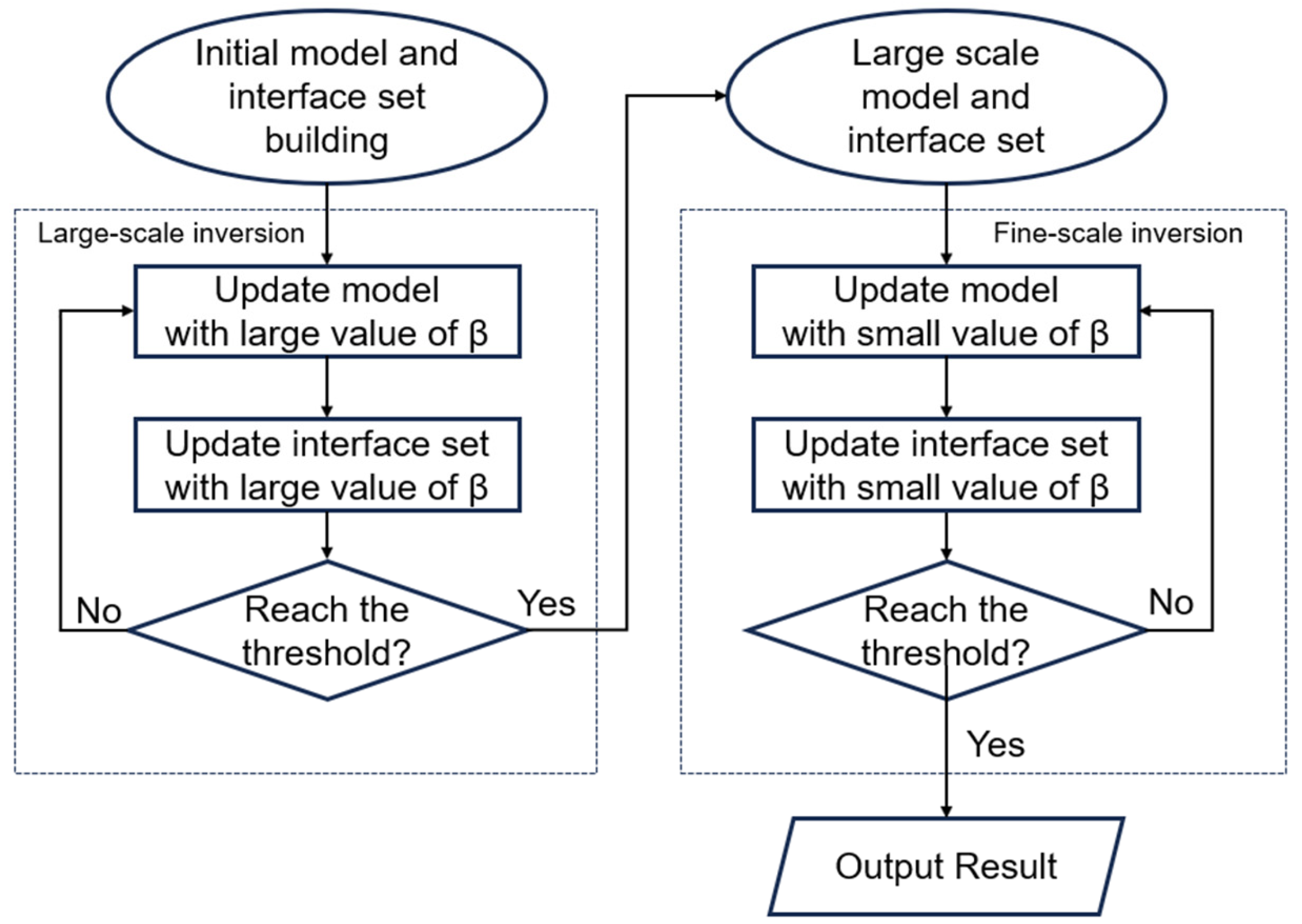
The workflow of the shape-constrained multi-trace seismic impedance inversion can be generalized as follows (Figure 2):
(1)
Estimation of seismic wavelet. In the synthetic recording case, we can simply use the wavelet used in the modeling of the observed data, such as the Ricker wavelet. However, in practical cases, we usually use a statistical wavelet in the target layer or estimate a wavelet by well-to-seismic calibration.
(2)
Initial model building. The prior information, such as logging and seismic interpretation, is used so that a smooth low-frequency model can be built.
(3)
Initialization of the interface set v . In general, we recommend that the interface set should all be initialized to 0, thus ensuring stable updates. However, if a reliable a priori model is available, the initial interfaces can also be set according to the geological understanding.
(4)
Solving the objective function. First, set a larger value of β and iteratively solve to obtain the large-scale inversion result, and then, based on the large-scale solution, we give a smaller value of β to obtain the fine solution. It should be noted that Equation (12) is biconvex, so alternating iterations are required to update the model M and interfaces v separately.

3. Synthetic Data Example

In this section, we apply the shape-constrained multi-trace inversion method (SCI) to a numerical model case to verify the effectiveness of the proposed method.
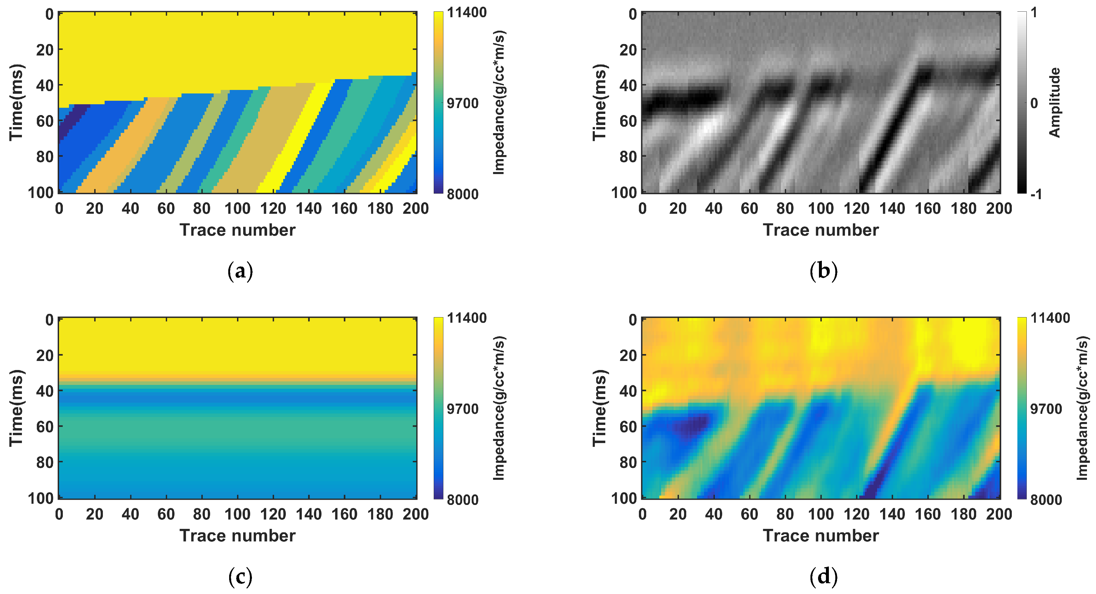
The numerical model (Figure 3a) is a segment extracted from a small portion of the Marmousi model and contains complex, steep structures, which can better demonstrate the advantages of the shape constraint [37]. The noise-free synthetic seismic data were calculated using Equation (5) in the previous section with a 25 Hz peak-frequency Ricker wavelet. We then add 10% Gaussian random noise to the noise-free data to obtain the observed data (Figure 3b). Both the model and synthetic data contain 201 traces, with 51 samples per trace and a sampling rate of 2 ms. We selected trace 121 of the true model as pseudo-log data, then smoothed and laterally extended it to construct the initial model (Figure 3c). For comparison with SC-I, the results of the conventional multi-trace inversion with prior model constraints (PCI) are shown in Figure 3d. The wavelet used for inversion is consistent with the forward wavelet, and the conjugate gradient method is employed with 10 iterations. It can be observed that the results obtained by the conventional PCI method exhibit strong smoothing effects, and the layered details of steep structures are significantly blurred, which is unfavorable for structural analysis and interpretation.
The second approach is the shape-constrained seismic inversion (SCI) proposed in this study, with which both impedance and interfaces are obtained simultaneously following the workflow shown in Figure 2. During the SCI, the wavelet and the number of iterations are kept consistent with those of PCI. Specifically, large-scale SCI is iterated five times, and small-scale SCI is iterated another five times, resulting in a total of ten iterations.
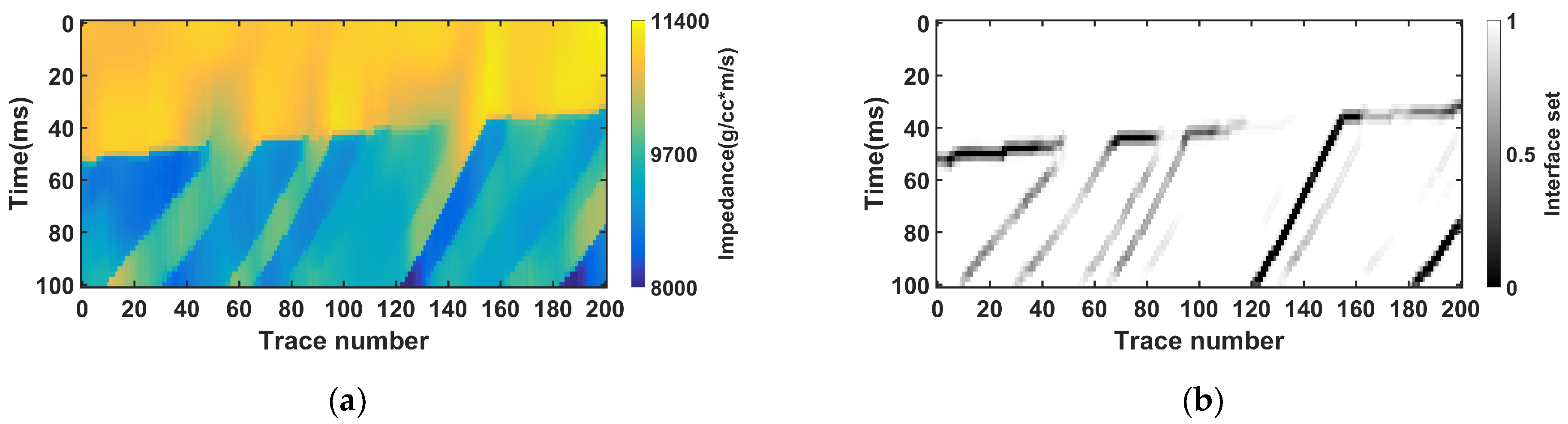
To ensure the stability of the inversion, we first perform the large-scale inversion, and the weighting factors of the shape-constrained regularization are set to α = 1 e 2 , β = 1 e 3 , ε = 2 (guided by the characteristic scales of the geological features). The impedance and interface set results from the large-scale inversion are shown in Figure 4.
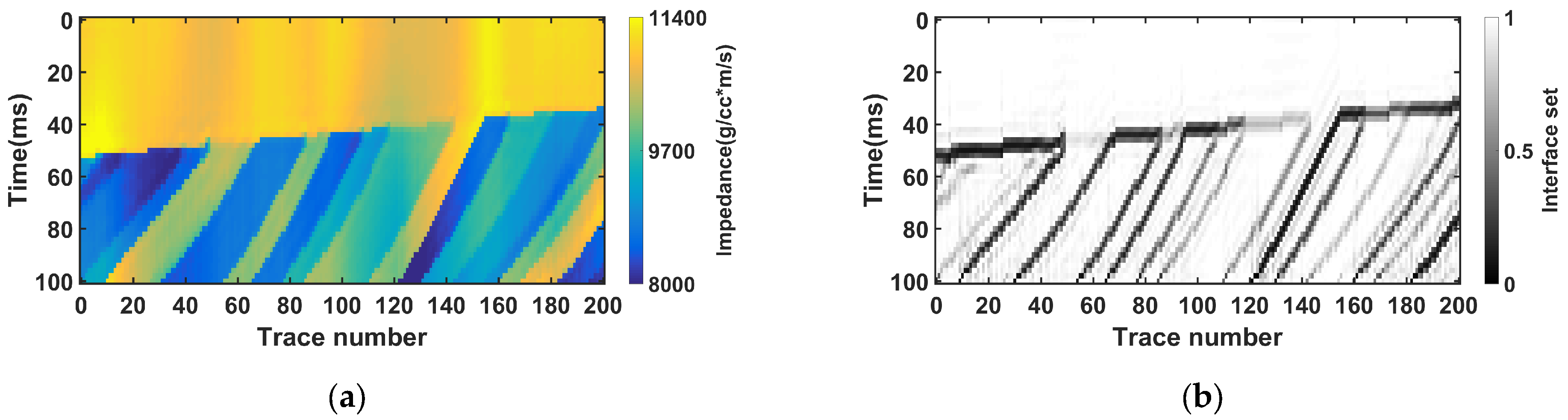
In Figure 4a, interfaces with large gradients are quite sharp. However, due to our strict constraint on the total interface length (controlled by the weighting factor β ), impedance interfaces with small gradients are smoothed. Figure 4b presents the inverted interface set, showing good agreement with the impedance model. In this process, the interface set acts not only as the target model but also as a constraint on the impedance update.
Although the large-scale inversion model is not the final output, this large-scale inversion step is often necessary. Directly performing small-scale inversion may lead to unstable inversion results and over-sharpened models, resulting in artifacts in the final output. We take the large-scale inversion results as the initial model and perform small-scale SCI, with the weighting factors set to α = 1 e 2 , β = 1 e 4 , ε = 2 . After five iterations, the results of the small-scale SCI are shown in Figure 5.
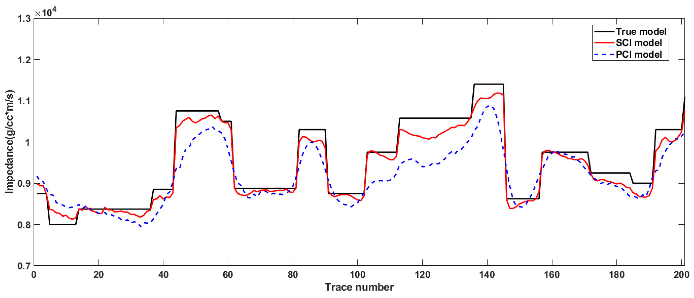
The inverted impedance shown in Figure 5a is structurally close to the true model, and the small-gradient details of the model are well characterized. This is because we have relaxed the penalty on the Euclidean metric of the length of interfaces, allowing more interface details to be recovered in the interface set compared with large-scale inversion, as illustrated in Figure 5b. Compared with the impedance model obtained by PIC (Figure 3d), the inversion result of SCI almost recovers the impedance interfaces of each steeply dipping structure, such as the thin layer on the far left at 60 ms. Similarly, the small-scale interface set is consistent with the impedance model, which can also help interpret the model structure. In addition, although the PCI method incorporates a Tikhonov regularization term, its inversion result still produces more artifacts in the high-impedance region above the model. This is because the prior information provided in this model test is unreliable, and the weight of the Tikhonov regularization term was not set sufficiently large. Increasing the weight would further over-smooth the model and make it closer to the erroneous structural information given in the initial model. Note that the PCI method employs a multi-trace inversion strategy in this experiment, and the results would be even poorer for the more common single-trace inversion. In contrast, the model-constrained regularization preserves the structural information from the inverted interface set while ensuring internal smoothness of the model.
To further quantitatively evaluate the influence of different inversion strategies on the recovery accuracy of acoustic impedance, a horizontal slice at 60 ms was selected from the model for detailed numerical comparison. In Figure 6, the red curve represents the shape-constrained inversion result proposed in this paper, the blue curve corresponds to the conventional prior-constrained inversion result, and the black curve denotes the true acoustic impedance as the reference benchmark. As can be observed from Figure 6, the SCI method not only exhibits advantages in structural information but also delivers higher numerical accuracy in the inverted impedance. We calculated the relative errors of the large-scale SCI, small-scale SCI, and PCI inversion results separately, and the corresponding results are presented in Table 1.
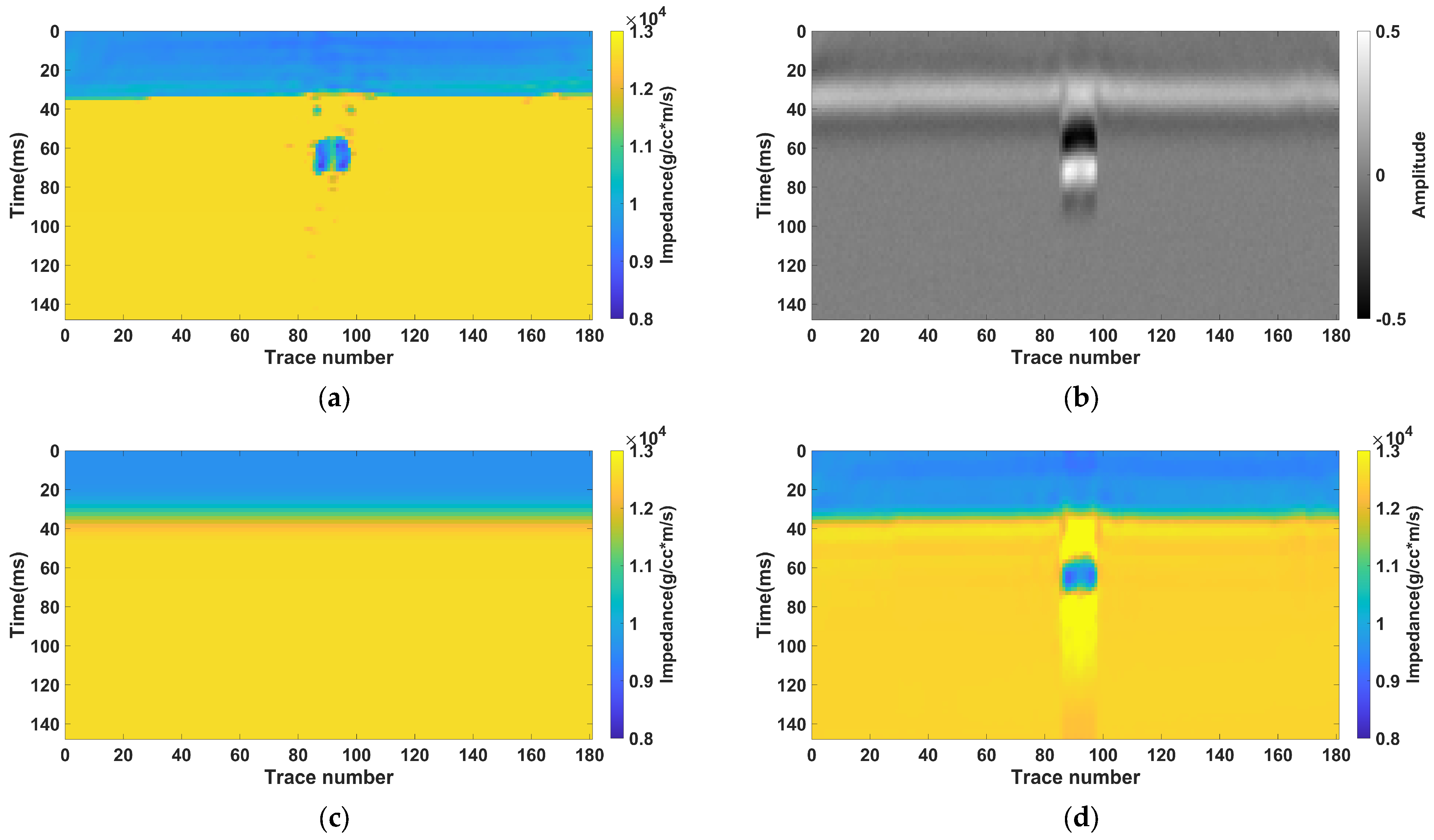
On this basis, we further test the proposed method on a simple numerical model of cavity reservoirs. In this test, we compare the cavity inversion performance of the SCI (Shape-Constrained Inversion) method with that of the Total Variation (TV) regularization inversion, which is widely used in edge-preserving seismic inversion. As shown in Figure 7, the panels display the true impedance model, the synthetic seismic data generated by forward modeling with a 25 Hz peak-frequency Ricker wavelet, the initial model for inversion, and the impedance model obtained by wave impedance inversion based on TV regularization, respectively. As observed in the TV-regularized inversion result, the internal details of the reservoir are excessively smoothed, with only large-scale stratigraphic interfaces preserved, and prominent band-like artifacts are introduced. TV regularization inherently favors piecewise-constant solutions, producing staircase-like boundaries aligned with horizontal or vertical directions. This makes it fundamentally incapable of accurately capturing the localized, irregular impedance contrasts characteristic of cavity reservoirs. Upon examining the zoomed-in local details, the internal edges of the cavity are noticeably “smeared out,” failing to recover sharp and well-defined boundary features. Furthermore, due to the strong gradients in seismic traces associated with fracture-cavity bodies, the high-impedance surrounding rock is also forced into artificial segmentation by the TV regularization. While TV regularization excels at handling large-scale, regular stratigraphic interfaces (e.g., horizontally layered media), it exhibits inherent limitations when applied to isolated, localized cavity reservoirs.
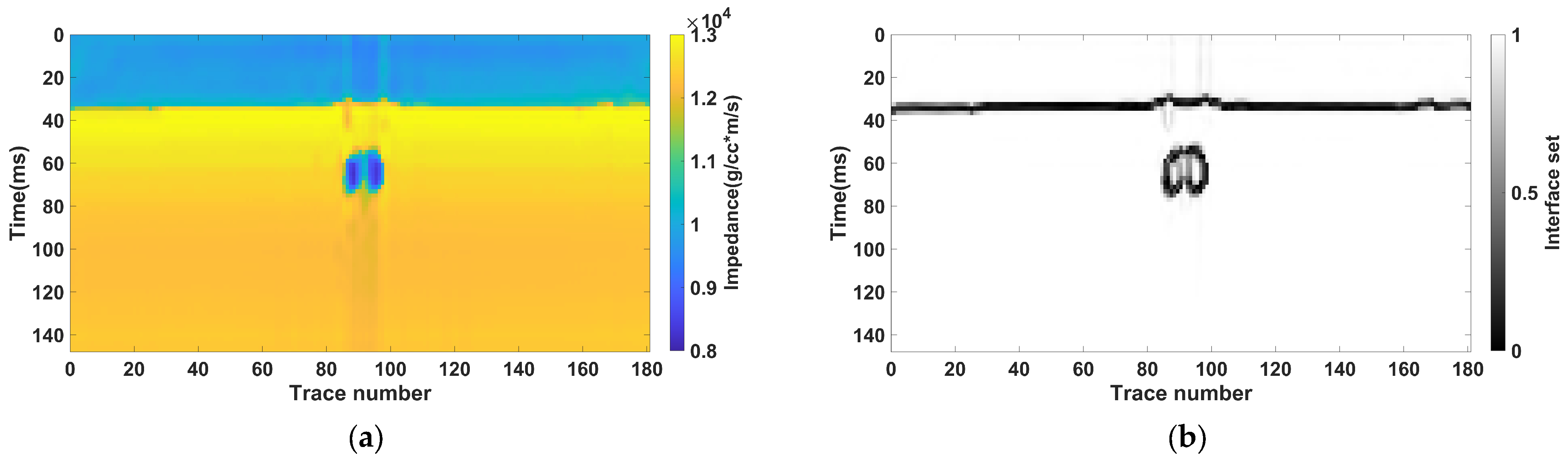
We also applied the proposed SCI method to the synthetic data of the cavity reservoir model, and the corresponding inversion results are presented in Figure 8. Compared with the TV-regularized inversion result, the SCI method yields a significantly improved impedance model for the cavity reservoir. The reservoir boundaries in the SCI result are sharp and well-defined, closely matching the true outline of the cavity, while the low-impedance features within the cavity are fully preserved, allowing clear identification of the reservoir’s internal architecture. This demonstrates that the SCI method effectively balances the preservation of large-scale stratigraphic interfaces and small-scale localized anomalies, achieving a favorable trade-off between edge retention and detail recovery.
The underlying difference lies in the regularization strategy. TV regularization imposes a uniform L1-norm penalty on the model gradient, which simultaneously suppresses variations in both the reservoir and the background. This leads to artificial segmentation of the high-impedance surrounding rock and the introduction of spurious artifacts. In contrast, the SCI method adopts a locally adaptive constraint mechanism: it specifically preserves and enhances impedance contrasts within the reservoir zone, while imposing no additional gradient penalties on the background high-impedance host rock. As a result, the background remains smooth and homogeneous without artificial artifacts.
Furthermore, while TV regularization inevitably and irreversibly attenuates high-frequency information associated with reservoir boundaries and internal structures during noise suppression, the SCI method leverages shape constraints to focus the inversion’s degrees of freedom on localized reservoir features. This allows the method to effectively recover high-frequency impedance variations within the low-impedance cavity, thereby retaining both the sharpness of reservoir boundaries and the fidelity of internal impedance distributions. These results comprehensively demonstrate the superior performance of the proposed SCI method when applied to discretely distributed cavity reservoirs. More importantly, the method effectively breaks through the inherent limitations of conventional edge-preserving inversion techniques in characterizing small-scale anomalous bodies.

4. Field Data Application

In the following, we apply shape-constrained inversion to real seismic data from a basin in northwestern China to characterize ultra-deep Ordovician carbonate cavity reservoirs. The target layer in this case is the Middle Ordovician marine carbonate strata with typical karst characteristics; the average depth of the target layer is as great as 6000 m. Affected by hydrothermal dissolution and multi-phase tectonic movements, spatially discrete cavity-type reservoirs are developed in the target interval [38,39].
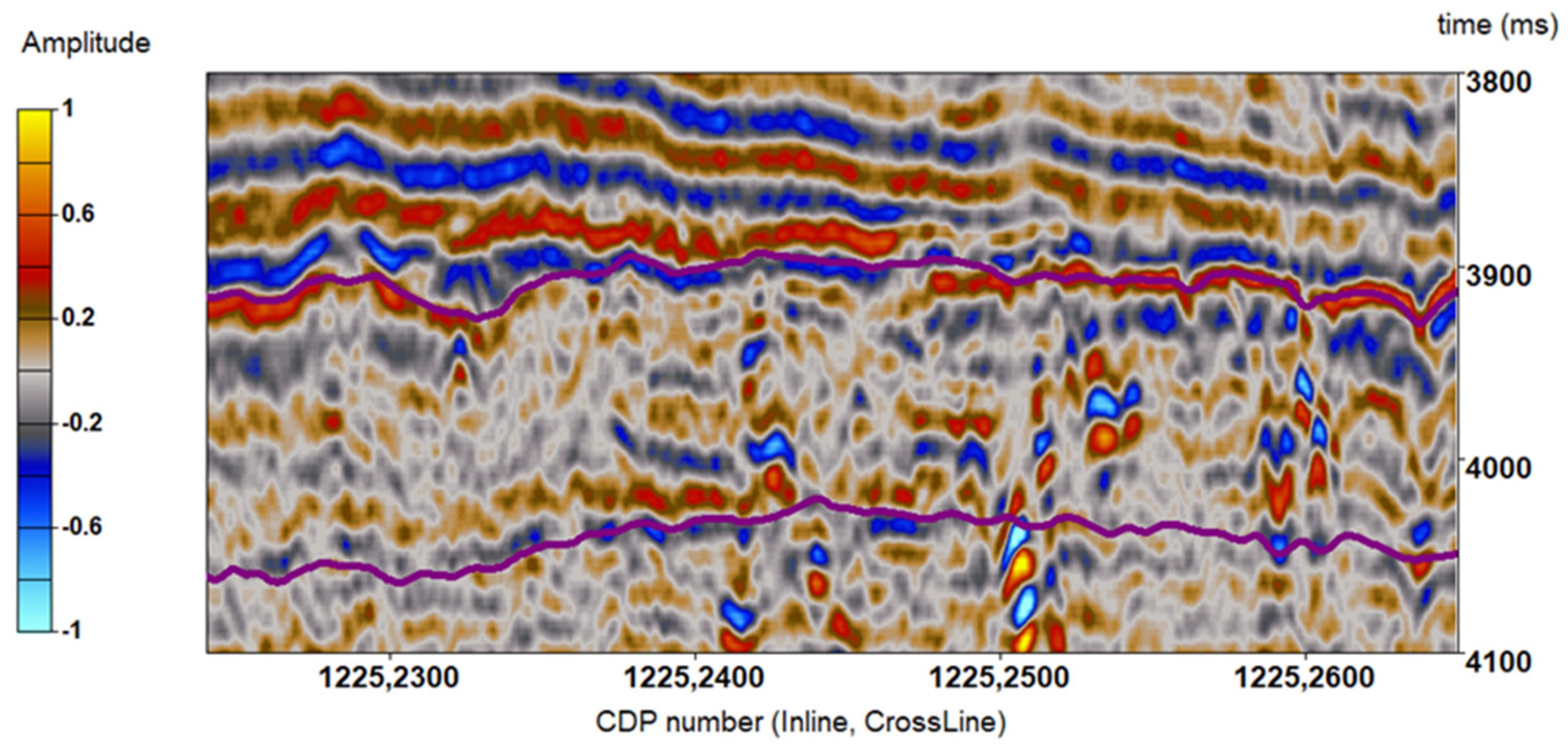
As shown in the local seismic profile of the target area (Figure 9), the seismic event axes are discontinuous and disordered, making it difficult to construct effective prior constraints. Furthermore, wells in the region experience drilling breaks or lost circulation upon drilling into the top of the cavities, resulting in sonic logs being available only in the upper part of the target interval, which poses challenges for constructing the initial model.
In this application, we simply extend the low-frequency logging impedance curve vertically and interpolate it along the top and bottom of the target formation to construct the initial model for inversion.
For comparison, we first calculate the relative impedance using sparse spike inversion, a common method in industrial applications. Its inversion result is shown in Figure 10. Sparse spike inversion fails to identify cavities and shows strong non-uniqueness. The curve labeled “AI” in the figure represents the acoustic impedance curve for Well A15 at this location; this well was not included in the initial model. It can be seen that the inversion results from sparse spike inversion show discrepancies from the locations of low-impedance anomalies in the logging curves. Furthermore, due to the effects of lateral smoothing and initial model constraints, the overall impedance variation is small, making it difficult to distinguish cavities from other geological features using thresholding.
Subsequently, we perform inversion on this seismic dataset using the shape-constrained strategy. The initial model and wavelet used in the inversion were consistent with those for sparse spike inversion.
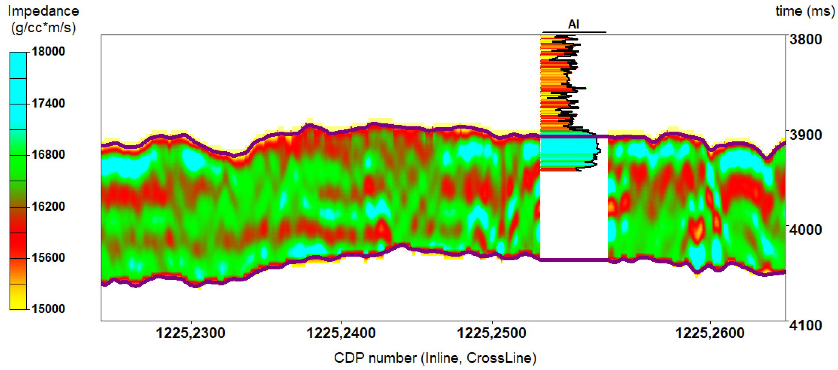
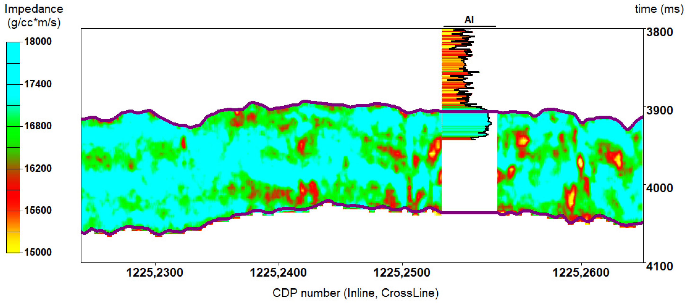
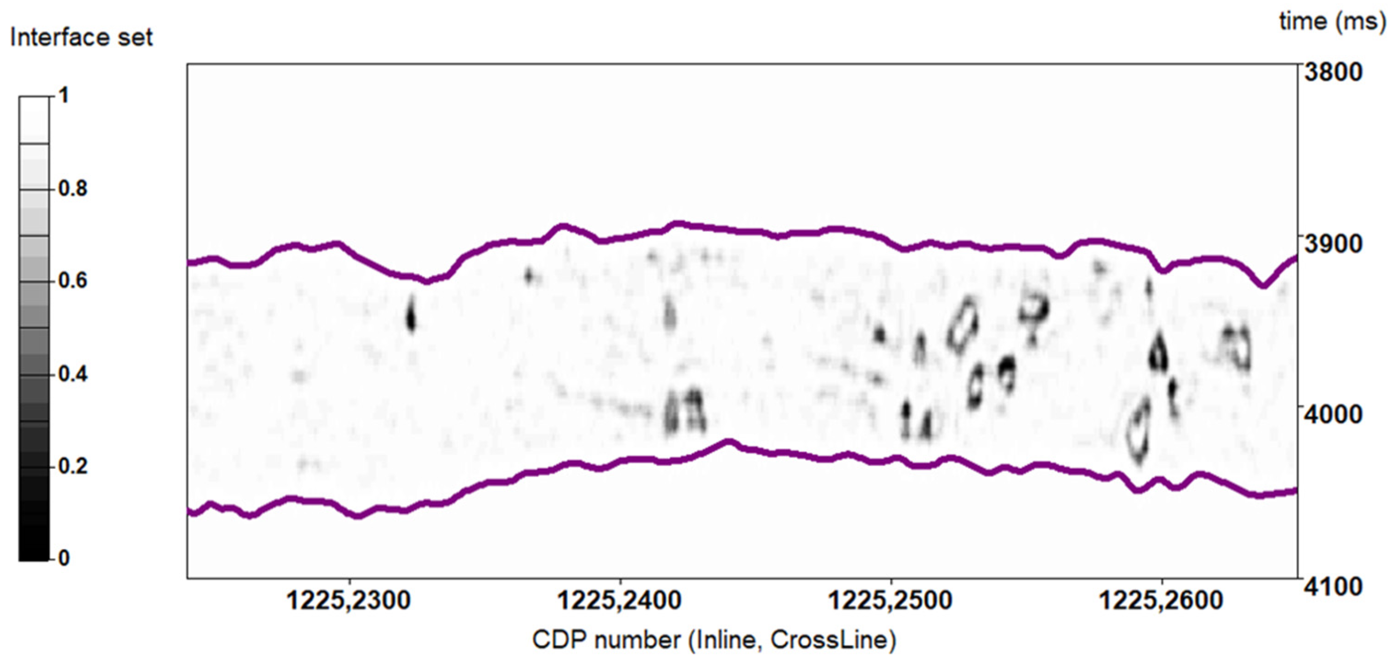
Figure 11 presents the impedance inversion result obtained by SCI, and Figure 12 shows the inversion result of the interface set. Compared with sparse spike inversion, the SCI result effectively highlights the low-impedance anomalies corresponding to cavity reservoirs and suppresses the extraneous layered artifacts in traditional inversion. The SCI result allows clear identification of the cavity geometry, which is consistent with the spatially discrete distribution of the strong-amplitude SBRs. Similarly, the inverted interface set can more intuitively delineate reservoir boundaries. Furthermore, verification using measured acoustic impedance curves from Well A15 shows that SCI achieves higher accuracy than conventional inversion methods. The locations of low-impedance anomalies identified by SCI inversion exhibit greater consistency with logging data.
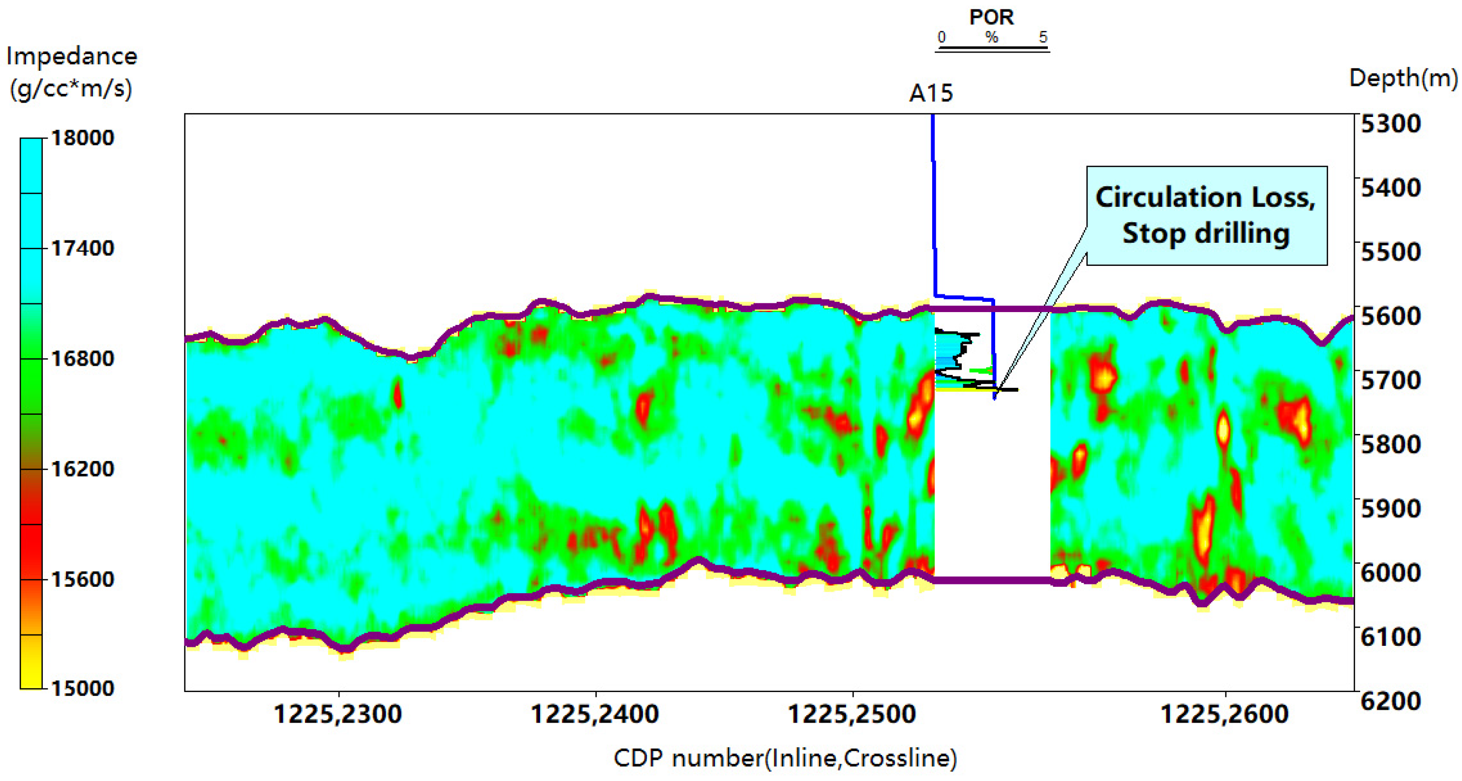
Figure 13 shows the inline1225 profile of the SCI impedance volume in the depth domain, where the blue line represents the projection of the well path of Well A15 on the profile. Drilling was suspended in Well A15 following a lost circulation incident at the bottom hole. In cavity reservoirs, the occurrence of lost circulation during drilling indicates that the wellbore has intersected a fracture-cavity system; therefore, such events serve as a critical indicator for reservoir identification [18]. As illustrated in Figure 11, the drilling suspension point (the location of the lost circulation event) along the well trajectory coincides exactly with the top of the cavity characterized by the SCI method.
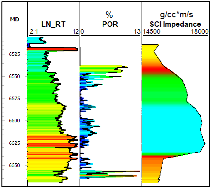
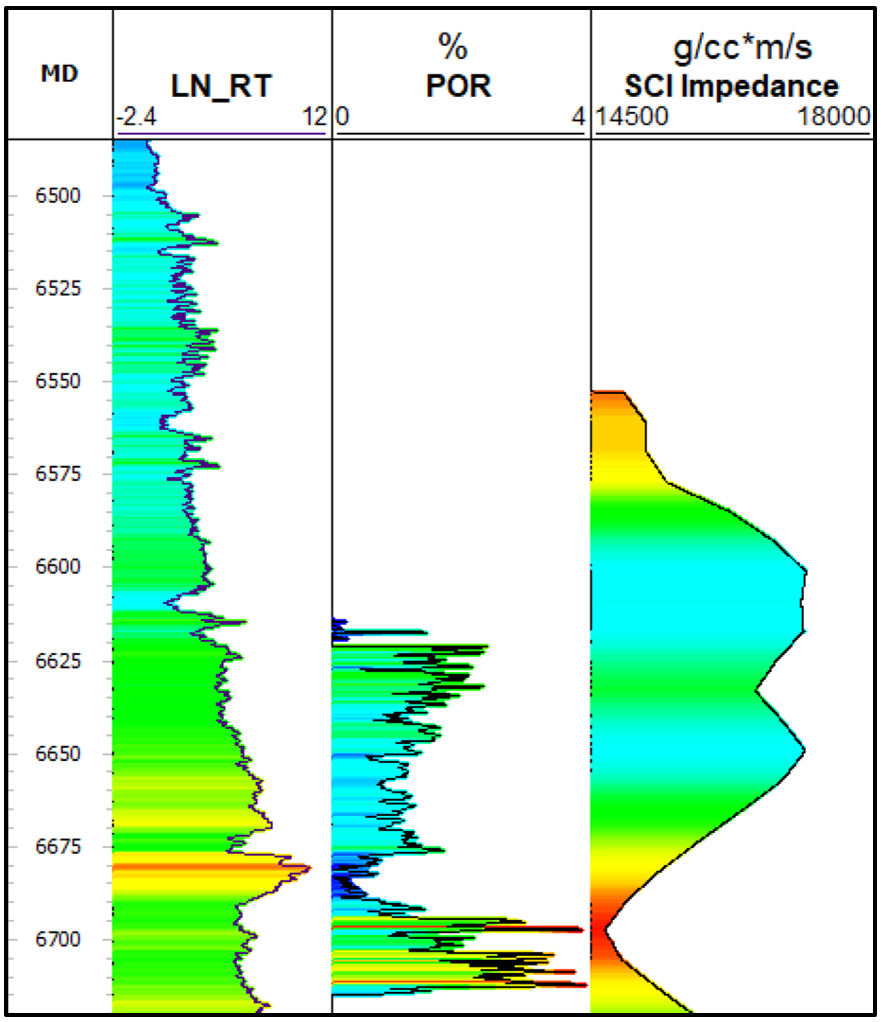
In addition, we extracted the SCI impedance along the trajectory of Well A15 for comparison with the logging curves (Figure 14). In Figure 14, MD represents the measured depth of the well, LN_RT denotes the natural logarithm of true resistivity, and POR stands for porosity. In ultra-deep carbonate cavity reservoirs, low acoustic impedance indicates widely developed fractures and caves, which usually correspond to high porosity because of increased void space within the formation. Meanwhile, such cavity zones are often saturated with hydrocarbons or filled with low-conductivity fluids, leading to high resistivity responses. Therefore, low impedance, high porosity, and high resistivity show a clear corresponding relationship, which can be used as a reliable criterion for identifying effective cavity reservoirs.
It can be observed that the low-impedance interval in the SCI impedance curve (corresponding to the top of the cavity characterized by SCI in Figure 13) coincides with the high-porosity interval from the measured porosity log. Meanwhile, LN_RT corresponds to high-resistivity zones, which are interpreted as effective reservoirs.
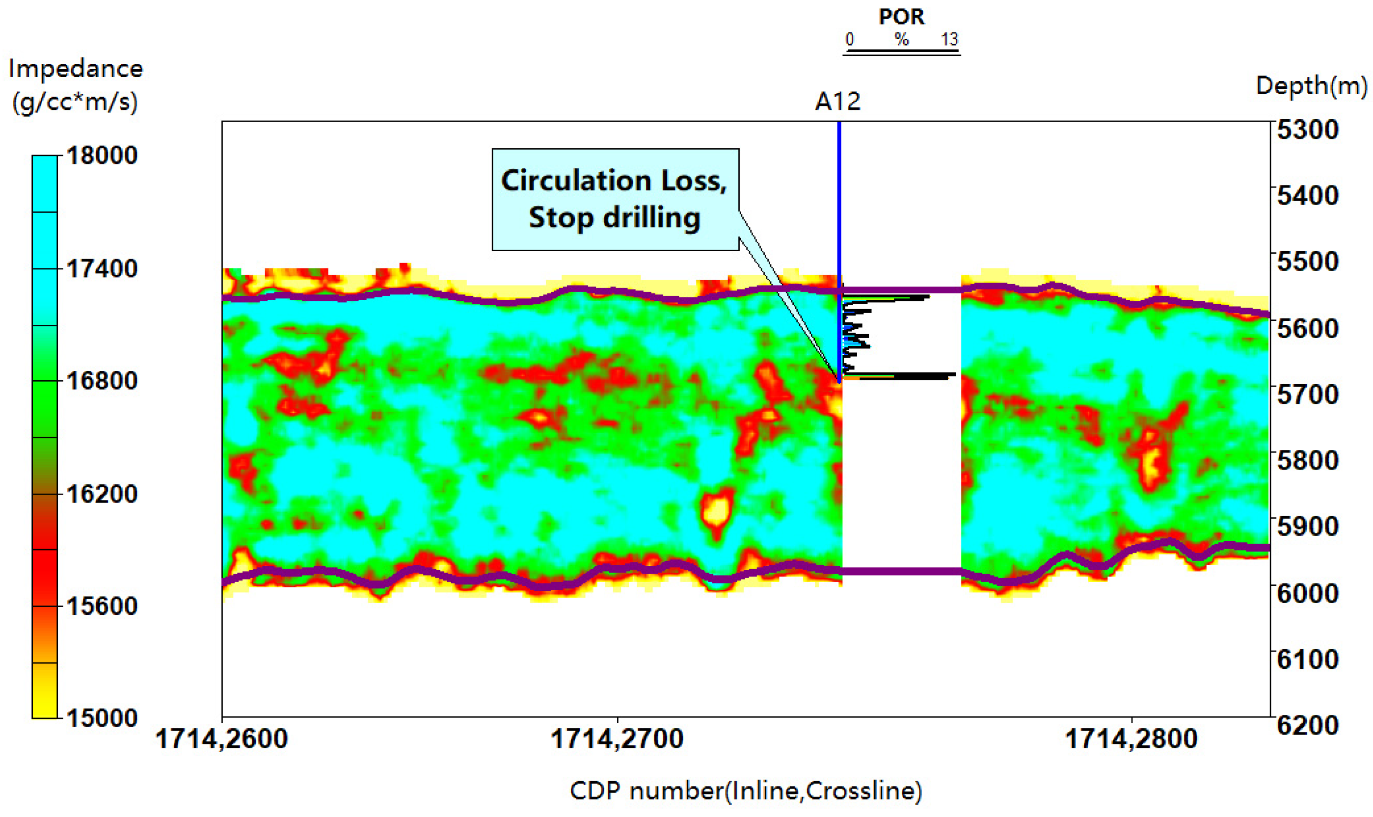
Similarly, we also present the depth-domain SCI impedance profile of inline 1714, as shown in Figure 15, where the blue line represents the well trajectory of Well A12. During the drilling operation of Well A12, a circulation loss and drilling break occurred at the end of the well trajectory, indicating that the bottom hole had connected with cavity reservoirs. The end of the well trajectory is precisely located at the top of the low-impedance anomaly in the profile, which is in agreement with our characterization results. Figure 16 shows the comparison between the SCI impedance extracted along the trajectory of Well A12 and the well-logging curves. The low-impedance interval from the inversion results corresponds well to the high-value interval of the measured porosity curve.

5. Discussion

Traditional pixel-based inversion suffers from structural inconsistency and non-uniqueness. In contrast, shape-constrained seismic inversion can well preserve sharp parameter jumps at geological interfaces, thereby highlighting anomalous geological bodies. This characteristic makes the shape-constrained inversion method particularly suitable for the characterization of spatially isolated cavity reservoirs. In the field data application in the Tarim Basin, the inversion results clearly reveal the spatial distribution pattern of karst reservoirs, which is in high agreement with the regional geological settings and well data. Compared with conventional impedance inversion, this method effectively reduces the uncertainty of reservoir interpretation.
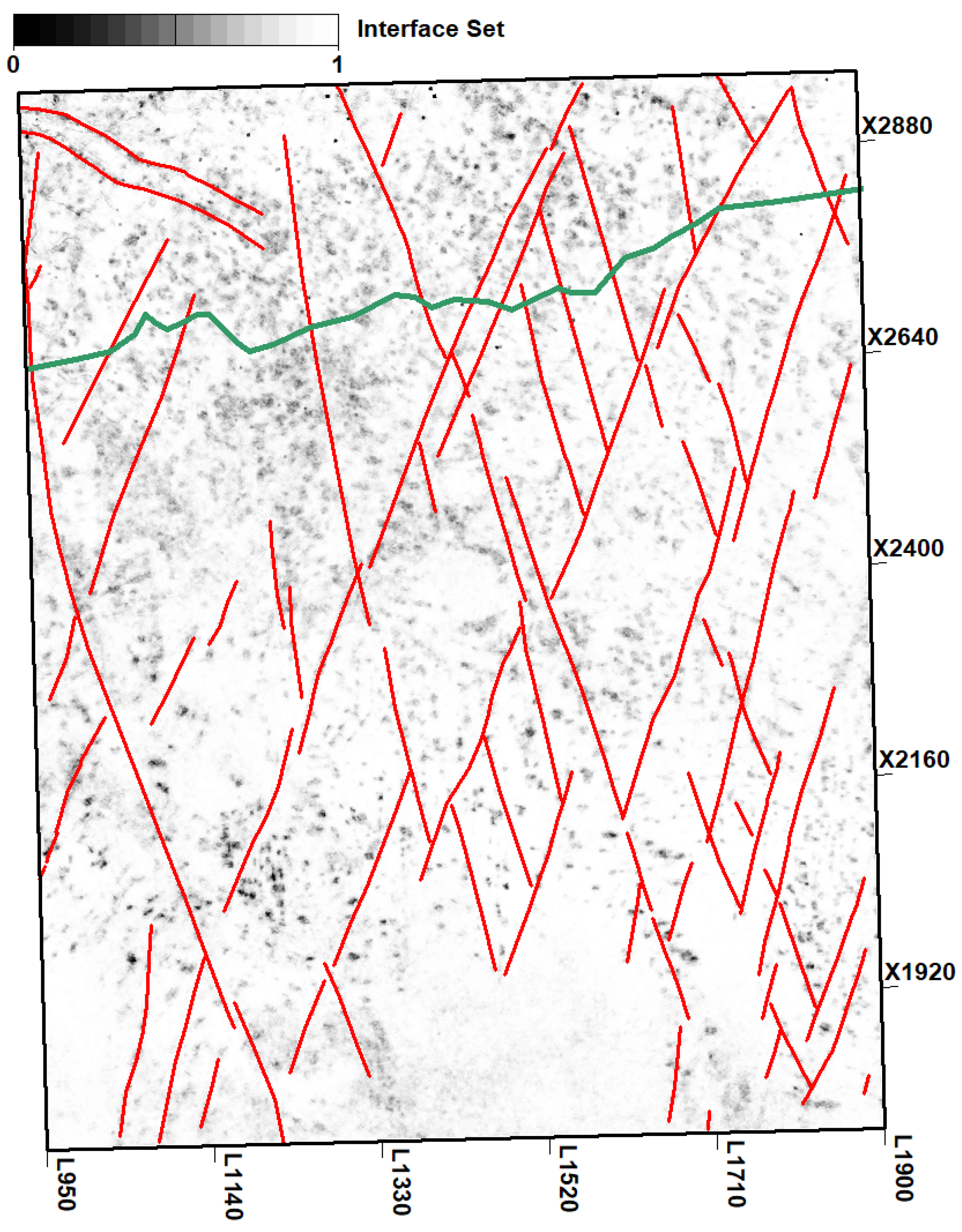
As one of the output products of shape-constrained inversion, the interface set can itself serve as a seismic attribute for reservoir characterization under reasonable weighting parameter settings, eliminating the need for threshold processing to delineate 3D reservoir bodies. For practical geological modeling, the inverted 3D interface sets can be adopted as facies-controlled constraints for modeling. Furthermore, the layered structural interfaces derived from seismic inversion can be reused as refined horizon boundaries to support stratigraphic subdivision and subsequent reservoir modeling. We completed the full 3D inversion for the work area described earlier, and Figure 17 shows the plan view of the target-layer interface set obtained from the shape-constrained inversion. It can be seen that the karst reservoir interfaces are widely distributed in the northern part of the work area, while in the southern part, they are mainly distributed in a banded pattern along strike-slip faults. The northern and southern parts of the work area belong to the buried-hill karst zone and the fault-controlled karst zone, respectively. This is because north of the pinch-out boundary of the overlying formation (green curve), the target layer has developed large-scale caves in the buried-hill karst zone [40,41]. It conforms to the prior geological knowledge of the region.
Although the proposed method has demonstrated its advantages and applicability, several practical aspects and methodological limitations deserve further discussion. The multi-trace inversion of 3D seismic data, as well as the iterative update and storage of interface sets, introduces additional computational and memory requirements. In the field data computation, the full dataset consists of 950 inlines, with each inline containing 1180 traces, and the vertical inversion dimension includes 400 sampling points. The calculation was carried out on a server equipped with 64 GB memory and 32 CPU cores, and the total computation time was 9 h. Notably, the shape-constrained inversion framework cannot be applied if the computation is restricted to a single-trace basis. In our practical application, we adopt the block-wise processing strategy to mitigate this issue, and we will continue to conduct research on improving computational efficiency in future work.
Second, the shape-constrained regularization term incorporates three weighting parameters, each of which controls the penalty weight for different model characteristics. The overall behavior is determined by their relative ratios rather than their absolute values. In future work, we will investigate adaptive parameter selection separately for large-scale and small-scale inversions.
Third, building on the existing research, we plan to integrate multi-source geological prior information—including sedimentary facies, fault systems, and karst paleogeomorphology—into the inversion framework to further enhance the geological rationality of the inversion results. Additionally, we will develop a depth-domain inversion framework to reduce errors associated with time–depth conversion. To address the challenges posed by depth-variable wavelets, we plan to introduce a depth-domain generalized S-transform, or a point spread function, to estimate the wavenumber information at each depth sampling point and construct a spatially variable wavelet [42]. This will enable depth-domain inversion, allowing the inversion results to be integrated more reliably into the 3D geological modeling workflow.

6. Conclusions

In this paper, we propose a method for characterizing cavity reservoirs based on shape-constrained seismic inversion and have conducted corresponding numerical experiments. On this basis, we apply the proposed method to real seismic field data.
The core innovation of this study lies in the introduction of the MS functional into multi-trace post-stack seismic impedance inversion. Implicit shape representation is achieved based on the MS functional framework. It forms only a narrow transition layer at true interfaces, avoiding the sacrifice of structural clarity of anomalous bodies for data misfit reduction in conventional inversion.
Numerical results confirm that shape-constrained inversion yields enhanced structural restoration compared to traditional techniques. Notably, even with limited prior information, it achieves significantly higher accuracy in impedance values and improved lateral resolution. This is because the inversion framework implicitly promotes piecewise constant regions, drastically reducing the degrees of freedom in the optimization process.
Case studies in the actual field demonstrate that the proposed method offers significant improvements in characterizing cavity-type reservoirs compared to traditional approaches. By implicitly identifying cavities as piecewise constant regions rather than isolated grid cells, we drastically reduce non-physical degrees of freedom, preserve sharp impedance contrasts at true cavity boundaries, and avoid over-smoothing low-impedance reservoir anomalies. This makes the method uniquely suited for characterizing discrete, sharp-boundary carbonate cavity reservoirs. Through correlation with drilling and logging data, we confirm that the interpreted cavity-type reservoirs in wells are consistent with our results, thereby validating the reliability and authenticity of the cavity characterization.
These validation results demonstrate that the proposed method can effectively characterize the structural morphology of subsurface anomalous bodies, thereby providing valuable support for hydrocarbon exploration in highly heterogeneous reservoirs such as carbonates.

Author Contributions

Conceptualization, K.L. and X.H.; methodology, K.L. and X.C.; software, D.Z.; validation, L.N.; writing—original draft preparation, K.L.; writing—review and editing, X.H. and X.C.; visualization, D.Z. and L.N.; funding acquisition, K.L. All authors have read and agreed to the published version of the manuscript.

Funding

This research was funded by the National Natural Science Foundation of China under Grant U23B6010.

Institutional Review Board Statement

Not applicable.

Informed Consent Statement

Not applicable.

Data Availability Statement

The raw data supporting the conclusions of this article will be made available by the authors on request.

Conflicts of Interest

Authors Kai Li, Dan Zhou and Liping Niu were employed by the SINOPEC Geophysical Research Institute Co., Ltd. The remaining authors declare that the research was conducted in the absence of any commercial or financial relationships that could be construed as a potential conflict of interest.

References

  1. Wu, G.; Gao, L.; Zhang, Y.; Ning, C.; Xie, E. Fracture attributes in reservoir-scale carbonate fault damage zones and implications for damage zone width and growth in the deep subsurface. J. Struct. Geol. 2019, 118, 181–193. [Google Scholar] [CrossRef] [Scilit]
  2. Liu, B.; Yang, F.; Zhang, G.; Zhao, L. Pre-stack fracture prediction in an unconventional carbonate reservoir: A case study of the M oilfield in Tarim Basin, NW China. Energies 2024, 17, 2061. [Google Scholar] [CrossRef] [Scilit]
  3. Adam, A.; Swennen, R.; Abdulghani, W.; Abdlmutalib, A.; Hariri, M.; Abdulraheem, A. Reservoir heterogeneity and quality of Khuff carbonates in outcrops of central Saudi Arabia. Mar. Pet. Geol. 2018, 89, 721–751. [Google Scholar] [CrossRef] [Scilit]
  4. Zhang, J.; Ma, P.; Liu, Y.; Dongming, L.; Li, X.; Xin, L.; Leli, W. Control modes of multitype strike-slip fault systems on fractured-vuggy carbonate reservoir development. In SEG Technical Program Expanded Abstracts 2016, Dallas, TX, USA, 16–21 October 2016; Society of Exploration Geophysicists: Houston, TX, USA, 2016; pp. 1813–1817. [Google Scholar] [CrossRef] [Scilit]
  5. Deng, Z.; Zhou, D.; Dong, H.; Huang, X.; Wei, S.; Kang, Z. Deep learning for predicting porosity in ultra-deep fractured vuggy reservoirs from the Shunbei oilfield in Tarim Basin, China. Sci. Rep. 2024, 14, 29605. [Google Scholar] [CrossRef] [Scilit] [PubMed]
  6. Gong, W.; Wen, X.; Zhou, D. Characteristics and seismic identification mode of ultra-deep carbonate fault-controlled reservoir in Northwest China. Energies 2022, 15, 8598. [Google Scholar] [CrossRef] [Scilit]
  7. Wang, Y.; Xie, P.; Zhang, H.; Liu, Y.; Yang, A. Fracture-vuggy carbonate reservoir characterization based on multiple geological information fusion. Front. Earth Sci. 2024, 11, 1345028. [Google Scholar] [CrossRef] [Scilit]
  8. Qi, L. Structural characteristics and storage control function of the Shun I fault zone in the Shunbei region, Tarim Basin. J. Pet. Sci. Eng. 2021, 203, 108653. [Google Scholar] [CrossRef] [Scilit]
  9. Han, S.; Wang, S.; Lan, H.T.; Wang, Z. Application of Multi-attribute Clustering Technology to Description of Fault-Controlled Fracture-Cavity Reservoirs in Changxing Formation, Longgang Area. In Proceedings of the International Field Exploration and Development Conference 2023 (IFEDC 2023); Lin, J., Ed.; Springer: Singapore, 2024; pp. 409–422. [Google Scholar] [CrossRef] [Scilit]
  10. Zhen, W.; Huan, W.; Guangxiao, D.; Wei, D.; Xin, W. Fault-karst characterization technology in the Tahe Oilfield, China. Geophys. Prospect. Pet. 2019, 58, 149–154. [Google Scholar] [CrossRef]
  11. Wang, L.; Yang, R.; Li, D.; Meng, L.; Xiao, Z. Seismic attributes for characterization and prediction of carbonate faulted karst reservoirs in the Tarim Basin, China. Interpretation 2021, 9, T611–T622. [Google Scholar] [CrossRef] [Scilit]
  12. Li, Z.; Li, H.; Liu, J.; Deng, G.; Gu, H.; Yan, Z. 3D seismic intelligent prediction of fault-controlled fractured-vuggy reservoirs in carbonate reservoirs based on a deep learning method. J. Geophys. Eng. 2024, 21, 345–358. [Google Scholar] [CrossRef] [Scilit]
  13. Cao, D.; Yin, X.; Zhang, F. Impedance inversion method constrained with crosswell seismic data. In Beijing International Geophysical Conference and Exposition 2009, Beijing, China, 13–17 April 2009; Society of Exploration Geophysicists: Houston, TX, USA, 2009; Volume 10, p. 261. [Google Scholar] [CrossRef] [Scilit]
  14. Ye, D.; He, L.; Ren, J.; Wang, X.; Bian, L. Application of Seismic Inversion Technology Based on Complicated Structure Modeling. In International Geophysical Conference 2018, Beijing, China, 24–27 April 2018; Society of Exploration Geophysicists & Chinese Petroleum Society: Beijing, China, 2018; pp. 1095–1099. [Google Scholar] [CrossRef] [Scilit]
  15. Hameed, M.; Al-Qallaf, H.; Razak, M.H.A. Geostatistical Inversion-Carbonate Case Studies from Kuwait. In 75th EAGE Conference & Exhibition Incorporating SPE EUROPEC 2013, London, UK, 10–13 June 2013; European Association of Geoscientists & Engineers: Houten, The Netherlands, 2013; p. cp-348. [Google Scholar] [CrossRef] [Scilit]
  16. Liu, H.; Ren, L.; Hu, Z. Pressure curve characteristics for wells drilled in cave of fracture-cavity carbonate reservoirs. Lithol. Reserv. 2012, 24, 124–128. [Google Scholar] [CrossRef]
  17. Lan, X.; Lü, X.; Zhu, Y.; Yu, H. The geometry and origin of strike-slip faults cutting the Tazhong low rise megaanticline (central uplift, Tarim Basin, China) and their control on hydrocarbon distribution in carbonate reservoirs. J. Nat. Gas Sci. Eng. 2015, 22, 633–645. [Google Scholar] [CrossRef] [Scilit]
  18. Li, X.; Li, J.; Feng, X.; Dan, G.; Zhang, G.; Zhang, L.; Zhao, W. Heterogeneous reservoir prediction of ultra-deep strike-slip fault-damaged zone constrained with local seismic anomaly data. Earth Sci. Inform. 2022, 15, 1427–1441. [Google Scholar] [CrossRef] [Scilit]
  19. Yonglei, L.; Zujun, W.; Zhenzhou, L.; Xiangwen, L. The application of phase-controlled inversion in prediction of deeply buried marine reef-bank reservoirs in the central Tarim Basin. In SPG/SEG 2016 International Geophysical Conference, Beijing, China, 20–22 April 2016; Society of Exploration Geophysicists & Society of Petroleum Geophysicists: Beijing, China, 2016; pp. 734–737. [Google Scholar] [CrossRef] [Scilit]
  20. Wang, C.; Shi, X.; Jing, B.; Xie, E. Characterization of carbonate reservoirs based on geostatistics inversion with lithofacies model: A case study in Tarim Oilfield of China. In SEG Technical Program Expanded Abstracts 2017, Houston, TX, USA, 24–29 September 2017; Society of Exploration Geophysicists: Houston, TX, USA, 2017; pp. 3007–3011. [Google Scholar] [CrossRef] [Scilit]
  21. Li, K.; Huang, X.; Wo, Y.; Cao, W.; Hu, Y.; Tang, J.; Xiao, W. A characterization method for cavity Karst reservoir using local full-waveform inversion in frequency domain. IEEE Geosci. Remote Sens. Lett. 2023, 20, 1–5. [Google Scholar] [CrossRef] [Scilit]
  22. Ge, Q.; Cao, H.; Yang, Z.F.; Li, X.M.; Yan, X.F.; Zhang, X.; Wang, Y.Q.; Lu, W.K. High-resolution seismic impedance inversion integrating the closed-loop convolutional neural network and geostatistics: An application to the thin interbedded reservoir. J. Geophys. Eng. 2022, 19, 550–561. [Google Scholar] [CrossRef] [Scilit]
  23. Song, C.; Lu, W.; Ye, S.; Yao, W.; Zhang, X. Multimodal geophysics-informed neural network for joint inversion of seismic electromagnetic and well-logging. IEEE Trans. Geosci. Remote Sens. 2026, 64, 5906613. [Google Scholar] [CrossRef] [Scilit]
  24. Gholami, A. Nonlinear multichannel impedance inversion by total-variation regularization. Geophysics 2015, 80, R217–R224. [Google Scholar] [CrossRef] [Scilit]
  25. Gholami, A. A fast automatic multichannel blind seismic inversion for high-resolution impedance recovery. Geophysics 2016, 81, V357–V364. [Google Scholar] [CrossRef] [Scilit]
  26. Dai, R.; Zhang, F.; Yin, C.; Hu, Y. Multi-trace post-stack seismic data sparse inversion with nuclear norm constraint. Acta Geophys. 2021, 69, 53–64. [Google Scholar] [CrossRef] [Scilit]
  27. Cheng, L.; Wang, S.; Li, S.; Ji, Y. Multi-trace nonstationary sparse inversion with structural constraints. Acta Geophys. 2020, 68, 675–685. [Google Scholar] [CrossRef] [Scilit]
  28. Guo, K.; Li, J.; Chen, X.; Yang, W.; Zhu, G.; Liu, X. Multi-trace acoustic impedance inversion with multiplicative regularization. J. Appl. Geophys. 2021, 186, 104263. [Google Scholar] [CrossRef] [Scilit]
  29. Yun, Z.; Zhijiang, K. Key Technologies for Oil and Gas Development from Deep Carbonate Fractured-Vuggy Reservoirs. J. Immunol. Res. Rep. 2023, 3, 1–11. [Google Scholar] [CrossRef] [Scilit]
  30. Mumford, D.; Shah, J. Optimal approximations by piecewise smooth functions and associated variational problems. Commun. Pure Appl. Math. 1989, 42, 577–685. [Google Scholar] [CrossRef] [Scilit]
  31. Verschuur, D.J.; Berkhout, A.J. Estimation of multiple scattering by iterative inversion; Part II, Practical aspects and examples. Geophysics 1997, 62, 1596–1611. [Google Scholar] [CrossRef] [Scilit]
  32. Margrave, G.F.; Lamoureux, M.P.; Henley, D.C. Gabor deconvolution: Estimating reflectivity by nonstationary deconvolution of seismic data. Geophysics 2011, 76, W15–W30. [Google Scholar] [CrossRef] [Scilit]
  33. Cooke, D.A.; Schneider, W.A. Generalized linear inversion of reflection seismic data. Geophysics 1983, 48, 665–676. [Google Scholar] [CrossRef] [Scilit]
  34. Tikhonov, A.N.; Goncharsky, A.V.; Stepanov, V.V.; Yagola, A.G. Numerical Methods for the Solution of Ill-Posed Problems; Springer: Dordrecht, The Netherlands, 1995; pp. 65–79. [Google Scholar]
  35. Ambrosio, L.; Tortorelli, V.M. Approximation of functional depending on jumps by elliptic functional via Γ-convergence. Commun. Pure Appl. Math. 1990, 43, 999–1036. [Google Scholar] [CrossRef] [Scilit]
  36. Wang, C.; Liu, Z.; Liu, L. Feature-preserving Mumford–Shah mesh processing via nonsmooth nonconvex regularization. Comput. Graph. 2022, 106, 222–236. [Google Scholar] [CrossRef] [Scilit]
  37. Martin, G.S.; Wiley, R.; Marfurt, K.J. Marmousi2: An elastic upgrade for Marmousi. Lead. Edge 2006, 25, 156–166. [Google Scholar] [CrossRef] [Scilit]
  38. Li, X.; Li, J.; Li, L.; Wan, Z.; Liu, Y.; Ma, P.; Zhang, M. Seismic wave field anomaly identification of ultra-deep heterogeneous fractured-vuggy reservoirs: A case study in Tarim Basin, China. Appl. Sci. 2021, 11, 11802. [Google Scholar] [CrossRef] [Scilit]
  39. Gao, Z.; Liu, Z.; Gao, S.; Ding, Q.; Wu, S.; Liu, S. Characteristics and genetic models of Lower Ordovician carbonate reservoirs in southwest Tarim Basin, NW China. J. Pet. Sci. Eng. 2016, 144, 99–112. [Google Scholar] [CrossRef] [Scilit]
  40. Tian, F.; Luo, X.; Zhang, W. Integrated geological-geophysical characterizations of deeply buried fractured-vuggy carbonate reservoirs in Ordovician strata, Tarim Basin. Mar. Pet. Geol. 2019, 99, 292–309. [Google Scholar] [CrossRef] [Scilit]
  41. Li, J.; Zhang, Z.; Zhu, G.; Li, T.; Zhao, K.; Chi, L.; Yan, H. The origin and accumulation of ultra-deep oil in Halahatang area, northern Tarim Basin. J. Pet. Sci. Eng. 2020, 195, 107898. [Google Scholar] [CrossRef] [Scilit]
  42. Li, K.; Niu, L.; Zhou, D.; Meng, S. Depth-Domain Direct Inversion Based on Depth-Variant Wavelet Under Geo-Structure Constraints. In Proceedings of the 86th EAGE Annual Conference & Exhibition, Toulouse, France, 2–5 June 2025. [Google Scholar] [CrossRef] [Scilit]
Figure 1. The simple numerical model and the interface sets obtained with different weighting parameters: (a) the simple numerical model; (b) the interface set v obtained with small values for β and ε ; (c) the interface set v obtained with a small value for β and a larger value for ε ; and (d) the interface set v obtained with large values for β and ε .
Eng 07 00222 g001
Figure 2. Workflow of the shape-constrained seismic inversion.
Eng 07 00222 g002
Figure 3. The numerical model and its conventional prior-constrained inversion result: (a) the numerical impedance model; (b) the synthetic record with 10% Gaussian random noise; (c) the initial model obtained by lateral extrapolation of pseudo-well data; amd (d) the impedance model obtained by the conventional prior-constrained inversion.
Eng 07 00222 g003
Figure 4. The impedance and interface set results obtained by large-scale SCI: (a) the impedance model obtained by large-scale shape-constrained seismic inversion and (b) the interface set obtained by large-scale shape-constrained seismic inversion.
Eng 07 00222 g004
Figure 5. The impedance and interface set results obtained by small-scale SCI: (a) the impedance model obtained by small-scale shape-constrained seismic inversion and (b) the interface set obtained by small-scale shape-constrained seismic inversion.
Eng 07 00222 g005
Figure 6. Comparison of time slices at 60 ms between the true impedance and inversion results obtained using different inversion strategies. The red curve denotes the inversion result of the proposed shape-constrained inversion strategy, the blue curve represents the result obtained by the conventional prior-constrained inversion strategy, and the black curve indicates the true acoustic impedance as a reference.
Eng 07 00222 g006
Figure 7. The cavity numerical model and its inversion result with TV regularization: (a) the numerical impedance model; (b) the synthetic record with 10% Gaussian random noise; (c) the initial model of the inversion; and (d) the impedance model obtained by the TV regularization inversion.
Eng 07 00222 g007
Figure 8. The impedance and interface set results of the cavity numerical model obtained by SCI: (a) the impedance model and (b) the interface set.
Eng 07 00222 g008
Figure 9. The time-domain seismic profile of the target interval from the study area. The purple curves represent the top and bottom of the target interval.
Eng 07 00222 g009
Figure 10. The time-domain impedance profile of the target interval obtained by the single-trace sparse spike inversion method. The curve labeled “AI” is the acoustic impedance logging curve for Well A15, and its values are filled with the same color legend as the impedance profile.
Eng 07 00222 g010
Figure 11. The time-domain impedance profile of the target interval obtained by the shape-constrained inversion method. The curve labeled “AI” is the acoustic impedance logging curve for Well A15, and its values are filled with the same color legend as the impedance profile.
Eng 07 00222 g011
Figure 12. The time-domain impedance profile of the target interval obtained by the shape-constrained inversion method.
Eng 07 00222 g012
Figure 13. The inline1225 SCI impedance profile converted to the depth domain through time-depth conversion. The blue line denotes the projection of Well A15’s well trajectory onto the profile, where drilling was terminated due to a circulation loss event at the end of the trajectory. The curve along the well trajectory is the measured porosity log.
Eng 07 00222 g013
Figure 14. Comparison of the SCI impedance curve and well-logging curves along the Well A15 trajectory. MD denotes measured depth, LN_RT denotes the natural logarithm of true resistivity, POR denotes measured porosity, and SCI impedance represents the inversion result extracted along the well trajectory.
Eng 07 00222 g014
Figure 15. The inline1714 SCI impedance profile converted to the depth domain through time-depth conversion. The blue line denotes the projection of Well A12’s well trajectory onto the profile, where drilling was terminated due to a circulation loss event at the end of the trajectory. The curve along the well trajectory is the measured porosity log.
Eng 07 00222 g015
Figure 16. Comparison of the SCI impedance curve and well-logging curves along the Well A12 trajectory. MD denotes measured depth, LN_RT denotes the natural logarithm of true resistivity, POR denotes measured porosity, and SCI impedance represents the inversion result extracted along the well trajectory.
Eng 07 00222 g016
Figure 17. Slice of the interface set along the target horizon over the full survey. Among them, the red lines represent the strike-slip fault system of the target layer, and the green curves denote the pinch-out lines of the overlying strata.
Eng 07 00222 g017
Table 1. Comparison of the relative errors of the impedance results using different inversion methods.
Inversion MethodsRelative Errors
Large-scale SCI0.1030
Small-scale SCI0.0233
PCI0.0791
The small-scale SCI result is obtained by performing five additional iterations based on the large-scale SCI result.
Disclaimer/Publisher’s Note: The statements, opinions and data contained in all publications are solely those of the individual author(s) and contributor(s) and not of MDPI and/or the editor(s). MDPI and/or the editor(s) disclaim responsibility for any injury to people or property resulting from any ideas, methods, instructions or products referred to in the content.