Sensitivity Analysis of UH Model Parameters for Granite Residual Soils in the Fujian–Guangdong Region

Abstract

This study collected 155 sets of test data for granite residual soils from the Fujian–Guangdong region and applied the chi-square test to analyze the distributions of eight common physical and mechanical parameters. Drained triaxial tests were then simulated using the Unified Hardening (UH) model, and a Sobol global sensitivity analysis of model parameters was conducted based on the distributions of soil properties. The results show that natural density and cohesion approximately follow Weibull distributions; void ratio, liquid limit and plastic limit follow lognormal distributions; water content and internal friction angle follow normal distributions; and plasticity index follows a Gumbel distribution. The Sobol analysis indicates that the critical state deviatoric stress mainly depends on the critical state stress ratio (M), the critical state volumetric strain is jointly controlled by M and the slope of the normal compression line (λ). The overall evolution of deviatoric stress mainly depends on M, and the overall evolution of volumetric strain mainly depends on λ, whereas Poisson’s ratio (ν) has little influence on the soil stress–strain response. These findings provide references for parameter selection and numerical simulation of granite residual soils in the Fujian–Guangdong region.

1. Introduction

Granite residual soils are extensively distributed in southern China. In Fujian, Guangdong, and other provinces, variations in weathering conditions lead to pronounced spatial variability, resulting in considerable variability in physical and mechanical parameters and increased uncertainty in geotechnical design and analysis.

A number of studies have examined the statistical characteristics of geotechnical parameters. de Oliveira et al. [1] investigated the spatial distribution characteristics of soil physical and chemical properties using multivariate and geostatistical analyses. Paterson et al. [2] proposed a multifractal framework to describe the spatial variability and stochasticity of geotechnical parameters. Ching and Phoon [3] constructed a ten-dimensional multivariate probability distribution for clay parameters. Löfman and Korkiala-Tanttu [4] compiled a multivariate database of Finnish clayey soils and developed a transformation model for soil properties. Kirts et al. [5] used a total of 619 consolidation test results from soils across Florida and employed a data-driven approach to estimate the compression and recompression index. Despite these advances, studies focusing specifically on granite residual soils in southern China remain relatively limited. Dai et al. [6] compared regional differences in physical and mechanical parameters using site investigation data. Liang et al. [7] performed statistical and correlation analyses of commonly adopted engineering parameters for granite residual soils in eastern Guangzhou and established a linear regression model among parameters. Based on extensive laboratory test data, Zhang et al. [8] investigated the correlations between physical and mechanical parameters and developed multivariate lognormal distribution models for mechanical parameters using two distinct methods. Yu [9] conducted statistical analyses and distribution tests of physical and mechanical parameters for granite residual soils in Guangdong Province. These studies are predominantly based on data from Guangdong. Therefore, further statistical analyses of physical and mechanical parameters incorporating data from multiple regions are required to achieve a more comprehensive understanding of the engineering characteristics of granite residual soils in southern China.

With the increasing use of numerical analysis in geotechnical engineering, it has become one of the most important fundamental approaches for solving complex engineering problems [10]. The reliability of numerical simulations is strongly influenced by the choice of a suitable constitutive model. For example, the Committee of Singapore concluded that one reason that caused the Nicoll Highway collapse was the use of an unsuitable soil constitutive model in the design, resulting in an over-estimation of the soil strength at the location of the collapse [11]. The Unified Hardening (UH) model is an extremely appropriate constitutive model for various clays in China; it can effectively model soil behaviors, including shear dilatancy, critical state characteristics, and stress path dependence behavior. Previous studies have shown good agreement between the results calculated using the UH model and experimental observations under various loading conditions, accurately describing soil behavior [12,13,14,15]. However, the UH model is rarely used for modeling granite residual soils.

Geotechnical parameters are inherently difficult to determine accurately due to spatial variability, which leads to the uncertainty of numerical simulations. Sensitivity analysis provides a quantitative means of evaluating the influence of parameter variations on model outputs and assessing the relative importance of individual parameters [16]. Shi et al. [17] investigated the typical soil layers in the Xiamen area and employed the HS-small model. Using finite element simulations of the construction process of a certain excavation project, they carried out a sensitivity analysis of small-strain parameters on surface subsidence and the moments of the enclosure walls. Xie et al. [18] studied the sensitivity of the HS-small model performance to key parameters, including the initial shear modulus and the threshold shear strain. Guo [19] studied the sensitivity of advanced parameters used in the HS-small model to soil resilience, but only single-parameter variations were considered. Fang [20] took a tunnel support design case as an example and constructed a potential design model for global sensitivity analysis. Xu [21] proposed a global sensitivity analysis method for slope stability based on the Sobol sequence and the Least Angle Regression (LARS) algorithm. Guo et al. [22] proposed a procedure combining the Kriging surrogate model with Monte Carlo simulation, global sensitivity analysis, and the first-order reliability method to help engineers judge when the limit equilibrium method is sufficiently accurate and when the strength reduction method is required for probabilistic analysis. Pandit et al. [23] performed sensitivity analyses on four rock slope case studies with different potential failure modes and found that global sensitivity approaches were generally more accurate than local approaches. Kumar and Tiwari [24] proposed an imprecise moment-independent global sensitivity analysis method and demonstrated its applicability through geotechnical case studies. Overall, most existing studies on constitutive model parameter sensitivity have focused on single-parameter analyses with controlled variable approaches, whereas multi-parameter sensitivity analyses that account for parameter interactions remain relatively limited.

In existing applications of the UH model, parameter sensitivity analyses for clay remain relatively limited. A key scientific problem is that the physical and mechanical parameters of granite residual soils have not been sufficiently documented, making it difficult to reliably determine constitutive model parameters and quantify their influences on UH model outputs. To fill the gap, this study collects physical and mechanical parameters of granite residual soils from the Fujian–Guangdong region and performs statistical analyses and distribution tests to determine the distribution functions of each parameter. Subsequently, a Sobol global sensitivity analysis is conducted to determine the impact of individual parameters on UH model outputs and to identify their sensitivities. The findings contribute to a more comprehensive understanding of the soil properties in geotechnical analysis of granite residual soils in the Fujian–Guangdong region and provide a reference for risk assessment and parameter selection under different engineering conditions.

2. Distribution of Physical and Mechanical Parameters

2.1. Statistics of Physical and Mechanical Parameters of Granite Residual Soils

Granite residual soils in Chinese southeastern coastal regions exhibit relatively minor parameter variations due to their similar genesis [9]. Therefore, this study focuses on granite residual soils from Fujian–Guangdong region. In total, 155 datasets of granite residual soils from the Fujian–Guangdong region were collected in this study. The dataset comprises commonly used engineering parameters, including natural water content $w$, natural density ρ, void ratio $e_0$, liquid limit $w_L$, plastic limit $w_p$, plasticity index I_P, cohesion $c$, internal friction angle $\phi$, and compression index C_c. The corresponding statistical results are presented in

Table 1. Statistical results of physical and mechanical parameters of granite residual soil.

Parameter	$\mathit{w}/\%$	ρ/g·cm−3	${\mathit{e}}_0$	${\mathit{w}}_{\mathit{L}}/\%$	${\mathit{w}}_{\mathit{p}}/\%$	IP	c/kPa	φ/°	${\mathit{C}}_{\mathit{c}}$
Minimum	9.02	1.51	0.450	29.10	16.00	7.00	0.19	9.42	0.296
Maximum	39.04	2.21	1.157	63.60	38.30	37.37	60.00	41.90	0.076
Mean	24.75	1.84	0.811	44.61	25.69	18.91	24.01	25.76	0.187
Standard deviation	5.73	0.12	0.139	7.23	3.76	6.23	13.08	6.83	0.060
Median	24.45	1.86	0.810	43.85	25.50	18.75	23.20	26.16	0.187
COV	0.23	0.07	0.171	0.16	0.15	0.33	0.55	0.27	0.32
Sample	150	147	145	104	101	105	142	148	43

.

As indicated in Table 1, the coefficient of variation (COV) for natural density is 0.07, indicating relatively low variability. In contrast, the COVs of the remaining eight parameters all exceed 0.15, indicating comparatively higher variability. Compared with the published results of Zhang et al. [25] for granite residual soils in Malaysia, the physical and mechanical parameters in this study show differences in both their means and COVs. These differences are likely related to regional variations in weathering degree and geological conditions, highlighting the necessity of region-specific parameter collection and statistical characterization. Therefore, the statistical results of the present study serve to characterize the basic engineering properties and regional characteristics of granite residual soils in the Fujian–Guangdong region and also provide the geotechnical background for the subsequent UH model analysis.

2.2. Chi-Square Test for Distribution Fitting

Following Cheng et al. [26], we selected Normal distribution, Gumbel distribution, Weibull distribution, and Lognormal distribution to fit the collected data.

The chi-square (${\chi }^2$) goodness-of-fit test proposed by Karl Pearson [27] was adopted to assess the suitability of each candidate distribution. This test quantifies the discrepancy between observed sample frequencies and theoretical frequencies derived from an assumed probability distribution, thereby determining whether the sample data are consistent with the hypothesized distribution.

To minimize subjectivity in interval selection, the number of class intervals was determined using Sturges’ rule $R=1+3.3\log n$. Denoting the observed and expected frequencies in the $i$-th interval by $O_i$ and $E_i$, respectively, the chi-square statistic is expressed as:

$${\chi }^2=\sum {\displaystyle \frac{{\left(O_i-E_i\right)}^2}{E_i}}$$

For a given significance level, the critical value ${\chi }_{\alpha }^2$ is obtained from statistical tables. Consistent with common practice in geotechnical reliability analysis [28,29], a conventional significance level $\alpha =0.05$ was adopted in this study. The hypothesized probability density function is accepted when ${\chi }^2\le {\chi }_{\alpha }^2$; otherwise, it is rejected. If more than one candidate distribution satisfies the acceptance criterion, the adopted distribution is selected as the one with the smallest value of ${\chi }^2/{\chi }_{\alpha }^2$.

2.3. Results of Distribution Fitting

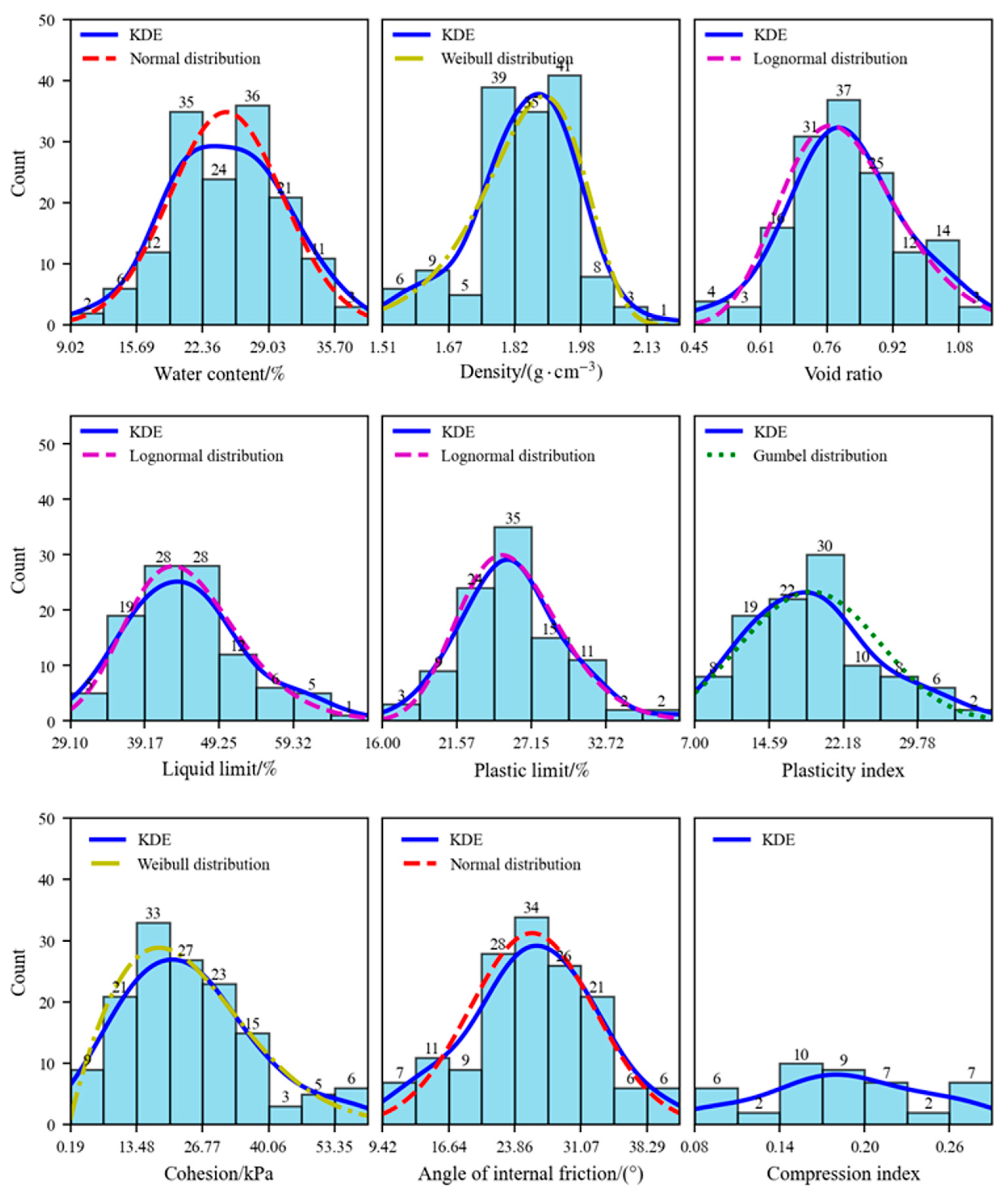
${\chi }^2$, ${\chi }_{\alpha }^2$ and acceptance outcomes for each candidate probability density function are summarized in

Table 2. Statistical table of distribution test results for physical and mechanical parameters of granite residual soil.

		Parameter
		$\mathit{w}/\%$	ρ/g·cm−3	${\mathit{e}}_0$	${\mathit{w}}_{\mathit{L}}/\%$	${\mathit{w}}_{\mathit{p}}/\%$	IP	c/kPa	φ/°	${\mathit{C}}_{\mathit{c}}$
Nor	${\chi }^2$	7.036	24.632	7.195	11.610	6.541	11.989	7.962	10.732	10.301
	${\chi }_{\alpha }^2$	12.592	12.592	12.592	12.592	11.070	11.070	11.070	11.070	7.815
	Decision	Acc.	Rej.	Acc.	Acc.	Acc.	Rej.	Acc.	Acc.	Rej.
Gum	${\chi }^2$	16.801	52.877	11.358	7.763	9.600	7.697	19.218	19.216	2.477
	${\chi }_{\alpha }^2$	12.592	12.592	12.592	12.592	11.070	11.070	11.070	11.070	5.991
	Decision	Rej.	Rej.	Acc.	Acc.	Acc.	Acc.	Rej.	Rej.	Acc.
Wei	${\chi }^2$	8.127	10.023	13.393	18.323	14.147	11.933	6.665	10.473	10.061
	${\chi }_{\alpha }^2$	11.070	11.070	11.070	11.070	9.488	9.488	9.488	9.448	5.991
	Decision	Acc.	Acc.	Rej.	Rej.	Rej.	Rej.	Acc.	Rej.	Rej.
Log	${\chi }^2$	11.888	28.595	4.679	6.351	5.366	8.257	17.227	18.084	2.641
	${\chi }_{\alpha }^2$	11.070	11.070	11.070	11.070	9.488	9.488	9.488	9.488	3.841
	Decision	Rej.	Rej.	Acc.	Acc.	Acc.	Acc.	Rej.	Rej.	Acc.
Adopted Distribution		Nor	Wei	Log	Log	Log	Gum	Wei	Nor	/

Note: Nor = Normal distribution; Gum = Gumbel distribution; Wei = Weibull distribution; Log = Lognormal distribution; Acc. = accepted; Rej. = rejected.

. The corresponding histograms, kernel density estimation (KDE), and adopted distributions are shown in Figure 1. It is worth noting that only 43 samples were available for the compression index, which limits the statistical reliability of the analysis. Therefore, the statistical analysis results for the compression index are for reference only.

The results of the distribution tests indicate that natural density and cohesion approximately follow Weibull distributions; void ratio, liquid limit and plastic limit follow Lognormal distributions; water content and internal friction angle follow Normal distributions; and plasticity index follows a Gumbel distribution.

2.4. Applicability and Limitations of the Chi-Square Test

In this study, probabilistic distribution fitting is used both to characterize the probabilistic features of the physical and mechanical parameters of granite residual soils in the Fujian–Guangdong region and to provide input distribution functions for the subsequent Latin Hypercube Sampling (LHS) in the global sensitivity analysis. Therefore, the main requirement is that the fitted distributions can reasonably capture the overall statistical characteristics of each parameter. It should be noted that different goodness-of-fit tests may lead to slightly different results because they are based on different statistical assumptions and test statistics. The chi-square test is based on grouped frequency differences, and its results may therefore be affected by sample grouping and class interval division. By contrast, the Kolmogorov–Smirnov (K-S) and Anderson–Darling (A-D) tests are based on the cumulative distribution function. For the purpose of this study, the chi-square test is used here as a practical primary method for identifying suitable probability distributions, while the supplementary K-S test results and comparative information are provided in Appendix A.

3. Methods for Sensitivity Analysis

3.1. UH Model

Yao et al. [30] developed the Unified Hardening (UH) model as an improved constitutive model based on the Modified Cam-Clay (MCC) model. The UH model introduces a transformed stress approach and a unified hardening parameter that does not depend on the stress path [31]. Based on the transformed stress concept derived from the SMP criterion [32], the UH model can represent soil strength and deformation under general three-dimensional stress states. The unified hardening parameter enables the model to reproduce diverse soil mechanical behaviors under various loading conditions, including shear dilatancy, overconsolidated behavior, strain hardening and softening, and stress path dependence behavior. The UH model parameters are listed in

Table 3. UH model parameters.

Category	Parameter	Description
Strength parameter	M	Slope of CSL in p × q
State parameter	$e_0$	Void ratio at p = 1 kPa
Stiffness parameter	λ	Slope of NCL in $\ln p\times e$
	κ	Slope of swelling line in $\ln p\times e$
	ν	Poisson’s ratio

.

3.2. Sobol Sensitivity Method

The Sobol method is a widely used global sensitivity analysis technique derived from variance decomposition within the functional analysis of variance (ANOVA) framework. It determines parameter sensitivity by evaluating the extent to which individual input variables influence the variability of the model output. The primary sensitivity measures in this method are the first-order index and the total-effect index.

Consider a model expressed as

$$Y=f\left(X_1,X_2,\dots ,X_n\right)$$

(1)

where Y is the model output and $\mathrm{X}=\left(X_1,X_2,\dots ,X_n\right)$ denotes a vector of $n$ input variables. The total output variance can be decomposed as

$$\mathrm{Var}\left(Y\right)={{\displaystyle \sum }}_{i=1}^n{V}_i+{{\displaystyle \sum }}_{i<j}{V}_{ij}+\cdots +V_{1,2,\dots ,n}$$

(2)

where $V_i$ represents the contribution of the individual effect of $X_i$, $V_{ij}$ denotes the contribution of the interaction between $X_i$ and $X_j$, and higher-order terms account for interactions among multiple variables.

The first-order sensitivity index of the $i$-th $S_i$ variable is defined as

$$S_i={\displaystyle \frac{V_i}{\mathrm{Var}\left(Y\right)}}$$

(3)

which quantifies the direct contribution of $X_i$ to the output variance, excluding interaction effects.

The total effect index of the $i$-th $S_{T_i}$ variable is defined as

$$S_{T_i}=1-{\displaystyle \frac{\mathrm{Var}\left(Y_{-i}\right)}{\mathrm{Var}\left(Y\right)}}$$

(4)

where $\mathrm{Var}\left(Y_{-i}\right)$ denotes the variance of the model output when $X_i$ is fixed, and all other variables are allowed to vary. $S_{T_i}$ measures the overall contribution of $X_i$, including both its main effect and its interactions with other variables.

A larger $S_i$ index indicates a stronger independent influence of a parameter on the model response. Conversely, a relatively small $S_{T_i}$ suggests that the parameter has limited overall impact and may be considered of limited importance for the model output.

3.3. Parameter Distributions

Before performing the Sobol sensitivity analysis of the UH model, it is necessary to define the probability distribution of each input parameter. The distribution types were selected based on the statistical results summarized in Table 1 and Table 2.

$M$ was calculated by $M=6sin\phi /\left(3-sin\phi \right)$ and performed distribution tests. $\lambda$ was obtained through $\lambda =0.434C_c$ [33]. Following Gao [34], the ratio between $\kappa$ and $\lambda$ for typical clays ranges from 0.1 to 0.2. For sampling purposes, the sampling range of $\kappa$ in this study was approximately defined as $\left[0.15{\lambda }_{min},0.15{\lambda }_{max}\right]$, rather than treating $\kappa$ as a fixed value of 0.15λ for each sampled realization. On this basis, the statistical parameters of κ were taken as ${\mu }_{\kappa }=0.15{\mu }_{\lambda }$ and ${\sigma }_{\kappa }^2=0.0225{\sigma }_{\lambda }^2$. ν was assigned with reference to Foti et al. [35]. λ, κ and ν were assumed to follow Normal distributions. The parameter ranges and corresponding distributions adopted in the sensitivity analysis of the UH model are listed in

Table 4. UH model sensitivity analysis input parameter range and distribution.

Parameter	Mean	Range	Distribution
M	1.017	0.346–1.718	Weibull
$e_0$	0.811	0.450–1.157	Lognormal
λ	0.081	0.033–0.128	Normal
κ	0.012	0.005–0.019	Normal
ν	0.29	0.20–0.40	Normal

.

3.4. Method for Parameter Sampling

In global sensitivity analysis, a representative set of input samples must be generated according to the distributions of the model parameters. To enhance sampling efficiency and improve coverage of the parameter space, Latin Hypercube Sampling (LHS) [36] was adopted.

In the LHS approach, the range of each parameter is divided into equally probable, non-overlapping intervals, from which a random sample is drawn.

This stratified sampling strategy ensures systematic exploration of the full range of each variable, resulting in a more uniformly distributed sample set in high-dimensional parameter space compared with conventional random sampling.

4. Results and Discussions

4.1. Baseline Numerical Model

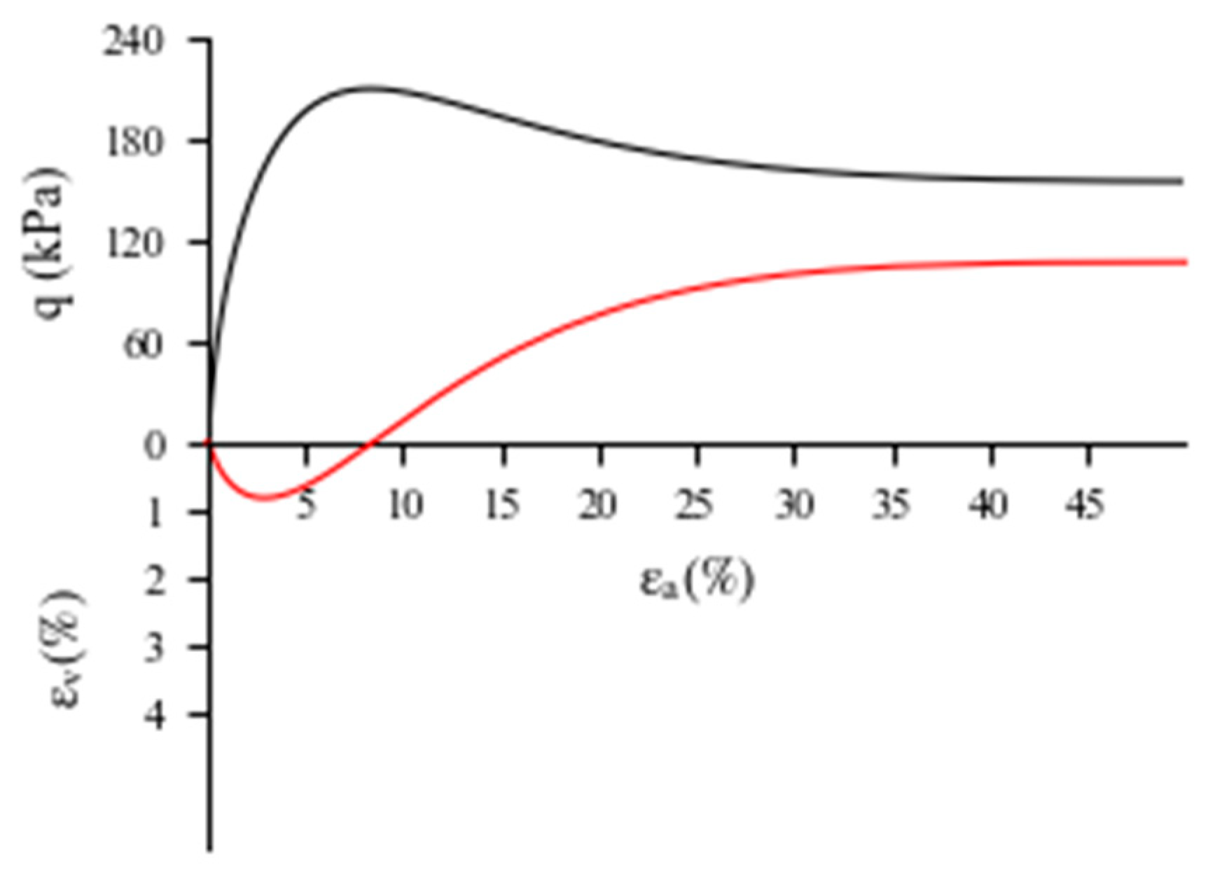
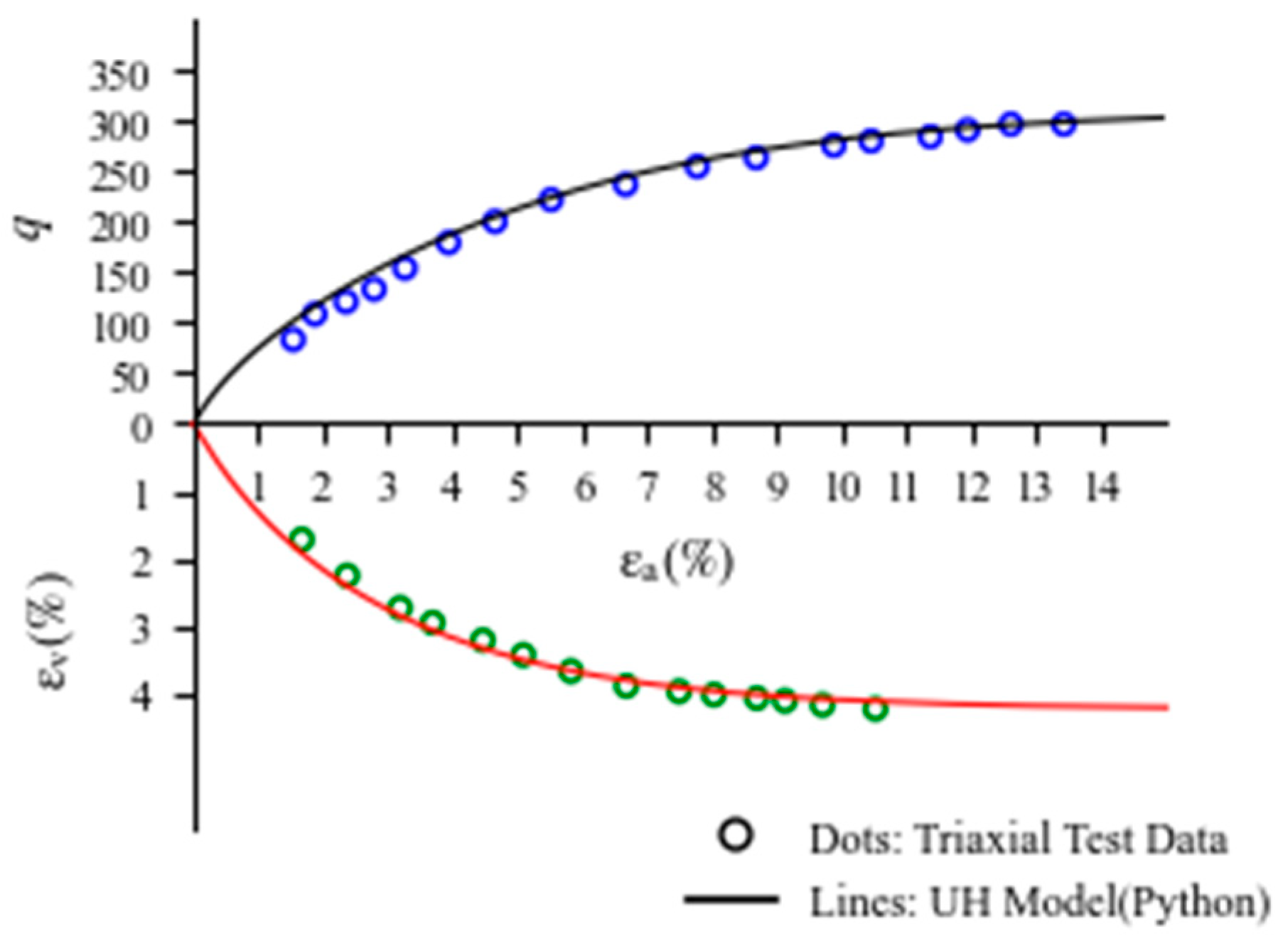
The UH model was numerically implemented in Python3.10 for the present study. To verify the correctness of the implementation and its applicability to granite residual soils, the numerical predictions were compared with triaxial test data on granite residual soil [37]. As shown in Figure 2, there was good agreement between the test data and numerical predictions, including the stress–strain relation and volumetric strain evolution. Based on the above validation, the UH model can be considered suitable for simulating the mechanical behavior of granite residual soil. A drained triaxial compression test on granite residual soil under $p_0=100 \mathrm{kPa}$ and $\mathrm{OCR}=4$ was used as the baseline numerical model for sensitivity analysis. The input parameters were taken as the mean values of the collected data, and

Table 5. Calculation parameters of granite residual soil.

M	${\mathit{e}}_0$	λ	κ	ν
1.017	0.811	0.081	0.012	0.29

summarizes the values of the parameters used in the model. The corresponding simulated stress–strain relations from the baseline model are shown in Figure 3.

4.2. Convergence Analysis of Sample Size

The results of the global sensitivity analysis are closely related to the sample size N. Since different analysis methods and model problems may require different sample sizes, a convergence analysis of the sensitivity results is necessary.

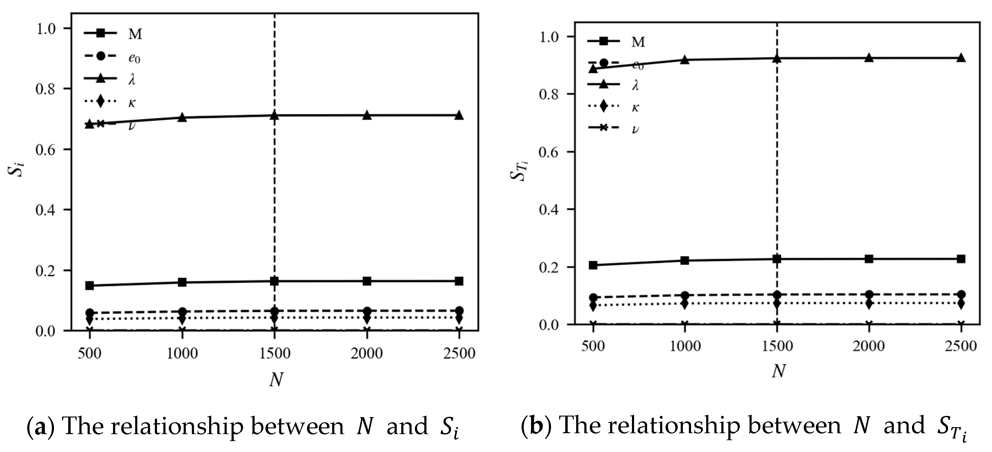
In this study, the mean squared error of ${\epsilon }_v$ was selected as the representative model output for the convergence analysis, because this output is influenced by relatively strong interactions among input parameters and is therefore more demanding in terms of sample size in the Sobol analysis. The initial sample size was set to 500, and then increased in increments of 500 to examine the convergence behavior of the sensitivity indices. As shown in Figure 4, when $N=1500$, both $S_i$ and $S_{T_i}$ become essentially stable, and no significant change is observed with further increases in sample size. This indicates that the sensitivity results are converged and sufficiently stable for the present analysis. Therefore, $N=1500$ was adopted as the sample size for the Sobol sensitivity analysis in this study.

4.3. Results of Sensitivity Analysis

This study selects different physical quantities as model outputs and performs multiple Sobol sensitivity analyses on the UH model parameters to investigate how parameter sensitivity varies under different loading conditions.

4.3.1. Deviatoric Stress at Critical State $q_{cs}$ as Model Output

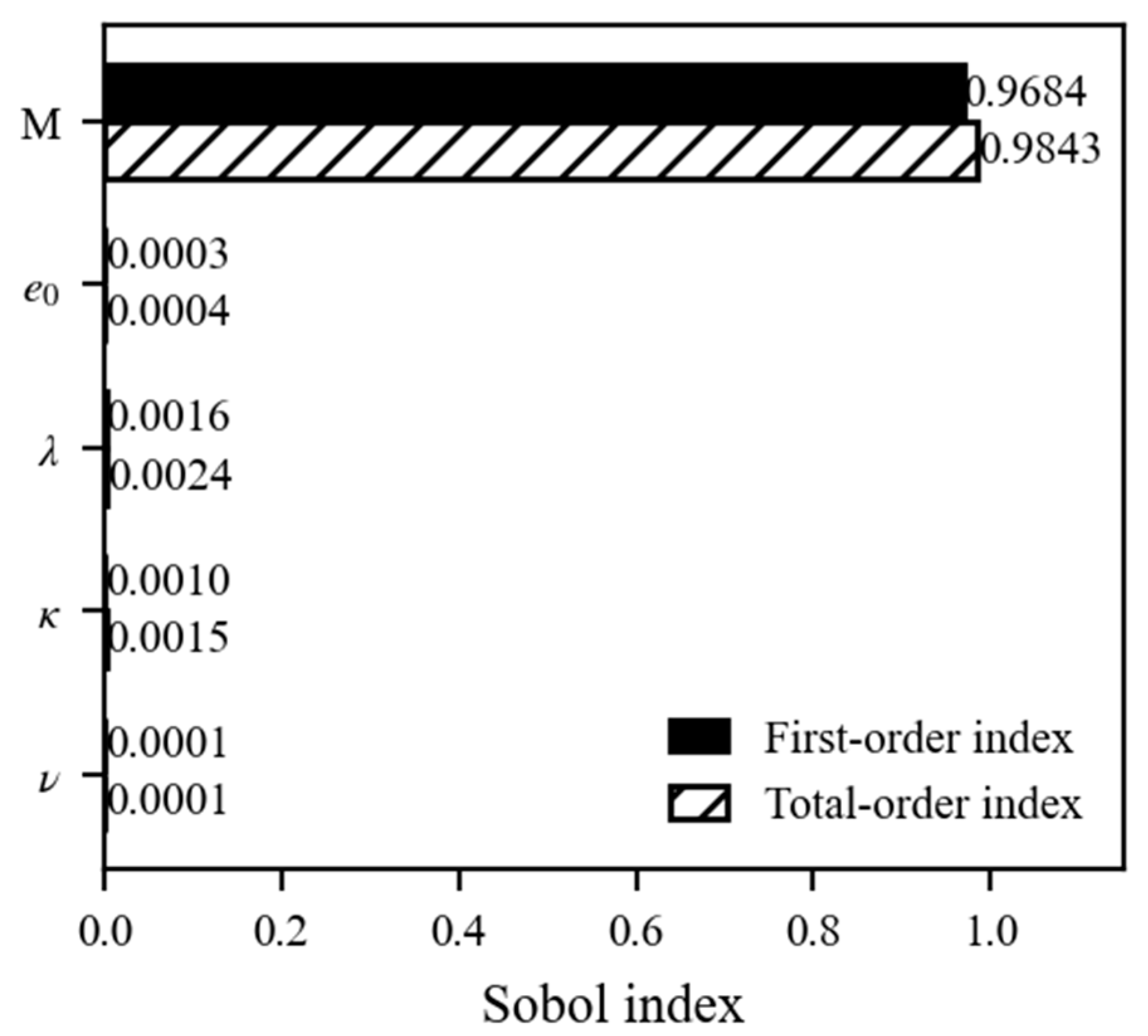
$q_{cs}$ is of particular importance in engineering scenarios dominated by strength considerations, such as slope stability and tunnel excavation. The corresponding Sobol sensitivity indices of the UH model parameters are presented in Figure 5. The $S_i$ and $S_{T_i}$ of $M$ are 0.9684 and 0.9843. In contrast, the $S_i$ and $S_{T_i}$ of the remaining parameters are close to zero.

4.3.2. Volumetric Strain at Critical State ${\epsilon }_{v,cs}$ as Model Output

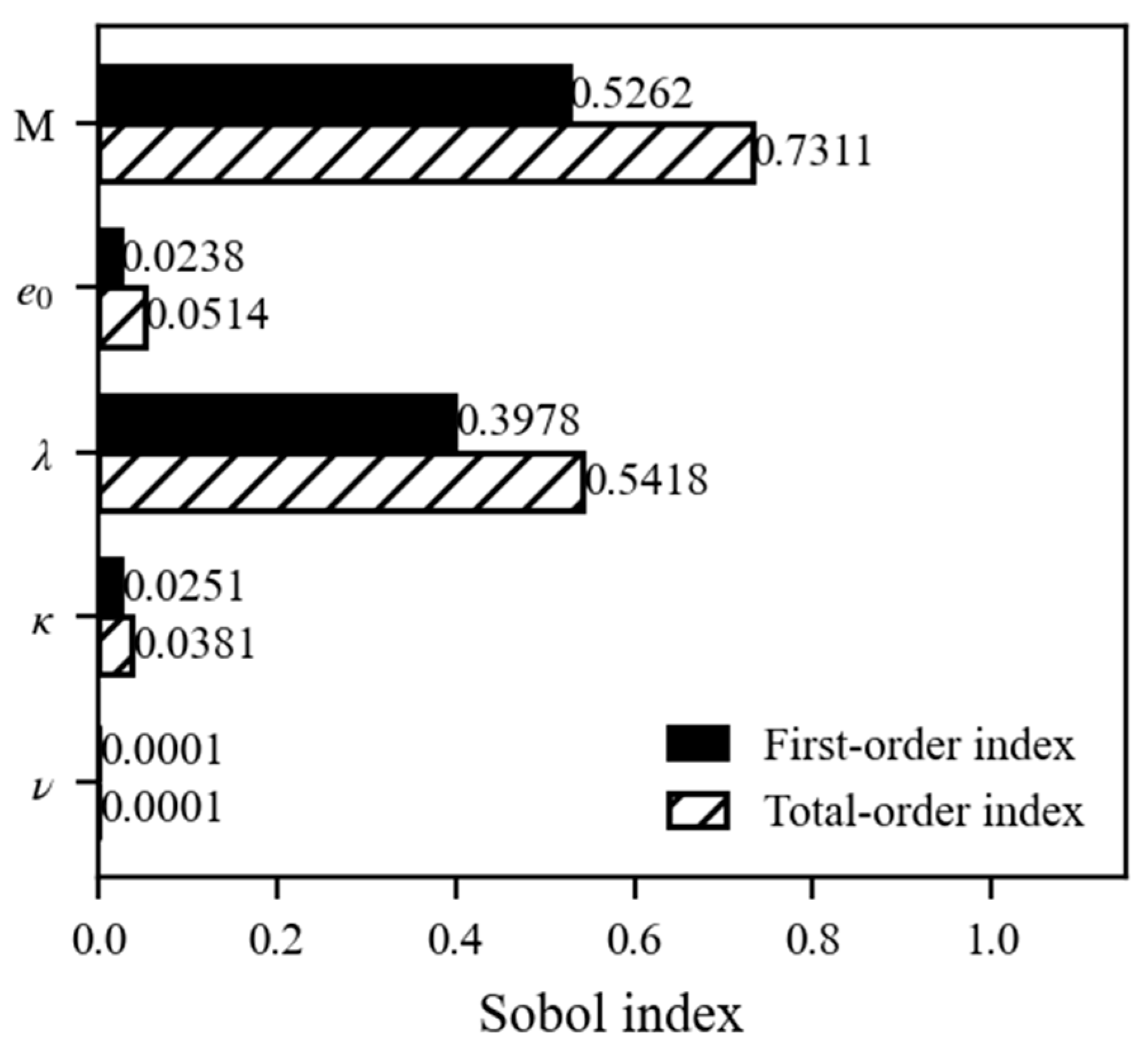
${\epsilon }_{v,cs}$ is particularly important in engineering scenarios where deformation governs performance, such as under cyclic or dynamic loading conditions. The corresponding Sobol sensitivity indices are presented in Figure 6. The $S_i$ and $S_{T_i}$ of M are 0.5262 and 0.7311. the $S_i$ and $S_{T_i}$ of λ are 0.3978 and 0.5418. $e_0$ and κ show small sensitivity indices, and $S_i$ and $S_{T_i}$ of ν are close to zero.

4.3.3. The Mean Squared Error of Deviatoric Stress $q$ as Model Output

The mean squared error (MSE) was employed to quantify the overall discrepancy between simulated responses and reference results. It is defined as

$$\mathrm{MSE}={\displaystyle \frac{1}{N}}{{\displaystyle \sum }}_{i=1}^N{\left(y_i^{\mathrm{ref}}{y}_i^{\mathrm{sim}}\right)}^2$$

(5)

where $y_i^{\mathrm{ref}}$ and $y_i^{\mathrm{sim}}$ denote the $i$-th reference and simulated values, respectively, and $N$ is the total number of data points.

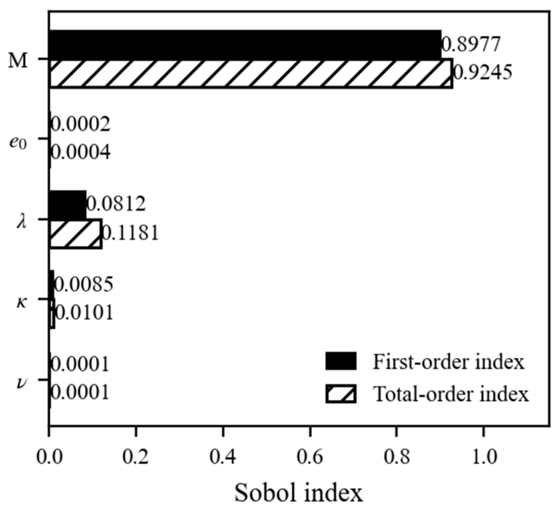
In this analysis, $y_i^{\mathrm{ref}}$ is the $i$-th $q$ obtained from the baseline numerical model. Using the MSE of $q$ as the model output reflects how overall stress deviations vary with parameter changes and how they deviate from the baseline model. The resulting Sobol sensitivity indices are shown in Figure 7. The $S_i$ and $S_{T_i}$ of $M$ are 0.8977 and 0.9245, whereas those of $\lambda$ are 0.0812 and 0.1181. The corresponding indices of the remaining parameters are close to zero.

4.3.4. The Mean Squared Error of Volumetric Strain ${\epsilon }_v$ as Model Output

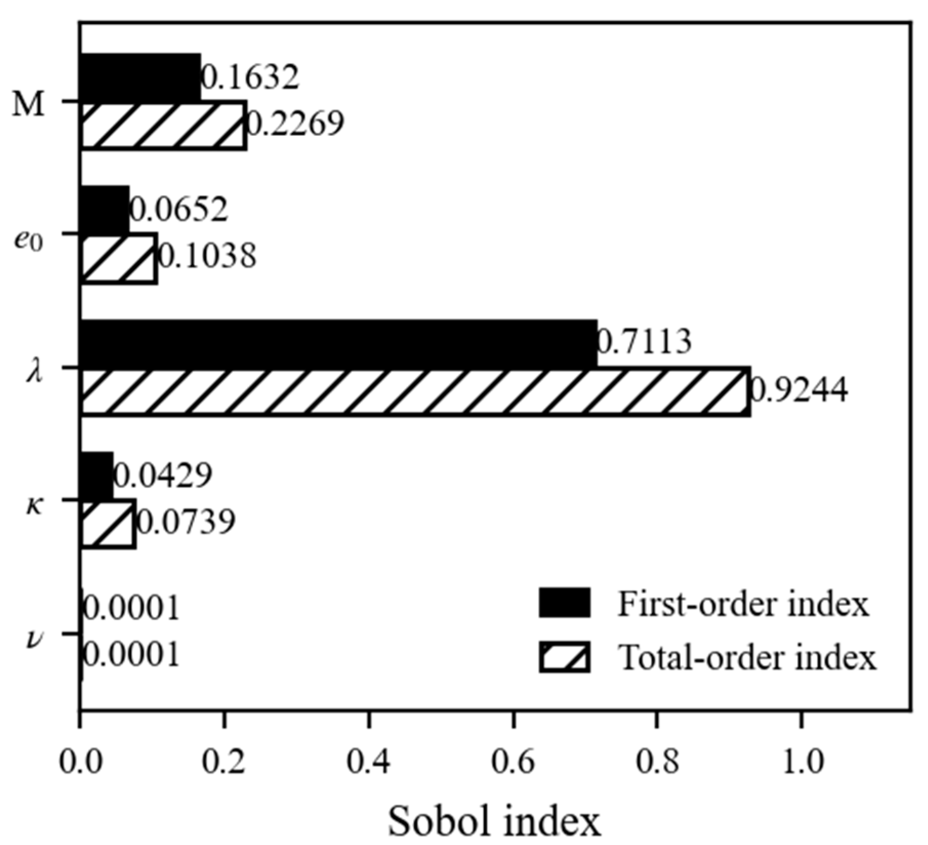
Consistent with Section 4.3.3, the MSE is adopted as the model output; in this case, $y_i^{\mathrm{ref}}$ is the $i$-th ${\epsilon }_v$ obtained from the baseline numerical model. Using the MSE of ${\epsilon }_v$ as the model output reflects how overall volumetric strain varies with parameter changes and how they deviate from the baseline model. The resulting Sobol sensitivity indices are presented in Figure 8. The $S_i$ and $S_{T_i}$ of λ are 0.7113 and 0.9244. The corresponding indices of M are 0.1632 and 0.2269. $e_0$ and κ show low sensitivity indices, and $S_i$ and $S_{T_i}$ of ν are close to 0.

4.4. Discussions of Results

(1)

When $q_{cs}$ is taken as the model output, the $M$ demonstrates the highest sensitivity. According to critical state soil mechanics, we can know $q_{cs}=M{p}_{cs}$; under drained triaxial conditions, we can know $\mathsf{\Delta }q=3\mathsf{\Delta }p$, so we can find the confining pressure at the critical state $p_{cs}=3p_0/\left(3-M\right)$. Therefore, once $p_0$ and $M$ are specified, the $q_{cs}$ is determined. This fundamental relationship accounts for the dominant contribution of $M$ identified in the Sobol sensitivity analysis.

(2)

When ${\epsilon }_{v,cs}$ is considered as the model output, according to critical state soil mechanics, the critical state void ratio is uniquely related to $p_{cs}$ through the critical state line (CSL). CSL is almost parallel to the NCL, thus λ and M which affects $p_{cs}$ jointly influence ${\epsilon }_{v,cs}$.

(3)

When the MSE of q is taken as the model output, M remains the most sensitive parameter. MSE measures the overall deviation of the curve, which corresponds to the evolutionary difference throughout the entire process from the initial state to the critical state in the soil stress–strain curve. M determines the shape of the yield surface, thereby controlling the variation in q during loading. Consequently, M significantly influences this model output.

(4)

When the MSE of ${\epsilon }_v$ is taken as the model output, λ demonstrates the highest sensitivity. λ and κ determine the bulk modulus, thereby controlling the volume deformation characteristics of the soil during its evolution from the initial state to the critical state. Since this evolution is dominated by plastic deformation, the model output is more strongly affected by λ, which primarily governs the plastic volumetric response.

(5)

Among the four model outputs, the $S_i$ and $S_{T_i}$ of $\nu$ are both close to 0, indicating that it has virtually no influence on the model outputs. This is because the model outputs primarily generate large deformations dominated by plastic deformation, whereas ν primarily governs elastic deformation.

(6)

The sensitivity results have direct implications for the calibration and practical application of the UH model. The highly sensitive parameters $M$ and λ should be prioritized during calibration, since small variations in these parameters can lead to pronounced changes in the predicted responses. Specifically, $M$ should be more carefully calibrated for the deviatoric stress response, whereas λ should be more tightly constrained when volumetric deformation is of primary concern. By contrast, the sensitivity of ν is close to zero for all considered outputs, indicating limited information for its reliable identification from the measured data. Therefore, ν may be fixed at an empirical or literature-recommended value rather than treated as a key calibration parameter. Such a sensitivity-based strategy helps reduce the number of parameters requiring intensive calibration, lower calibration uncertainty, and improve the reliability of UH model predictions in practical engineering applications.

5. Conclusions

(1)

The statistical evaluation of eight commonly used physical and mechanical parameters of granite residual soils in the Fujian–Guangdong region demonstrates that, at a conventional significance level α = 0.05, most parameters deviate from normal distributions. Natural density and cohesion approximately follow Weibull distributions; void ratio, liquid limit and plastic limit follow Lognormal distributions; water content and internal friction angle follow Normal distributions; and plasticity index follows a Gumbel distribution. These results highlight the pronounced non-normality and parameter variability of granite residual soils. This regional statistical characterization provides a basis for parameter selection in the Fujian–Guangdong region.

(2)

It should be noted that different goodness-of-fit tests may yield slightly different distribution selections because they emphasize different aspects of distribution fitting. In this study, the chi-squared test is used as the primary method to characterize the overall probabilistic features of the regional parameters and to define the input distributions for the subsequent LHS-based analysis. Its applicability and limitations are discussed in Section 2.4, and supplementary K-S test results are provided in Appendix A.

(3)

The sensitivity analysis demonstrates that, when the UH model applies to granite residual soils in the Fujian–Guangdong region, the parameters $M$ and λ play dominant roles in controlling the simulation results. $M$ primarily governs the $q_{cs}$ as well as the overall evolution of deviatoric stress, whereas λ predominantly controls the evolution of volumetric strain. Both parameters jointly determine ${\epsilon }_{v,cs}$. Accordingly, the required level of calibration accuracy for $M$ and λ should be tailored to the governing engineering conditions in order to enhance the reliability of numerical predictions. By contrast, ν exhibits negligible sensitivity and may be assigned using conventional empirical values in practical engineering applications.

References

1. de Oliveira, I.A.; de Freitas, L.; de Aquino, R.E.; Casagrande, J.C.; Campos, M.C.C.; Silva, L.S. Chemical and physical pedoindicators of soils with different textures: Spatial variability. Environ. Earth Sci. 2018, 77, 81. [Google Scholar] [CrossRef]
2. Paterson, S.; Minasny, B.; McBratney, A. Spatial variability of Australian soil texture: A multiscale analysis. Geoderma 2018, 309, 60–74. [Google Scholar] [CrossRef]
3. Ching, J.; Phoon, K.K. Correlations among some clay parameters—The multivariate distribution. Can. Geotech. J. 2014, 51, 686–704. [Google Scholar] [CrossRef]
4. Löfman, M.S.; Korkiala-Tanttu, L.K. Transformation models for the compressibility properties of Finnish clays using a multivariate database. Georisk 2022, 16, 330–346. [Google Scholar] [CrossRef]
5. Kirts, S.; Panagopoulos, O.P.; Xanthopoulos, P.; Nam, B.H. Soil-compressibility prediction models using machine learning. J. Comput. Civ. Eng. 2018, 32, 04017067. [Google Scholar] [CrossRef]
6. Dai, J.; Gao, G.Y.; Wang, T.H. Regional differences of granitic residual soil and research on its engineering characteristics. Port. Eng. Technol. 2009, 46, 56–59. (In Chinese) [Google Scholar] [CrossRef]
7. Liang, S.H.; Zhou, S.Z.; Zhang, L.; Wang, M. Statistical Analysis of Physical and Mechanical Indexes of Granite Residual Soil in Eastern Guangzhou. J. Guangdong Univ. Technol. 2015, 32, 29–33. (In Chinese) [Google Scholar] [CrossRef]
8. Zhang, J.; Hu, J.Z.; Ma, J.Z.; Wang, H.; Ding, J.W. Probabilistic model for mechanical properties of completely decomposed granite based on multivariate analysis. Eng. J. Wuhan Univ. 2016, 49, 648–653. (In Chinese) [Google Scholar] [CrossRef]
9. Yu, Y.H. Probabilistic Finite Element Method Based on Spatial Variability for Granite Residual Soil Slopes and Its Application. Master’s Thesis, Huazhong University of Science and Technology, Wuhan, China, 2024. (In Chinese) [Google Scholar] [CrossRef]
10. Li, Z.J.; Zhang, W.; Liu, L. Boosting high-quality development of water conservancy by vigorously developing new quality productive forces—Understanding and thoughts on developing new quality productive forces in the water sector. Water Resour. Dev. Res. 2024, 24, 1–6. (In Chinese) [Google Scholar] [CrossRef]
11. Simpson, B.; Nicholson, D.; Banfi, M.; Grose, B.; Davies, R. Collapse of the Nicoll Highway excavation, Singapore. In Forensic Engineering: From Failure to Understanding: Proceedings of the Two Day International Conference Organised by the Institution of Civil Engineers and Held in London on 2 to 4 December 2008; Thomas Telford Publishing: London, UK, 2009; pp. 1–14. [Google Scholar] [CrossRef]
12. Feng, X.; Yao, Y.P.; Li, R.N.; Huo, H.F. Application of UH model to analysis of deformation of embankment on soft soils. Chin. J. Geotech. Eng. 2017, 39, 25–28. (In Chinese) [Google Scholar] [CrossRef]
13. Zhu, J.G.; Zhao, X.L.; He, S.B.; Tian, Y. Applicability verification of UH model on coarse-grained soil and its application in earth rockfill dam. Rock Soil Mech. 2020, 41, 3873–3881. (In Chinese) [Google Scholar] [CrossRef]
14. Liu, W.; Xu, C.J.; Du, H.D.; Zhu, H.L.; Wang, C.H. Stability analysis of overconsolidated unsaturated red clay slope based on modified UH model. Rock Soil Mech. 2024, 45, 1233–1241. (In Chinese) [Google Scholar] [CrossRef]
15. Wu, X.T.; Yao, Y.P.; Wei, R.; Cui, W.J. Numerical simulation of soil deformation induced by tunnel construction with unified hardening model. Rock Soil Mech. 2025, 46, 1013–1024. (In Chinese) [Google Scholar] [CrossRef]
16. Saltelli, A. Global sensitivity analysis: An introduction. In Proceedings of the 4th International Conference on Sensitivity Analysis of Model Output (SAMO 2004); Elsevier: Amsterdam, The Netherlands, 2004; Volume 27, p. 43. [Google Scholar] [CrossRef]
17. Shi, Y.Z.; Ruan, J.C.; Wu, C.X. Xiamen area typical stratum of HS-Small model for small strain parameters sensitivity analysis. Sci. Technol. Eng. 2017, 17, 100–105. (In Chinese) [Google Scholar] [CrossRef]
18. Xie, D.W.; Guan, F.; Ding, W.Q. Determination and Sensitivity Analysis of the Parameters of Hardening Soil Model with Small Strain Stiffness. China Earthq. Eng. J. 2017, 39, 898–906. (In Chinese) [Google Scholar] [CrossRef]
19. Guo, D.Q. Study on Rebound Mechanism of Foundation Pit and Deformation of Service Piles in Soft Soil Area. Master’s Thesis, Tianjin University, Tianjin, China, 2017. (In Chinese) [Google Scholar]
20. Fang, Y.B. Reliability-Based Stability Analysis Method for Tunnel Surrounding Rock. Doctoral Dissertation, Hunan University, Changsha, China, 2020. (In Chinese) [Google Scholar] [CrossRef]
21. Xu, Z.X. Global Sensitivity Analysis of Influencing Factors on Slope Stability. Doctoral Dissertation, Chongqing University, Chongqing, China, 2020. (In Chinese) [Google Scholar] [CrossRef]
22. Guo, X.F.; Dias, D. Kriging based reliability and sensitivity analysis–Application to the stability of an earth dam. Comput. Geotech. 2020, 120, 103411. [Google Scholar] [CrossRef]
23. Pandit, B.; Kumar, A.; Tiwari, G. Assessing the applicability of local and global sensitivity approaches and their practical utility for probabilistic analysis of rock slope stability problems: Comparisons and implications. Acta Geotech. 2023, 18, 2615–2637. [Google Scholar] [CrossRef]
24. Kumar, A.; Tiwari, G. A re-sampling statistics based imprecise moment independent global sensitivity analysis methodology with limited data of uncorrelated and correlated geotechnical properties. Structures 2024, 70, 107686. [Google Scholar] [CrossRef]
25. Zhang, W.G.; Zhang, R.H.; Han, L.; Goh, A.T.C. Engineering properties of the Bukit Timah Granitic residual soil in Singapore. Undergr. Space 2019, 4, 98–108. [Google Scholar] [CrossRef]
26. Chen, H.J.; Cui, G.Y. Probability type testing of the distribution on the granite eluvial soil mechanical parameters. J. Huazhong Univ. Sci. Technol. 2001, 29, 92–94. (In Chinese) [Google Scholar] [CrossRef]
27. Pearson, K. On the criterion that a given system of deviations from the probable in the case of a correlated system of variables is such that it can be reasonably supposed to have arisen from random sampling. Philos. Mag. 1900, 50, 157–175. [Google Scholar] [CrossRef]
28. Liu, Y.; Zhang, W.; Zhang, L.; Zhu, Z.; Hu, J.; Wei, H. Probabilistic stability analyses of undrained slopes by 3D random fields and finite element methods. Geosci. Front. 2018, 9, 1657–1664. [Google Scholar] [CrossRef]
29. Puente-Sotomayor, F.; Mustafa, A.; Teller, J. Landslide Susceptibility Mapping of Urban Areas: Logistic Regression and Sensitivity Analysis applied to Quito, Ecuador. Geoenviron. Disasters 2021, 8, 19. [Google Scholar] [CrossRef]
30. Yao, Y.P.; Zhou, A.N.; Lu, D.C. Extended transformed stress space for geomaterials and its application. J. Eng. Mech. 2007, 133, 1115–1123. [Google Scholar] [CrossRef]
31. Yao, Y.P.; Hou, W.; Zhou, A.N. UH model: Three-dimensional unified hardening model for overconsolidated clays. Géotechnique 2009, 59, 451–469. [Google Scholar] [CrossRef]
32. Nakai, T.; Hinokio, M. A simple elastoplastic model for sand considering the stress path dependency in three-dimensional stresses. Soils Found. 2004, 44, 53–70. [Google Scholar] [CrossRef] [PubMed]
33. Xu, Z.H. Study on Deformation Behavior of Deep Excavation Combining Retaining Structure with Main Structure in Shanghai area. Doctoral Dissertation, Shanghai Jiao Tong University, Shanghai, China, 2007. (In Chinese) [Google Scholar]
34. Gao, D.Z. Soil Mechanics and Foundation Engineering; China Architecture & Building Press: Beijing, China, 1998. (In Chinese) [Google Scholar]
35. Foti, S.; Passeri, F. Reliability of soil porosity estimation from seismic wave velocities. In Proceedings of International Conference on Geotechnical and Geophysical Site Characterization; Australian Geomechanics Society: Sydney, Australia, 2016; pp. 425–430. [Google Scholar]
36. Loh, W.L. On Latin hypercube sampling. Ann. Stat. 1996, 24, 2058–2080. [Google Scholar] [CrossRef]
37. Liu, P. Experimental Study and Constitutive Model of Completely Decomposed Granite. Doctoral Dissertation, South China University of Technology, Guangzhou, China, 2016. (In Chinese) [Google Scholar]
Figure 1. Histogram, KDE, and fitted distribution of the physical and mechanical parameters of granite residual soil.
Eng 07 00179 g001
Figure 2. Triaxial test data and numerical predictions of the stress–strain relation and volumetric strain from the triaxial tests on granite residual soils.
Eng 07 00179 g002
Figure 3. Drained triaxial test stress–strain curves of the baseline numerical model.
Eng 07 00179 g003
Figure 4. The relationships between N and sensitivity indices.
Eng 07 00179 g004
Figure 5. S i and S T i of the UH model parameters with q c s as the model output.
Eng 07 00179 g005
Figure 6. S i and S T i of the UH model parameters with ε v , c s as the model output.
Eng 07 00179 g006
Figure 7. S i and S T i of the UH model parameters with the MSE of q as the model output.
Eng 07 00179 g007
Figure 8. S i and S T i of the UH model parameters with the MSE of ε v as the model output.
Eng 07 00179 g008