Quick Identification of Single Open-Switch Faults in a Vienna Rectifier

Abstract

Three-leg AC-DC Vienna rectifiers are susceptible to single open-switch faults, which make DC-link voltage ripple and make three-leg input AC currents distorted and unbalanced. Thus, this paper presents a quick identification method for single open-switch faults based on three-leg fault currents and output capacitors voltage difference. Fault-leg identification depended on zero-plateaus in the three-leg fault currents, whereas fault-side identification was dependent on reconstruction variables obtained through Clark transformation and phase shifting. In order to improve the reliability of the diagnosis system, the harmonic component of capacitor voltage difference is used to realize the missed diagnosis detection and adjust the time threshold automatically. This method requires no additional hardware and is easy to implement. Experimental results verify the effectiveness of this strategy. It is shown that the fault diagnosis method proposed in this paper has the advantages of fast diagnosis speed, high accuracy and good robustness.

1. Introduction

The relentless pursuit of higher efficiency, power density, and reliability in power conversion systems has driven the widespread adoption of multilevel converter topologies across critical industrial domains. From renewable energy generation and electric vehicle fast-charging stations to data center power supplies and aerospace electrical systems, the demand for clean, stable, and uninterrupted power is paramount [1,2]. Compared to conventional two-level voltage-source inverters (2L-VSIs), multilevel converters offer inherent advantages, including reduced voltage stress on semiconductor devices, superior output waveform quality with lower harmonic distortion, and the potential for higher efficiency through lower switching losses [3,4]. Among these topologies, the Vienna rectifier occupies a distinctive niche. By employing only three active switches per bridge—half the number required in a standard 2L-VSI—it achieves three-level pulse-width modulation (PWM) operation. This elegant compromise between circuit complexity, component count, and performance has cemented its position as a preferred solution for medium-power applications demanding high power factor, compact size, and cost-effectiveness, such as in telecom rectifiers, industrial motor drives, and aviation ground power units [5,6].

However, the increased reliability promised by fewer active devices is counterbalanced by the heightened criticality of each remaining switch. Semiconductor failures, predominantly arising from thermal overstress or electrical overcurrent, remain a primary cause of power converter downtime [7]. These failures are categorized into short-circuit and open-circuit faults. While short-circuit faults are catastrophic and typically addressed by immediate hardware protection, open-switch faults are more deceptive. They may not cause an instantaneous system shutdown but induce progressive performance degradation, including distorted grid currents, elevated DC-link voltage ripple, and neutral-point voltage imbalance [8]. Prolonged operation under such a fault condition can trigger secondary failures in downstream loads, leading to costly unplanned maintenance and operational hazards [9]. Consequently, the development of fast, accurate, and real-time open-circuit fault diagnosis (OCFD) strategies has become a cornerstone for enhancing system availability, enabling predictive maintenance, and paving the way for fault-tolerant operation.

Extensive research efforts have been devoted to OCFD, yielding methodologies that can be broadly classified into three evolving paradigms. The first and most established paradigm relies on model-based or signal-based analysis of electrical measurements. This includes methods utilizing the normalized average value or derivatives of phase currents [10], the trajectory, angle, or shape of the current vector in stationary (α-β) or synchronous (d-q) reference frames [11,12], and techniques based on the analysis of DC-link voltage ripple patterns [13]. For instance, in three-level neutral-point clamped (NPC) active rectifiers, a diagnostic method utilizing the vector trajectory of the DC-link voltage ripple in conjunction with grid phase information has been proposed to effectively locate faulty inner switches [14]. While often effective, many of these approaches can be limited by their sensitivity to operating point variations (e.g., light loads), susceptibility to noise, diagnostic latency (requiring data from one or more fundamental cycles), or the need for additional voltage sensors.

The second paradigm leverages artificial intelligence (AI) and deep learning (DL) to handle the non-stationary and noisy characteristics of fault signals. These data-driven methods, employing techniques such as optimized long short-term memory networks [15], extreme learning machines [16], and attention mechanisms [17], promise high accuracy and adaptability. A notable advancement for Vienna rectifiers is a hybrid Transformer-BiTCN model, optimized via a metaheuristic algorithm [18]. This method demonstrates remarkable robustness by extracting hierarchical spatiotemporal features. However, the formidable performance of such AI-based diagnostic systems comes at the cost of requiring extensive historical fault data for training, substantial offline and online computational resources, and often results in a “black-box” decision process. For resource-constrained, real-time digital controllers where determinism, simplicity, and rapid response are critical, these requirements can be prohibitive.

Beyond these data-intensive approaches, system-level harmonic impedance analysis represents another diagnostic methodology primarily used for grid disturbance monitoring in multi-converter systems. While effective for identifying harmonic sources and ensuring compliance with grid codes such as IEEE 519 [19], this approach operates on a slower timescale, requires precise grid-side measurements, and provides system-level alerts rather than specific device-level fault localization [20].

Table 1. Comparison of key performance and applicable characteristics of various methods.

Approach	Principle	Speed	Application Scenario	Compliance with Grid Standards
Conventional Signal Analysis (Current/Voltage)	Waveform/trajectory features	Medium (1 + cycles)	Single-unit diagnosis	Indirect (via THD monitoring)
System-level Impedance Analysis	Grid harmonic impedance variation	Slow (steady-state)	Multi-converter systems	Direct (grid code compliance)
AI/Data-driven Methods	Deep learning feature extraction	Medium (inference time)	Complex nonlinear systems	Indirect
Proposed Method	Current zero-plateau + voltage harmonic fusion	Fast (<1/6 cycle)	Embedded real-time control	Direct (prevents violation)

systematically compares these diagnostic paradigms, positioning the proposed method within the broader technical landscape. While system-level impedance analysis excels at grid disturbance monitoring for multi-converter systems, it operates at a slower timescale and provides system-wide alerts rather than precise device-level fault localization [21]. In contrast, the proposed method leverages the unique, immediate electrical signatures within the converter itself—specifically, the instantaneous current zero-plateau and the characteristic harmonic shift in capacitor voltage difference. This ‘inside-out’ approach enables ultra-fast, precise switch-level identification, making it particularly suitable for embedded control applications where rapid response is critical for preventing secondary failures and maintaining power quality compliance

Bridging the gap between the computational complexity of AI methods and the potential limitations of conventional signal analysis, a third direction focuses on developing lightweight, fast, and easily integrable algorithms tailored for specific, high-volume converter topologies like the Vienna rectifier. The core challenge is to identify unique, immediately apparent fault signatures within the standard sensor measurements already available in the control system. Recent work has begun exploring the distinct current distortion patterns, such as the appearance of zero-current plateaus, caused by open-switch faults in Vienna rectifiers [22]. Yet, a comprehensive diagnostic strategy that synergistically combines the instantaneous detection capability of such current signatures with a validating mechanism to ensure reliability under all operating conditions, while remaining entirely free of additional hardware and complex computations, has not been fully established.

To address this need, this paper proposes a novel, quick, and reliable identification method for single open-switch faults in the three-phase Vienna rectifier. The proposed method is fundamentally a fast model-based primary diagnosis coupled with a simple data-driven verification step, all executed within the standard control loop. The primary diagnosis exploits the immediate appearance of a zero-current plateau in the faulted phase, enabling leg identification within a fraction of a cycle. Subsequently, a straightforward Clark transformation with a fixed phase shift is applied to determine the faulty switch (upper or lower). To guard against rare, missed detections—particularly at very low modulation ratios—a secondary, validating stage monitors the harmonic composition of the capacitor voltage difference. This stage can confirm the diagnosis or trigger an adaptive adjustment of the detection threshold, thereby creating a highly reliable diagnostic system. The entire algorithm uses only the existing phase currents and DC-link capacitor voltages, requires no additional sensors or complex training, and is designed for direct implementation in a standard microcontroller or DSP.

The main contributions of this work are summarized as follows:

• It provides a detailed analysis of the instantaneous current (zero plateau) and DC-link capacitor voltage harmonic signatures specific to single open-switch faults in the three-leg Vienna rectifier.
• It proposes a fast two-stage diagnostic algorithm that combines the speed of instantaneous current feature extraction with the reliability of voltage harmonic validation.
• It incorporates an adaptive threshold adjustment triggered by the voltage-based verification to ensure robustness across a wide range of operating points, including challenging low-modulation-ratio conditions.
• The method’s effectiveness, speed, and robustness are rigorously validated through both simulations and experimental tests under various fault locations, modulation indices, and fault inception angles.

It establishes clear connections to grid code compliance requirements and industrial application contexts, demonstrating practical relevance beyond academic novelty.

The remainder of this paper is organized as follows: Section 2 details the operational analysis and fault signature study. Section 3 elaborates on the proposed diagnostic algorithm. Section 4 presents the simulation and experimental verification, with dedicated correlation analysis between theoretical predictions and measured results. Finally, Section 5 concludes the paper and discusses future work, including industrial implementation considerations.

2. Analysis of Single Open-Switch Faults in Vienna Rectifiers

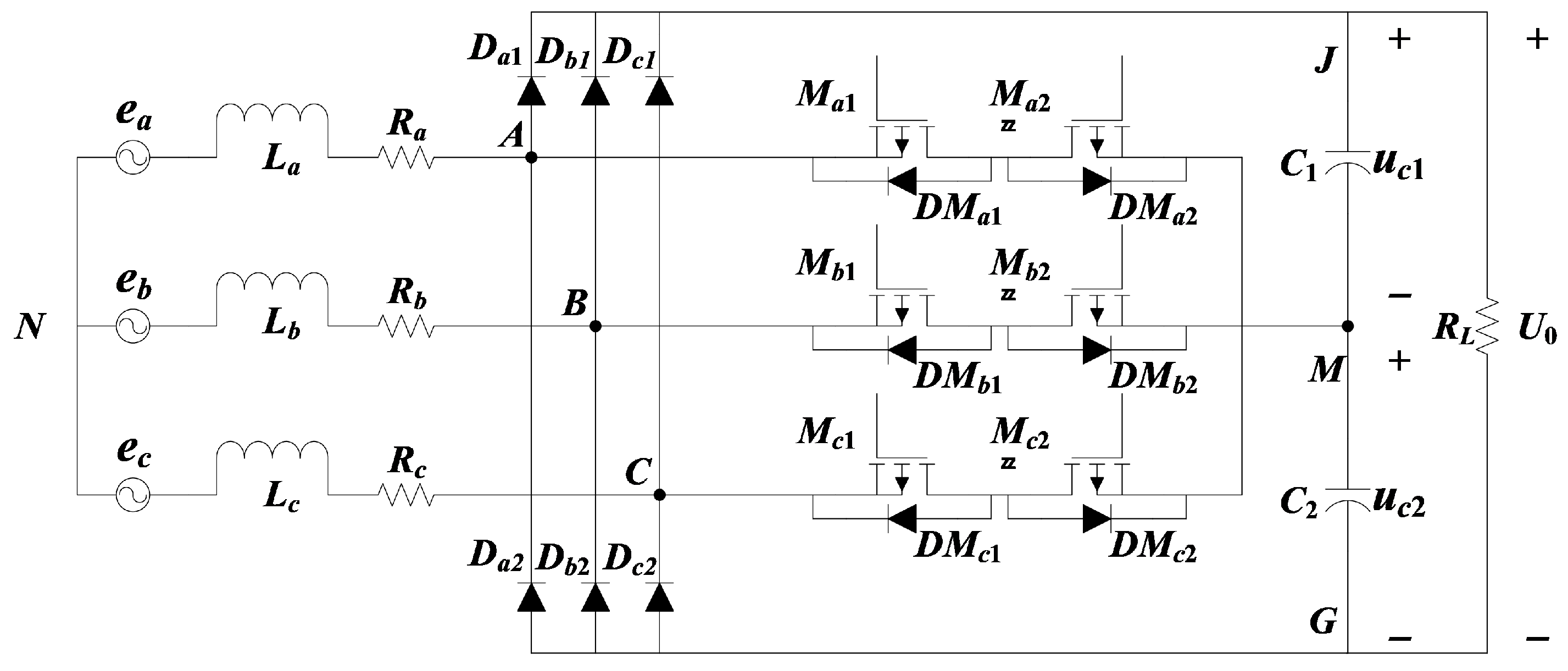
The topology of a typical three-leg Vienna rectifier, under single-cycle control, is shown in Figure 1. Referring to Figure 1, L_a, L_b, and L_c are the inductors of the input filter; R_a, R_b, and R_c are the equivalent series resistances of the inductors of the input filter; D_kj, M_kj, and DM_kj (k = a, b, c; j = 1, 2) are rectifier diodes, power switches, and freewheeling diodes connecting MOSFETs in parallel, respectively; C₁ and C₂ are the balance capacitors on the DC side; R_L is a load resistor; e_a, e_b, e_c and i_a, i_b, i_c are three-leg voltages and three-leg currents at the network side, respectively; u_C1 and u_C2 are the voltages of the balance capacitors; U_o is the voltage at the DC output-sides.

2.1. Operation of Vienna Rectifiers

Two power switches on each leg of the Vienna rectifier were connected in reverse series and controlled by the same driving signal to avoid being turned on at the same time. The switching state of each phase can be represented by the switching function S_k (k = a, b, c):

$$S_k=\left\{\begin{array}{ll}0,& \mathrm{while} {\mathrm{M}}_{k1} \mathrm{turn}\text{-}\mathrm{off}, {\mathrm{M}}_{k2}\mathrm{turn}\text{-}\mathrm{off}\\ 1,& \mathrm{while} {\mathrm{M}}_{k1} \mathrm{turn}\text{-}\mathrm{on}, {\mathrm{M}}_{k2}\mathrm{turn}\text{-}\mathrm{off}\\ -1,& \mathrm{while} {\mathrm{M}}_{k1} \mathrm{turn}\text{-}\mathrm{off}, {\mathrm{M}}_{k2}\mathrm{turn}\text{-}\mathrm{on}\end{array}\right..$$

(1)

During normal operation, the switching state variable S_k fetches 1 or −1. The three-leg input currents follow the three-leg input voltage, keeping the frequency and angle of current i_k same with that of voltage e_k. The output voltage U_o is constant and the voltage neutral-point M balanced. The boost ratio κ is given as follows:

$$\kappa ={\displaystyle \frac{U_o}{U}}.$$

(2)

where U is AC input voltage on the network side. When single open-switch fault occurs, the faulty switch does not turn on and the switching state variable of the faulty leg is locked on 0 or 1/−1. Three-leg currents are distorted but three-leg voltages remain the same as in normal operation.

2.2. Single Open-Switch Fault Current in Vienna Rectifiers

The MATLAB/Simulink (R2022B) simulation model of the Vienna rectifier, shown in Figure 1, is set up to extract open-switch faults. The properties of the model are listed in

Table 2. Properties of Vienna rectifier MATLAB/Simulink simulation model.

Parameter Symbol	Value
Input Filter Inductors La, Lb, Lc	2 mH
Equivalent Series Resistance Ra, Rb, Rc	0.1 Ω
Rectifier Diodes Dkj	Ron = 0.001 Ω
Power Switches Mkj	Ron = 0.1 Ω
Freewheeling Diodes DMkj	Rd = 0.01 Ω
DC-side Capacitors C1, C2	680 uF
Load Resistor RL	60 Ω
AC side input voltage U	20–30 V
DC side output voltage Uo	100 V
Output Power	166.7 W
Switching Frequency	20 kHz

The boost ratio κ is changed by adjusting input voltage U. A time relay is introduced into the drive circuit of the faulty switch and its delay time is controlled to simulate fault occurrence at fault trigger angle θ_f, which is defined as the angle of phase A when a fault occurs.

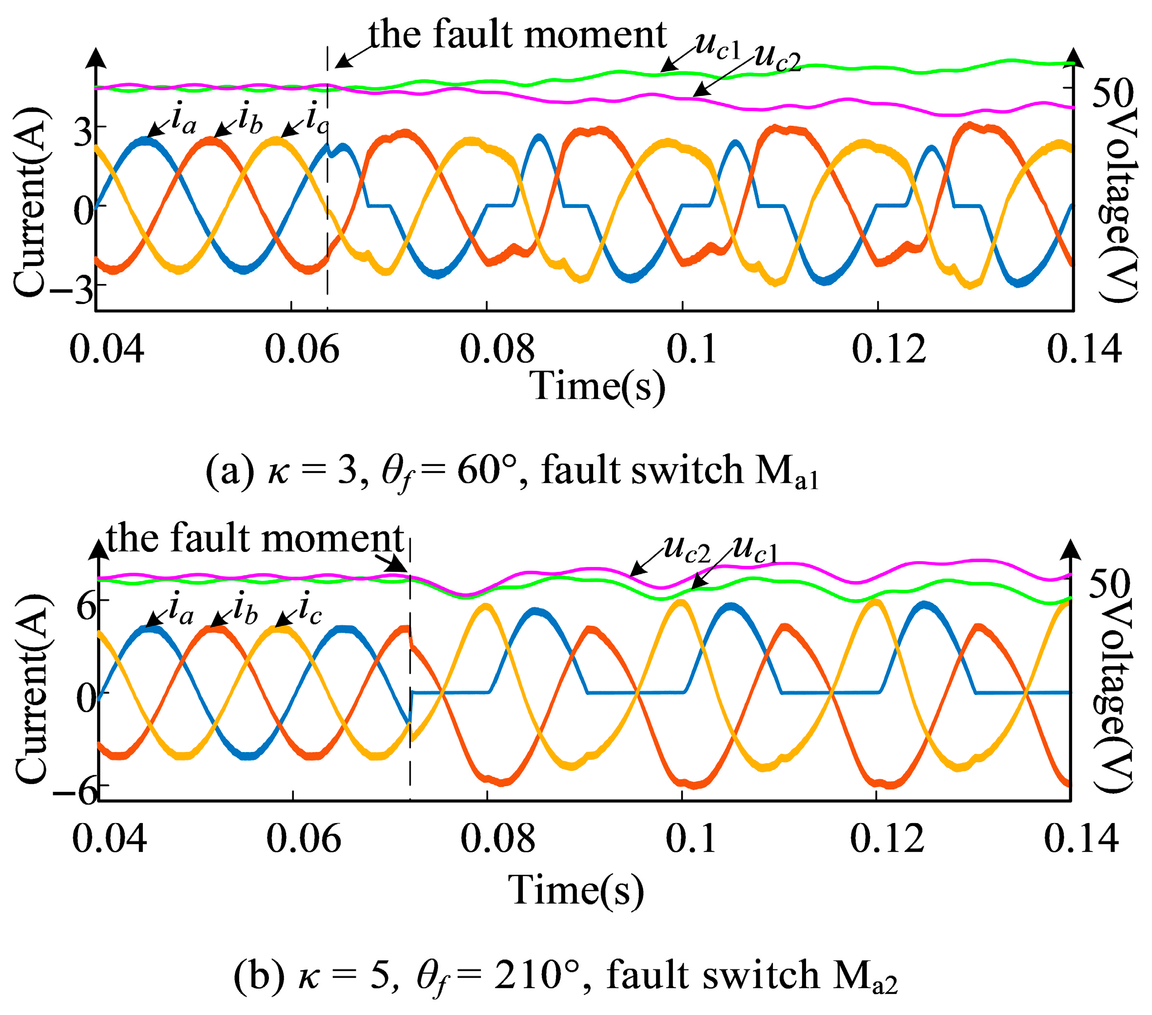
The model was simulated under six instances of single open-switch faults. i_a, i_b, i_c, u_C1, u_C2, and U_o were monitored before and after faults. Some of the simulation results are shown in Figure 2.

The simulation results showed that the fault-leg current i_k had an obvious zero-plateau (with and without a sharp pulse) in the positive cycle for faults in M_k1, and an obvious zero-plateau in the negative cycle for faults in M_k2.

Taking M_a1 as the faulty switch, the main reasons for the zero-plateau in the fault-leg current are as follows:

(1)

When the electrical angle θ ranges from 0° to 180°, the switch M_a2 remains turned off and there is a current path along A → M_a1 → DM_a2 → M because switch M_a1 can be turned on and S_a = 1. If open-circuit fault occurs at M_a1 during the half cycle, the current path will be broken because M_a1 cannot be turned on and S_a = 0. If e_a is not sufficient to turn on the rectifier diode D_a1, i.e., u_AN − u_JN < 0.7 V, there will be no path for current i_a and there is a zero-plateau without a sharp pulse in the positive half cycle. If e_a is sufficient to turn on D_a1, i.e., u_AN − u_JN > 0.7 V, the current i_a flows through D_a1 and there is a sharp pulse in the middle of the zero-plateau of current i_a.

(2)

When the electrical angle θ is between 180° and 360°, switch M_a1 remains turned off and M_a2 can be turned on or off. The switching state S_a can be 0 or −1. There is no need in switching on M_a1 in the half cycle, so single open-switch faults in M_a1 have no influence on current paths.

(3)

According to Kirchhoff’s current law (KCL), i_a + i_b + i_c = 0. When there is a zero-plateau in the fault-leg current, the currents in the other two fault-free legs are opposite. Severe distortion of the fault-leg current leads to slight distortion in the current of the two fault-free legs.

The critical boost ratio κ_th was accurately determined as 4.64 by changing the boost ratio κ in the simulation. The pulse width of the spike t_pmax was determined as 5 ms by monitoring the three-leg input currents.

2.3. Single Open-Switch Fault Voltage in Vienna Rectifiers

This section analyzes the harmonics of capacitor voltage difference in Vienna rectifiers. The three-phase input current is as:

$$\left\{\begin{array}{l}{i}_{\mathrm{LA}}=I_{\mathrm{m}}\sin ({\omega }_{0}t)\\ i_{\mathrm{LB}}=I_{\mathrm{m}}\sin ({\omega }_{0}t-2\pi /3)\\ i_{\mathrm{LC}}=I_{\mathrm{m}}\sin ({\omega }_{0}t+2\pi /3)\end{array}\right.$$

(3)

where I_m is the input current amplitude.

The fundamental component of three-phase voltage switching function is as:

$$\left\{\begin{array}{l}{d}_a=\mathrm{sgn}(i_{\mathrm{LA}})(1-J_a)=M\sin ({\omega }_{0}t)\\ d_b=\mathrm{sgn}(i_{\mathrm{LB}})(1-J_b)=M\sin ({\omega }_{0}t-2\pi /3)\\ d_c=\mathrm{sgn}(i_{\mathrm{LC}})(1-J_c)=M\sin ({\omega }_{0}t+2\pi /3)\end{array}\right.$$

(4)

where M is the modulation ratio, J_k is the fundamental component of the switching function and sgn (i) is the sign function, the value of which is 1 when i is greater than zero, and −1 when i is less than zero.

The current flowing through freewheeling diodes in each leg is as:

$$\left\{\begin{array}{l}{i}_{Da1}=\left\{\begin{array}{ll}(1-J_a)i_{\mathrm{LA}},& i_{\mathrm{LA}}\ge 0\\ 0,& i_{\mathrm{LA}}<0\end{array}\right.\\ i_{Da2}=\left\{\begin{array}{ll}-(1-J_a)i_{\mathrm{LA}},& i_{\mathrm{LA}}<0\\ 0,& i_{\mathrm{LA}}\ge 0\end{array}\right.\\ i_{Db1}=\left\{\begin{array}{ll}(1-J_b)i_{\mathrm{LB}},& i_{\mathrm{LB}}\ge 0\\ 0,& i_{\mathrm{LB}}<0\end{array}\right.\\ i_{Db2}=\left\{\begin{array}{ll}-(1-J_b)i_{\mathrm{LB}},& i_{\mathrm{LB}}<0\\ 0,& i_{\mathrm{LB}}\ge 0\end{array}\right.\\ i_{Dc1}=\left\{\begin{array}{ll}(1-J_c)i_{\mathrm{LC}},& i_{\mathrm{LC}}\ge 0\\ 0,& i_{\mathrm{LC}}<0\end{array}\right.\\ i_{Dc2}=\left\{\begin{array}{ll}-(1-J_c)i_{\mathrm{LC}},& i_{\mathrm{LC}}<0\\ 0,& i_{\mathrm{LC}}\ge 0\end{array}\right.\end{array}\right..$$

(5)

According to Kirchhoff law, the relationship between capacitor voltage difference and current is as:

$$C_f{\displaystyle \frac{d(U_{C1}-U_{C2})}{dt}}=C_f{\displaystyle \frac{d\Delta U}{dt}}=\underset{i}{\Sigma }(i_{Di1}-i_{Di2}) (i=a,b,c)$$

(6)

where C_f is the output capacitance.

Combining Equation (3) with Equation (6), the voltage difference is as:

$$C_f{\displaystyle \frac{d\Delta U}{dt}}=d_a\left|i_{\mathrm{LA}}\right|+d_b\left|i_{\mathrm{LB}}\right|+d_c\left|i_{\mathrm{LC}}\right|$$

(7)

$$\Delta U\approx {\displaystyle \frac{M}{6{\omega }_0{C}_f}}{I}_m\cos (3{\omega }_{0}t).$$

(8)

Equation (8) shows that under normal conditions the main harmonic component of the capacitor voltage difference is the third harmonic.

When a single open-switch fault occurs, the fault-leg current has two states: zero-plateau and sharp pulse. Assuming that M_a1 is faulty and the current is in zero-plateau, both the switch and freewheeling diode are not conductive. The current flowing through the freewheeling diode D_a1 is as:

$$i_{D_{a1}}=0.$$

(9)

The voltage difference ΔU is deduced from Equations (3), (4), (7) and (9) as:

$$\Delta U\approx {\displaystyle \frac{M{I}_m}{C_f}}(-t+{\displaystyle \frac{1}{4{\omega }_0}}\sin 2{\omega }_{0}t+{\displaystyle \frac{1}{6{\omega }_0}}\cos 3{\omega }_{0}t).$$

(10)

Equation (21) shows that the DC component and the second harmonic in the capacitor voltage difference will increase when the current is in zero-plateau.

When the current is sharp pulse, the current flowing through the freewheeling diode D_a1 is as:

$$i_{Da1}=i_{\mathrm{LA}}.$$

(11)

The voltage difference ΔU is deduced from Equations (3), (4), (7) and (11) as:

$$\Delta U\approx {\displaystyle \frac{M{I}_m}{C_f}}(-t-{\displaystyle \frac{1}{M{\omega }_0}}\cos {\omega }_{0}t+{\displaystyle \frac{1}{4{\omega }_0}}\sin 2{\omega }_{0}t+{\displaystyle \frac{1}{6{\omega }_0}}\cos 3{\omega }_{0}t).$$

(12)

Equation (12) shows that the DC component, the first and the second harmonic in the capacitor voltage difference will increase when the current is sharp pulse.

3. The Proposed Identification Method and Its Implementation

3.1. Identification Method for Single Open-Switch Faults

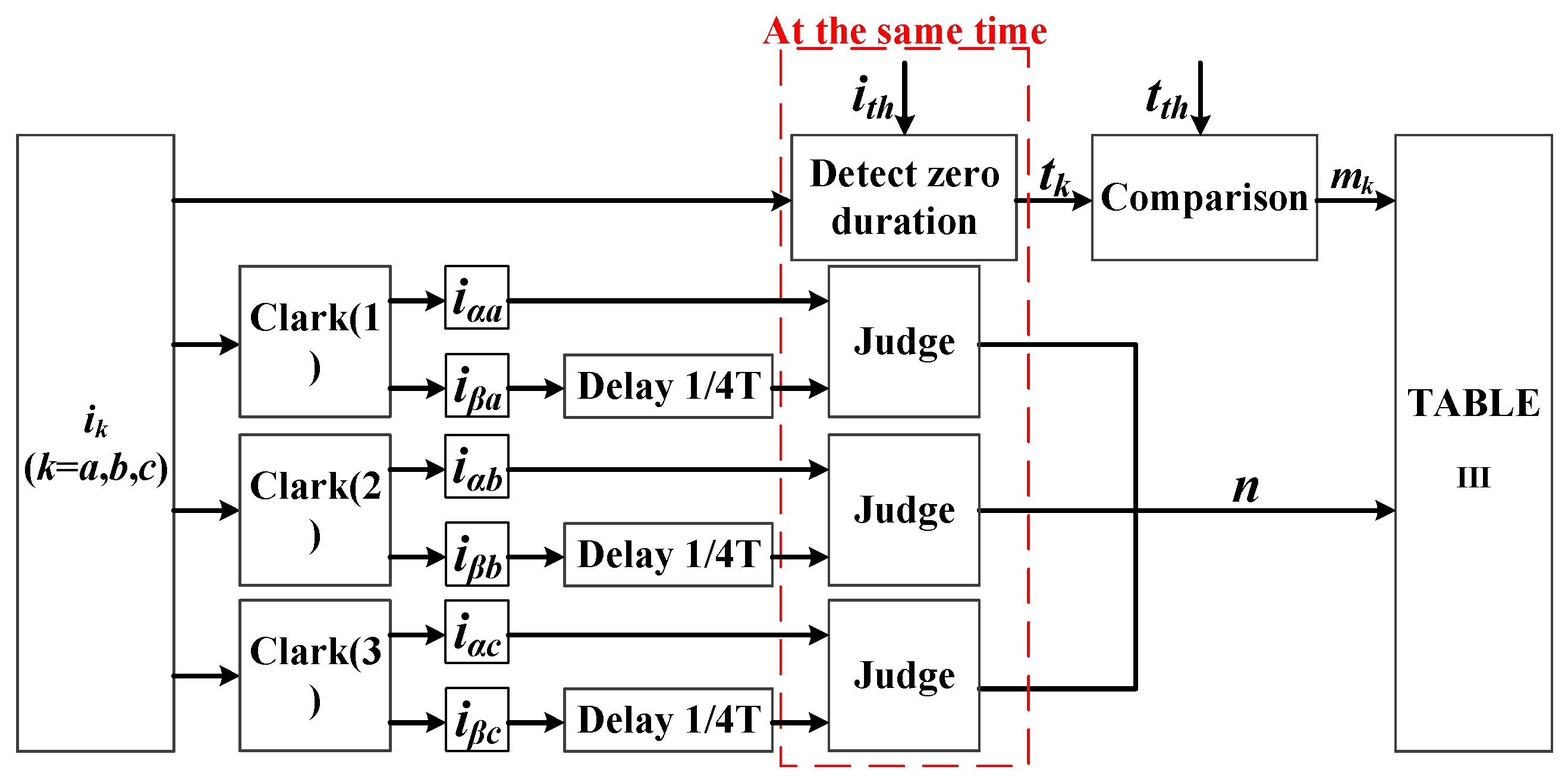
Figure 3 shows a block diagram of the single open-switch fault identification system proposed in this article. The diagram includes two parts: the input current fault identification and the missed diagnosis detection. The input current fault identification can locate fault-leg and fault-side. Fault-leg location is determined through the zero-plateau in fault-leg currents. The fault-leg is located where the duration t_k of the zero-plateau in the k-leg zero current is greater than its threshold tth. The fault-side is located based on reconstruction variables i_βa, i_βb, and i_βc obtained through Clark transformation and 0.25 T phase shifting (T is the period of the AC power grid).

The relationship between single open-switch faults and the flag bits for fault identification are shown in

Table 3. Relationship between single open-switch faults and flag bits.

Fault Switch	Flag Bits
	ma	mb	mc	n
None	0	0	0	0
Ma1	1	0	0	1
Ma2	1	0	0	0
Mb1	0	1	0	1
Mb2	0	1	0	0
Mc1	0	0	1	1
Mc2	0	0	1	0

. The flag bit m_k of the faulty leg and flag bit n of the faulty switch are both Boolean variables. When m_k = 1, the fault is located at leg k. When n = 1, the fault is in the up-leg and when n = 0, the fault is in the low-leg.

It is possible to miss a diagnosis when the modulation ratio is too small. Therefore, carrying out the missed diagnosis detection by harmonic analysis is necessary. When the detection result is inconsistent with the fault identification result, the time threshold will adjust automatically.

3.2. Fault-Leg Location of Single Open-Switch Faults

When a single open-switch fault occurs in a Vienna rectifier, the duration t_k of the zero-plateau in the fault-leg current lasts longer than the duration of zero-crossing in the non-faulty leg currents. Thus, the duration of zero-value can be used to locate the faulty leg. Electromagnetic interference, current harmonics, detection errors, and other factors make the fault-leg current fluctuate around zero during operations. Therefore, it is necessary to define a diagnostic threshold ith to help determine if input current is zero.

The zero-current flag bit ε_k is defined as:

$${\epsilon }_k=\left\{\begin{array}{ll}\begin{array}{ll}1,& \left|i_k\right|<i_{th}\\ 0,& \left|i_k\right|\ge i_{th}\end{array},& k=a,b,c\end{array}\right.$$

(13)

where ε_k = 1 represents the k-leg current at zero-crossing or on the current platform, and ε_k = 0 represents the current at another value state.

When ε_k = 1, the trigger counter W_k (k = a, b, c) begins counting. The duration of the counting is T_p. During counting, W_k is incremented by 1 when ε_k = 1 and remains the same when ε_k = 0. W_k is cleared when the counter enters sleep state. The duration t_k of zero-current is given as:

$$\begin{array}{cc}{t}_k=W_k{T}_s,& k=a,b,c\end{array}$$

(14)

where T_s is the current sampling period.

The flag bit m_k for leg faults is defined as:

$$m_k=\left\{\begin{array}{ll}\begin{array}{ll}1,& t_k>t_{th}\\ 0,& t_k\le t_{th}\end{array},& k=a,b,c\end{array}\right.$$

(15)

where m_k = 1 indicates that the faulty switch is in leg k and m_k = 0 indicates leg k is fault-free.

Zero-current diagnostic threshold ith and zero-current time threshold tth affect the accuracy of fault-leg location. Based on three-leg AC input currents from simulation and real-world experiments, the recommended values for the diagnostic threshold ith and time threshold tth were about 5% peak current and 0.08 T, respectively.

3.3. Fault-Side Location of Single Open-Switch Faults

When an open-switch fault occurs at the up-leg, the zero-plateau appears in the positive half cycle and when the fault occurs in the low-leg, the zero-plateau appears in the negative half cycle. Given the difficulty of calculating with the x-y coordinate system, the input current was subjected to Clark transformation and the α-β coordinate system was used to locate the fault side. To make comparison convenient, the reconstruction variable i_β is delayed by 0.25 T.

Clark transformation is carried on [i_a, i_b, i_c]^T, [i_b, i_c, i_a]^T, and [i_c, i_a, i_b]^T to construct variables [i_αa, i_αb, i_αc]^T and [i_βa, i_βb, i_βc]^T, which indicate the fault-side, and these variables are expressed as:

$$\left[\begin{array}{c}{i}_{\alpha a}(t)\\ i_{\alpha b}(t)\\ i_{\alpha c}(t)\end{array}\right]={\displaystyle \frac{2}{3}}\left[\begin{array}{ccc}1& -{\displaystyle \frac{1}{2}}& -{\displaystyle \frac{1}{2}}\end{array}\right]\left[\begin{array}{ccc}{i}_a(t)& i_b(t)& i_c(t)\\ i_b(t)& i_c(t)& i_a(t)\\ i_c(t)& i_a(t)& i_b(t)\end{array}\right]$$

(16)

$$\left[\begin{array}{c}{i}_{\beta a}(t)\\ i_{\beta b}(t)\\ i_{\beta c}(t)\end{array}\right]={\displaystyle \frac{2}{3}}\left[\begin{array}{ccc}0& {\displaystyle \frac{\sqrt{3}}{2}}& -{\displaystyle \frac{\sqrt{3}}{2}}\end{array}\right]\left[\begin{array}{ccc}{i}_a(t^{\prime })& i_b(t^{\prime })& i_c(t^{\prime })\\ i_b(t^{\prime })& i_c(t^{\prime })& i_a(t^{\prime })\\ i_c(t^{\prime })& i_a(t^{\prime })& i_b(t^{\prime })\end{array}\right]$$

(17)

where t′ = t − 0.25 T and t had sampling points within 0.08 T.

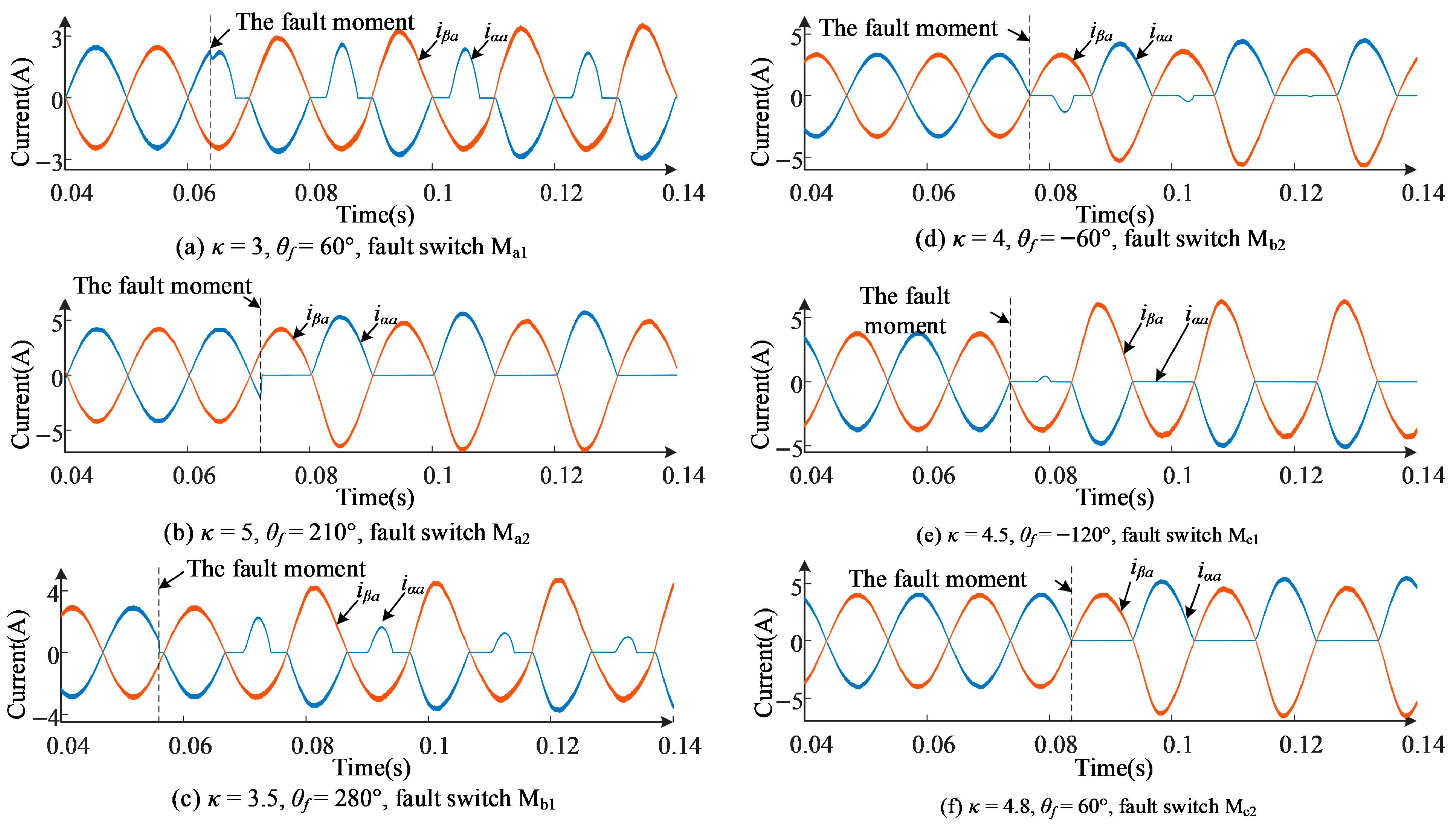
Using the system in Figure 3, some simulation results of i_αk and i_βk are shown in Figure 4.

The following conclusions can be drawn from the results in Figure 4:

(1)

Under normal operation, the waveform shows that if i_β is delayed by 0.25 T, i_α and i_β have equal frequency and amplitude, but a phase difference of 180°.

(2)

When k-leg single open-switch fault occurs, the zero-plateaus of i_αk and i_k appear or disappear simultaneously. The duration of either plateau is equal to each other.

(3)

During the zero-plateau in i_αk, i_βk is negative when the fault is in the up-leg and positive when the fault is in the low-leg.

The grid frequency fluctuates around the power frequency so i_βk may not all be positive or negative when i_αk experiences a zero-plateau within 0.08 T.

The counters W_βk1 and W_βk2 were designed to be synchronized with the trigger counters W_k. When a zero-plateau occurs within 0.08 T, counter W_βk1 is incremented by 1 if i_βk is greater than zero, and counter W_βk2 is incremented if otherwise.

The flag bit n_k for every switch, and flag bit for n are defined as:

$$n_k=\left\{\begin{array}{ll}0,& W_{\beta k1}\ge W_{\beta k2}\\ 1,& W_{\beta k1}<W_{\beta k2}\end{array}\right.$$

(18)

$$n=n_a+n_b+n_c.$$

(19)

3.4. The Missed Diagnosis Detection of Single Open-Switch Faults

Compared with the input current identification, the missed diagnosis detection based on the output voltage is more reliable. The difference in capacitor voltage is decomposed by Fast Fourier transform and the amplitude A₀ of DC component is selected as the fault characteristic. The missed diagnosis flag F is defined as:

$$F=\left\{\begin{array}{ll}1,& A_0\ge A_{th}\\ 0,& A_0<A_{th}\end{array}\right.$$

(20)

The misdiagnosis can be avoided when the time threshold tth is amplified reasonably, but a large time threshold tth is easy to cause missed diagnosis if the boost ratio is too small. In order to ensure the rapidity of fault diagnosis, the input current fault identification should be faster than the missed diagnosis detection. When missed diagnosis flag F is 1 but the fault is not identified by current identification, the time threshold tth should reduce automatically reduced to ${t^{\prime }}_{th}$ until the fault bit m_k appears.

$${t^{\prime }}_{th}=t_{th}-0.025\kappa T$$

(21)

3.5. Harmonic Analysis and Comparative Perspective

The harmonic characteristics of the proposed diagnostic method warrant explicit analysis to clarify its operational principle and distinguish it from alternative approaches. The voltage-based verification stage specifically monitors the harmonic spectrum of the capacitor voltage difference (ΔU = u_C1 − u_C2). As established analytically in Section 2.3, a single open-switch fault produces a characteristic harmonic signature: a significant increase in the DC offset and the second harmonic component of ΔU, while higher-order harmonics remain relatively unchanged. This response constitutes a localized, topology-specific harmonic fingerprint that directly results from the fault-induced modification of the converter’s internal current paths.

This mechanism differs fundamentally from system-level harmonic impedance analysis, a well-established technique for grid disturbance detection. Impedance-based methods model the frequency-dependent relationship between harmonic voltages and currents at the grid interface to monitor overall power quality and identify disturbance sources in multi-converter systems. While highly effective for system-wide supervision, these methods generally exhibit slower response times due to the need for steady-state harmonic extraction, rely on accurate grid-side measurements, and typically identify disturbance zones rather than specific faulty components within individual converters.

The distinction delineates complementary roles in a hierarchical diagnostic framework. System-level impedance analysis provides a “top-down” macro-perspective on grid health and stability, ensuring compliance with standards such as IEEE 519 [19] and IEC 61000-3-6 [23]. Conversely, the proposed method offers a “bottom-up” micro-diagnosis that leverages internal converter signals for rapid, device-level fault identification. For applications demanding immediate response to prevent secondary damage or maintain power quality compliance, the exploitation of these immediate, internal harmonic signatures proves particularly advantageous. Consequently, these approaches can operate synergistically: impedance monitoring safeguards overall system integrity, while embedded diagnostic algorithms like the one proposed ensure the operational reliability of individual power electronic units.

4. Experimental Results

4.1. Verify the Effectiveness of the Fault Identification

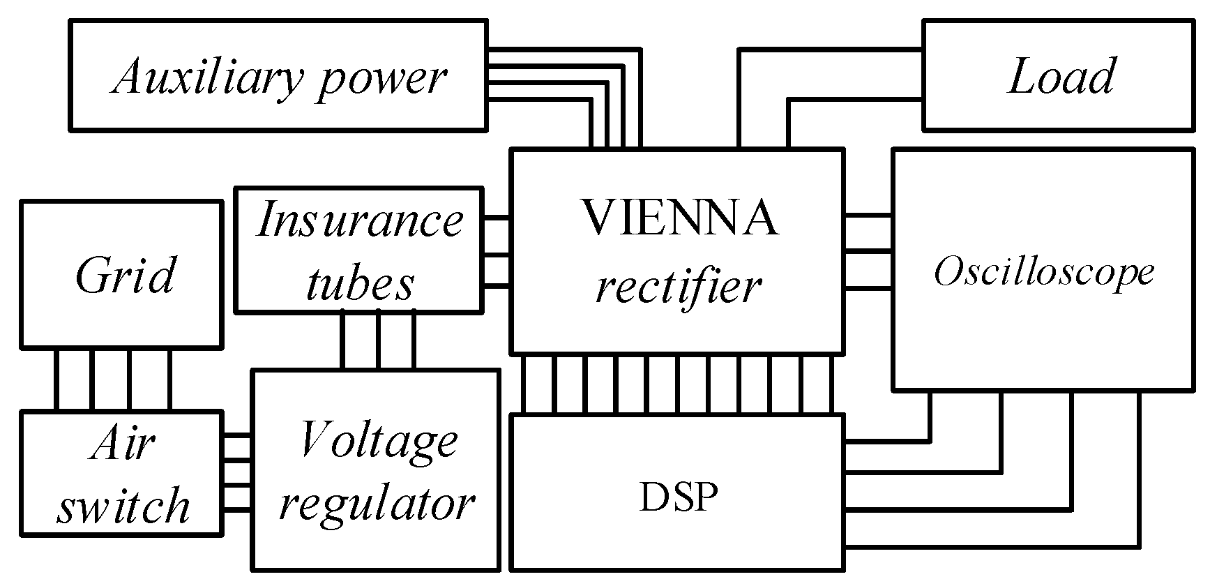
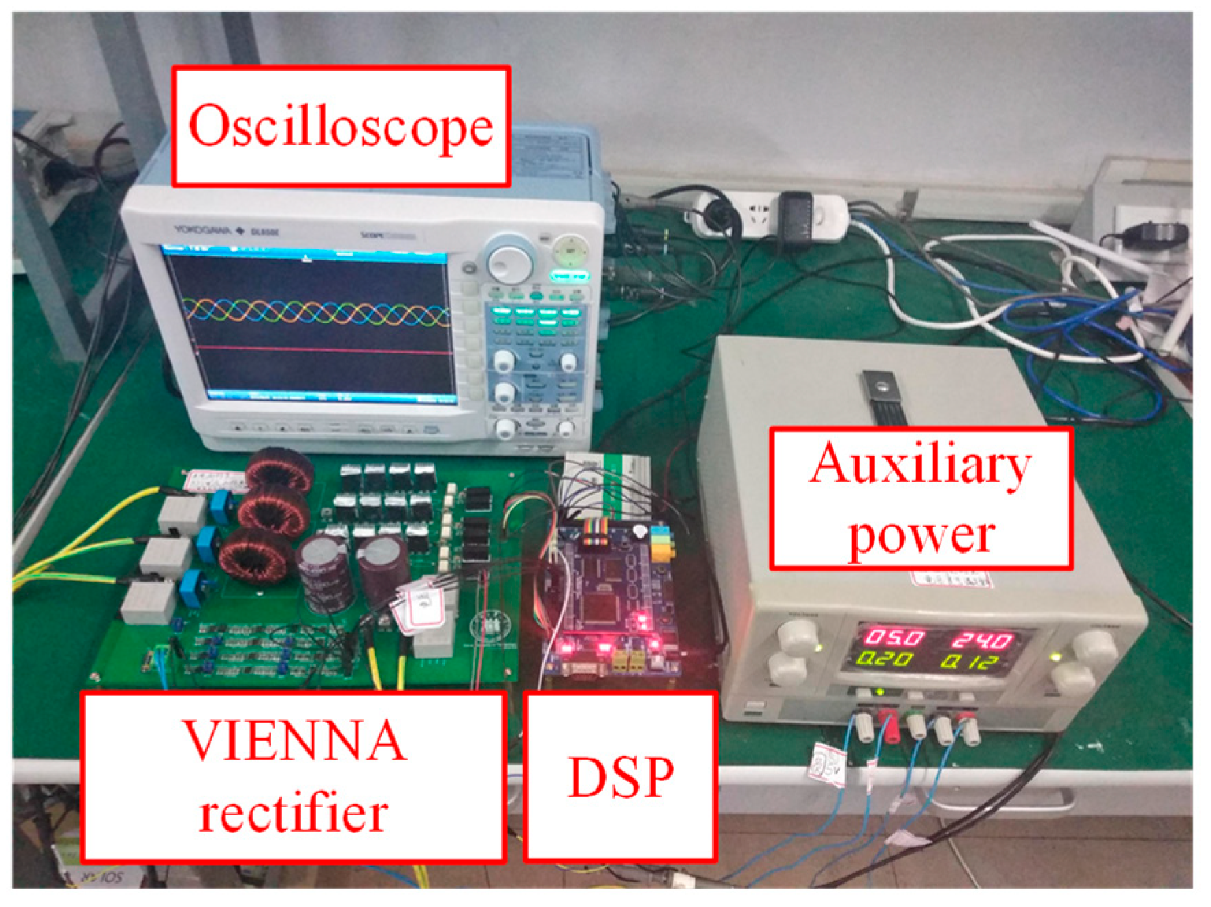
To verify the operation of the proposed fault identification method through real-world testing, an experimental platform was set up as seen in Figure 5 and Figure 6. The control part was realized by DSP TMS320F28335, and the test circuit parameters are shown in Table 3.

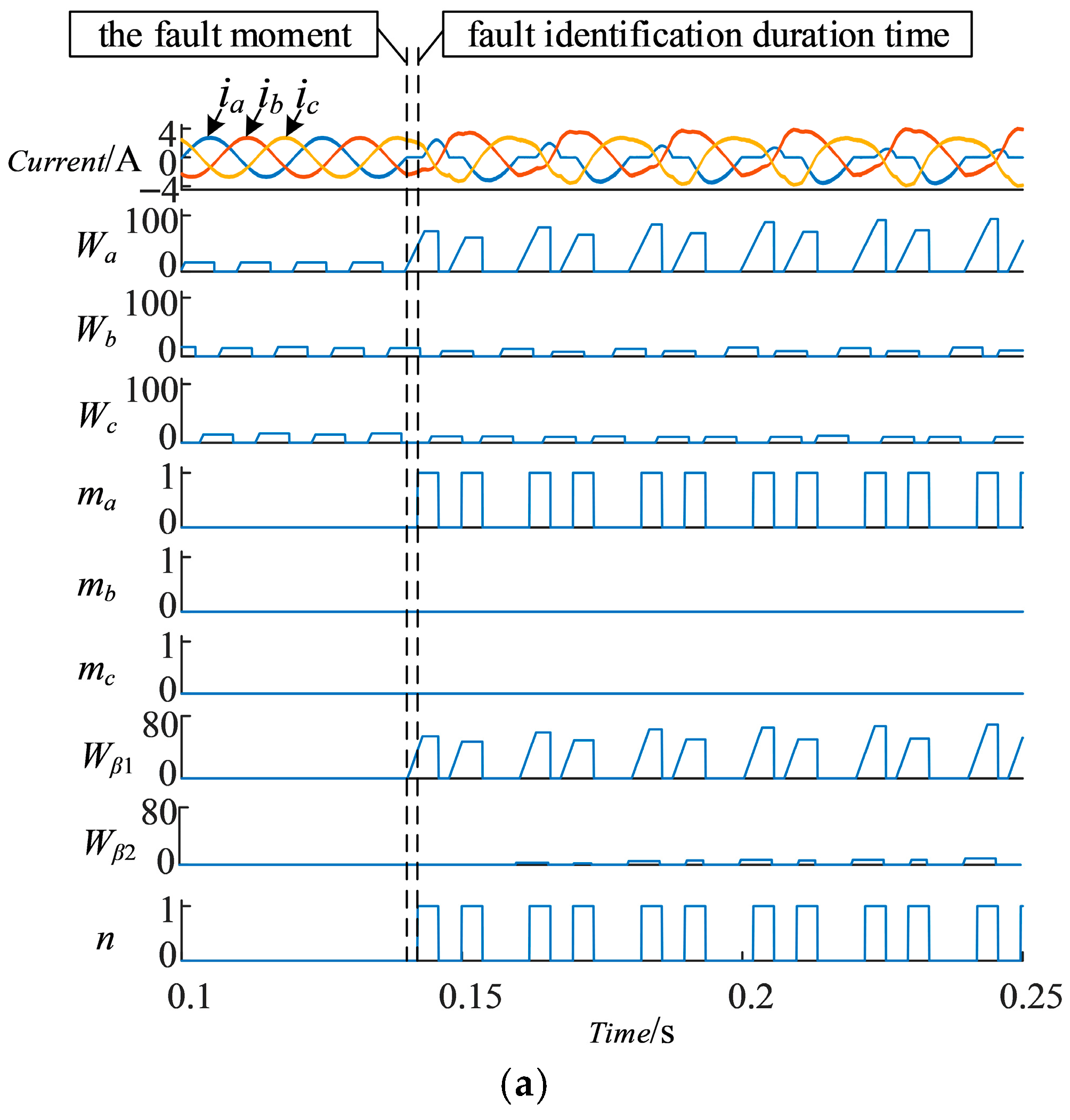
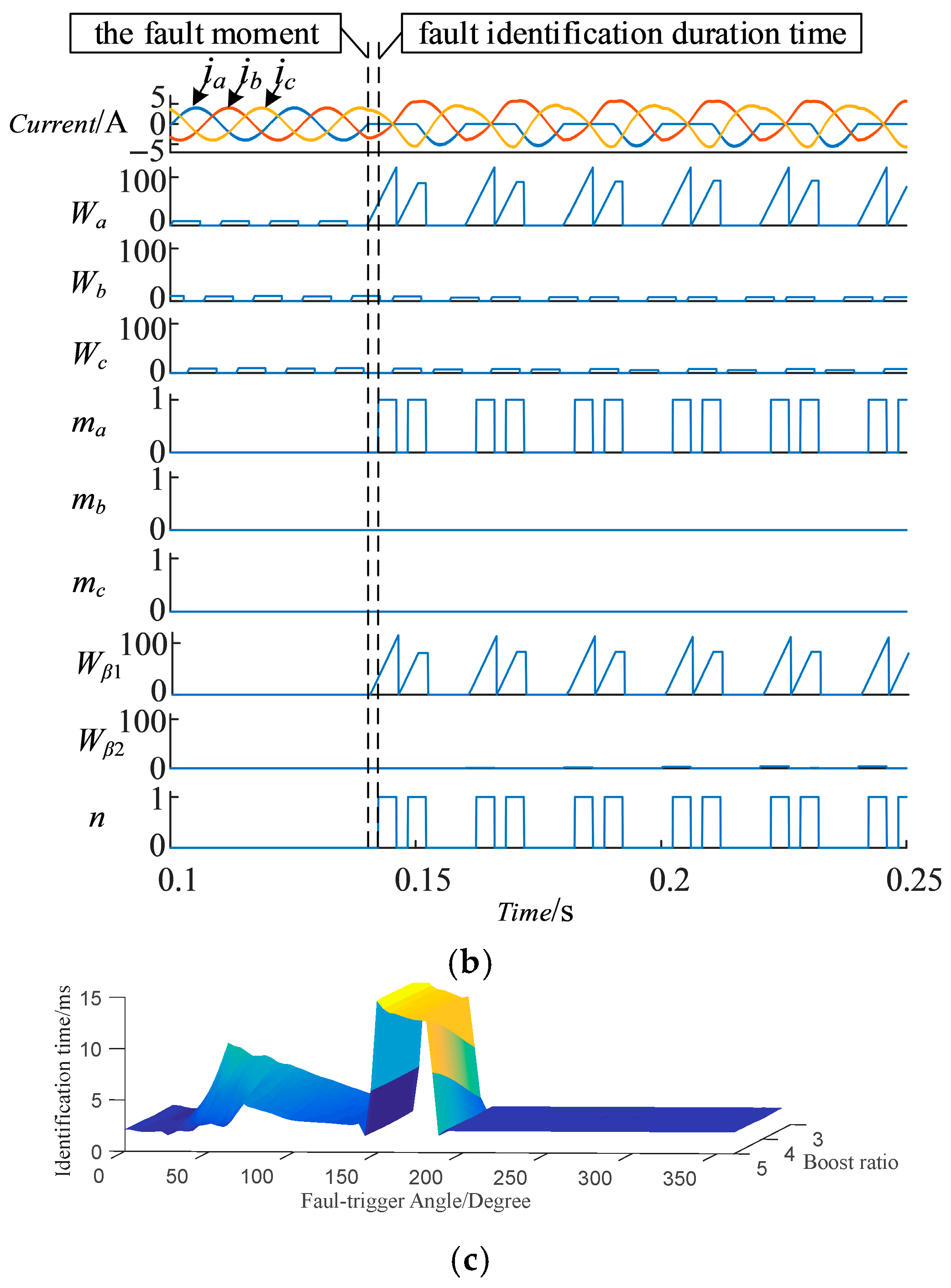
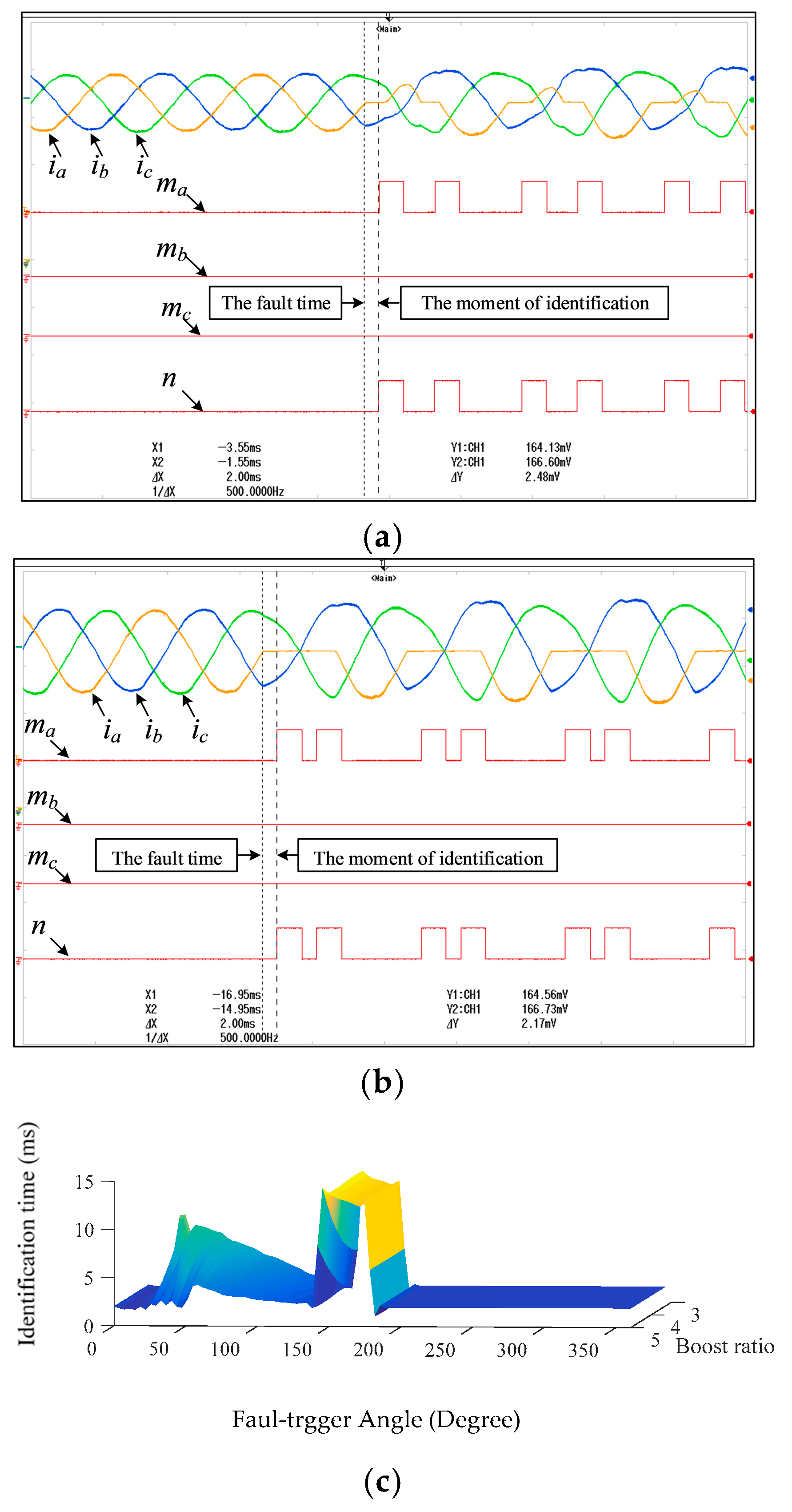
The boost ratio κ (3.3, 3.7, 4, 4.35, 4.57, 5) and fault-trigger angle (0°, 4.5°, 9° … 351°, 355.5°, 360°) were changed to verify the occurrence of single open-switch faults. Some of the simulation results are shown in Figure 7 and some of the results from the experiment are shown in Figure 8.

The simulation results in Figure 7 are consistent with the experiment results in Figure 8. The following conclusions are drawn from Figure 7 and Figure 8:

(1)

At the fault trigger point 0.1421 s, the first rising edge of the fault-leg location ma arrived regardless of whether the zero-plateau of the fault current had a peak. The same occurred with switch fault location n_a.

(2)

When the fault trigger angle θ_f was close to 180°, the duration of fault identification increased rapidly. This was because the duration of the zero-plateau was not long enough to trigger the rising edge of the fault-leg. Therefore, the zero-plateau could not be detected until the next zero-plateau arrived. The fault switch maintained open-circuit state during the half-cycle between both zero-plateaus.

(3)

The shortest durations of fault identification were 1.708 ms for simulation and 1.8 ms for real-world experiment. The longest durations for fault identification were 14.15 ms for simulation and 13.7 ms for real-world experiment. According to data from the real-world experiment, the duration of fault identification ranged from 9% T to 68.5% T of zero-plateaus.

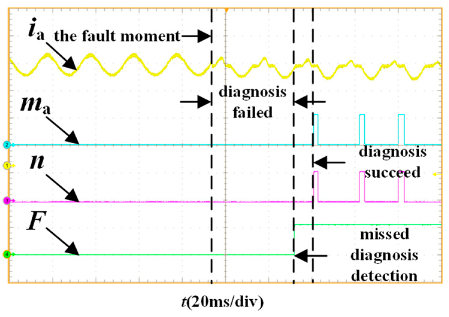
To verify the effectiveness of the missed diagnosis detection, an experiment was carried out, and the experiment result are shown in Figure 9. The missed diagnosis detection can detect the fault when the current identification method has missed diagnoses. The missed diagnosis flag F is set to 1 and the time threshold is automatically reduced. After about 8 ms, the current fault identification acts correctly.

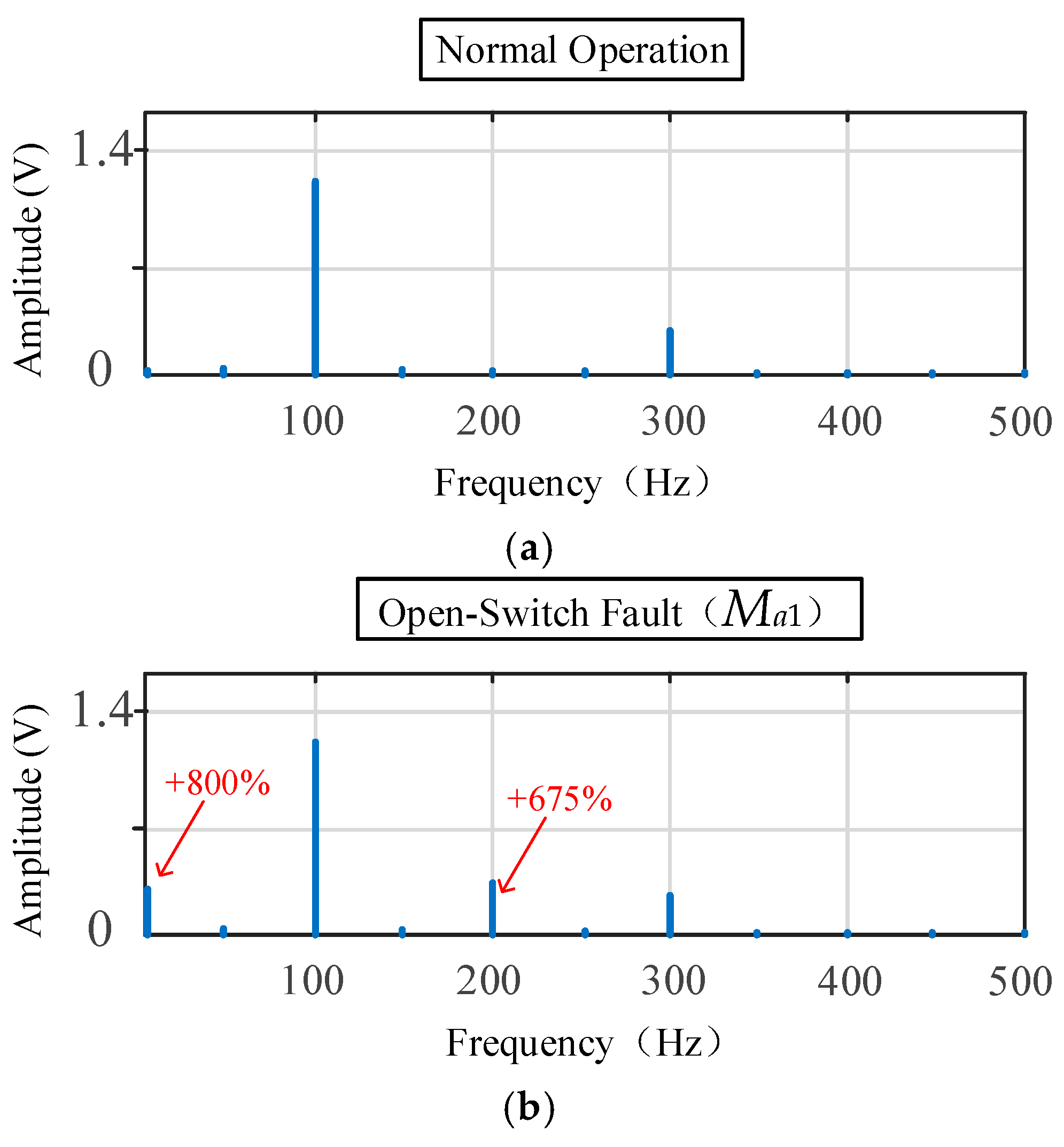
To validate the harmonic analysis presented in Section 2.3, the harmonic spectrum of the capacitor voltage difference ΔU (u_C1 − u_C2) was measured experimentally. Figure 10a shows the FFT analysis under normal operation, dominated by the 100 Hz component. Following an open-switch fault at M_a1, Figure 10b demonstrates the characteristic harmonic shift predicted theoretically: the DC component increases from 0.02 V to 0.18 V (800% rise), and the 200 Hz component increases from 0.04 V to 0.31 V (675% rise). These measurable changes confirm the reliability of the voltage-based verification stage in the proposed diagnostic system.

4.2. Robustness Verification

Table 4. Performance comparison of fault diagnosis methods.

Method	Avg. Diagnosis Time	Hardware Requirement	Computational Load	Valid M Range
Normalized Current [10]	>10 ms	Standard sensors	Low	M > 0.5
Vector Trajectory [13]	8–15 ms	Voltage sensors may be needed	Medium	M > 0.4
AI-Based [15]	5–20 ms	Standard sensors + computing	High	Full range
Proposed Method	2.5 ms	Standard sensors only	Low	M > 0.3

compares the performance of the proposed method with existing diagnostic approaches. The proposed method achieves an average diagnosis time of 2.5 ms, significantly faster than conventional methods (8–15 ms) while requiring no additional hardware. It maintains effectiveness across a wide modulation range (M > 0.3) and exhibits low computational complexity suitable for real-time implementation in standard digital controllers.

In order to verify the robustness of the proposed fault identification method, experiments were carried out under grid power interference and load mutation. The results show that the proposed fault identification method has good robustness.

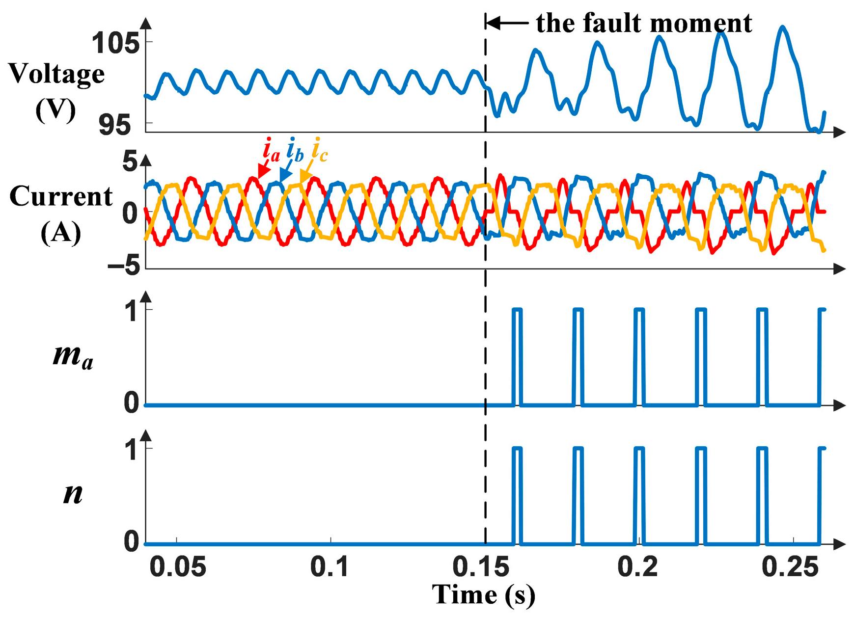
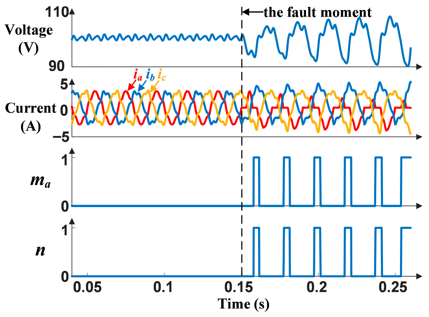
Figure 11 shows the simulation results of fault diagnosis system under three-phase voltage unbalance condition, including the waveforms of output voltage, input current, a-phase fault flag bit and upper leg fault flag bit. The voltage unbalance condition is u_A = 1.2u_B = 1.2u_C and the unbalance degree is far beyond the power quality standards specified in IEEE Std 112-1991 [24], IEEE Std 1159-1995 [25], IEC 61000 [26] and GB/T14549-93 [27]. The output voltage fluctuated before 0.15 s. At 0.15 s, the switch M_a1 experiences an open-switch fault, and the fault flag bits m_a and n are set to 1. The fault identification method can still act accurately even though the three-phase voltage is unbalanced.

Figure 12 shows the simulation results of fault diagnosis system when the input voltage has large harmonics. In this simulation, each phase contains 10% fifth harmonic and 5% seventh harmonic, which far exceeds the power quality standard of IEEE, IEC, and GB. The input current has obvious distortion before 0.15 s. At 0.15 s, Ma₁ has an open-switch fault, and the fault flag bits ma and n are set to 1. The fault identification method can still act accurately even though the input voltage has large harmonics.

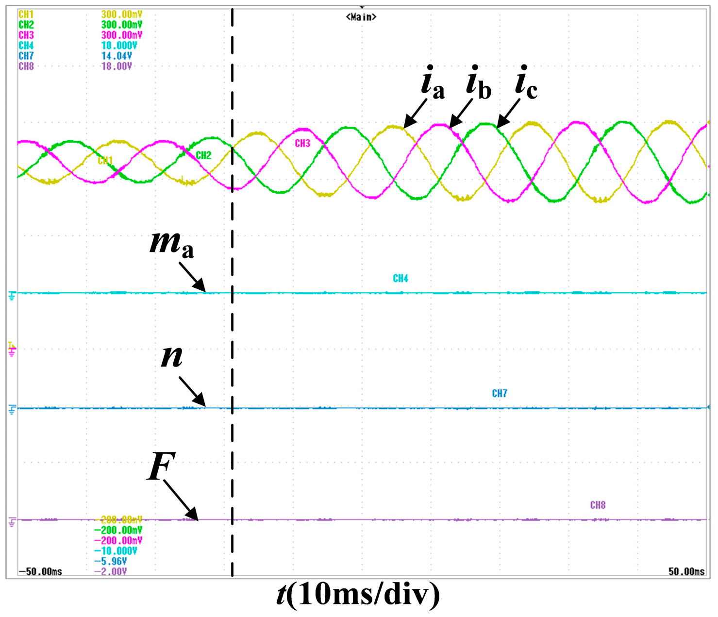
Figure 13 shows the experimental results when the load changes from 100 Ω to 50 Ω. It can be seen from the results that there will be no misdiagnosis when the load changes.

4.3. Summary and Correlation Analysis

The experimental results demonstrate strong consistency between theoretical predictions and practical measurements. The harmonic signatures of ΔU (Figure 3) align with the analytical derivations in Section 2.3, while the current-based fault identification times (1.8–13.7 ms) match simulation predictions within practical tolerances. The proposed two-stage diagnostic architecture effectively combines the speed of current feature extraction with the reliability of voltage harmonic verification, as evidenced by the successful operation of the missed-diagnosis detection mechanism (Figure 9). This integrated approach ensures robust performance across various operating conditions, including challenging low-modulation-ratio scenarios.

5. Conclusions

This study presents a fast and reliable diagnostic method for single open-switch faults in three-phase Vienna rectifiers. The proposed two-stage approach combines instantaneous current analysis and capacitor voltage harmonic monitoring to achieve accurate fault identification with minimal latency and no additional hardware.

The first stage identifies faulted legs by detecting characteristic zero-current plateaus in input phases, enabling diagnosis within one-sixth of a grid cycle. The second stage verifies this identification by analyzing harmonic components of DC-link capacitor voltage differences, providing adaptive threshold adjustment to prevent missed detections under challenging conditions. Experimental validation demonstrates the method’s effectiveness across various operating scenarios, including different fault locations, modulation ratios, and load conditions. The approach shows robust performance against grid disturbances while maintaining computational efficiency suitable for real-time implementation in standard digital controllers.

Beyond technical performance, the proposed method addresses practical industrial needs. Its rapid diagnostic capability (1.8–13.7 ms) enables timely intervention to prevent prolonged operation with distorted currents that could violate grid harmonic standards such as IEEE 519 [24]. This positions the method as an enabler for predictive maintenance strategies, contrasting with conventional protection schemes that often lead to unscheduled downtime. The algorithm’s simplicity and compatibility with standard digital signal processors facilitate cost-effective industrial implementation, enhancing both system reliability and grid-friendly operation.

While validated for the specific three-leg Vienna rectifier topology in this study, the method’s applicability to alternative converter configurations requires further investigation. Future research directions include: (1) extending the algorithm to four-switch and modular Vienna rectifier variants, (2) developing integrated fault-tolerant control strategies based on the diagnostic outputs, and (3) optimizing performance for boundary conditions through enhanced feature extraction techniques. Exploration of the method’s integration with system-level harmonic monitoring frameworks also presents a promising direction for comprehensive power quality management.

References

1. Dutta, S.; Bauman, J. An Overview of 800 V Passenger Electric Vehicle Onboard Chargers: Challenges, Topologies, and Control. IEEE Access 2024, 12, 105850–105864. [Google Scholar] [CrossRef]
2. Song, W.; Yang, Y.; Du, M.; Wheeler, P. Study of Constant DC-Voltage Control for VIENNA Rectifier Under No-Load Condition. IEEE Trans. Transp. Electrif. 2025, 11, 4730–4743. [Google Scholar] [CrossRef]
3. Lee, J.-S.; Lee, K.-B. Carrier-Based Discontinuous PWM Method for Vienna Rectifiers. IEEE Trans. Power Electron. 2015, 30, 2896–2900. [Google Scholar] [CrossRef]
4. Ali, A.; Khan, M.M.; Yuning, J.; Ali, Y.; Faiz, M.T.; Chuanwen, J. ZVS/ZCS Vienna rectifier topology for high power applications. IET Power Electron. 2019, 12, 1285–1294. [Google Scholar] [CrossRef]
5. Cheng, H.; Ma, Y.; Wang, C. A Modified One Cycle Control of VIENNA Rectifier for Neutral Point Voltage Balancing Control Based on Cycle-by-cycle Correction. In 2018 IEEE International Power Electronics and Application Conference and Exposition (PEAC); IEEE: New York, NY, USA, 2018. [Google Scholar]
6. Tian, S.; Campos-Gaona, D.; Mortazavizadeh, S.; Peña-Alzola, R.; Anaya-Lara, O. Low Harmonics Offshore Hybrid HVDC System Based on Vienna Rectifier and Voltage Source Converter with Back-up Capability. IEEE Trans. Energy Convers. 2024, 39, 2169–2183. [Google Scholar] [CrossRef]
7. Yang, S.; Xiang, D.; Bryant, A.; Mawby, P.; Ran, L.; Tavner, P. Condition Monitoring for Device Reliability in Power Electronic Converters: A Review. IEEE Trans. Power Electron. 2010, 25, 2734–2752. [Google Scholar] [CrossRef]
8. Smet, V.; Forest, F.; Huselstein, J.-J.; Richardeau, F.; Khatir, Z.; Lefebvre, S.; Berkani, M. Ageing and Failure Modes of IGBT Modules in High-Temperature Power Cycling. IEEE Trans. Ind. Electron. 2011, 58, 4931–4941. [Google Scholar] [CrossRef]
9. Fuchs, F.W. Some diagnosis methods for voltage source inverters in variable speed drives with induction machines—A survey. In Proceedings of the 29th Annual Conference of the IEEE Industrial Electronics Society (IEEE Cat. No.03CH37468), IECON′03, Roanoke, VA, USA, 2–6 November 2003; Volume 2, pp. 1378–1385. [Google Scholar]
10. Shi, T.; He, Y.; Deng, F.; Tong, J.; Wang, T.; Shi, L. Online diagnostic method of open-switch faults in PWM voltage source rectifier based on instantaneous AC current distortion. IET Electr. Power Appl. 2018, 12, 447–454. [Google Scholar] [CrossRef]
11. Estima, J.O.; Cardoso, A.J.M. A new approach for real-time multiple open-circuit fault diagnosis in voltage source inverters. In Proceedings of the 2010 IEEE Energy Conversion Congress and Exposition, Atlanta, GA, USA, 12–16 September 2010; pp. 4328–4335. [Google Scholar]
12. Qiu, Y.; Jiang, H.; Feng, Y.; Cao, M.; Zhao, Y. A New Fault Diagnosis Algorithm for PMSG Wind Turbine Power Converters under Variable Wind Speed Conditions. Energies 2016, 9, 548. [Google Scholar] [CrossRef]
13. Sleszynski, W.; Nieznanski, J.; Cichowski, A. Open-Transistor Fault Diagnostics in Voltage-Source Inverters by Analyzing the Load Currents. IEEE Trans. Ind. Electron. 2009, 56, 4681–4688. [Google Scholar] [CrossRef]
14. Jung, J.-H.; Ku, H.-K.; Son, Y.-D.; Kim, J.-M. Open-Switch Fault Diagnosis Algorithm and Tolerant Control Method of the Three-Phase Three-Level NPC Active Rectifier. Energies 2019, 12, 2495. [Google Scholar] [CrossRef]
15. An, Y.; Sun, X.; Ren, B.; Zhang, X. Open-Circuit Fault Diagnosis for a Modular Multilevel Converter Based on Hybrid Machine Learning. IEEE Access 2024, 12, 61529–61541. [Google Scholar] [CrossRef]
16. Xia, Y.; Xu, Y.; Zhou, N. A Transferrable and Noise-Tolerant Data-Driven Method for Open-Circuit Fault Diagnosis of Multiple Inverters in a Microgrid. IEEE Trans. Ind. Electron. 2024, 71, 8017–8027. [Google Scholar] [CrossRef]
17. Hu, X.; Hu, J.; Guan, Q.; Zhang, Y.; Wang, Q.; Zhou, D. An Open-Circuit Fault Diagnosis Method for Charging Piles Based on Attention Mechanism. In Proceedings of the IECON 2024—50th Annual Conference of the IEEE Industrial Electronics Society, Chicago, IL, USA, 3–6 November 2024; pp. 1–6. [Google Scholar]
18. Deng, Y.; Jia, H.; Lian, G.; Wang, X.; Liu, Y. Switch Open-Circuit Fault Diagnosis of the Vienna Rectifier Using the Transformer–BiTCN Network with Improved Snow Geese Algorithm Optimization. Electronics 2025, 14, 3655. [Google Scholar] [CrossRef]
19. IEEE 519-2022; IEEE Standard for Harmonic Control in Electric Power Systems. IEEE Standard Association: Piscataway, NJ, USA, 2022.
20. Lai, Y.; Sun, Y.; Shan, P.; Ge, J.; Wang, T.; Li, Y. An Active Suppression Method for Harmonic Current Based on Grid-Forming Converter in Distorted Grids; Proceedings of the CSEE; CSEE: Beijing, China, 2026; pp. 1–12. Available online: https://link.cnki.net/urlid/11.2107.tm.20250416.1734.019 (accessed on 24 December 2025).
21. Ma, Y.; Han, S.; Wang, Z.; Li, R.; Zhao, S. Study on oscillation characteristics and dynamic interaction of control link of a VSC-HVDC connected direct drive wind farm. Trans. China Electrotech. Soc. 2025, 20250460. [Google Scholar] [CrossRef]
22. Lee, J.-S.; Lee, K.-B. Open-Switch Fault Diagnosis and Tolerant Control Methods for a Vienna Rectifier Using Bi-Directional Switches. In Proceedings of the 2018 IEEE Energy Conversion Congress and Exposition (ECCE), Portland, OR, USA, 23–27 September 2018; pp. 4129–4134. [Google Scholar]
23. IEC TR 61000-3-6:2008; Electromagnetic Compatibility (EMC)—Part 3-6: Limits-Assessment of Emission Limits for the Connection of Distorting Installations to MV, HV and EHV Power Systems. International Electrotechnical Commission: Lodon, UK, 2008.
24. IEEE Std 112-1991; IEEE Standard Test Procedure for Polyphase Induction Motors and Generators. IEEE Standard Association: Piscataway, NJ, USA, 1991.
25. IEEE Std 1159-1995; IEEE Recommended Practice for Monitoring Electric Power Quality. IEEE Standard Association: Piscataway, NJ, USA, 1995.
26. IEC 61000-2-2:2002; Electromagnetic Compatibility (EMC)—Part 2-2: Environment—Compatibility Levels for Low-Frequency Conducted Disturbances and Signalling in Public Low-Voltage Power Supply Systems. IEC: Geneva, Switzerland, 2002.
27. GB/T14549-93; Quality of Electric Energy Supply Harmonics in Public Supply Network. The National Standards of the People’s Republic of China: Beijing, China, 1993.
Figure 1. Topology of a three-leg Vienna rectifier.
Eng 07 00060 g001
Figure 2. The three-leg input currents and voltages of the two balance capacitors before and after open-switch fault.
Eng 07 00060 g002
Figure 3. Block diagram of the proposed fault identification system.
Eng 07 00060 g003
Figure 4. The construction variables iaa and iβα with 0.25 T delay after single open-switch fault occurs.
Eng 07 00060 g004
Figure 5. Block diagram of platform for experiment.
Eng 07 00060 g005
Figure 6. Physical diagram of platform for experiment.
Eng 07 00060 g006
Figure 7. Some simulation results of three-leg input currents, fault-location, and duration of fault identification. (a) ik, mk, and n before and after Ma1 experienced single open-switch fault. κ = 3.30 and θf = 0°; (b) ik, Wβk, mk, and n before and after Ma1 experienced single open-switch fault. κ = 4.76 and θf = 0°; (c) Duration of fault identification under different boost ratios and fault trigger angles.
Eng 07 00060 g007aEng 07 00060 g007b
Figure 8. Some experimental results of three-leg input currents, fault-location, and duration of fault identification. (a) ik, mk, and n before and after Ma1 experienced single open-switch fault. κ = 3.30 and θf = 0°; (b) ik, Wβk, mk, and n before and after Ma1 experienced single open-switch fault. κ = 4.76 and θf = 0°; (c) Duration of fault identification under different boost ratios and fault trigger angles.
Eng 07 00060 g008
Figure 9. The experimental results of the missed diagnosis detection when the diagnosis is missed.
Eng 07 00060 g009
Figure 10. Harmonic spectrum of capacitor voltage difference ΔU under (a) normal and (b) fault conditions. (a) Normal Operation (M = 0.8); (b) Open-Switch Fault (Ma1, M = 0.8).
Eng 07 00060 g010
Figure 11. The simulation result of the robustness of fault diagnosis under unbalanced three-phase voltages.
Eng 07 00060 g011
Figure 12. The simulation result of the robustness of fault diagnosis under voltage harmonic interference.
Eng 07 00060 g012
Figure 13. The experimental verification result of the robustness of fault diagnosis under sudden load changes.
Eng 07 00060 g013