Review

Review of Watershed Hydrology and Mathematical Models

by
Shiblu Sarker
1,* and
Olkeba Tolessa Leta
2
1
Dam Safety and Floodplains, Virginia Department of Conservation and Recreation, Richmond, VA 23219, USA
2
Bureau of Groundwater Modeling and Assessment, St. Johns River Water Management District, Palatka, FL 32178, USA
*
Author to whom correspondence should be addressed.
Eng 2025, 6(6), 129; https://doi.org/10.3390/eng6060129
Submission received: 30 April 2025 / Revised: 9 June 2025 / Accepted: 15 June 2025 / Published: 17 June 2025
(This article belongs to the Section Chemical, Civil and Environmental Engineering)

Abstract

:
This study provides a comprehensive overview of watershed hydrology and mathematical models, focusing on its hydrological features and the implementation of hydrological modeling for effective water resource modeling and assessment, planning, and management. The study presents a thorough review of the primary transport mechanisms of water within a watershed, particularly the river network, and examines its physical and stochastic characteristics. It also discusses the derivation of governing equations for various hydrological processes within a watershed, including evaluating their applicability in the context of watershed modeling. Additionally, this research reviews the generation of hydrologic flux from rainfall events within a watershed and its subsequent routing through overland flow and channel networks. Furthermore, the study examines commonly utilized statistical distributions and methods in watershed hydrology, emphasizing their implications for watershed modeling. Finally, this research evaluates various mathematical models used in watershed processes modeling, highlighting their respective advantages and disadvantages in the context of water resource management studies.

1. Introduction

1.1. The Development of Hydrology

Hydrology originated from ancient Greek thinkers such as Homer (about 1000 B.C.), Thales, Plato, and Aristotle, as well as Roman philosophers like Lucretius, Seneca, and Pliny and scholars from the medieval period, and refers to the study of the hydrologic cycle and water movement [1]. Despite limited supporting evidence, Anaxagoras of Clazomenae (Ancient Greece 500 to 428 B.C.) postulated that solar radiation evaporates seawater into the atmosphere, resulting in the formation of precipitation, and then underground reservoirs can be used to preserve river currents by collecting rainwater [1]. Theophrastus (Ancient Greece 372 to 287 B.C.) improved the concept of the hydrologic cycle, which involves the movement of water in the atmosphere and the formation of precipitation through condensation and freezing. An engineer from the Roman era, Marcus Vitruvius, who lived around the time of Christ, also postulated that groundwater originates from the infiltration of rain and snow, based on his examination of Theophrastus’ works. People in Ancient China also documented many weather-related phenomena, such as rain, sleet, snow, and wind, and the utilization of rain gauges dates back to around 1000 B.C. The concept of the hydrologic cycle was initially formulated in China around 900 B.C., in India around 400 B.C., and in Persia around the ninth century. This revolutionized the field of hydrology by shifting its focus from a philosophical approach to an observational one. Leonardo da Vinci (1452–1519) was the first person who observed and studied the stream velocity distribution. He accurately measured the disparities between the velocities of the water’s surface and bottom in a cross-sectional area using a weighted rod and animal bladder at various locations of a stream and quantified the distribution of stream velocity [1]. He also observed that the flow velocity of a stream increases at the surface due to contact with the air, which has a lower density than water and generates reduced drag, and the water beneath is in direct contact with the soil, which is stationary and possesses a greater weight than water. According to Frazier (1974), Leonardo wrote more extensively about hydraulics than any others [1]. Bernard Pilissy (French, 1510 to 1589) demonstrated that rivers and springs originate from precipitation. Pierre Perrault (French, 17th century) showed quantitatively that runoff is only a small fraction of total rainfall. He accurately recognized that rainfall is a main factor contributing to runoff and deduced that the remainder of it was lost due to transpiration, evaporation, and diversion. The field of hydraulic measurements and experiments made significant progress during the 18th century [2]. Bernoulli’s and Chezy’s formulas and equations were derived, and better instruments, such as a tipping-bucket rain gauge and a current meter, were also invented. The field of hydrology made significant progress during the 19th century [1]. In 1802, Dalton first proposed the concept of evaporation [3]. In 1839, Hagen Poiseuille established a precise definition for capillary flow [2,4]. Finally, in 1850, Mulvaney developed a systematic method for determining peak flood flows [1,5]. The principles of Darcy’s law, Rippl’s storage diagram, and Manning’s open-channel flow formula were established in 1856, 1883, and 1891, respectively [1,2,6,7,8]. The field of quantitative hydrology was in its early stages of development throughout the early 1900s. Empirical methodologies tackled hydrological concerns. Hydrologists transitioned progressively from relying on observational evidence to employing logical data analysis [1]. For example, Green and Ampt (1911) formulated a physical model to calculate infiltration [9], Hazen (1914) investigated flood peaks and water storage, Richards (1931) developed an equation for unsaturated flow [10], Sherman (1932) developed a unit hydrograph technique [11], Horton (1945) established the theory of infiltration and drainage basins [12], and Gumbel (1958) proposed the extreme value law [1,13]. Due to advances in technologies and progressive understanding of the concept of hydrology over time, computers have revolutionized hydrology, facilitating extensive research on a broad scale, similar to their impact on other sciences. Computer simulations utilize intricate hydrologic theories and summary data to enhance comprehension and facilitate planning. For instance, recent developments in electronics and data transformation enable the accurate prediction of floods in real time and the retrieval of data from distantly recording devices. Programming facilitates computational tasks for hydrologists. Enhanced comprehension and methodologies in hydrology lead to more precise and comprehensive hydrological solutions. Hydrologic problems have a significant impact on the lives of several individuals, including ecosystem functioning and life-sustaining functions.

1.2. Watershed Hydrology

A watershed, also called a drainage basin, constitutes a land area that aggregates water from precipitation, snowmelt, surface runoff, and subsurface flows and channels it towards a river, lake, or ocean [14]. The demarcation of its boundaries and the modulation of water flow are governed by topographical features such as ridges, hills, and mountains. A complex hydrological network of streams and rivers undertakes the collection and conveyance of water, where smaller tributaries coalesce with larger ones, ultimately forming the primary river and exiting the basin [15]. A thorough comprehension of watersheds is imperative for evaluating water availability, managing flood risks, and maintaining ecosystem health [15,16]. These systems underpin diverse species and serve as essential ecological units [17]. The health of ecosystems within a watershed is contingent upon water availability and quality, as well as hydrological and geomorphic processes [18,19].
Watershed hydrology examines the behavior of water within a watershed, a geographical area where precipitation collects and directs its flow towards a common outlet, such as a river, lake, or sea. This discipline is crucial for the management of water resources, flood prediction, and the evaluation of water availability [18]. Watershed hydrology mainly focuses on the concept of the hydrologic cycle that encompasses precipitation, evapotranspiration ( E T ), infiltration, groundwater recharge, surface runoff, interflow, groundwater or base flow, and streamflow, including water quality. Additionally, watershed hydrology involves floodplain mapping and flood risk assessment that are indispensable [1,14]. Water evaporates from water bodies evaporation process and bare surfaces and transpires from vegetation through transpiration process, collectively called evapotranspiration. The Evapo-transpired water eventually returns to the ground as precipitation (see Figure 1). Historical meteorological data is instrumental in monitoring precipitation, estimating water resources, and comprehending the system’s inflows. Accurate measurement of E T rates is vital for estimating water loss and availability. Precipitation either infiltrates into the soil or becomes surface runoff. Assessing infiltration and soil moisture conditions is necessary to determine soil water content and its absorption capacity. A comprehensive understanding of surface runoff, interflow, and baseflow is essential for predicting streamflow and formulating water management strategies. Monitoring streamflow is fundamental for watershed hydrology. Hydrologists collect streamflow data, analyze flow patterns, and investigate the impacts of environmental changes, such as land use/land cover and climate changes, and other anthropogenic activities. The assessment of water quality that focuses on nutrients, sediments, water contaminants, and other pollutants is critical in ensuring ecosystem health and the usability of water. Anthropogenic activities such as deforestation, urbanization, and agricultural practices exert a significant influence on watershed hydrology and ecology, modifying water flow and quality. To reduce negative effects and guarantee the sustainable use of water resources, effective water planning and management strategies are crucial. To implement effective water resources planning and management strategies, researchers, water resources managers, and decision-makers need to have a clear understanding of hydrological processes and behaviors at a given scale, such as the watershed level. As measuring the different hydrological processes (shown in Figure 1) at the watershed scale is impractical, utilizing sophisticated computer tools such as models is very useful. However, the applicability of models generally depends on the watershed characteristics and size, the availability and quality of data, and the representation of each hydrological process using mathematical equations. Therefore, the main objective of this review is to provide a detailed understanding of watershed hydrology, concepts, and processes, as well as provide recommendations on when and where to use the available hydrologic and hydraulic models.

2. Watershed Hydrologic Processes

Hydrologic processes encompass different natural occurrences that dictate how water moves and is distributed within a watershed or drainage area. Comprehending hydrologic processes is crucial for water resource management, flood prediction and mapping, and preserving ecological harmony. Below are some significant hydrologic processes within a watershed.
Precipitation serves as a crucial water source for a watershed and involves the transformation of atmospheric water vapor into a liquid or solid form that falls to Earth’s surface in the form of rain, snow, sleet, or hail. Various forms of precipitation are identified, including rain (2.5–7.5 mm/h), snow (made up of ice crystals), drizzle (small droplets with a diameter of 0.5 mm and an intensity of 1 mm/h), glaze (rain that freezes upon impact), sleet (small, clear ice pellets), and hail (ice balls larger than 8 mm). The device used to gather and measure precipitation on the ground surface is called a rain gauge. There are two main types of rain gauges: non-recording gauges, such as Symon’s gauge, and recording gauges, such as tipping-bucket, weighing-bucket, and natural-siphon types [1]. Due to advancements in technology and science, precipitation can also be measured remotely by using satellites [20,21]. When the precipitation rate exceeds the soil’s infiltration rate and water capacity, surface runoff occurs, causing excess water to flow over the land surface into streams, rivers, and other water bodies. The infiltration rate, an important metric, is typically measured with infiltrometers, which mimic rainfall to gauge the rate at which water penetrates the soil. Changes in soil moisture over time are tracked using soil moisture sensors. Measuring precipitation interception by plants is particularly difficult, but methods like throughfall measurements are used, where water captured by vegetation is collected as it drips off leaves [1].
Surface runoff, which represents the flow of water on the land surface, is affected by various factors, such as the soil type, land use, and slope. Surface runoff occurs when the infiltration rate of the soil is smaller than the rainfall rate or when the soil is saturated. The infiltration process involves the entry of water from the land surface into the soil, with the rate depending on soil characteristics, land cover, and the initial moisture content of the soil [1].
Evapotranspiration, the process where liquid water becomes water vapor due to solar energy and heat, happens from water bodies, plants, and damp soil surfaces. Transpiration, the release of water vapor from plant leaves and stems, is crucial to the water cycle, similar to a plant’s breathing process [1]. The evaporation process that happens when water evaporates from water bodies or bare surfaces is usually measured using evaporation pans or lysimeters. Whereas large-scale transpiration measurement is complex, sap flow sensors and porometers have been commonly used to estimate transpiration rates in plants at certain locations. The combination of evaporation and transportation processes forms evapotranspiration (ET). Condensation is indirectly inferred through humidity levels measured by instruments like hygrometers [1]. The transport of water vapor in the atmosphere is studied by using weather balloons equipped with radiosondes and other devices to measure temperature, humidity, and pressure at different altitudes. The deposition of water vapor as ice crystals or snowflakes is not often measured directly, but snow gauges measure the depth and water content of snow on the ground [1].
Streamflow refers to the sum of surface runoff, interflow, and baseflow components of streams or rivers. Stream gauges, commonly used tools, measure water flow in rivers and streams, providing data on the volume of water passing a specific point over time. The lateral movement of water through underground soil and rock layers, known as subsurface or interflow, is difficult to measure directly. Groundwater levels and flow are monitored with wells and piezometers, and then techniques like dye tracing help study water movement through the subsurface. This subsurface flow plays a crucial role in the hydrological dynamics of a watershed. Groundwater or baseflow represents the portion of streamflow derived from groundwater discharge, sustaining river or streamflow during dry spells and ensuring water quality [1]. Groundwater, originating from water infiltrating through soil layers, accumulates in underground aquifers, moving slowly through the subsurface, and it influences streamflow, especially during the dry periods [1].
Hydrological models can help to simulate these hydrologic processes using a precipitation, terrain, or digital elevation model ( D E M ), land use/land cover, and soil data to predict streamflow, flooding events, and water availability. This research underpins the development of sustainable water management strategies, optimizing water allocation for agricultural, potable, and industrial uses while considering environmental impacts and climate change [14]. This comprehensive approach involves meticulous data collection, in-depth analysis, sophisticated modeling, and strategic development.

3. River Networks: Primary Transport Features of Watershed
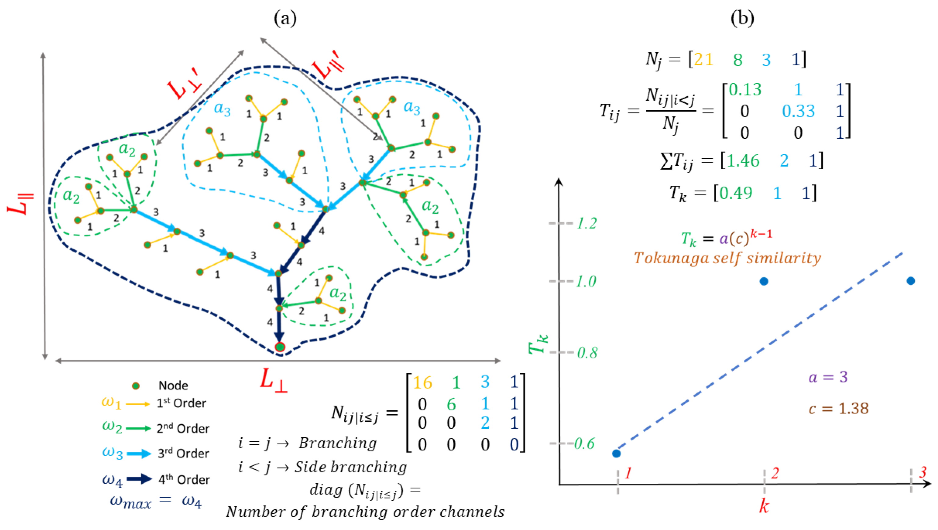
The river network ( R N ) within a watershed describes the interconnected system of rivers, streams, and waterways that traverse a specific watershed or drainage basin. The R N in a given watershed comprises multiple streams and rivers that originate from various sources within the watershed and eventually merge into larger water bodies. A thorough understanding of the R N within a given watershed is crucial for effective water resource management, assessing potential flooding risks, maintaining water quality, and sustaining the ecological balance in aquatic ecosystems [15,16]. Streams and rivers exhibit a hierarchical structure within the broader R N . First-order streams combine to form second-order streams, which then merge to create third-order streams, and so on. This hierarchical arrangement reflects the natural movement of water from higher elevations to lower elevations, ultimately converging into the main discharge river or water body within the watershed. Streams and rivers are formed due to precipitation and various water sources flowing downward. As these hydrological features receive inflow from smaller streams, they merge and increase in size. Ultimately, all the water within a specific watershed disperses into a single discharge point, such as the mouth of a river or a lake.
R N scaling rules relate to the observed empirical relationships and patterns in the shapes and features of river systems at different scales. The study of scaling laws has been a significant focus within geomorphology, a field dedicated to understanding the physical processes that shape the Earth’s surface. The concepts and principles of scaling reveal the inherent patterns and connections within R N s. Nevertheless, it is important to recognize that these rules are empirical estimates and may not universally apply to all R N s. Various factors such as geology, climate, tectonics, and human activities can affect river systems’ behavior, potentially causing deviations from these scaling laws in certain instances. Below are some key scaling laws and concepts associated with R N s.
Basin allometry investigates the relationship between the size (area, volume) of a watershed or basin and its shape. This involves analyzing the mathematical connections between these properties. A basin may be characterized at any given location on a landscape, encompassing multiple sub-basins within each basin. Figure 2 shows hypothetical river basins with a longitudinal length of L and a characteristic width of L , along with sub-basins. Consequently, the area A of this basin is related to these dimensions by A L L , where L L b . Thus, A L 1 + b . These relationships are known as scaling laws, which explain how one dimension varies in proportion to another, as well as how the total area changes in relation to a particular length. Additionally, b = 1 represents geometric similarity or self-similarity, while b 1 is referred to as allometric scaling [22]. Several scaling laws link these quantities, with one of the most recognized being Hack’s law [23]. It describes the relationship between the length of stream segments and their drainage area (catchment area); i.e., l scales with A as l A h , where l is the main stream length and h is often called Hack’s exponent. A key aspect of Hack’s law is that h 1 / 2 [23]. The exponent h generally ranges from 0.5 to 0.7 and can vary based on geological and climatic conditions. Further comparisons of drainage basins of different sizes yield scaling in terms of L and L , such as A L n , l L d , and L L b .
Stream ordering is an essential method in R N analysis. It allows for logical comparisons between different network components and provides a basic language for describing network structure [24,25,26]. Horton first introduced stream ordering in his pioneering work on erosion [12], and Strahler later refined this method [27], leading to what is now known as Horton–Strahler stream ordering [28]. Melton describes this stream ordering most intuitively as an iterative pruning of a tree representing the network [29]. Generally, when a stream segment of order ω 1 joins with a stream segment of order ω 2 , the resulting stream will have an order of ω , where ω = max ( ω 1 , ω 2 ) + δ ω 1 , ω 2 . In other words, the stream order increases only when two segments of the same order merge; otherwise, the highest order is retained by the outflowing stream (see Figure 2). Conversely, Shreve proposed a method for classifying streams within an R N based on their hierarchy [30]. The smallest unbranched streams are first-order, and when two first-order streams converge, they form a second-order stream, and so forth. This system helps explain the hierarchical organization of R N s.
Horton’s Laws explain the statistical distribution of stream lengths within an R N [12]. The first law asserts that in a random R N , the number of streams of a specific order (branches of a certain size) is inversely proportional to their length, i.e., R n = n ω n ω + 1 . This R n is referred to as the bifurcation ratio. In other words, R n represents the ratio of the number of downstream channels to the number of upstream channels at a branching point in an R N . It provides insights into the branching structure of R N s. The second law states that the average length of streams of a particular order increases with the order, i.e., R l = l ¯ ω + 1 l ¯ ω . This R l is known as the stream length ratio. The third law indicates that the ratio of the drainage areas of the upstream channel order to those of the immediate downstream channel order remains constant for a given basin, i.e., R a = a ¯ ω + 1 a ¯ ω .
Figure 2. Horton–Strahler stream ordering of a hypothetical river basin, along with its R N (a) and the corresponding Tokunaga’s law (b); different colors indicate different orders (see details in [31]).
Eng 06 00129 g002
Tokunaga’s law pertains to a collection of ratios originally established by Tokunaga [32,33,34] and represents the average number of streams of order ω i flowing into a stream of order ω j as side tributaries. In this case of a ‘structurally self-similar network’, we can consider N i j to denote the number of streams of order i that are laterally connected to streams of order j when i j . The branching ratios can thus be described through an ( ω m a x 1 ) ( ω m a x 1 ) upper triangular square matrix T , where ω m a x is the maximum order of the basin. The elements of T are defined as T i j = N i j N j , where N j represents the total number of streams of order j. Tokunaga [33] suggested that, on average, the branching ratio T i j is independent of link orders i and j and depends only on their difference, k = j i . By defining T k = 1 n k i = 1 n k T i , i + k , where n k = ω m a x k represents the number of elements on the kth diagonal of T , a stronger condition for the self-similarity of side branching is defined as the ratio of two successive T k , being on average independent of k, i.e., T k + 1 T k = c [35]. Therefore, c is a fixed constant for a given RN, and Tokunaga’s ratios can be specified by two parameters, a and c, as T k = a ( c ) k 1 . This identity is commonly known as Tokunaga’s law (see Figure 2).
In addition to the previously described scaling law, area discharge scaling explores the relationship between the size of a river’s drainage basin and the average discharge (water flow) of that river. Larger drainage basins tend to have higher average discharges as a result of the accumulation of water from a larger area. This relationship can be described by various empirical equations or relationships, such as the rational method, regional regression equations, or power-law scaling. A common empirical relationship used to estimate the average annual discharge ( Q ) based on the drainage basin area ( A ) is a power-law equation. It is often represented as Q A ϵ , where ϵ is the scaling exponent that characterizes this relationship. Furthermore, research has shown that R N s tend to exhibit a fractal-like structure, meaning that their patterns repeat at different scales (see [36]). Fractal dimensions can be used to quantify the complexity of R N s, reflecting their self-similar patterns (see [36]).
R N s also play a significant role in watershed delineation from a digital elevation model ( D E M ), an essential step in watershed modeling. To do this, D E M high-resolution data can be obtained from a variety of sources. After removing inconsistencies, such as data gaps, surges, and sinks, D8 or D-infinity algorithms can be used to calculate the DEM flow direction. The accumulation of flow can then be calculated to identify stream networks. Setting a threshold value above which cells are deemed to be part of the stream network is a common method. Then, connections between adjacent cells in the stream network are typically made to form continuous stream segments. The watersheds can then be delineated by tracing the flow paths from the outlet locations (typically user-defined) upstream to the highest points on the flow accumulation grid. Various algorithms, such as the D-infinity method and the D8 method, can be utilized to complete this procedure. The watershed boundaries can then be refined by considering topographic features, such as ridges and valleys, that may influence flow patterns. Frequently, this stage requires manual editing or additional analysis.

4. Governing Equations for Water Cycle Phases on Watersheds

The aim of this section is to review the physical principles and governing equations that describe the stages of the hydrologic cycle within a watershed.
The Reynolds transport theorem ( R T T ) is a crucial principle extensively used in various branches of physics and engineering, including hydrology. This principle pertains to a mathematical framework that allows for the analysis of fluid flow properties within a specified region over time [1,37,38,39,40]. Named after Osborne Reynolds, a key figure in fluid dynamics, the R T T connects the rate of change in an extensive property (B), ( d B d t ) to the external factors causing this change. Mathematically, it can be expressed as
d B d t = d d t C V β ρ d V + C S β ρ V d A
To put it differently, Equation (1) indicates that the net rate of change in B equals the rate of change in B stored within the control volume ( C V ) plus the flux of B across the control surface ( C S ). This essential equation forms the foundation for all hydrological and watershed models. For instance, the mass balance equation can be derived using this principle [1,38,39,40]. If B represents mass (m), then the change in B will be zero, as mass (m) cannot be created or destroyed. Consequently, Equation (1) transforms as follows:
d B d t = 0 = d S d t + ( Q I )
Thus, the change in storage within a C V equals the inflow (I) minus the outflow (O), assuming constant density, which is commonly referred to as the continuity equation. Similarly, the energy balance can be derived from the R T T . According to the R T T , B can be expressed as B = E , where E represents the total energy in the system. This total energy is the sum of internal energy ( E u ), kinetic energy ( 1 2 m v 2 ), and potential energy ( m g z ), with z denoting elevation. Mathematically, this is written as E = E u + 1 2 m v 2 + m g z . Consequently, the intensive property can be expressed as
β = d B d m = d E d m = e u + 1 2 v 2 + g z
Here, e u represents the internal energy per unit mass. According to the first law of thermodynamics, the net rate of energy transfer into the system is equivalent to the rate at which heat is added to the system minus the rate at which the system performs work on its surroundings [1,37,38,39,40]. Mathematically, this is expressed as d B d t = d E d t = d H d t d W d t . Consequently, the energy equation can be formulated as follows:
d H d t d W d t = d d t C V e u + 1 2 v 2 + g z ρ d V + C S e u + 1 2 v 2 + g z ρ V d A
There are two primary forms of internal energy used in watershed modeling. Sensible heat refers to the portion of a system’s internal energy ( e u ) that varies with its temperature (T). As the temperature changes, the internal energy of the object changes proportionally, with the proportionality constant being the specific heat ( C p ), i.e., d e u = C p d T . The subscript p indicates that the specific heat is measured at constant pressure. Conversely, during a phase transition, such as when a substance changes from a solid to a liquid or a gas, it either absorbs or releases latent heat. The three significant latent heats are the heat of fusion for the transition from ice to water, the heat of vaporization for the transition from liquid water to water vapor, and the heat of sublimation for the direct transition from ice to water vapor.
When applying the R T T to the fluid momentum, B becomes m v , and β is d B d m = v . According to Newton’s second law, the rate of change in momentum over time corresponds to the net force exerted in a specific direction [1,37,38,39,40]. Hence, the R T T can be expressed as
F = d d t C V v ρ d V + C S v ρ V d A
This represents the integral form of the momentum equation for flows that are both unsteady and non-uniform. The practical application of Equation (5) can be easily illustrated in the context of open-channel flow, such as flow in a river or in a partially filled pipe [1,36,37,38,39,40,41]. In this scenario, three forces act on the C V : friction, gravity, and pressure. The pressure forces ( F p ) at the two ends of the C V section are equal and cancel each other out in uniform flow (i.e., y 1 = y 2 ). The friction force ( F f ) is the product of the wall shear stress τ 0 and the area over which it acts, P L , where P is the wetted perimeter of the cross-section, i.e., F f = τ 0 P L , with the negative sign indicating that the friction force opposes the flow direction. The weight of the fluid in the C V is γ A L , where γ is the specific weight of the fluid; thus, the gravity force ( F g ) is the component of the weight acting in the flow direction, given by F g = γ A L cos θ (see details in [1,2,37,38,39,40,42]). When θ is small, cos θ cos θ = S 0 , leading to the approximation τ 0 = γ A L S 0 P L = γ R S 0 . For steady uniform flow, S 0 = S f , so τ 0 = γ R S f . Therefore, using Equation (5), the conservation of momentum for a 1 D open-channel flow system (i.e., C V = x 2 x 1 ) without any lateral inflows can be expressed as
( γ A 1 y 1 γ A 2 y 2 ) x 1 x 2 γ A S f d x + x 1 x 2 γ A S 0 d x = d d t x 1 x 2 ρ Q d x + ρ Q 2 v 2 ρ Q 1 v 1
As in most practical cases, the density of water is constant, and since x 1 and x 2 are two arbitrary locations, we can write it in a differential form as follows:
d Q d t + d ( Q v ) d x + d ( g A y ) d x = g A ( S 0 S f )
Equation (7) is often referred to as the momentum equation in the longitudinal direction. Various types of flow, such as steady uniform flow (kinematic wave, i.e., S 0 = S f ), steady non-uniform flow (diffusive wave, which includes only the pressure term), steady dynamic flow (which includes both pressure and convective acceleration terms), and unsteady non-uniform flow (dynamic wave, which includes all terms), can be described using Equation (7) [1,2,37,38,39,40]. Equation (7) is applied in river and streamflow analysis, flood modeling, hydraulic structure design, sediment transport studies, erosion analysis, and open channel flow evaluation. Another well-known formula can be derived from Equation (7) under two assumptions: (a) steady uniform flow, where F g causing the flow is equal to F f , and (b) turbulent flow, where F f per unit wetted area is proportional to the square of the mean velocity. Thus, it can be expressed as follows:
F f = γ A L S f = k P L v 2
Equation (8) can be rearranged to give v = C R 1 / 2 S f 1 / 2 , where γ / k = C . This formula is commonly known as Chezy’s formula. Additionally, Darcy and Weisbach introduced a friction factor (f), primarily for pipe flow, which can be related to Chezy’s C as C = 8 g / f . Moreover, Manning’s equation can be derived from Chezy’s equation by setting C = R 1 / 6 n , where n is known as the Manning roughness. Manning’s equation is applicable for fully turbulent flow, while the Darcy–Weisbach friction factor (f) can be determined as a function of the Reynolds number R e and the relative roughness of the boundary [1,2,37,38,39,40,42]. On the other hand, the concept can also be applied to flow moving through a porous medium, which is an interconnected network of tiny conduits of various shapes and sizes. Assuming these tiny conduits are circular pipes with diameter D , under steady uniform flow, the wall shear stress is given by τ 0 = γ R S f = 8 μ v D , where μ is the dynamic viscosity of the fluid and R = D / 4 . Thus, mathematically, we can express it as follows:
v = γ D 2 32 μ S f
Equation (9) is known as the Hagen–Poiseulle formula for laminar flow in a circular conduit (i.e., pipe flow) [1,2,37,38,39,40]. In the case of a porous medium, the cross-sectional area A is partially occupied by soil or rock strata, so the ratio v = Q / A is defined as q, called the Darcy flux. Therefore, the flow in a porous medium is written as follows:
Q A = q = K S f
where K = γ D 2 32 μ represents the hydraulic conductivity of the medium, which depends on porosity ( η ), defined as the ratio of the volume of the voids to the total volume of the medium. Consequently, the actual mean velocity of the fluid in the medium is v a = q / η . Darcy’s law holds true as long as the flow remains laminar.
Besides momentum balance, energy balance is crucial for comprehending transport processes. Energy transport occurs via conduction, convection, and radiation. For instance, heat transfer happens through conduction, convection, and radiation. Conduction is driven by random molecular motion, where molecules at higher temperatures transfer energy to those at lower temperatures upon collision. In contrast, convection involves the bulk movement of a fluid, transferring heat energy through fluid stream eddy motion. Although convection operates on a larger scale than conduction in fluids, its effectiveness is influenced by fluid turbulence, leading to less precise characterization. Radiation, however, is the direct transfer of energy through electromagnetic waves and can occur even in a vacuum. The processes of conduction and convection that transfer heat energy also transport mass and momentum [1,37,38,39,40,43,44]. For each extensive property—mass, momentum, and energy—the rate of flow of the extensive property per unit area of the surface through which it passes is termed flux = flow rate area . For example, volumetric flux for any system can be expressed as q = Q A , the corresponding mass flux as m ˙ A = ρ Q A , the momentum flux as m ˙ V A = ρ Q V A = ρ V 2 , and the energy flux as d E d t A , where d E d t is the energy flow rate [1]. In conduction, the flux is directly proportional to the gradient of a potential. Fick’s law of diffusion ( f m = D d C d z ), Newton’s law of viscosity ( τ = μ d v d z ), and Fourier’s law of heat conduction ( f h = k d T d z ) are commonly used examples of conduction laws, where the mass ( f m ), momentum ( τ ), and energy ( f h ) fluxes are transported, respectively, with D, μ , and k known as the diffusion coefficient, viscosity, and thermal conductivity, respectively. In addition, C , v, and T denote concentration, velocity, and temperature, respectively. Convection transport involves turbulent eddies rather than individual molecular movement as in conduction. Conduction does not require fluid flow; however, convection does [1]. Similarly, the convective forms of extensive properties, that is, mass, momentum, and energy transport, may be modified as f m = ρ K w d C d z , τ = ρ K m d v d z , and f h = ρ C P K h d T d z , where the corresponding K w , K m , and K h are known as mass, momentum, and energy diffusivity L e n g t h 2 T i m e . It is noted that this transport in the direction of motion is known as advection and is described by the term C S β ρ V d A in Equation (1) [1,37,38,39,40,43,44]. To calculate the rates of momentum conduction and convection, it is necessary to understand the velocity distribution within the boundary layer. For air flowing over land or water, the logarithmic velocity profile is the appropriate model, where the velocity u is described as a function of the elevation z, as in Equation (11).
u u * = 1 κ ln z z 0
In this context, u * = τ 0 / ρ is referred to as the shear velocity. For open-channel flow, it is given by u * = g R S 0 . Here, z 0 represents the roughness height, and κ = 0.4 is known as the von Karman constant. Consequently, the velocity gradient in the transport equations can be substituted with u * κ z [1,37,38,39,40,43,44].
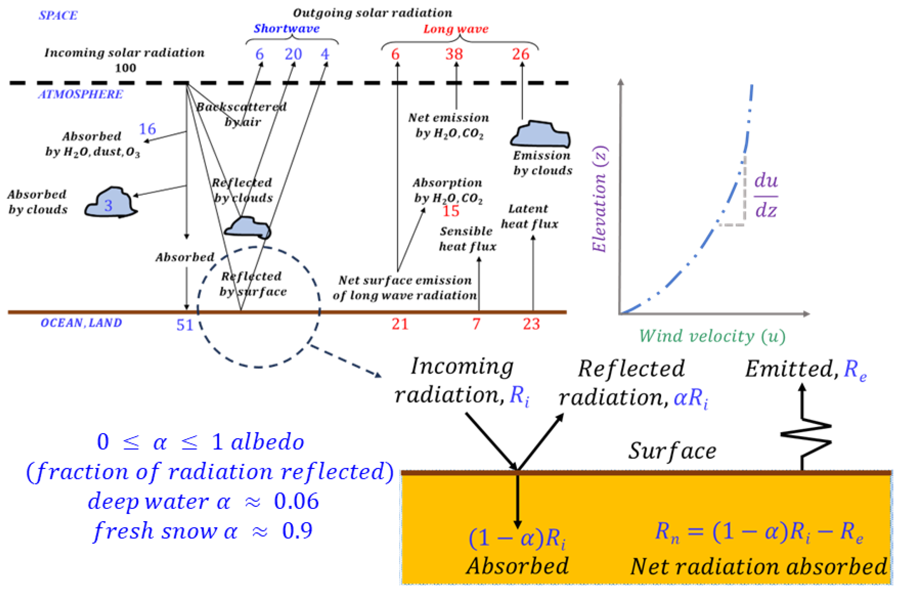
Furthermore, in terms of radiation, energy travels through electromagnetic waves, which can propagate even in a vacuum (see radiation balance in Figure 3). The rate of this transmission is affected by the surface temperature of the objects involved. The Stefan–Boltzmann equation provides a way of quantifying radiation, expressed as R e = E σ T 4 , where E is the surface emissivity, equal to one for a blackbody and 0.97 for water. The Stefan–Boltzmann constant is σ = 5.67 × 10 8 W/m2*K4. Wien’s wavelength is given by λ = 0.0029 / T meters, indicating that the Sun emits shorter wavelengths compared to the cooler Earth [1,14,37,38,39,40,43,44]. Atmospheric water exists largely in a gaseous state, but it can rapidly transition into a liquid or solid form through processes such as rainfall, water droplets, cloud formation, snowfall, hail, and ice crystal formation. The transport of gases in air through a hydrological system can be described by R T T [45,46,47,48,49,50,51,52,53,54,55], where B is the mass of water vapor. Therefore, intensive property β can be written as
β = d B d m = ρ v ρ a = q v
where ρ v and ρ a represent the densities of water vapor and moist air, respectively. Hence, the ratio of ρ v to ρ a is termed the specific humidity q v . The pressure of water vapor can be determined using Dalton’s law of partial pressures and the ideal gas law as e = ρ v R v T , where e denotes the pressure exerted by water vapor, R v is the gas constant, and T is the absolute temperature in ° K . Consequently, the partial pressure due to dry air can be expressed as p e = ρ d R d T , where p = ρ a R a T is the total pressure exerted by moist air. Given that ρ a = ρ d + ρ v and R v = R d / 0.622 , the specific humidity q v = 0.622 e p , where 0.622 represents the ratio of the molecular weight of water vapor compared to the mean molecular weight of dry air [1,45,46,47,48,49,50,52,54,55].
Air at a given air temperature can contain a maximum level of moisture, with the corresponding vapor pressure termed the saturation vapor pressure ( e s ). Relative humidity is defined as the quotient of the actual vapor pressure by its saturation vapor pressure at that specific temperature (i.e., R h = e / e s ), where the saturation vapor pressure ( e s ) as a function of temperature is
e s = 611 exp 17.27 T 237.3 + T
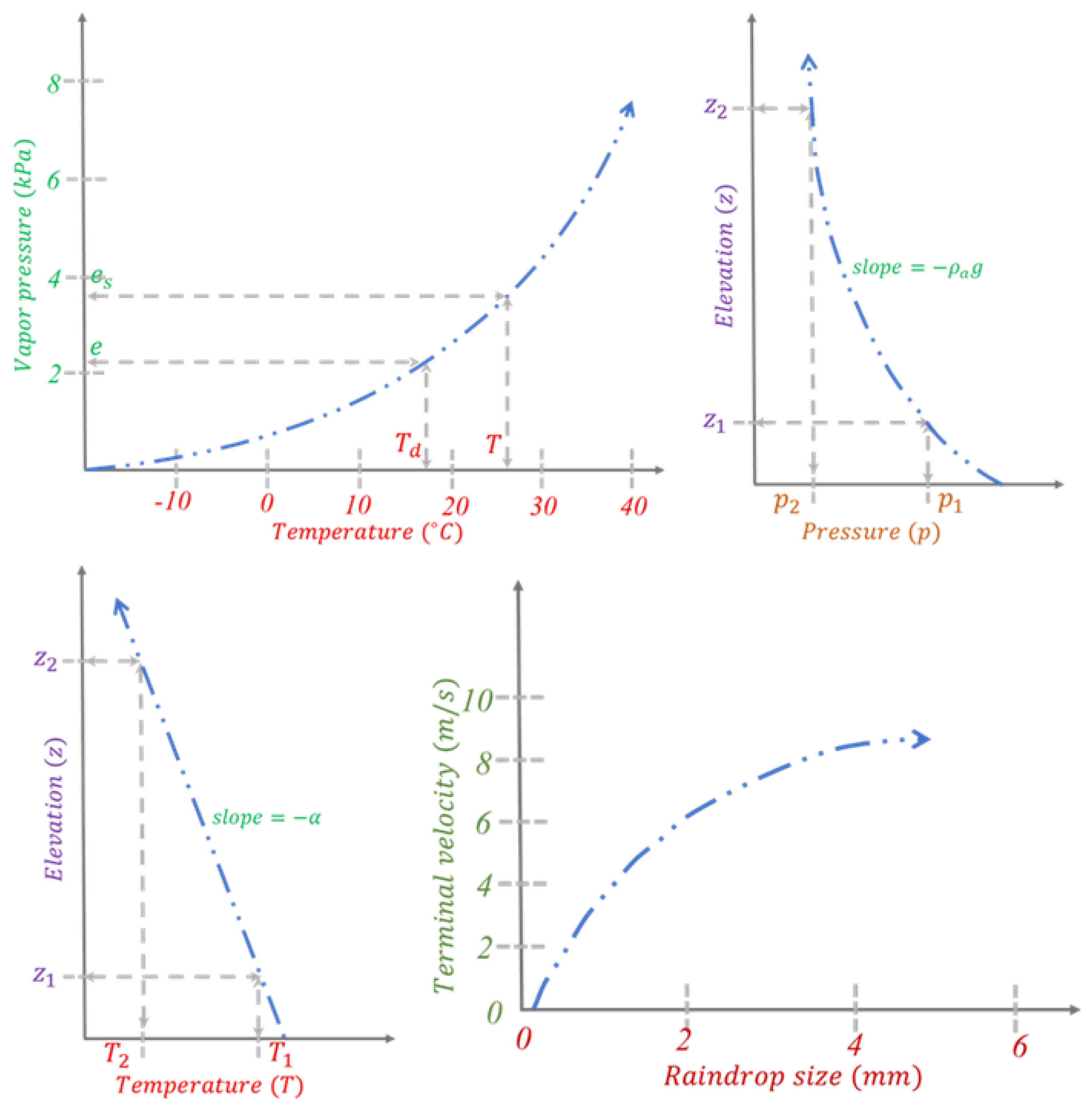
The temperature at which air becomes saturated at a specific humidity is referred to as the dew point temperature ( T d ). Furthermore, the hydrostatic pressure equation ( d p d z = ρ a g ) can be integrated with the ideal gas equation ( p = ρ a R a T ) to analyze the characteristics of water vapor in a stationary column. Furthermore, the change in air temperature with altitude is represented by d T d z = α . Consequently, a linear temperature change (see Figure 4), when combined with these two physical laws, results in a nonlinear pressure change (see Figure 4) with altitude as follows:
d p p = g α R a d T T
This results in the pressure difference between heights z 1 and z 2 being p 2 = p 1 * T 2 / T 1 g α R a , with the corresponding temperature difference given by T 2 = T 1 α ( z 2 z 1 ) . In addition, the moisture content in an atmospheric column is termed precipitable water [1,45,46,47,48,49,50,51,52,53,54,55]. Thus, the total mass of precipitable water ( m p ) in the column between heights z 1 and z 2 can be calculated as follows:
m p = z 1 z 2 q v ρ a A d z
Three forces act on a falling raindrop: a gravity force F g = ρ w g ( π / 6 ) D 3 due to its weight, a buoyancy force F b = ρ a g ( π / 6 ) D 3 due to the displacement of surrounding air by the drop, and a drag force F d = ρ a C d ( π / 8 ) D 2 V 2 due to friction between the drop and the surrounding air. Finally, the raindrop will accelerate until it reaches its terminal velocity ( V t ), at which these forces are balanced as F d = F g F b . Mathematically,
V t = V = 4 g D 3 C d ρ w ρ a 1 1 / 2
Evapotranspiration ( E T ), which refers to the combined processes of evaporation and transpiration, is affected by two main factors. The first factor is the availability of energy to provide the latent heat required for vaporization [45,46,47,48,49,50,51,52,53,54,55]. The second factor is the ability to move the vapor away from the surface. The primary origin of thermal energy is solar radiation. The capacity to carry away vapor from the surface of evaporation relies on both the wind speed across the surface and the specific humidity gradient in the overlying atmosphere.
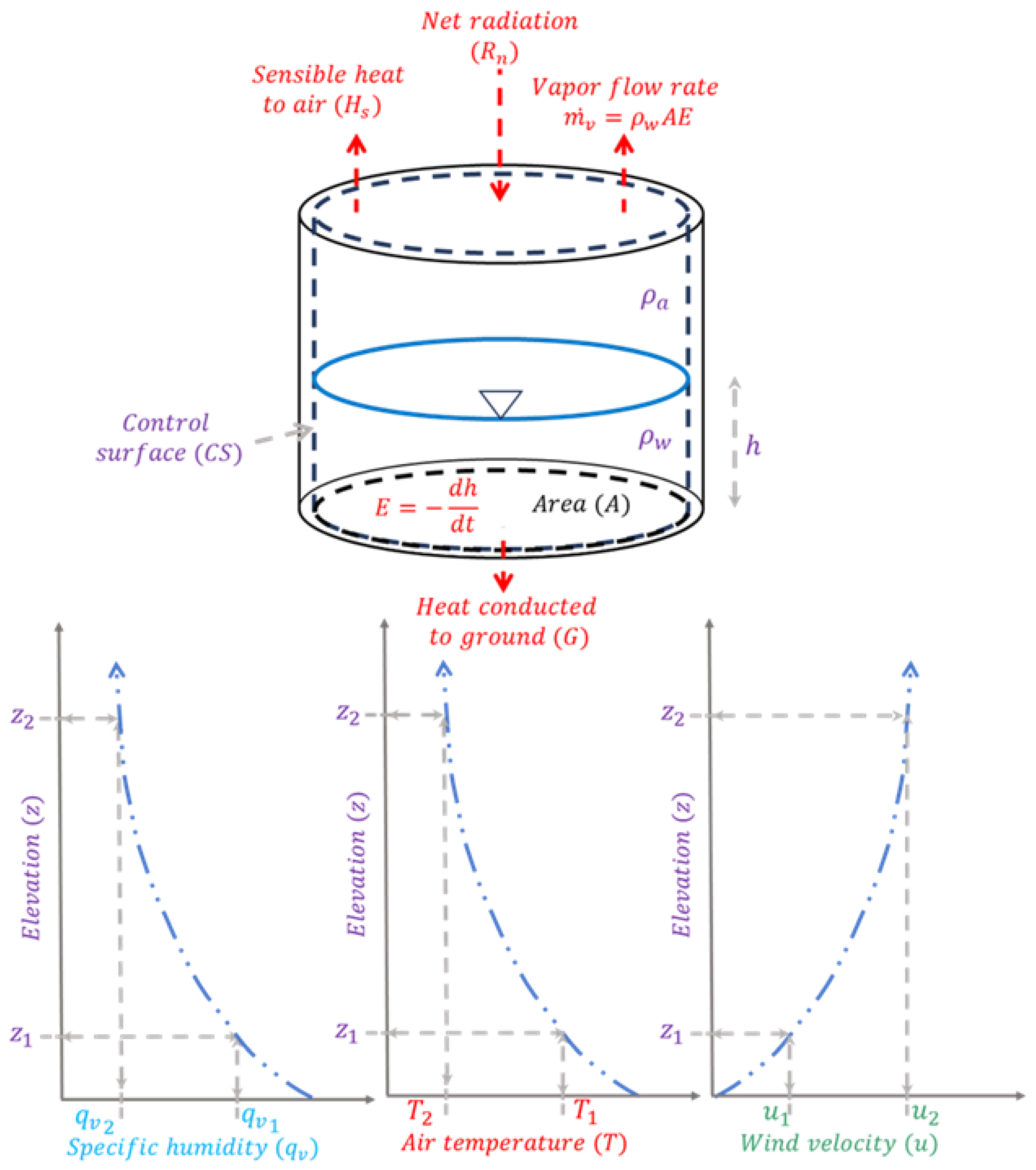
Now, the C V for any evaporation pan, as shown in Figure 5, contains water in both the liquid and vapor phases. For the liquid phase, the R T T can be applied; then B will be equal to the mass of liquid water, β = 1 , ρ = ρ w , and d B d t = m ˙ v , which is the mass flow rate of evaporation. In addition, for impermeable pan sides, the flow of liquid water across C S can be considered 0; i.e., the second term on the right side of the R T T will be 0. Therefore, for the liquid phase, the R T T can be written as
m ˙ v = ρ w A d h d t = ρ w A E
where E is the evaporation rate. Similarly, for the vapor phase, B will be equal to the mass of water vapor, β = q v , ρ = ρ a , and d B d t = m ˙ v . In addition, for a steady flow of air over the evaporation pan, the time derivative of water vapor stored within the C V is 0; i.e, first term on the right side of the R T T will be 0. Therefore, for the vapor phase, the R T T can be written with the help of Equation (17) as follows:
m ˙ v = ρ w A E = C S q v ρ a V d A
Therefore, E can be defined as the equivalent depth of water evaporated per unit time and can be expressed as
E = 1 ρ w A C S q v ρ a V d A
Similarly, Equation (4) can be applied to assess the energy balance of a hydrological system for water within the C V shown in Figure 5. In this context, the velocity is negligible, implying V = 0 ; the rate of work performed by the system ( d W d t ) is also negligible for the water in the evaporation pan, and its elevation (z) is minimal. Therefore, the R T T can be simplified to
d H d t = d d t C V e u ρ w d V = R n H s G
where R n represents the net radiation flux, H s denotes the sensible heat flux to the air, and G is the ground heat flux to the surface. Assuming the water temperature inside the C V remains temporally constant, the only change in the heat stored within the C V is the change in the internal energy of the water evaporated, which is equal to l v m ˙ v , where l v is the latent heat of vaporization. Hence, Equation (20) can be rewritten as R n H s G = l v m ˙ v , and Equation (17) can be used to help solve for E:
E = 1 l v ρ w ( R n H s G )
which is the energy balance equation for evaporation. If H s and G are both 0, then the evaporation rate E r can be calculated as E r = R n l v ρ w .
In addition to heat supply, the evaporation rate from an open water surface is influenced by the transport of vapor away from the surface. This transport rate depends on the humidity gradient near the surface and the wind speed across it [45,46,47,48,49,50,52,53,54,55]. The analysis of these processes can be carried out by integrating the equations that govern mass and momentum transport in the air. Consider, for this scenario, depicted by the C V in Figure 5, a horizontal plane with a unit area that is located at height z above the surface. Then, the mass vapor flux m ˙ v passing upward by convection through this plane can be defined by Equation (22) using the mass convection described earlier.
m ˙ v = ρ a K w d q v d z
where K w is the vapor eddy diffusivity. Similarly, the momentum flux upward through the plane can be defined by Equation (23) using the momentum convection described earlier.
τ = ρ a K m d u d z
Equations (22) and (23) can be combined, and substituting the differential forms for the z 1 -to- z 2 domain (see Figure 5) gives us
m ˙ v τ = K w ( q v 2 q v 1 ) K m ( u 2 u 1 )
Now using the logarithmic wind velocity profile (see Equation (11)), we can write
u * = τ ρ a = κ ( u 2 u 1 ) ln ( z 2 z 1 )
Substituting the value of τ into Equation (24) and rearranging gives
m ˙ v = K w κ 2 ρ a ( q v 1 q v 2 ) ( u 2 u 1 ) K m [ ln ( z 2 z 1 ) ] 2
which is commonly known as the Thornthwaite–Holzman equation for vapor transport [47,48,49,50,51,52,53,54,55]. If k w / K m = 1 and is constant, u 1 = 0 at the roughness height z 1 = z 0 , and the air is saturated with moisture there, and at height z 2 , the vapor pressure is e a , the ambient vapor pressure in the air, and the vapor pressure at the surface is taken to be e a s , the saturated vapor pressure corresponding to the ambient air temperature; then Equation (26) can be written as
m ˙ v = ρ w E a = 0.622 κ 2 ρ a ( e a s e a ) u 2 P [ ln ( z 2 z 0 ) ] 2
Therefore, the evaporation rate E a = B ( e a s e a ) , where B = 0.622 κ 2 ρ a u 2 P ρ w [ ln ( z 2 z 0 ) ] 2 . This vapor transfer coefficient B can vary from one place to another.
Evaporation can be computed using the aerodynamic method when the energy supply is not a limiting factor and using the energy balance method when vapor transport is not limiting [45,46,47,48,49,50,51,52,53,54,55]. However, since both factors typically impose limitations, a combination of the two methods is necessary. In the energy balance method, quantifying the sensible heat flux ( H s ) is challenging. Given that heat transfer occurs through convection in the air over the water surface, and water vapor is similarly convected, it is assumed that the vapor heat flux ( l v m ˙ v ) and the sensible heat flux ( H s ) are proportional. This proportionality constant is referred to as the Bowen ratio ( β = H s l v m ˙ v ). In addition, if G = 0 , Equation (21) can be written as R n = l v m ˙ v ( 1 + β ) . This Bowen ratio β can be calculated by coupling the convective transport equations for vapor mas and heat energy. Therefore, the heat energy flux can be defined by Equation (28) using energy convection, as described earlier.
H s = ρ a C p K h d T d z
where C p is the specific heat at constant pressure and K h is the heat diffusivity. Hence, Equations (22) and (28) can be combined, and substituting the differential forms for the z 1 -to- z 2 domain (see Figure 5) gives us
H s m ˙ v = C p K h ( T 2 T 1 ) K w ( q v 2 q v 1 )
Therefore, the Bowen ratio can be calculated as
β = C p K h p ( T 2 T 1 ) 0.622 l v K w ( e 2 e 1 ) = γ ( T 2 T 1 ) ( e 2 e 1 )
where γ is the psychrometric constant. If Δ is the gradient of the saturated vapor pressure curve at air temperature T a , then Equation (31) can be considered as the equation for the combined method of computing evaporation [46,47,48,49,50,52,53,54,55,56].
E = Δ Δ + γ E r + Δ Δ + γ E a
If the second term of Equation (31) is approximately 30 % of the first term, then Equation (31) is commonly known as the Priestley–Taylor evaporation equation, i.e., E = 1.3 Δ Δ + γ E r . Alternatively, the computation of the E T rate follows the same procedures as those used for open water evaporation, with modifications to consider the state of the vegetation and soil. Under specific climatic conditions, the fundamental rate is known as the reference crop E T , defined as the rate of E T from a broad area of green grass cover, 8 to 15 cm tall, uniformly high, actively growing, fully shading the ground, and well-watered. The potential E T for a different crop under the same conditions as the reference crop is determined by multiplying the reference crop E T E t r by a crop coefficient k c , which varies with the crop’s growth stage. The actual E T E t is obtained by multiplying the potential E T by a soil coefficient k s ( 0 k s 1 ): E t = k s k c E t r . The crop coefficient k c ranges from approximately 0.2 to 1.3 [1,46,47,48,49,50,52,54,55,56,57].
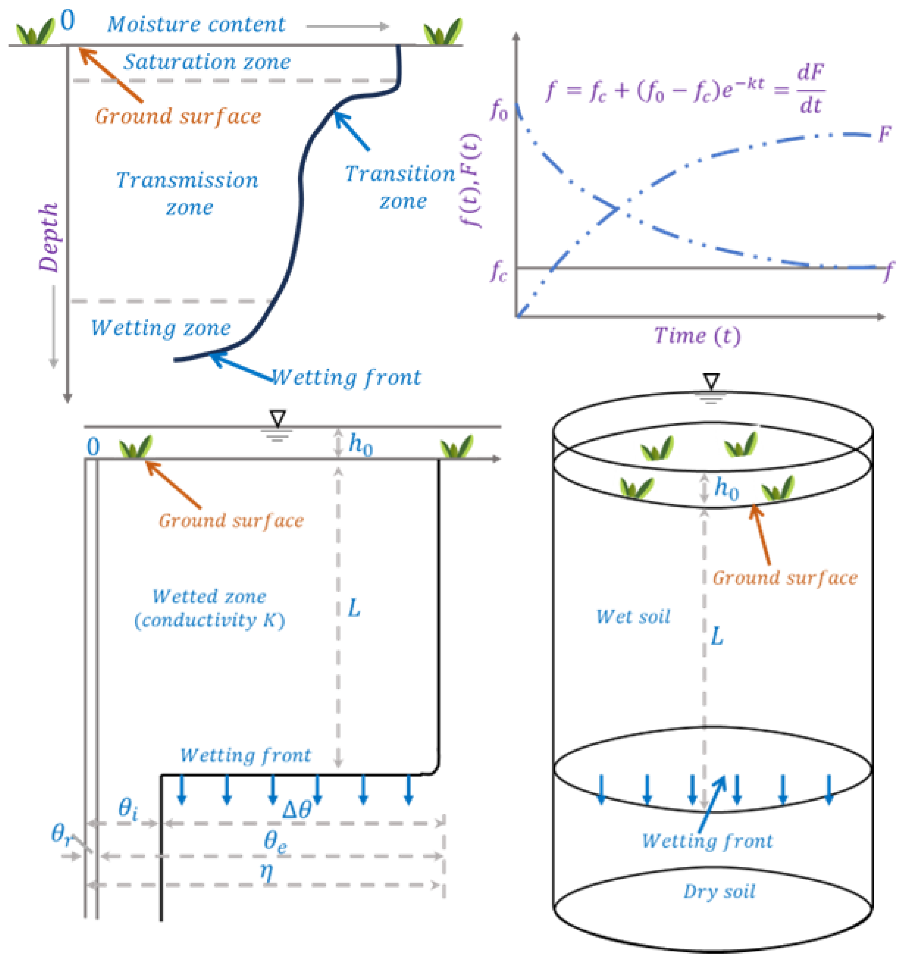
Three key processes are involved in the movement of water through soil: the infiltration of surface water into the soil as moisture, subsurface (unsaturated) flow through the soil, and groundwater (saturated) flow through soil or rock (see Figure 6). Soil and rock strata allowing water flow are termed porous media. Flow is unsaturated when the voids contain both air and water and saturated when voids are fully water-filled. The water table marks the surface where the water in a saturated porous medium is at atmospheric pressure. Below the water table, the pressure exceeds atmospheric pressure, while above it, capillary forces create a short capillary fringe of saturation, beyond which the medium is generally unsaturated, except after rainfall when temporary saturation from infiltration occurs. Subsurface and groundwater outflow happen when subsurface water reaches the surface, forming streams or springs. Soil moisture is depleted by E T as the soil dries [1,9,52,58,59,60,61,62,63,64,65,66,67,68,69,70,71,72,73,74,75,76].
Figure 6 illustrates a section in which solid particles occupy a portion of the cross-section, with the remaining part consisting of voids. Porosity, symbolized as η = volume of voids total volume , is generally in the ranges of 0.25 < η < 0.75 for soils, depending on the soil texture. Some voids are filled with water, while others contain air. The moisture content of the soil, denoted by θ = volume of water total volume , indicates the volume of water in the voids. Thus, 0 θ η ; when the soil is saturated, the soil moisture content equals the porosity. Furthermore, Figure 6 shows a C V with unsaturated soil, where the volume of water in the C V is θ d x d y d z . The Darcy flux, q = Q / A , measures the volumetric flow rate per unit area of soil. This discussion is limited to the vertical component of the Darcy flux (see Figure 6). Taking into account the R T T , the extensive property B represents the mass of soil water, leading to β = d B d m = 1 , and d B d t = 0 since no phase changes occur in the water. Therefore, the first and second terms of Equation (1) can be expressed as
d d t C V β ρ w d V = d d t ( ρ w θ d x d y d z ) = ρ w d x d y d z d θ d t
and
C S β ρ w V d A = ρ w q + q z d z d x d y ρ w q d x d y = ρ w d x d y d z q z
Hence, the R T T gives us the continuity equation for one-dimensional unsteady unsaturated flow in a porous medium:
θ t + q z = 0
This equation is relevant for flow at shallow depths beneath the land surface. At greater depths, such as in deep aquifers, variations in water density and porosity can occur due to changes in fluid pressure, and these must be considered when developing the continuity equation. In Equation (10), Darcy’s law is formulated to relate the Darcy flux q to the rate of head loss per unit length of a medium, S f , i.e., q = K S f . For vertical flow, if we denote the total head of the flow by h, then S f = h z , where the negative sign indicates that the total head decreases in the direction of flow due to friction. Thus, Darcy’s law is expressed as q = K h z . At this scale, Darcy’s law represents a steady uniform flow of constant velocity, where the net force on any fluid element is zero. For unconfined saturated flow, the only forces involved are gravity and friction. However, for unsaturated flow, the suction force binding the water to the soil particles through surface tension must also be included. When the void spaces are only partially filled with water, the water is attracted to the particle surfaces through surface adhesion. As more water is added to the porous medium, the air exits upwards, and the area of free surfaces within the medium diminishes until the medium is saturated, leaving no free surfaces within the voids and, consequently, no soil suction force. In an unsaturated porous medium, the part of the total energy possessed by the fluid due to soil suction forces is known as the suction head ψ [1,9,52,58,59,60,61,62,63,64,65,66,67,68,69,70,71,72,73,74,75,76]. Therefore, the total head is the sum of the suction and gravity heads, i.e., h = ψ + z , where the velocity is negligible. In this scenario, Darcy’s law can be expressed as
q = K ( ψ + z ) ) z = K d ψ d θ θ z + K = D θ z + K
where D is the soil water diffusivity. Equations (34) and (35) can be combined as follows:
θ t = z D θ z + K
which represents a one-dimensional version of the governing equation for transient unsaturated flow in a porous medium, often referred to as Richard’s equation [9,52,58,59,60,61,62,63,64,65,66,67,68,69,70,71,72,73,74,75,76,77]. In addition, infiltration in a watershed is influenced by spatial and temporal variations in soil moisture content. Infiltration is the process by which water enters the soil from the surface of the ground. Numerous factors affect the infiltration rate, including the surface soil condition and its land cover. Infiltration is a highly complex process that can only be approximated using mathematical equations. During the downward movement of water, there are four moisture zones: a saturated zone near the surface, a transmission zone of unsaturated flow with relatively uniform moisture content, a wetting zone where moisture decreases with depth, and a wetting front where the change in moisture content with depth is so significant that it appears as a sharp discontinuity between the wet soil above and the dry soil below. The infiltration rate f represents the speed at which water penetrates the soil surface, typically measured in inches per hour or centimeters per hour. When water pools on the surface, infiltration occurs at the potential infiltration rate. If the water supply rate (for example, rainfall) on the surface is below the potential infiltration rate, the actual infiltration rate will also be lower than the potential rate. Most infiltration models describe the potential rate. The cumulative infiltration F is the total depth of water that has infiltrated over a specified time period and can be represented as F = 0 t f ( τ ) d τ . Therefore, the infiltration rate is the time derivative of the cumulative infiltration, that is, f ( t ) = d F ( t ) d t .
One of the first infiltration models was proposed by Horton (1933, 1939), who noted that infiltration starts at an initial rate f 0 and decreases exponentially to a steady rate f c , expressed as f ( t ) = f c + ( f 0 f c ) exp k t , where k is a decay constant with dimensions [ T 1 ] [66,67]. Eagleson (1970) and Raudkivi (1979) demonstrated that Horton’s model can be derived from Richard’s Equation (36) by assuming that K and D are constants, unaffected by the soil moisture content [1,52]. Under these assumptions, Equation (36) simplifies to θ t = D 2 θ z 2 , which is a standard diffusion equation and can be solved to determine the moisture content θ as a function of time and depth. The Horton model is derived by solving for the moisture diffusion rate D θ z on the soil surface. Philip (1957, 1969) solved Richard’s equation under less restrictive conditions by allowing K and D to vary with the moisture content θ [71,72]. Philip used the Boltzmann transformation B ( θ ) = z t 1 / 2 to convert Equation (36) into an ordinary differential equation in B and solved it to obtain an infinite series for cumulative infiltration F ( t ) , approximated by F ( t ) = S t 1 / 2 + K t , where S is a parameter known as sorptivity, related to soil suction potential, and K is the hydraulic conductivity. Differentiating gives us f ( t ) = ( 1 / 2 ) S t 1 / 2 + K , and as t , f ( t ) K . The two terms in Philip’s equation represent the influences of the soil suction head and gravity head, respectively. For a horizontal soil column, soil suction is the sole force that draws water into the column, reducing Philip’s equation to F ( t ) = S t 1 / 2 .
Besides approximate solutions of Richard’s equation, Green and Ampt (1911) proposed a simplified approach (see Figure 7) in which a more approximate physical theory has an exact analytical solution [9]. In this theory, it is assumed that the wetting front is a sharp boundary that divides the soil with a moisture content θ i below from the saturated soil with a moisture content η above. The wetting front has penetrated to a depth L in time t since the infiltration began. The water is ponded to a small depth h 0 on the surface of the soil (see Figure 7). If the soil initially had a moisture content θ i throughout its entire depth, the moisture content will increase from θ i to η as the wetting front passes [1]. Therefore, the increase in water stored within the C V as a result of infiltration is L ( η θ i ) for a unit cross-section; by definition, this quantity is equal to F. Hence, F = L ( η θ i ) = L Δ θ . Also, Darcy’s law may be expressed as q = K h z = K h 1 h 2 z 1 z 2 , where points 1 and 2 are located, respectively, at the ground surface and just on the dry side of the wetting front, and q is constant throughout the depth and q = f , and h 1 = h 0 and h 2 = ψ L due to the dry soil below the wetting front. Hence, Darcy’s law may be expressed as
f = K h 0 ( ψ L ) ) L
Now, if h 0 is negligible compared to ψ and L or if ponded water becomes surface runoff (usual assumption for watershed hydrology), then Equation (37) gives
f K ψ + L L = K ψ Δ θ + F F f = d F d t = K 1 + ψ Δ θ F
Equation (38) can be expressed as a differential equation as follows:
F F + ψ Δ θ d F = K d t
Now, splitting the left-hand side into two parts and integrating gives
0 F ( t ) 1 ψ Δ θ F + ψ Δ θ d F = 0 t K d t F ( t ) ψ Δ θ ln 1 + F ( t ) ψ Δ θ = K t
The Green–Ampt equation for cumulative infiltration can be solved using either the method of successive substitution or the Newton–Raphson method. To apply this model, estimates of hydraulic conductivity K, porosity η , and wetting front soil suction head ψ are needed. These can be expressed as a logarithmic function of effective saturation S e , where S e = available moisture content maximum possible moisture content = θ θ r η θ r . Here, η θ r is known as the effective porosity θ e and Δ θ = ( 1 S e ) θ e .
These methods assume that water is ponded to a shallow depth on the soil surface, making all the water available for infiltration. However, during rainfall, water will only pond on the surface if the intensity of rainfall exceeds the soil’s infiltration capacity. The ponding time t p is the time elapsed from the start of rainfall to when water begins to pond on the soil surface. Before ponding time ( t < t p ), the rainfall intensity is less than the potential infiltration rate, and the soil surface remains unsaturated. Ponding starts when the rainfall intensity surpasses the potential infiltration rate. At this moment ( t = t p ), the soil surface becomes saturated. As rainfall continues ( t > t p ), the saturated zone extends deeper into the soil, and overland flow occurs from the ponded water. As illustrated in Figure 8, the cumulative infiltration at the ponding time t p is given by F p = i t p , and the infiltration rate by f = i .

5. Hydrologic Analysis

This section reviews surface water flow, the rainfall–runoff process, hydrograph analysis, and unit hydrograph theory. During a storm, precipitation contributes to various storage and flow processes. Initially, a significant portion is retained in surface and soil moisture storage. Storage can be classified as retention (long-term, lost via evaporation) or detention (short-term, depleted by flow). As detention storage fills, flow occurs via unsaturated flow in the vadose zone, groundwater flow in saturated aquifers, and overland flow. Channel flow integrates these contributions, making streamflow measurement a key task in hydrology.
Precipitation reaching streams does so via overland and subsurface flow. Horton [66] defined overland flow as precipitation exceeding the soil’s infiltration capacity f, with excess rainfall producing runoff at a rate of ( i f ). Hortonian overland flow occurs on impervious surfaces or areas with low infiltration, whereas saturation overland flow results from subsurface saturation near stream banks and hillslope bases. Due to low subsurface flow velocity, not all watershed areas contribute to streamflow during a storm.
A streamflow hydrograph represents discharge over time, integrating watershed physiographic and climatic factors. The annual hydrograph depicts long-term precipitation–evaporation–streamflow balance, while event-based hydrographs reveal direct runoff and baseflow recession patterns. Excess rainfall, or effective rainfall, excludes retained or infiltrated precipitation, generating direct runoff under Hortonian assumptions. The excess rainfall hyetograph ( E R H ), derived by subtracting losses (e.g., infiltration, interception) from total rainfall, is central to rainfall–runoff analysis. When streamflow data are available, excess rainfall can be estimated via the ϕ - i n d e x , a constant abstraction rate yielding an E R H depth equal to the direct runoff depth r d . In this case, the ϕ - i n d e x provides a simpler alternative to complex infiltration equations. It represents a constant rate of abstraction that results in an E R H with a total depth equal to the r d over the watershed. The value of ϕ is determined by selecting a time interval of length Δ t , identifying the number of intervals (M) in which rainfall contributes to direct runoff, subtracting ϕ Δ t from the observed rainfall in each interval, and adjusting the values of ϕ and M as needed to ensure that the total depths of direct runoff and excess rainfall are equal.
r d = m = 1 M ( R m ϕ Δ t )
where R m is the observed rainfall (in) in time interval m. These abstractions can also be taken into account using runoff coefficients. The most widely accepted definition of a runoff coefficient is the ratio of the maximum direct runoff rate to the average intensity of rainfall during a storm. Alternatively, a runoff coefficient can be described as the ratio of runoff to rainfall over a specified period of time. Runoff coefficients are typically applied to storm rainfall and runoff but can also be used for monthly or yearly rainfall and streamflow data. If m = 1 M R m represents the total rainfall and r d represents the corresponding depth of runoff, then the runoff coefficient is defined as C = r d m = 1 M R m . Abstractions in hydrology include precipitation interception by vegetation, surface depression storage, and soil infiltration. The extent of interception and depression storage depends on vegetation and ground surface characteristics. Abstraction rates from rainfall are typically derived from streamflow hydrographs; if unavailable, they are estimated by calculating infiltration and separately accounting for interception and depression storage. The Soil Conservation Service (SCS) of the USDA (now the Natural Resources Conservation Service, NRCS) developed a method to compute abstractions from storm rainfall. For an entire storm, the depth of excess precipitation or direct runoff P e P ; similarly, once runoff begins, the additional depth of water retained in the watershed F a is less than or equal to some potential maximum retention S. An initial amount of rainfall I a (initial abstraction before ponding) exists for which no runoff will occur, making the potential runoff P I a . The hypothesis for this method is that the ratios of the two actual quantities are equal to the two potential quantities, which means that F a S = P e P I a , and according to the continuity principle, P = P e + I a + F a . Additionally, through the analysis of numerous small experimental watersheds, the relation I a = 0.2 S was established. Consequently, the fundamental equation for calculating the depth of excess rainfall or direct runoff from a storm using this method is given by
P e = ( P I a ) 2 P I a + S = ( P 0.2 S ) 2 P + 0.8 S
By plotting the values of P and P e across various watersheds, the S C S ( N R C S ) identified a specific kind of curve. To standardize these curves, a dimensionless curve number C N was introduced, with a range of 0 C N 100 . For impervious and water surfaces, C N = 100 , while for natural surfaces, C N 100 . The relationship between the curve number ( C N ) and S is given by
S = 1000 C N 10
This C N value is determined based on the hydrologic soil group (A, B, C, or D), land use, treatment, and hydrological condition of the area in question. Hydrologic soil groups are categorized by their infiltration rates, with Group A soils having high infiltration rates and Group D soils having very low rates. Land use and treatment refer to the type of vegetation or urban development present, while the hydrological condition refers to the soil moisture content prior to the rainfall event.
The movement of water across a watershed surface is a complex phenomenon that changes in all three spatial dimensions and over time. Two primary flow types can be identified: overland flow and channel flow. Overland flow is characterized by a thin sheet of water moving over a broad surface, whereas channel flow involves a more narrow stream of water flowing in a confined path, often referred to as open-channel flow (refer to [2]). In a natural watershed, overland flow is the initial mechanism of surface flow, governed by the principles of continuity and momentum. This thin sheet flow occurs at the upper ends of slopes before concentrating into recognizable channels. Consider a flow over a uniform plane where rain is falling with an intensity i and infiltration is occurring at a rate f. Enough time has elapsed since the beginning of rainfall, such that all flows have become steady. The plane, which has a unit width and length L o , is inclined at an angle θ to the horizontal, with a slope given by S 0 = tan θ . The rainfall contributes an inflow to the C V given by i L o cos θ , while the outflow comprises f L o cos θ due to infiltration and V y resulting from overland flow. The depth y is quantified perpendicularly to the bed, and the velocity V is along the bed’s parallel. Therefore, the continuity equation is expressed as
f L o cos θ + V y i L o cos θ = 0 q 0 = V y = ( i f ) L o cos θ
where q 0 represents the discharge per unit width. Conversely, using the conservation of momentum, the average velocity V can be expressed as V = g S o y 2 3 ν , where ν signifies the kinematic viscosity of water and S o = S f = h f L , corresponding to the Darcy–Weisbach equation for flow resistance with the friction factor f = 96 R e , wherein the Reynolds number R e = 4 V R ν and R = y . In the case of laminar sheet flow under rainfall, the friction factor escalates with the precipitation rate. It can be hypothesized that f has the structure C L R e , with C L being a resistance coefficient influenced by i as C L = 96 + 108 i 0.4 . Consequently, using Equation (44), the sheet flow depth on a uniform surface can be expressed as
y = f q o 2 8 g S o 1 / 3
Equation (45) can be reformulated in a broader way as y = α q o m . For laminar flow, m = 2 / 3 , and α = f 8 g S o 1 / 3 . According to Emmett’s research, the Darcy–Weisbach friction factor f varies from 20 to 200 for overland flow observed at field sites. When the flow becomes turbulent, the friction factor becomes independent of the Reynolds number and dependent only on the roughness of the surface (Manning’s n). Therefore, for turbulent flow, m = 3 / 5 , and α = n 1.49 S o 1 / 2 3 / 5 or in, SI units, α = n 0.6 S o 0.3 . The travel time of flow from one point on a watershed to another can be deduced from the flow distance and velocity [1].
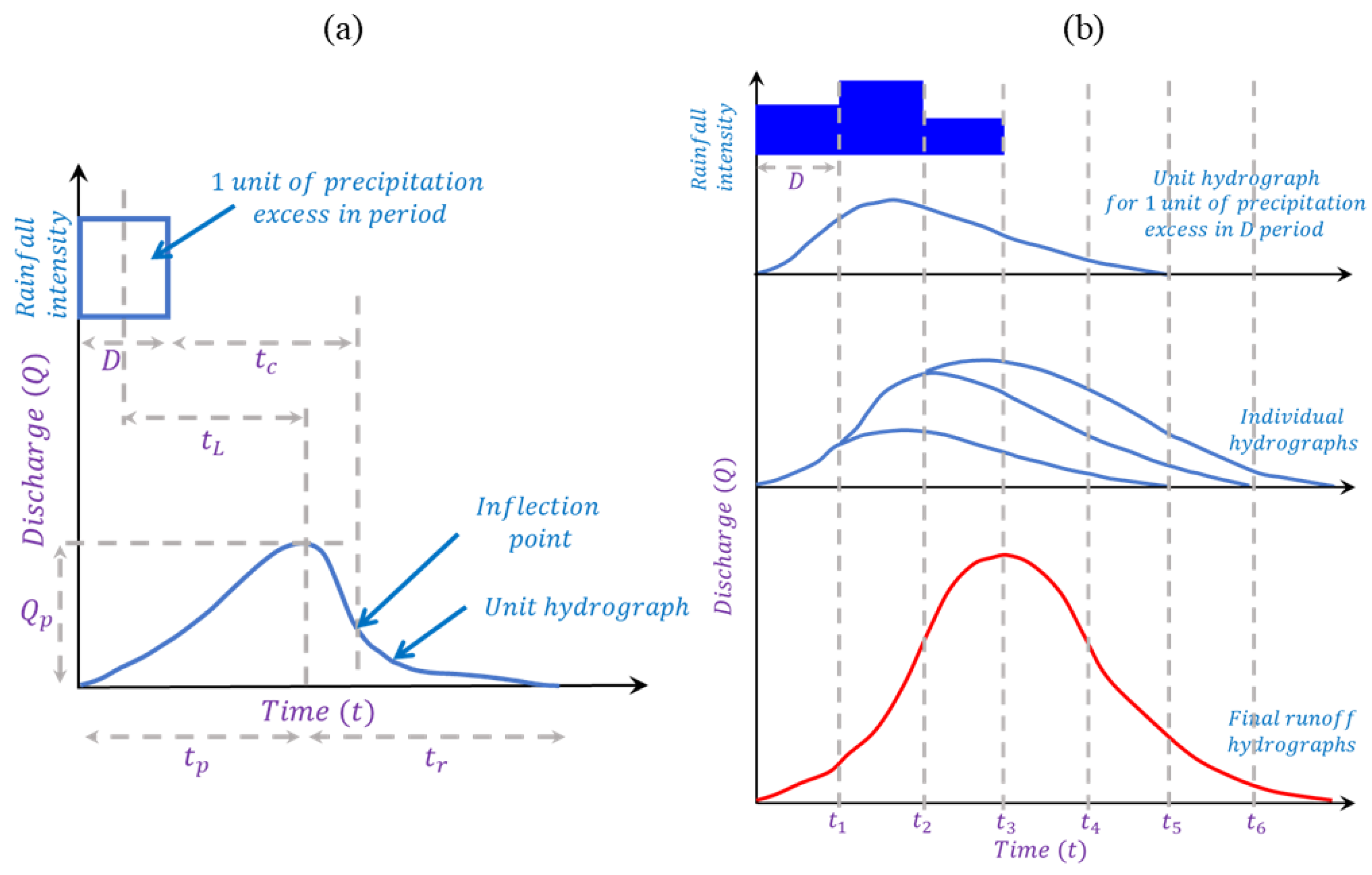
In watershed hydrology, the concept of an impulse response function ( I R F ) is closely related to the unit hydrograph ( U H ), both of which are essential for understanding how a watershed responds to a unit input of precipitation. A unit hydrograph is the direct runoff hydrograph resulting from one unit (usually 1 inch or 1 cm) of excess rainfall uniformly distributed over the watershed for a specified duration (typically one hour). It represents the time distribution of runoff at the outlet of a watershed due to a unit input of rainfall (see Figure 9). This makes it a powerful tool for predicting streamflow from different rainfall events. The unit hydrograph is the unit pulse response function of a linear hydrologic system. In the context of watershed hydrology, the I R F can be seen as a mathematical representation of U H . The I R F describes the output (runoff) response of the system (watershed) to a single instantaneous unit input of rainfall (impulse). The I R F , denoted as h ( t ) , is the hydrograph generated by a Dirac delta function (a spike in rainfall) applied to the watershed. If the rainfall input r ( t ) is represented as a time series, the resulting runoff q ( t ) can be obtained by convolving the input with the I R F :
q ( t ) = 0 h ( τ ) r ( t τ ) d τ
This convolution equation illustrates how the runoff at any time t is a result of the entire past rainfall history weighted by the I R F . If the rainfall input is divided into discrete pulses r [ n ] at time intervals Δ t , the runoff q [ n ] at time step n can be represented by the convolution of the discrete pulse response function h [ n ] with the rainfall input:
q [ n ] = k = 0 n h [ k ] . r [ n k ]
Here, h [ n ] can be seen as the discrete pulse response function ( D P R F ), which describes how much of the input pulse at time n k contributes to the runoff at time n. When observed rainfall and runoff data are insufficient to derive a unit hydrograph, synthetic unit hydrographs are utilized (see Figure 9). These hydrographs are created using empirical correlations that connect features of the watershed (such as area, slope, and shape) to the hydrograph form. Two widely used types are the Snyder unit hydrograph and the S C S unit hydrograph. The Snyder unit hydrograph is an empirical method introduced by F.F. Snyder [78]. The unit hydrograph is derived using the properties of the basin, focusing on the lag time ( t L ), which is the duration between the centroid of effective rainfall and the peak of the unit hydrograph. The peak discharge Q p and the time to peak t p can be calculated with the formulas Q p = C p A t p and t p = C t t L , where C p and C t are coefficients dependent on watershed properties, and A is the watershed’s area. Alternatively, the S C S unit hydrograph, developed by the Soil Conservation Service (now NRCS—Natural Resources Conservation Service) in the 1950s, is based on a dimensionless hydrograph. The S C S approach assumes a standard dimensionless unit hydrograph where time to peak is a function of the lag time t L , and peak discharge is linked to the watershed area. The related equations are Q p = 484 A t p , with t p = 0.6 t L , and Q p measured in cubic feet per second per inch of rainfall. The S C S ’s lag methodology is detailed as follows:
t L = L 0.8 ( S + 1 ) 0.7 1900 Y 0.5 t c = 5 3 t L t c = L 0.8 ( S + 1 ) 0.7 1140 Y 0.5 t c = L 3600 v
in which t c represents the time of concentration (h), S denotes the potential maximum retention ( i n ), Y indicates the slope of the watershed (%), L is the distance of the stream from the outlet to the upstream limits of the basin ( m i ), and v represents the velocity (ft/s). The dimensionless nature of the S C S hydrograph allows it to be scaled to different time frames and amounts of rainfall, providing practical versatility. It usually takes on a triangular or trapezoidal form, making calculations simpler while maintaining a reasonable degree of accuracy for various hydrologic applications. In addition, hydrographs can also be generated directly from the R N as previously described. Recently, researchers have designed a method to accurately produce hydrographs for a rainfall event using a complex network framework (refer to [15]). Other parameters useful for hydrologic analysis are the drainage density ( D d ) and the length of overland flow. D d is the ratio of the total length of the stream channels in a watershed to its area (A).

6. Statistics of Watershed Hydrology

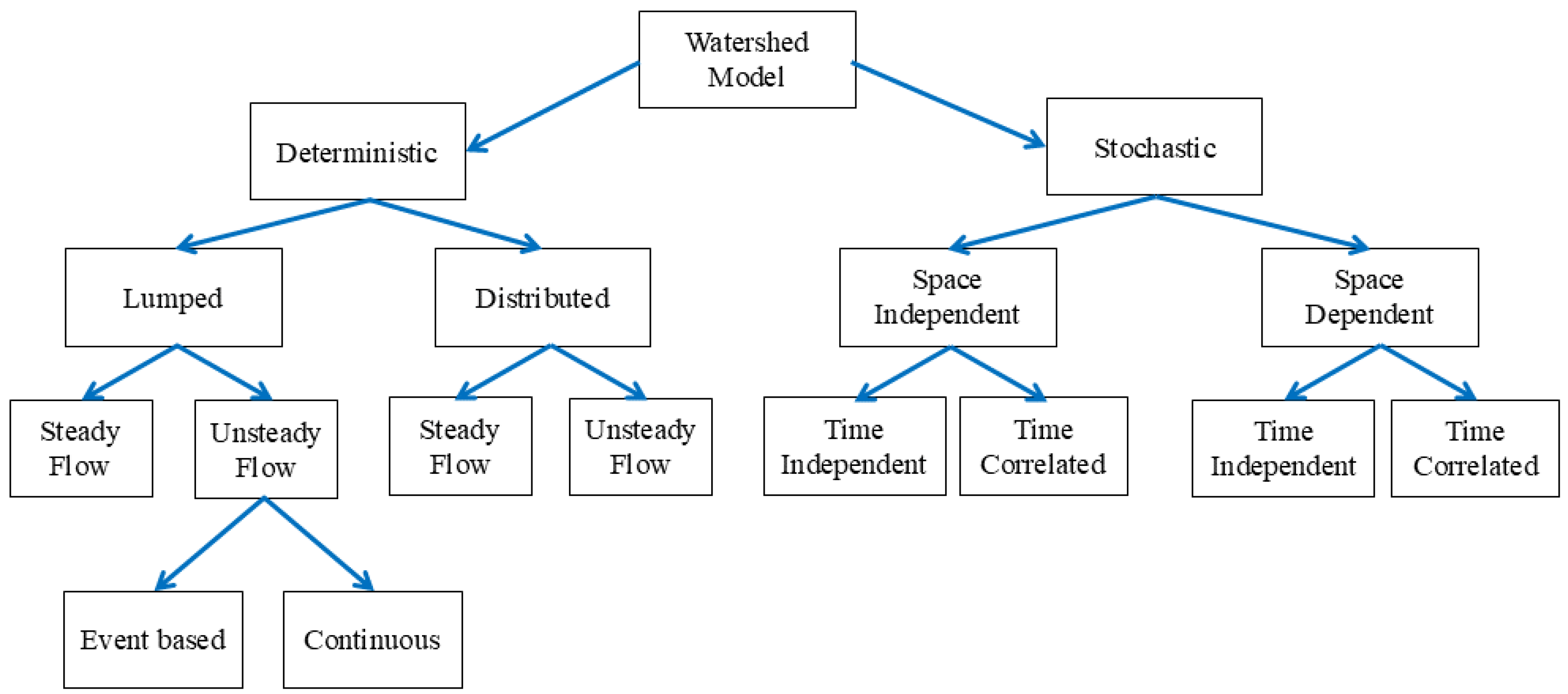
Statistics are integral to watershed hydrology and offer essential tools to analyze, model, and forecast hydrological phenomena. Deterministic models in watershed hydrology predict variables such as water levels and flow by utilizing fixed inputs and equations, thereby producing a single outcome based on specific initial conditions without considering natural uncertainties. In contrast, probabilistic or stochastic models incorporate elements of randomness and uncertainty, applying statistical methods to capture variability in inputs and processes. This probabilistic approach generates a range of possible outcomes, each with an associated probability, thereby more accurately mirroring the inherent variability and unpredictability of hydrological systems. Random variables ( R V s) are essential for probabilistic or stochastic models. Descriptive statistics encapsulate key characteristics of R V s, including central tendency and dispersion, and are instrumental in the frequency analysis of precipitation and streamflow data. Probability distributions, such as normal, log-normal, Gumbel, and gamma distributions, encapsulate the variability and uncertainty inherent in hydrological data. Inferential statistics, which encompasses hypothesis testing and regression analysis, facilitate predictions about populations based on sample data. Time-series analysis, which includes trend analysis, seasonal decomposition, and autoregressive models, aids in comprehending and forecasting temporal patterns in hydrological data. Extreme value analysis, crucial for assessing rare events like floods and droughts, involves estimating return periods and analyzing peak-over-threshold data. Hydrologic frequency analysis estimates the probability and frequency of events, such as floods, using distributions like Log-Pearson Type III. Spatial statistics, including geostatistics and spatial correlation, are employed to examine spatial patterns, while multivariate statistics, such as principal component analysis and cluster analysis, manage multiple variables concurrently to elucidate complex hydrological phenomena. Stochastic hydrology employs probabilistic methods, such as Monte Carlo simulations, to model hydrologic processes under uncertainty. Model calibration and validation engage statistical methods to ensure model accuracy and predictive capability, utilizing goodness-of-fit tests and cross-validation.
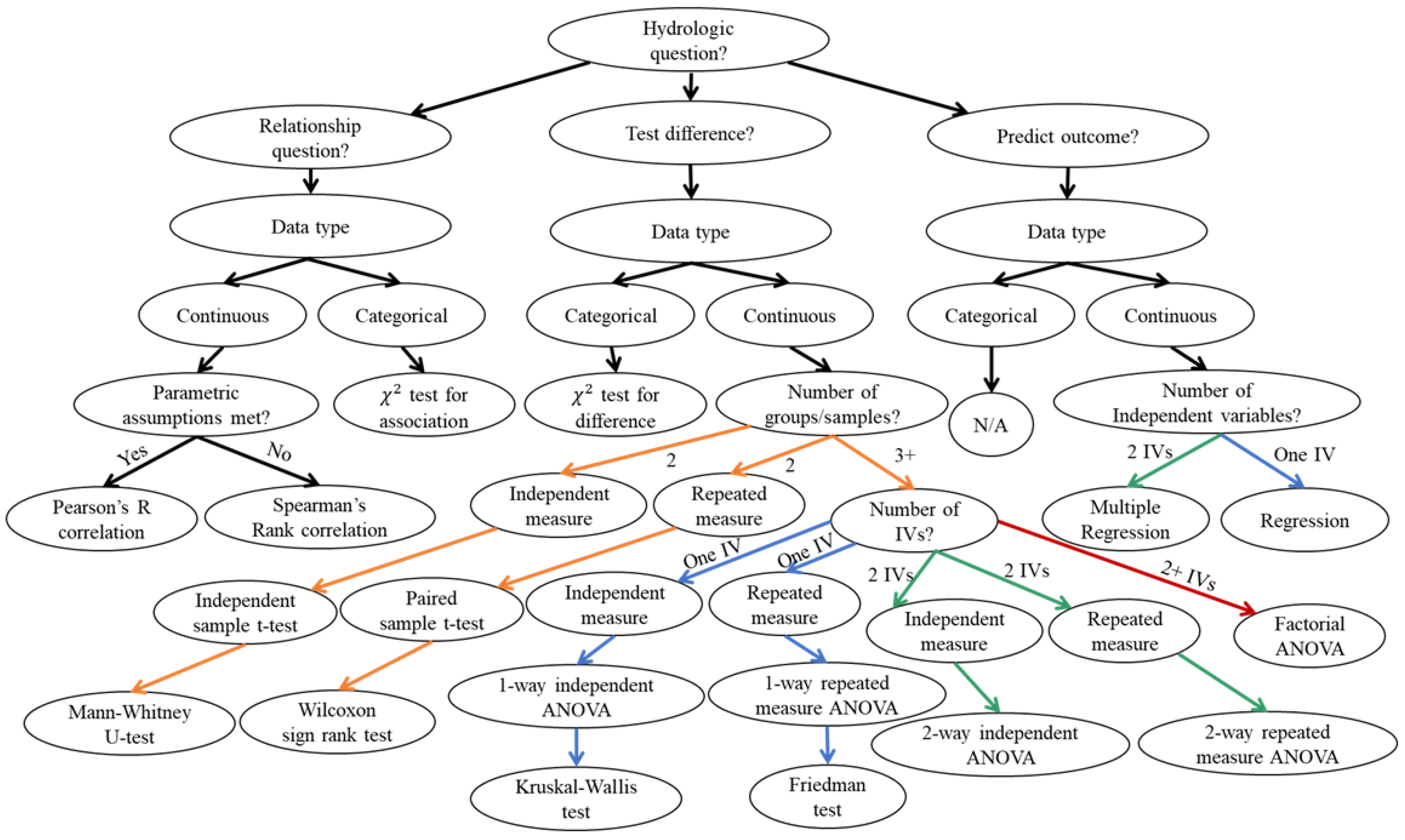
A range of statistical tests are used to analyze data related to water resource questions, including precipitation, streamflow, and groundwater levels. Parametric tests, such as the t-test, ANOVA, and regression analysis, compare group means and elucidate relationships among variables (see Figure 10). Nonparametric tests, such as the Mann–Whitney U test, the Kruskal–Wallis test, and Spearman rank correlation, are applied when the data do not conform to a normal distribution. Goodness-of-fit tests, including the Chi-Square and Kolmogorov–Smirnov tests, determine how well the data fit a theoretical distribution. Time-series analysis encompasses the autocorrelation function, seasonal decomposition, and ARIMA modeling for forecasting and trend analysis. The Mann–Kendall trend test and Sen’s slope estimator are specifically utilized for identifying and estimating trends in hydrologic time-series data. Extreme value analysis, utilizing Gumbel and Generalized Extreme Value ( G E V ) distributions, is essential for modeling extreme events such as floods. Hypothesis testing methods, including the Z test and the Shapiro–Wilk test, assess population means and data normality. In the domain of watershed hydrology, these statistical methods are applied to studies of water balance, runoff modeling, sediment transport estimation, nutrient loading assessments, and climate change impact evaluations, enabling hydrologists to make informed decisions based on comprehensive data analysis and modeling.
The frequency analysis of hydrological data encompasses statistical methodologies to model and forecast the probabilities and recurrence intervals of extreme phenomena such as floods, droughts, precipitation, and streamflow. This analytical process initiates with the collection and preparation of data to maintain quality and consistency, followed by the selection of an appropriate probability distribution, such as normal, log-normal, Gumbel, or Generalized Extreme Value ( G E V ). Table 1 delineates the probability density functions and variable ranges for commonly employed distributions and provides equations for estimating distribution parameters from sample moments. Subsequently, the parameters of the chosen distribution are estimated using techniques such as the method of moments, maximum likelihood estimation, or L-moments. Goodness-of-fit tests, including the χ 2 , K o l m o g o r o v S m i r n o v , and A n d e r s o n D a r l i n g tests, are utilized to assess the conformity of the distribution to the data. The analysis advances by computing the probability of exceedance and return periods for varying event magnitudes, depicted through frequency curves, probability plots, and log-probability plots. This methodology aids in evaluating risk and reliability by computing the likelihood and dependability of extreme events over specified temporal periods. Here, risk (R) is defined as the probability of at least one occurrence of an event of a specified magnitude within a given period (n years), articulated as R = 1 ( 1 P ) n , while reliability ( R e l ) is defined as the probability that an event of a specified magnitude will not occur within the given period, articulated as R e l = 1 R . Applications of frequency analysis in hydrology encompass flood frequency analysis for the design of flood control structures, drought frequency analysis for water resource management, precipitation frequency analysis for urban drainage systems, and low-flow frequency analysis for ecological assessments and wastewater discharge permits. This comprehensive approach fosters informed decision-making in water resource management and infrastructure design, thereby enhancing preparedness for extreme hydrological events.

7. Flow Routing on Watershed

The objective of this section is to review the concepts and methods of lumped and distributed flood routing, along with providing insight into the Muskingum method and the physical phenomena behind the Saint-Venant equations ( S V E s).
Flow routing in hydrology refers to the process of determining the time and quantity of flow at various points in a river system. This process is essential for flood forecasting, water resource management, and environmental protection. There are two primary types of flow routing: lumped and distributed. Lumped flow routing is a fundamental concept in hydrological modeling, used to predict how water moves through a watershed or a river system. Unlike distributed models, which consider spatial variability in parameters, lumped flow routing treats the entire watershed as a single unit. This simplification is particularly useful for large-scale hydrological predictions where detailed spatial data may not be available. Lumped flow routing is governed by the principle of mass conservation, also known as the continuity equation. The fundamental idea is that the inflow into a system, minus the outflow, should equal the change in storage within the system. This can be mathematically expressed as
d S ( t ) d t = I ( t ) Q ( t )
where S ( t ) is the storage in the system at time t, I ( t ) is the inflow rate at time t, and Q ( t ) is the outflow rate at time t. This equation forms the basis of lumped flow routing, encapsulating the essence of how water is stored and released in a watershed. The Linear Reservoir Model is one of the simplest lumped flow routing models. It assumes a direct proportionality between the storage S ( t ) and the outflow Q ( t ) . The model is expressed as Q ( t ) = 1 K S ( t ) , where K is a constant representing the storage coefficient. Substituting this into Equation (49), we can write
d S ( t ) d t = I ( t ) 1 K S ( t )
This differential equation can be solved to find S ( t ) and subsequently Q ( t ) , given an inflow I ( t ) . The Muskingum method is another widely used lumped flow routing model. It incorporates both storage and the concept of a linear relationship between inflow and outflow. The storage S ( t ) is expressed as S ( t ) = K [ X I ( t ) + ( 1 X ) Q ( t ) ] , where X is a weighting factor ( 0 X 0.5 ) that represents the distribution of storage between inflow and outflow. Combining this with Equation (49), we can write
I ( t ) Q ( t ) = K [ X I ( t ) + ( 1 X ) Q ( t ) ] Δ t
This equation can be solved iteratively to find Q ( t ) , given I ( t ) . Lumped flow routing models are extensively used in hydrological studies, particularly for flood forecasting. Their simplicity allows for rapid computation and easy calibration, making them ideal for real-time applications. For example, the Linear Reservoir Model is often used in watersheds with a single dominant storage feature, such as a large lake or reservoir. The Muskingum method, on the other hand, is favored in river systems with more complex flow dynamics. While lumped flow routing models are powerful tools, they have limitations. The assumption of spatial homogeneity may not hold in all watersheds, particularly those with significant variations in topography, land use, and soil types. Furthermore, the choice of parameters such as K and X requires careful calibration against the observed data to ensure accuracy [1,79]. In contrast, distributed routing takes into account the spatial variations in flow within the channel or watershed. It includes variations in channel characteristics, slope, and other hydraulic factors that affect the flow at various locations. The mathematical formulation of distributed flow routing is based on the principles of mass and momentum conservation, often expressed through the Saint-Venant equations ( S V E s). These equations are a set of partial differential equations that describe unsteady, one-dimensional flow in open channels. The continuity equation, which represents the conservation of mass, is given by
A t + Q x = q L
where A ( x , t ) is the cross-sectional area of flow at a distance x along the channel and time t, Q ( x , t ) is the discharge or flow rate, q L ( x , t ) is the lateral inflow per unit length of the channel, A t represents the change in flow area over time, and Q x represents the change in discharge along the length of the channel. In addition, the momentum equation, which represents the conservation of momentum, is given by
Q t + x Q 2 A + g A h x + g A S f = 0
where h ( x , t ) is the flow depth, Q t represents the change in discharge over time, x Q 2 A represents the change in momentum flux along the channel, g A h x represents the gravitational force acting on the flow, and g A S f represents the frictional resistance (see details in [41]). The S V E s are nonlinear partial differential equations that are difficult to solve analytically, except for highly simplified cases. Therefore, numerical methods are typically employed to solve these equations. Some common numerical methods include the finite difference method ( F D M ) to approximate the derivatives in S V E s using finite differences. The channel is discretized into a grid, and the equations are solved iteratively at each grid point (see [2,80]). The finite volume method ( F V M ) divides the channel into control volumes, and the fluxes of mass and momentum are calculated across the boundaries of these volumes. This method is particularly useful for problems with complex geometries and discontinuities in the flow. The method of characteristics transforms the S V E s into a set of ordinary differential equations along characteristic lines. This method is powerful for solving hyperbolic systems of equations, such as S V E s, but it can be complex to implement.
Kinematic wave theory simplifies the full S V E s by neglecting the inertial terms, focusing on the relationship between flow discharge Q and flow area A or depth h. The theory is particularly useful for analyzing shallow water waves where inertial effects are minimal, such as flood routing or overland flow. The basic form of the kinematic wave equation is h t + c h x = 0 , where c is the wave celerity, defined as Q A . In the context of flood routing, the kinematic wave equation can be used to model the propagation of flood waves through river channels. The flow discharge Q can be expressed as a function of flow depth h using a power law Q = α h m . Substituting this into the kinematic wave equation gives
h t + α m h m 1 h x = 0
This equation provides a framework for predicting the movement of a flood wave along a river channel, considering the relationship between depth and discharge. Diffusive wave routing adds a level of complexity by incorporating the effects of flow diffusion. This method still neglects the inertial terms but considers the pressure gradient term in the momentum equation. The continuity equation remains the same, but the diffusive wave momentum equation, which incorporates pressure forces, is given by h x = S f S o S f . For practical purposes, the S V E s are often linearized and simplified as
h t + c h x = D c 2 h x 2
where D is the diffusion coefficient. The inclusion of the diffusion term leads to a spread or attenuation of the wave as it travels downstream. The wave speed is still primarily determined by the kinematic wave speed c, but the shape of the wavefront is influenced by the diffusion coefficient. Diffusive wave routing is suitable for channels where flow attenuation is significant, such as on mild to moderate slopes, or where the flow depth changes gradually. Dynamic wave routing is a more comprehensive method compared to kinematic wave theory, as it includes inertial and pressure forces. The governing equations are the full S V E s. Because the full dynamic wave equations are nonlinear and coupled, numerical methods are typically employed to discretize the equations and solve them iteratively.
Smoothed Particle Hydrodynamics ( S P H ) is another widely used mesh-free Lagrangian method in hydrology for simulating free-surface and multi-phase flows. It is particularly advantageous for modeling complex hydrodynamic phenomena, such as dam breaks, flood propagation, and sediment transport, where traditional grid-based methods struggle with deformable boundaries and high-gradient regions (see [81]). The S P H approach discretizes the fluid domain into particles, which carry physical properties and interact based on kernel functions, enabling an accurate representation of flow dynamics in natural water bodies (see [82]). Due to its adaptability to irregular geometries and capability to handle large deformations, S P H has gained significant attention and application in hydraulic and hydrological modeling [83,84].

8. Watershed Models

A model is a simplified representation of reality, constructed using hypotheses and mathematical equations. The models are derived from both experimental data and theoretical frameworks that are integrated through computational methods. There are two primary types of models: conceptual and mathematical. The conceptual models describe hydrologic processes, usually by using qualitative tools, often based on graphs, that represent key elements of a system, including its components, processes, linkages, and interactions. Conceptual models can serve as an initial step for hypothesis testing and the development of mathematical models. Additionally, they can act as a framework for future monitoring, research, and management actions at a specific site. In contrast, mathematical models define modeling as the use of mathematics to explain and predict natural phenomena and processes. Mathematical modeling can include words, diagrams, mathematical notation, and physical structures. The goal is to improve scientific understanding through the application of mathematical models using high-performance computers. Mathematical modeling of watersheds is crucial for addressing various environmental and water resource challenges. The effective planning, designing, and managing of water resource systems depend on accurate water resource assessment and impact prediction, which necessitates modeling. Developing such models is a complex task that requires a thorough understanding of the system being modeled, the user’s objectives and goals, and the information needed, as well as a blend of analytical and programming skills (UNESCO, 2005). Developing a working model for a real-world problem involves a systematic process and steps. This process begins with simplifying the real-world problem into a mathematical model that represents the problem and the physical processes of the system using mathematical equations. The mathematical model is then converted into a computational model to simulate the different hydrologic processes of a watershed. The conclusions and results from these simulations are interpreted and compared with the observations to refine the working model, which informs further simplification and representation, perpetuating the cycle. Various statistical metrics are commonly used to quantify a model’s performance. For example, the mean is the average or expected value, while variance measures the average squared deviations from the mean and can be used as means of statistically evaluating the performance of the model. Reliability is the probability of a system remaining satisfactory, and resilience is the probability of returning to a satisfactory state after an unsatisfactory one. Robustness refers to a system’s adaptability beyond its design conditions, and Vulnerability indicates the expected extent of failure during an unsatisfactory state. Consistency relates to the reliability or uniformity of successive results. The watershed concept can be viewed as a system within the modeling process to analyze how model inputs like rainfall and snow contribute to outputs such as discharge.
The modeling process starts with collecting and processing input data from the real world to create or develop a model, which is then formulated as a mathematical representation, analyzed, and solved numerically. The results are interpreted and tested against real-world data to validate the model (see Figure 11). A model is a mathematical description of a watershed system, including variables, parameters, functions, and outputs. Models can be descriptive, prescriptive, or probabilistic/stochastic and can address dynamic or static situations using discrete or continuous methods. Mathematical models are categorized as either empirical (relying on data) or mechanistic (based on theory) and can also be deterministic (neglecting variability) or stochastic (considering uncertainty). Watershed models are sorted by algorithm type (empirical, conceptual, physically based), input types and uncertainty (deterministic, stochastic), spatial representation (lumped, distributed, black-box), and storm event types (single, continuous). Descriptive models detail how systems operate, while prescriptive models recommend how systems should operate. Deterministic models have fixed variable states determined by parameters, whereas probabilistic (stochastic) models incorporate randomness and probabilities. Static models do not consider time, in contrast to dynamic models that account for time variations. Models can also be discrete or continuous, with the latter addressing changes at every time point. Deductive models are rooted in logical frameworks, whereas black-box models link inputs and outputs without elaborating on internal processes. Lumped models treat the watershed homogeneously, distributed models consider spatial variations, and hybrid semi-distributed models merge these approaches. It is important to distinguish between input variables (such as space–time fields of precipitation and temperature), parameters (including drainage, land use, and geology) and state variables (like soil moisture fields). The variables in the equations can be classified into independent variables (space and time) such as precipitation and dependent variables (e.g., discharge and water level). Conceptual representation centers on the modeling target, such as flood events, considering the complexity of representation and data availability. Model calibration and validation involve fine-tuning model parameters to align with observed data and ensuring the model operates reasonably. Validation employs independent datasets to verify the model’s accuracy in representing the system. Sensitivity analysis examines how changes in input parameters affect model outputs, using both automatic and trial-and-error methods to pinpoint influential factors. This analysis helps to understand the connection between model parameters and physical processes.

9. Examples of Watershed Models

This section explores various hydrologic simulation models, details the methods used in watershed modeling, and discusses the applications and limitations of some commonly used hydrologic models. As summarized in Figure 12, watershed models are broadly classified into deterministic and stochastic models. Based on their spatial variability representation, deterministic models can be further classified into lumped and distributed models, whereas stochastic models are categorized as space-independent and space-dependent models.
The hydrologic simulation model consists of three core elements: equations, maps, and databases. Equations govern the hydrologic processes, ensuring that the physical laws of hydrology are adhered to. Maps define the geographical boundaries and characteristics of the study area, providing spatial context. Databases store numerical data related to the study area and model parameters, facilitating the analysis and simulation process. The watershed model operates in two distinct modes: simulation and forecasting. In simulation mode, the model synthesizes continuous records of hydrological variables over a period based on available concurrent records of other variables, allowing researchers to recreate past hydrological conditions. In contrast, the forecasting mode involves estimating the future state of hydrological variables at a specific time using current and historical data. This predictive capability is essential for managing water resources and anticipating hydrological events. A hydrologic simulation model can thus transition between simulating historical data and forecasting future conditions, making it a versatile tool for hydrologic analysis. By simulating a record of the dependent variable based on observed records of independent variables, the model can provide valuable insights into hydrologic processes and support effective decision-making in water resource management.
The watershed models can have different spatial scaling, parameters, strengths, and deficiencies. The spatial scaling of models can be categorized into three types: lumped, semi-distributed, and fully distributed. Lumped models assign parameters to each sub-basin, semi-distributed models assign parameters to each grid cell but group cells with similar parameters, and fully distributed models assign parameters to each grid cell, offering the highest resolution. The parameters of a watershed that are critical for these models include size, shape, physiography, climate, drainage, land use, vegetation, geology and soils, hydrology, hydrogeology, and socio-economics. These parameters are essential for accurately simulating and analyzing watershed behavior. The strengths of the watershed models are diverse; a wide range of models are used to address various practical problems. They also reasonably model physical phenomena, often closely mimicking the physics of hydrologic processes in space and time. Moreover, many models are distributed in space and time, making them versatile for different applications (see Table 2 and Table 3). The multidisciplinary nature of these models allows them to integrate with various fields, such as ecosystems and ecology, environmental components, geochemistry, atmospheric sciences, and coastal processes. This reflects the increasing role of watershed models in tackling environmental and ecosystem problems. Despite these strengths, watershed models experience several deficiencies. They are often user-unfriendly, require large datasets, and lack quantitative measures of their reliability. There is a lack of clear statements about their limitations and applicability conditions. Furthermore, some models cannot be embedded in social, political, and environmental systems, which limits their broader use. Although watershed models have become more sophisticated, significant progress is still to be made before they become universally user-friendly and widely applicable tools.

9.1. Hydrological Simulation Program—FORTRAN (HSPF) Watershed Model

The Hydrological Simulation Program—FORTRAN ( H S P F ) is a continuous and semi-distributed watershed model, initially developed by the U.S. Environmental Protection Agency ( E P A ) and the U.S. Geological Survey ( U S G S ) [85]. The model simulates the movement of water, sediment, and various pollutants in a watershed over long periods, from years to decades [86]. H S P F integrates the complexities of surface water hydrology, sediment transport, and water quality dynamics, making it a vital tool in environmental management, particularly in understanding the impacts of land use changes, climate variability, and other factors on watershed hydrology. The model operates at a daily or hourly timestep and can be applied to watersheds of varying sizes, from small catchments to large river basins [85,86,87,88,89,90,91,92,93,94].
The H S P F model consists of several connected modules that simulate various aspects of the hydrological cycle. The three major modules are P E R L N D (Pervious Land Segment), I M P L N D (Impervious Land Segment), and R C H R E S (Reach Reservoir Segment). These modules simulate surface runoff, subsurface flow, groundwater flow, and evapotranspiration from each segment. P E R L N D represents regions where water can penetrate the soil, influencing processes such as infiltration, interflow, baseflow, and evapotranspiration. I M P L N D stands for areas like roads and rooftops with minimal infiltration, resulting in increased surface runoff. R C H R E S captures the flow within rivers, streams, and reservoirs, simulating routing, storage, and sediment transport. H S P F relies significantly on meteorological data, including precipitation, temperature, solar radiation, and wind speed. These inputs are generally stored in a Watershed Data Management ( W D M ) file to provide the necessary data for simulations. Understanding H S P F requires knowing the primary variables it uses: Precipitation ( P R E C I P ) is the amount of rain or snow falling on the watershed, driving all hydrological processes in H S P F . Surface Runoff ( S U R O ) is the portion of precipitation that flows over land to streams and rivers, usually higher in impervious areas and contributing to flash flooding. Infiltration ( I N F I L T ) is the process of water entering the soil, impacting subsurface flow and groundwater recharge. Interflow ( I F W O ) is the lateral movement of water through the unsaturated zone, adding to streamflow between storms. Baseflow ( A G W O ) is the part of streamflow originating from groundwater entering rivers and streams.
Model calibration and validation are among the most challenging and critical steps in using H S P F . While H S P F is a powerful tool, it has some limitations, such as requiring extensive and accurate input data, which can be challenging to obtain, especially in data-scarce regions. Furthermore, the complexity of this model can be a barrier for new users, as understanding the interactions between variables and modules requires significant expertise, and long-term simulations, especially in large watersheds, can be computationally demanding, requiring significant processing power. Despite its limitations H S P F has been widely used in various environmental and water resource management applications, including urban and agricultural runoff modeling, T M D L development, climate change impact studies, and many more [85,86,87,88,89,90,91,92,93,94].

9.2. Hydrologic Engineering Center—Hydrologic Modeling System ( H E C - H M S )

The H E C - H M S model, which was developed by the U.S. Army Corps of Engineers, is a highly versatile tool used by hydrologists, engineers, and environmental scientists to simulate the hydrological processes within a watershed. Built on the fundamental principles of hydrology, H E C - H M S allows for the modeling of various processes, such as rainfall–runoff, snowmelt, and reservoir operations, providing a comprehensive understanding of the behavior of water in a watershed [95,96,97,98,99,100,101,102,103]. The H E C - H M S model has structured components, which include the meteorological model that simulates precipitation and temperature inputs; the basin model that represents the watershed’s physical characteristics through sub-basins, junctions, reaches, reservoirs, diversions, and sources and sinks; control specifications that define the time-related parameters of the simulation; and time-series data that includes inputs and outputs such as precipitation, temperature, evaporation, and streamflow. Each component of the model interacts with a wide range of variables that influence the outcome of the simulation, such as precipitation depth, temporal and spatial distribution, air temperature, potential and actual evapotranspiration, soil type, initial abstraction, infiltration rate, curve number, time of concentration, Muskingum routing parameters, storage–discharge relationships, and reservoir characteristics.
In the H E C - H M S model, the modeling process begins with watershed delineation, followed by input data preparation, parameter estimation, model calibration and validation, simulation, and result analysis. These steps ensure that the model accurately reflects the hydrological behavior of the watershed under various scenarios, from historical storms to hypothetical events and climate change impacts. H E C - H M S is widely used for applications such as flood forecasting and management, water resource planning, environmental impact assessments, and reservoir operations, making it an essential tool in water management and environmental protection [95,96,97,98,99,100,101,102,103]. By accurately simulating the interactions between precipitation, infiltration, runoff, and routing, H E C - H M S helps professionals make informed decisions, ensuring a balanced approach to flood control, water supply, and environmental sustainability.

9.3. Soil and Water Assessment Tool (SWAT) Model

The S W A T model is a semi-distributed, physically based, and continuous simulation model that operates on different time scales [104] (Arnold et al. 1998). The model was originally developed by the United States Department of Agriculture ( U S D A ) Agricultural Research Service ( A R S ) to assess the impact of management on water, sediment, and agricultural chemicals yields in ungauged watersheds. S W A T has been widely applied for worldwide research dealing with hydrological assessment, soil erosion and sediment transport, water quality analyses, climate and land use changes, and watershed management impact studies [104,105,106,107,108,109,110,111]. The model has been interfaced with the geographic information system ( G I S ) using ArcGIS and the Quantum GIS ( Q G I S ), referred to as A r c S W A T and Q S W A T , respectively. This enables the model to integrate various geospatial data, such as land use/land cover, the soil map, the digital elevation model ( D E M ), and climatic features. Climatic input data includes precipitation, temperature, wind speed, relative humidity, and potential evapotranspiration ( P E T ). By using the D E M data, the S W A T model divides a watershed into several sub-basins with homogeneous climatic conditions [112]. Sub-basins are further sub-divided into various hydrological response units ( H R U s ), which are the smallest unit and characterized by a homogeneous combination of land use, soil type, and slope value [104].
S W A T has recently been upgraded to the S W A T plus ( S W A T + ) model, which is a completely restructured version of the previous S W A T model. S W A T + aimed to improve and enhance the representation of hydrological processes of a watershed that were not adequately represented in the previous S W A T model [113]. The restructured S W A T + model specifically addresses certain limitations of the old S W A T model, such as the lack of considering hydrologic connectivity between H R U s within a sub-basin, the lack of applying landscape units and routing, and the inability to represent some anthropogenic features, such as irrigation channels and water controls [113]. Due to the versatility, flexibility, and added functionality of S W A T + , the model provides more flexibility in representing hydrologic connectivity between HRUs, aquifer and reservoir operation rules, and landscape units ( L S U s ) and routing, which have been proven to enhance and improve the hydrologic simulation of watersheds worldwide [114,115,116,117].
SWAT+ uses water balance equations that include precipitation, surface runoff, actual evapotranspiration, lateral (inter) flow, percolation (recharge), baseflow, and deep groundwater loss components [104]. SWAT computes these water balance components at the HRU level. The model utilizes the modified Soil Conservation Service Curve Number ( S C S - C N ) method [118] or the Green–Ampt Method [9] to determine the surface runoff. SWAT offers three methods to calculate the potential evapotranspiration of the watershed: the Penman–Monteith [119], Hargreaves [120], and Priestley–Taylor methods [50]. The model can also directly use observed daily potential evapotranspiration data if it is available. S W A T performs river flow routing using the variable storage method [121] or the Muskingum method [1].
Although SWAT+ is characterized by its flexibility, versatility, and user-friendliness, the model has notable limitations, including the requirement for extensive data, the use of many parameters that cannot be directly measured in the field but must obtained through complex calibration procedures, and relatively simplified groundwater representation, which can affect simulation accuracy in regions with significant subsurface flow and surface water–groundwater interaction processes [104,106,107,108,109,110,111].

9.4. MIKE Watershed Models

The M I K E watershed models, developed by the Danish Hydraulic Institute ( D H I ), are sophisticated tools used to simulate and manage various hydrological and hydraulic processes within a watershed. These models include the MIKE SHE (Systems Hydrologique Européen) model [122,123,124,125,126,127,128,129], MIKE NAM [130,131,132,133,134,135], MIKE 11 [136,137,138,139,140], MIKE FLOOD, and MIKE HYDRO Basin. The MIKE models are generally designed to simulate aspects of the hydrological cycle such as surface runoff, river flows, groundwater interactions, and water quality. MIKE SHE is a fully distributed, integrated hydrological model that simulates the entire hydrological cycle, including surface flow, unsaturated flow, groundwater flow, and channel flow [122,123,124,125,126,127,128,129]. For example, MIKE 11 is a one-dimensional, dynamic river model that focuses on simulating water flow, sediment transport, and water quality in rivers and channels. MIKE FLOOD integrates MIKE SHE and MIKE 11, allowing for the simulation of both river and floodplain processes, which is crucial for understanding urban flooding [136,137,138,139,140]. Meanwhile, MIKE HYDRO Basin is a water resource management model that emphasizes water allocation, reservoir operations, and irrigation demand.
The MIKE models utilize various variables and notations to represent physical processes, such as precipitation (P), evapotranspiration ( E T ), surface runoff ( Q s ), infiltration (I), groundwater recharge ( R g ), and interflow ( Q i ). Hydraulic variables include water level (h), flow rate (Q), velocity (v), and Manning’s roughness coefficient (n), while water quality variables encompass concentration (C), sediment load (S), dissolved oxygen ( D O ), and biochemical oxygen demand ( B O D ). The M I K E models employ key equations such as the water balance equation ( P E T Q s I = Δ S ), which is particularly essential for MIKE SHE in representing mass conservation within a watershed. In MIKE 11, the Saint-Venant equations, specifically the continuity equation and the momentum equation, are used to describe water flow in open channels. For contaminant transport, the models use the advection–dispersion equation.
The MIKE models have been widely applied in various real-world scenarios, including flood forecasting and management, water resource management, environmental impact assessments, and climate change studies. MIKE FLOOD, for instance, is widely used for flood forecasting, integrating river and floodplain modeling to simulate complex flood events, while MIKE HYDRO Basin helps optimize water resource allocation among competing demands, such as irrigation, urban water supply, and hydropower generation. The ability of M I K E models to simulate water quality makes them valuable tools for assessing the environmental impacts of human activities, such as agriculture and industrial discharges, on aquatic ecosystems. Furthermore, MIKE SHE and MIKE 11 are frequently used in climate change studies to evaluate future scenarios of precipitation, evapotranspiration, and river flows under different climate conditions [122,123,124,125,126,127,128,129,130,131,132,133,134,135,136,137,138,139,140]. Overall, the M I K E models are powerful tools that allow hydrologists, engineers, and environmental scientists to address critical water-related problems and challenges, from flood management and water quality protection to adaptation to climate change.

9.5. Comparative Analysis Across Scale

H S P F possesses robust capabilities for continuous simulation and water quality analysis, making it suitable for applications to urban and mixed-use watersheds. Nonetheless, it necessitates detailed input and extensive calibration and has a less user-friendly interface. Conversely, H E C - H M S coupled with H E C - R A S is straightforward to use, accompanied by clear documentation, and very efficient in event-based (storm) and flood modeling. In addition, the H E C - H M S model includes built-in tools that make model calibration relatively easier compared to the other models. However, the utilization and application of coupled H E C - H M S and H E C - R A S models to flood modeling requires the conversion of event-scale or daily runoff volumes from HEC-HMS into time-distributed hydrographs for H E C - R A S . This can be achieved by distributing the total runoff volume over time by using a unit hydrograph or dimensionless time distribution (e.g., S C S curve). This creates a discharge vs. time hydrograph that matches the original volume but adds the needed temporal resolution. The resulting hydrograph can then be input into the H E C - R A S model, typically via a DSS file or directly as a boundary condition, aligned with the model’s time steps. However, the H E C - H M S model shows limitations in water quality and sediment modeling, making it relatively inadequate for long-term climate change or land use change application and modeling studies. On the other hand, the S W A T + model is the most suitable model for assessing long-term land use and climate change impacts on water resources; for example, the user of the S W A T + model benefits from strong community support and user-friendly GIS integration. However, the S W A T + model has limited capabilities for urban hydrology and water control structure representation and modeling and limited applicability to modeling areas with strong surface water–groundwater interactions or tracking vertical water table depth variations and fluctuations. Therefore, for areas characterized by strong surface water–groundwater interactions, the model needs to be coupled with groundwater models such as MODFLOW so that the S W A T + model can provide a simulated recharge as input to a groundwater model that can appropriately handle the interaction between surface water and groundwater. The S W A T + model also presents calibration challenges, especially for small-scale watersheds due to the lack of sufficient geospatial and hydro-meteorological data. From the M I K E group, the M I K E S H E model offers fully integrated modeling of surface and groundwater processes with high spatial detail and flexibility. However, the M I K E - S H E model is associated with significant computational demand and data requirements, a steep learning curve, and expensive licensing. Table 4 provides a comparative analysis of the different models and their applicability at different spatio-temporal scales. Based on this information and the watershed characteristics, researchers and modelers can choose the most appropriate models for their studies.
The selection of a watershed model should also be considered based on the objectives of the study, spatial–temporal scale, available data, and required hydrological modeling and analysis detail. For example, the H S P F model is ideal for long-term hydrological and water quality simulations, where a water quality is the main concern in mixed-use watersheds. While the H E C - H M S model is relatively suitable for event-based runoff modeling in small-scale watersheds, the S W A T model is better for large-scale watershed modeling combined with land use and climate change studies where total streamflow is more relevant than baseflow and surface runoff components. The M I K E S H E model is highly suitable for detailed and integrated applications of surface water and groundwater modeling where data and resources permit. Overall, a scale-sensitive as well as objective-driven approach is essential for selecting an appropriate model for watershed modeling and hydrologic analysis. Overall, recent studies have shown that the S W A T / S W A T + model is more suitable for application to agriculturally dominated watersheds; the H E C - H M S model is very appropriate in flood forecasting, as it showed high performance in predicting peak flows; and the M I K E - S H E model performed well in modeling complex watersheds with strong groundwater–surface water interactions [141,142].

10. Integration of Climate Change, Artificial Intelligence, and Remote Sensing

The integration of climate change impacts into watershed modeling has become increasingly vital for sustainable water resource management, particularly in light of shifting precipitation patterns, rising temperatures, and altered hydrological cycles. By incorporating climate projections, such as those from global or regional climate models, through statistical and dynamical downscaling, watershed models can simulate future scenarios to assess the vulnerabilities of small- to large-scale watersheds and inform adaptive management strategies [143,144,145,146,147,148,149,150,151]. In addition, remote sensing data can also play a crucial role in enhancing watershed modeling and improving the accuracy of model performance by providing consistent and additional information, such as large-scale observations of land use, soil moisture, vegetation cover, and surface water dynamics, which are often unavailable or sparse from ground-based sources [152,153,154]. More importantly, the adoption of artificial intelligence (AI) techniques—such as machine learning algorithms—has proven to significantly improve model calibration and validation by efficiently handling large datasets, identifying complex nonlinear relationships, and optimizing parameter estimation processes [141,155]. These AI-driven approaches reduce computational burdens and enhance predictive capabilities, thereby making watershed modeling a more robust under uncertain future climate conditions [155,156,157,158]. The synergy of remote sensing and AI in watershed modeling not only enables more precise assessments of climate change impacts but also supports the development of adaptive water management practices and policies. Finally, incorporating land use and land cover change into watershed modeling is another important element for integrated watershed modeling and water resource management [159].

11. Limitations of Watershed Models

Watershed models are generally useful tools to assess water resource availability and provide helpful information for water resource managers and decision-makers. However, their applicability depends on the spatial and temporal scales, data availability, and underlying assumptions. While some models are well-suited for large river basins with extensive hydrometric data, many real-world applications involve small or ungauged watersheds, where data scarcity poses significant challenges. Table A1 in Appendix A provides a summary of widely used watershed models and their relevant applications. In general, watershed models have limitations at higher time resolutions, such as hourly or sub-hourly time scales. For example, the S C S - C N method provides excess rainfall depth at an event or daily time scale. Therefore, such models are not directly suitable for sub-hourly to hourly modeling and applications [160]. Conversely, models that utilize the Green–Ampt method allow for sub-hourly to hourly infiltration calculations when soil hydraulic properties are well-defined, but such models suffer from data limitations and computation demands [68]. This problem was mitigated by combining the CN and GA approaches [161,162]. Moreover, hydrological modeling in ungauged or data-scarce basins presents significant challenges, often requiring alternative approaches, such as model parameter and streamflow regionalization techniques, including by incorporating uncertainty analysis into regionalization techniques and improving the techniques by using machine learning [163,164,165]. Another issue is the lack of high-resolution spatio-temporal rainfall data, which is a very key input for hydraulic and watershed models. Coarse rainfall data, such as daily time series, have been often disaggregated to fine resolutions, such as hourly, by using some disaggregation methods [166]. This problem was recently solved, where the disaggregation scheme is calibrated using the IDF parameters [167]. Furthermore, the S P E D framework [168] and X G B o o s t models [169] offer complementary approaches to streamflow prediction in ungauged basins, with S P E D leveraging hydrological knowledge to optimize model parameters under extreme data scarcity and X G B o o s t incorporating feature engineering for improved predictive performance. While S P E D proves effective in handling partially dissimilar reference/target catchments, X G B o o s t demonstrates strong performance across diverse hydro-climatic conditions but faces challenges in regions with distinct low-flow regimes [168,169]. Some recent studies compared several machine learning tools and features for improving flood forecasting and selecting the optimal location for installing monitoring cross-sections [141,170].
The C N –Green–Ampt ( G A ) method integrates the widely used S C S - C N method with the physically based Green–Ampt infiltration model (described earlier) to estimate excess rainfall. In this approach, the S C S - C N method, which accounts for land use, soil type, and antecedent moisture conditions, is first utilized to estimate the total runoff volume of the watershed. Then, the Green–Ampt equations, which describe infiltration processes based on soil hydraulic properties, are applied in an uncalibrated form, but the method needs to be constrained by the total runoff volume determined by the S C S - C N method. This hybrid approach aims to improve event-based rainfall–runoff modeling, particularly for ungauged basins, where direct calibration is very challenging. However, the accuracy of this approach depends on the validity of the assumed infiltration parameters as well as the consistency of the runoff estimated by the S C S - C N method, which has been well documented in previous studies [171,172]. Furthermore, the application of the integrated C N - G A method in baseflow and flood recession modeling remains limited, as the method primarily focuses on event-based hydrology rather than the continuous watershed response.
Furthermore, implementing theoretical models in small and ungauged basins poses notable difficulties that may hinder the accuracy and dependability of forecasts. Below, we outline certain impractical aspects of such applications and potential strategies to improve modeling effectiveness in these scenarios.
  • The absence of observed discharge data in ungauged basins hinders the calibration of hydrological models, leading to increased uncertainties in predictions. This limitation is particularly pronounced in small basins, where localized hydrological processes may not be well-represented by generalized models [173,174].
  • The coarse spatial resolution of many hydrological models makes them less effective in capturing the fine-scale processes characteristic of small basins. This mismatch can result in inaccurate simulations of hydrological responses.
  • Theoretical models often involve simplifications and assumptions that may not hold true in specific contexts, leading to structural uncertainties. These uncertainties are exacerbated in small and ungauged basins due to limited knowledge of localized hydrological processes.
  • Estimating model parameters in ungauged basins is problematic due to the lack of site-specific data, leading to potential inaccuracies in model outputs.
Possible approaches to address the challenges associated with applying theoretical models to small and ungauged basins are as follows:
  • Transferring model parameters from gauged to ungauged basins based on physical similarity can improve model performance. This approach leverages existing data to inform predictions in data-scarce regions [175].
  • Utilizing satellite observations can enhance hydrological modeling by providing data on variables such as soil moisture and vegetation cover, which are crucial for accurate simulations in ungauged basins [175].
  • Employing machine learning models, such as Long Short-Term Memory (LSTM) networks, can improve streamflow predictions in ungauged basins by learning patterns from available data and capturing complex hydrological processes [176].
  • Implementing continuous rainfall–runoff models specifically designed for small and ungauged basins can enhance the accuracy of flow predictions and inform design simulations [177,178,179].
  • Incorporating detailed spatial information about basin heterogeneity into distributed models can significantly improve discharge predictions by accounting for spatial variability in hydrological processes [180].
The application of theoretical hydrological models to small and ungauged basins is fraught with challenges due to data scarcity, scale mismatches, and structural uncertainties. However, advancements in regionalization techniques, remote sensing, machine learning, continuous modeling, and distributed approaches offer promising avenues to overcome these challenges. By integrating these solutions, hydrologists can enhance the reliability of predictions and better manage water resources in these critical regions. It is believed that this review study will provide a thorough understanding of the evolution of hydrology, the definition of hydrologic cycles, applications of concepts and mathematical models to different watershed scales, guidance on the choice of appropriate models, and the integration of watershed modeling with machine learning, remote sensing, and climate change.

Funding

This research received no external funding.

Acknowledgments

We gratefully acknowledge the valuable suggestions and constructive comments of the anonymous reviewers, which significantly enhanced the clarity of our presentation and the precision of our interpretations.

Conflicts of Interest

The authors declare no conflicts of interest.

Appendix A

Table A1. List of popular hydrologic and watershed models [181].
Model Name/AcronymAuthor(s)/YearRemarks
Stanford watershed model (SWM)/Hydrologic Simulation Package—Fortran IV (HSPF)Crawford and Linsley (1966), Bicknell et al. (1993)Continuous hydrologic, hydraulic, and water quality simulator
Catchment Model (CM)Dawdy and O’Donnell (1965)Lumped, event-based runoff model
Tennessee Valley Authority (TVA) ModelTenn. Valley Authority (1972)Lumped, event-based runoff model
U.S. Department of Agriculture Hydrology Laboratory (USDAHL) ModelHoltan and Lopez (1971), Holtan et al. (1975)Event-based, process-oriented, lumped hydrograph model
U.S. Geological Survey (USGS) ModelDawdy et al. (1970, 1978)Process-oriented, continuous/event-based runoff model
Utah State University (USU) ModelAndrews et al. (1978)Process-oriented, event/continuous streamflow model
Purdue ModelHuggins and Monke (1967)Process-oriented, physically based, overland flow model
Antecedent Precipitation Index (API) ModelSittner et al. (1969)Lumped, river flow forecast model
Hydrologic Engineering Center—Hydrologic Modeling System (HEC-HMS)Feldman (1991, HEC (1981, 2000))Physically based, event-based, runoff model
Streamflow Synthesis and Reservoir Regulation (SSARR) ModelRockwood (1982), U.S. Army Corps of Engineers (1987), Speers (1995)Lumped, continuous streamflow simulation model
National Weather Service—River Forecast System (NWS-RFS)Burnash et al. (1973a,b), Burnash (1975)Lumped, continuous river forecast system
University of British Columbia (UBC) ModelQuick and Pipes (1977), Quick (1995)Process-oriented, lumped or continuous simulation model
Tank ModelSugawara et al. (1974), Sugawara (1995)Process-oriented, semi-distributed, or lumped continuous model
Runoff Routing Model (RORB)Laurenson (1964), Laurenson and Mein (1993, 1995)Lumped, event-based runoff simulation model
Agricultural Runoff Model (ARM)Donigian et al. (1977)Process-oriented, lumped runoff simulation model
Storm Water Management Model (SWMM)Metcalf and Eddy et al. (1971), Huber and Dickinson (1988), Huber (1995)Continuous hydrologic, hydraulic, and water quality simulator
Areal Non-point Source Watershed Environment Response Simulation (ANSWERS)Beasley et al. (1977), Bouraoui et al. (2002)Event/continuous, lumped runoff and sediment yield simulator
National Hydrology Research Institute (NHRI) ModelVandenberg (1989)Physically based, lumped continuous hydrologic model
Technical Report-20 (TR-20) ModelSoil Conservation Service (1965)Event-based, process-oriented, lumped parameter hydrograph model
U.S. Geological Survey (USGS) ModelDawdy et al. (1970, 1978)Lumped parameter, event-based runoff simulation model
Physically Based Runoff Production Model (TOPMODEL)Beven and Kirby (1979), Beven (1995)Physically based, distributed continuous hydrologic simulation
Generalized River Modeling Package–Système Hydrologique Europeen (MIKE-SHE)Refsgaard and Storm (1995)Physically based, distributed, continuous hydrologic and hydraulic model
ARNO (Arno River) ModelTodini (1988a,b, 1996)semi-distributed, continuous rainfall–runoff simulation model
Waterloo Flood System (WATFLOOD)Kouwen et al. (1993), Kouwen (2000)Process-oriented, semi-distributed continuous flow model
Topographic Kinematic Approximation and Integration (TOPKAPI) ModelTodini (1995)Distributed, physically based continuous rainfall–runoff model
Soil-Vegetation-Atmosphere Transfer (SVAT) ModelMa et al. (1999), Ma and Cheng (1998)Macroscale, lumped parameter, streamflow simulation model
Systeme Hydrologique Europeen Transport (SHETRAN)Ewen et al. (2000)Physically based, distributed, water quantity and quality simulator
Daily Conceptual Rainfall–Runoff Model (HYDROLOG)-Monash ModelPotter and McMahon (1976), Chiew and McMahon (1994)Lumped, conceptual rainfall–runoff model
Soil Water Assessment Tool (SWAT)Arnold et al. (1998)Distributed, conceptual, continuous simulation model
Distributed Hydrological Model (HYDROTEL)Fortin et al. (2001a,b)Physically based, distributed, continuous hydrologic simulation model
Event-based Approach for Small and Ungauged Basins (EBA4SUB)Petroselli A., Grimaldi S. (2018)Lumped conceptual event-based rainfall–runoff model [182]
Continuous Simulation Model for Small and Ungauged Basins (COSMO4SUB)Grimaldi S., Nardi F., Piscopia R., Petroselli A. (2021)Lumped conceptual continuous rainfall-runoff model [178]

References

  1. Chow, V.T.; Maidment, D.R.; Larry, W.M. Applied Hydrology; International edition; MacGraw-Hill, Inc.: New York, NY, USA, 1988; Volume 149. [Google Scholar]
  2. Sarker, S. A Short Review on Computational Hydraulics in the context of Water Resources Engineering. Open J. Model. Simul. 2022, 10, 1–31. [Google Scholar] [CrossRef]
  3. Dalton, J. Experimental essays on the constitution of mixed gases. Manch. Lit. Philos. Soc. Memo 1802, 5, 535–602. [Google Scholar]
  4. Hagen, G. Ueber die Bewegung des Wassers in engen cylindrischen Röhren. Ann. Phys. 1839, 122, 423–442. [Google Scholar] [CrossRef]
  5. Mulvaney, T.J. On the use of self-registering rain and flood gauges in making observations of the relations of rainfall and flood discharges in a given catchment. Proc. Inst. Civ. Eng. Irel. 1851, 4, 18–33. [Google Scholar]
  6. Darcy, H. Les Fontaines Publiques de Dijon; V. Dalmont: Paris, France, 1856. [Google Scholar]
  7. Manning, R. Supplement to ‘On the flow of water in open channels and pipes’. Trans. Inst. Civil Eng. Ireland 1895, 24, 179–207. [Google Scholar]
  8. Rippl, W. The Capacity of Storage-Reservoirs for Water-Slpply. (Including Plate). Minutes Proc. Inst. Civ. Eng. 1883, 71, 270–278. [Google Scholar] [CrossRef]
  9. Green, W.H.; Ampt, G. Studies on Soil Phyics. J. Agric. Sci. 1911, 4, 1–24. [Google Scholar] [CrossRef]
  10. Hazen, A. Storage to be provided in impounding municipal water supply. Trans. Am. Soc. Civ. Eng. 1914, 77, 1539–1640. [Google Scholar] [CrossRef]
  11. Sherman, L.K. Streamflow from rainfall by the unit-graph method. Eng. News Record 1932, 108, 501–505. [Google Scholar]
  12. Horton, R.E. Erosional development of streams and their drainage basins; hydrophysical approach to quantitative morphology. Geol. Soc. Am. Bull. 1945, 56, 275–370. [Google Scholar] [CrossRef]
  13. Gumbel, E.J. The return period of flood flows. Ann. Math. Stat. 1941, 12, 163–190. [Google Scholar] [CrossRef]
  14. Sarker, S. Fundamentals of Climatology for Engineers: Lecture Note. Eng 2022, 3, 573–595. [Google Scholar] [CrossRef]
  15. Sarker, S. Investigating Topologic and Geometric Properties of Synthetic and Natural River Networks Under Changing Climate. Ph.D. Thesis, University of Central Florida, Orlando, FL, USA, 2021. [Google Scholar]
  16. Sarker, S.; Veremyev, A.; Boginski, V.; Singh, A. Critical nodes in river networks. Sci. Rep. 2019, 9, 11178. [Google Scholar] [CrossRef] [PubMed]
  17. Gao, Y.; Sarker, S.; Sarker, T.; Leta, O.T. Analyzing the critical locations in response of constructed and planned dams on the Mekong River Basin for environmental integrity. Environ. Res. Commun. 2022, 4, 101001. [Google Scholar] [CrossRef]
  18. Singhal, A.; Jaseem, M.; Divya; Sarker, S.; Prajapati, P.; Singh, A.; Jha, S.K. Identifying Potential Locations of Hydrologic Monitoring Stations Based on Topographical and Hydrological Information. Water Resour. Manag. 2023, 38, 369–384. [Google Scholar] [CrossRef]
  19. Sarker, S.; Sarker, T.; Leta, O.T.; Raihan, S.U.; Khan, I.; Ahmed, N. Understanding the Planform Complexity and Morphodynamic Properties of Brahmaputra River in Bangladesh: Protection and Exploitation of Riparian Areas. Water 2023, 15, 1384. [Google Scholar] [CrossRef]
  20. Huffman, G.J.; Bolvin, D.T.; Adler, R.F.; Nelkin, E. GPCP Version 2.3 Combined Precipitation Data Set; NASA Goddard Space Flight Center: Greenbelt, MD, USA, 2015.
  21. Skofronick-Jackson, G.; Petersen, W.A.; Berg, W.; Kidd, C.; Stocker, E.F.; Kirschbaum, D.B.; Kakar, R.; Braun, S.A.; Huffman, G.J.; Iguchi, T.; et al. The Global Precipitation Measurement (GPM) mission for science and society. Bull. Am. Meteorol. Soc. 2017, 98, 1679–1695. [Google Scholar] [CrossRef]
  22. Huxley, J.S.; Teissier, G. Terminology of relative growth. Nature 1936, 137, 780–781. [Google Scholar] [CrossRef]
  23. Hack, J.T. Studies of Longitudinal Stream Profiles in Virginia and Maryland; US Government Printing Office: Washingtin, DC, USA, 1957; Volume 294.
  24. Dodds, P.S.; Rothman, D.H. Geometry of river networks. I. Scaling, fluctuations, and deviations. Phys. Rev. E 2000, 63, 016115. [Google Scholar] [CrossRef]
  25. Dodds, P.S.; Rothman, D.H. Geometry of river networks. II. Distributions of component size and number. Phys. Rev. E 2000, 63, 016116. [Google Scholar] [CrossRef]
  26. Dodds, P.S.; Rothman, D.H. Geometry of river networks. III. Characterization of component connectivity. Phys. Rev. E 2000, 63, 016117. [Google Scholar] [CrossRef] [PubMed]
  27. Strahler, A.N. Quantitative analysis of watershed geomorphology. Eos Trans. Am. Geophys. Union 1957, 38, 913–920. [Google Scholar]
  28. Rodriguez-Iturbe, I.; Rinaldo, A. Fractal River Basins: Chance and Self-Organization; Cambridge University Press: Cambridge, UK, 1997. [Google Scholar]
  29. Melton, M.A. A derivation of Strahler’s Channel-ordering system. J. Geol. 1959, 67, 345–346. [Google Scholar] [CrossRef]
  30. Shreve, R.L. Statistical law of stream numbers. J. Geol. 1966, 74, 17–37. [Google Scholar] [CrossRef]
  31. Sarker, S.; Singh, A.; Veremyev, A.; Boginski, V.; Peckham, S. Controllability and heterogeneity of river networks using spectral graph theory approach. Sci. Rep. 2025, 15, 13196. [Google Scholar] [CrossRef]
  32. Tokunaga, E. The composition of drainage network in Toyohira River Basin and valuation of Horton’s first law. Geophys. Bull. Hokkaido Univ. 1966, 15, 1–19. [Google Scholar]
  33. Tokunaga, E. Consideration on the composition of drainage networks and their evolution. Geogr. Rep. Tokyo Metrop. Univ. 1978, 13, 1–27. [Google Scholar]
  34. Tokunaga, E. Ordering of divide segments and law of divide segment numbers. Trans. Jpn. Geomorphol. Union 1984, 5, 71–77. [Google Scholar]
  35. Abed-Elmdoust, A.; Miri, M.A.; Singh, A. Reorganization of river networks under changing spatiotemporal precipitation patterns: An optimal channel network approach. Water Resour. Res. 2016, 52, 8845–8860. [Google Scholar] [CrossRef]
  36. Sarker, S.; Sarker, T. Spectral Properties of Water Hammer Wave. Appl. Mech. 2022, 3, 799–814. [Google Scholar] [CrossRef]
  37. Stewart, W.E.; Lightfoot, E.N. Transport Phenomena; Wiley: New York, NY, USA, 1960. [Google Scholar]
  38. French, R.H. Open-Channel Hydraulics; McGraw-Hill: New York, NY, USA, 1985. [Google Scholar]
  39. Henderson, F.M. Open Channel Flow; Macmillan: New York, NY, USA, 1966. [Google Scholar]
  40. White, F.M. Fluid Mechanics; McGraw-Hill: New York, NY, USA, 1979. [Google Scholar]
  41. Sarker, S. Separation of Floodplain Flow and Bankfull Discharge: Application of 1D Momentum Equation Solver and MIKE 21C. CivilEng 2023, 4, 933–948. [Google Scholar] [CrossRef]
  42. Sarker, S. Hydraulics Lab Manual. engrXiv 2021, 1–66. [Google Scholar] [CrossRef]
  43. Carslaw, H.S.; Jaeger, J.C. Conduction of Heat in Solids; Oxford University Press: Oxford, UK, 1959. [Google Scholar]
  44. Priestley, C.H.B. Turbulent Transfer in the Lower Atmosphere; University of Chicago Press: Chicago, IL, USA, 1959. [Google Scholar]
  45. Bowen, I.S. The ratio of heat losses by conduction and by evaporation from any water surface. Phys. Rev. 1926, 27, 779. [Google Scholar] [CrossRef]
  46. Brutsaert, W. Evaporation into the Atmosphere: Theory, History and Applications; Springer Science & Business Media: Iowa, IA, USA, 2013; Volume 1. [Google Scholar]
  47. Ludlam, F.; Mason, B. The physics of clouds. In Geophysik II/Geophysics II; Springer: Berlin/Heidelberg, Germany, 1957; pp. 479–540. [Google Scholar]
  48. Monteith, J. The development and extension of Penman’s evaporation formula. Appl. Soil Phys. 1980, 6, 247–253. [Google Scholar]
  49. Penman, H.L. Natural evaporation from open water, bare soil and grass. Proc. R. Soc. Lond. Ser. A Math. Phys. Sci. 1948, 193, 120–145. [Google Scholar]
  50. Priestley, C.H.B.; Taylor, R.J. On the assessment of surface heat flux and evaporation using large-scale parameters. Mon. Weather. Rev. 1972, 100, 81–92. [Google Scholar] [CrossRef]
  51. Pruppacher, H.R.; Klett, J. Microphysics of Clouds and Precipitation Reidel; D. Reidel Publishing Company: Boston, MA, USA, 1978; Volume 19781, p. 714. [Google Scholar]
  52. Raudkivi, A. Hydrology—An Advanced Introduction to Hydrological Processes and Modelling; Pergamon Press: New York, NY, USA, 1979. [Google Scholar]
  53. Thornthwaite, C.W.; Holzman, B. The determination of evaporation from land and water surfaces. Mon. Weather. Rev. 1939, 67, 4–11. [Google Scholar] [CrossRef]
  54. Van Bavel, C. Potential evaporation: The combination concept and its experimental verification. Water Resour. Res. 1966, 2, 455–467. [Google Scholar] [CrossRef]
  55. Wiesner, C.J. Hydrometereology; Chapman and Hall: London, UK, 1970. [Google Scholar]
  56. Doorenbos, J.; Pruitt, W. Crop water requirements. FAO irrigation and drainage paper 24. In Land and Water Development Division; FAO: Rome, Italy, 1977; Volume 144. [Google Scholar]
  57. Jensen, M.E. Consumptive Use of Water and Irrigation Water Requirements; Technical Committee on Irrigation Water Requirements: New York, NY, USA, 1973. [Google Scholar]
  58. Bouwer, H. Rapid field measurement of air entry value and hydraulic conductivity of soil as significant parameters in flow system analysis. Water Resour. Res. 1966, 2, 729–738. [Google Scholar] [CrossRef]
  59. Bouwer, H. Surface-Subsurface Water Relations, Chap. 8 in Groundwater Hydrology; McGraw-Hill: New York, NY, USA, 1978. [Google Scholar]
  60. Brakensiek, D.; Engleman, R.; Rawls, W. Variation within texture classes of soil water parameters. Trans. ASAE 1981, 24, 335–0339. [Google Scholar] [CrossRef]
  61. Brooks, R.H. Hydraulic Properties of Porous Media; Colorado State University: Fort Collins, CO, USA, 1965. [Google Scholar]
  62. De Marsily, G. Quantitative Hydrogeology; Technical Report; Paris School of Mines: Fontainebleau, France, 1986. [Google Scholar]
  63. Devaurs, M.; Gifford, G.F. Applicability of the Green and Ampt Infiltration Equation to Rangelands 1. JAWRA J. Am. Water Resour. Assoc. 1986, 22, 19–27. [Google Scholar] [CrossRef]
  64. Freeze, R.A.; Cherry, J.A. Groundwater; Prentice-Hall: Englewood Cliffs, NJ, USA, 1979; Volume 176, pp. 161–177. [Google Scholar]
  65. Hillel, D. Applications of Soil Physics; Elsevier: Amsterdam, The Netherlands, 2012. [Google Scholar]
  66. Horton, R.E. The role of infiltration in the hydrologic cycle. Eos Trans. Am. Geophys. Union 1933, 14, 446–460. [Google Scholar]
  67. Horton, R.E. Analysis of runoff-plat experiments with varying infiltration-capacity. Eos Trans. Am. Geophys. Union 1939, 20, 693–711. [Google Scholar]
  68. Mein, R.G.; Larson, C.L. Modeling infiltration during a steady rain. Water Resour. Res. 1973, 9, 384–394. [Google Scholar] [CrossRef]
  69. Morel-Seytoux, H.J. Application of infiltration theory for the determination of excess rainfall hyetograph 1. JAWRA J. Am. Water Resour. Assoc. 1981, 17, 1012–1022. [Google Scholar] [CrossRef]
  70. Pearce, A.J.; McKerchar, A. Upstream Generation of Storm Runoff; New Zealand Forest Service: Wellington, New Zealand, 1980. [Google Scholar]
  71. Philip, J. The theory of infiltration: 1. The infiltration equation and its solution. Soil Sci. 1957, 83, 345–358. [Google Scholar] [CrossRef]
  72. Philip, J.R. Theory of infiltration. In Advances in Hydroscience; Elsevier: Amsterdam, The Netherlands, 1969; Volume 5, pp. 215–296. [Google Scholar]
  73. Rawls, W.J.; Brakensiek, D.L.; Miller, N. Green-Ampt infiltration parameters from soils data. J. Hydraul. Eng. 1983, 109, 62–70. [Google Scholar] [CrossRef]
  74. Richards, L.A. Capillary conduction of liquids through porous mediums. Physics 1931, 1, 318–333. [Google Scholar] [CrossRef]
  75. Terstriep, M.L.; Stall, J.B. The Illinois Urban Drainage Area Simulator, ILLUDAS; Bulletin (Illinois State Water Survey) No. 58; Illinois State Water Survey: Champaign, IL, USA, 1974. [Google Scholar]
  76. Wellings, S. Recharge of the Upper Chalk aquifer at a site in Hampshire, England: 1. Water balance and unsaturated flow. J. Hydrol. 1984, 69, 259–273. [Google Scholar] [CrossRef]
  77. Hooshyar, M.; Wang, D. An analytical solution of Richards’ equation providing the physical basis of SCS curve number method and its proportionality relationship. Water Resour. Res. 2016, 52, 6611–6620. [Google Scholar] [CrossRef]
  78. Snyder, F.F. Synthetic unit-graphs. Eos Trans. Am. Geophys. Union 1938, 19, 447–454. [Google Scholar]
  79. Singh, V.P. Hydrologic Systems. Volume I: Rainfall-Runoff Modeling; Prentice Hall: Englewood Cliffs, NJ, USA, 1988; Volume 480. [Google Scholar]
  80. Sarker, S. Essence of mike 21c (fdm numerical scheme): Application on the river morphology of bangladesh. Open J. Model. Simul. 2022, 10, 88–117. [Google Scholar] [CrossRef]
  81. Liu, G.R.; Liu, M.B. Smoothed Particle Hydrodynamics: A Meshfree Particle Method; World Scientific: Singapore, 2003. [Google Scholar]
  82. Gomez-Gesteira, M.; Rogers, B.D.; Dalrymple, R.A.; Crespo, A.J. State-of-the-art of classical SPH for free-surface flows. J. Hydraul. Res. 2010, 48, 6–27. [Google Scholar] [CrossRef]
  83. Tian, L.; Gu, S.; Shao, S.; Wu, Y. Turbulent models of shallow-water equations-based smoothed particle hydrodynamics. Phys. Fluids 2024, 36, 107164. [Google Scholar]
  84. Song, W.; Yan, H.; Tao, T.; Guan, M.; Li, F.; Xin, K. Modeling transient mixed flows in drainage networks with smoothed particle hydrodynamics. Water Resour. Manag. 2024, 38, 861–879. [Google Scholar] [CrossRef]
  85. Donigian, A.S.J.; Bicknell, B.; Imhoff, J. Hydrological Simulation Program-Fortran (HSPF); American Society of Agricultural and Biological Engineers: St. Joseph, MI, USA, 1995. [Google Scholar]
  86. Donigian, A. Watershed model calibration and validation: The HSPF experience. In TMDLS Conference 2002; Water Environment Federation: Alexandria, VA, USA, 2002; pp. 44–73. [Google Scholar]
  87. Duda, P.B.; Hummel, P.R.; Donigian, A.S., Jr.; Imhoff, J.C. BASINS/HSPF: Model use, calibration, and validation. Trans. ASABE 2012, 55, 1523–1547. [Google Scholar] [CrossRef]
  88. Singh, J.; Knapp, H.V.; Arnold, J.; Demissie, M. Hydrological modeling of the Iroquois river watershed using HSPF and SWAT 1. JAWRA J. Am. Water Resour. Assoc. 2005, 41, 343–360. [Google Scholar] [CrossRef]
  89. Saleh, A.; Du, B. Evaluation of SWAT and HSPF within BASINS program for the upper North Bosque River watershed in central Texas. Trans. ASAE 2004, 47, 1039–1049. [Google Scholar]
  90. Kim, S.M.; Benham, B.L.; Brannan, K.M.; Zeckoski, R.W.; Doherty, J. Comparison of hydrologic calibration of HSPF using automatic and manual methods. Water Resour. Res. 2007, 43, W01402. [Google Scholar] [CrossRef]
  91. Albek, M.; Öğütveren, Ü.B.; Albek, E. Hydrological modeling of Seydi Suyu watershed (Turkey) with HSPF. J. Hydrol. 2004, 285, 260–271. [Google Scholar] [CrossRef]
  92. Yazdi, M.N.; Ketabchy, M.; Sample, D.J.; Scott, D.; Liao, H. An evaluation of HSPF and SWMM for simulating streamflow regimes in an urban watershed. Environ. Model. Softw. 2019, 118, 211–225. [Google Scholar] [CrossRef]
  93. Ribarova, I.; Ninov, P.; Cooper, D. Modeling nutrient pollution during a first flood event using HSPF software: Iskar River case study, Bulgaria. Ecol. Model. 2008, 211, 241–246. [Google Scholar] [CrossRef]
  94. Johanson, R.C.; Imhoff, J.C.; Davis, H.H. Users Manual for Hydrological Simulation Program-Fortran (HSPF); Environmental Research Laboratory, Office of Research and Development, US: Athens, GA, USA, 1980; Volume 80. [Google Scholar]
  95. Halwatura, D.; Najim, M. Application of the HEC-HMS model for runoff simulation in a tropical catchment. Environ. Model. Softw. 2013, 46, 155–162. [Google Scholar] [CrossRef]
  96. Chu, X.; Steinman, A. Event and continuous hydrologic modeling with HEC-HMS. J. Irrig. Drain. Eng. 2009, 135, 119–124. [Google Scholar] [CrossRef]
  97. Sahu, M.K.; Shwetha, H.R.; Dwarakish, G.S. State-of-the-art hydrological models and application of the HEC-HMS model: A review. Model. Earth Syst. Environ. 2023, 9, 3029–3051. [Google Scholar] [CrossRef]
  98. Oleyiblo, J.O.; Li, Z.j. Application of HEC-HMS for flood forecasting in Misai and Wan’an catchments in China. Water Sci. Eng. 2010, 3, 14–22. [Google Scholar]
  99. Sahu, S.; Pyasi, S.; Galkate, R. A review on the HEC-HMS rainfall-runoff simulation model. Int. J. Agric. Sci. Res. 2020, 10, 183–190. [Google Scholar]
  100. Ramly, S.; Tahir, W. Application of HEC-GeoHMS and HEC-HMS as rainfall–runoff model for flood simulation. In ISFRAM 2015: Proceedings of the International Symposium on Flood Research and Management 2015; Springer: Berlin/Heidelberg, Germany, 2016; pp. 181–192. [Google Scholar]
  101. Roy, D.; Begam, S.; Ghosh, S.; Jana, S. Calibration and validation of HEC-HMS model for a river basin in Eastern India. ARPN J. Eng. Appl. Sci. 2013, 8, 40–56. [Google Scholar]
  102. Gebre, S.L. Application of the HEC-HMS model for runoff simulation of Upper Blue Nile River Basin. Hydrol. Curr. Res. 2015, 6, 1. [Google Scholar] [CrossRef]
  103. Choudhari, K.; Panigrahi, B.; Paul, J.C. Simulation of rainfall-runoff process using HEC-HMS model for Balijore Nala watershed, Odisha, India. Int. J. Geomat. Geosci. 2014, 5, 253–265. [Google Scholar]
  104. Arnold, J.G.; Moriasi, D.N.; Gassman, P.W.; Abbaspour, K.C.; White, M.J.; Srinivasan, R.; Santhi, C.; Harmel, R.; Van Griensven, A.; Van Liew, M.W.; et al. SWAT: Model use, calibration, and validation. Trans. ASABE 2012, 55, 1491–1508. [Google Scholar] [CrossRef]
  105. Gassman, P.W.; Reyes, M.R.; Green, C.H.; Arnold, J.G. The soil and water assessment tool: Historical development, applications, and future research directions. Trans. ASABE 2007, 50, 1211–1250. [Google Scholar] [CrossRef]
  106. Bailey, R.T.; Park, S.; Bieger, K.; Arnold, J.G.; Allen, P.M. Enhancing SWAT+ simulation of groundwater flow and groundwater-surface water interactions using MODFLOW routines. Environ. Model. Softw. 2020, 126, 104660. [Google Scholar] [CrossRef]
  107. Abbas, S.A.; Bailey, R.T.; White, J.T.; Arnold, J.G.; White, M.J.; Čerkasova, N.; Gao, J. A framework for parameter estimation, sensitivity analysis, and uncertainty analysis for holistic hydrologic modeling using SWAT+. Hydrol. Earth Syst. Sci. 2024, 28, 21–48. [Google Scholar] [CrossRef]
  108. Abbaspour, K.; Vaghefi, S.A.; Yang, H.; Srinivasan, R. Global soil, landuse, evapotranspiration, historical and future weather databases for SWAT Applications. Sci. Data 2019, 6, 263. [Google Scholar] [CrossRef]
  109. Bailey, R.T.; Bieger, K.; Arnold, J.G.; Bosch, D.D. A new physically-based spatially-distributed groundwater flow module for SWAT+. Hydrology 2020, 7, 75. [Google Scholar] [CrossRef]
  110. Van Griensven, A.; Ndomba, P.; Yalew, S.; Kilonzo, F. Critical review of SWAT applications in the upper Nile basin countries. Hydrol. Earth Syst. Sci. 2012, 16, 3371–3381. [Google Scholar] [CrossRef]
  111. Yimer, E.A.; Bailey, R.T.; Van Schaeybroeck, B.; Van De Vyver, H.; Villani, L.; Nossent, J.; van Griensven, A. Regional evaluation of groundwater-surface water interactions using a coupled geohydrological model (SWAT+ gwflow). J. Hydrol. Reg. Stud. 2023, 50, 101532. [Google Scholar] [CrossRef]
  112. Van Liew, M.W.; Arnold, J.; Bosch, D. Problems and potential of autocalibrating a hydrologic model. Trans. ASAE 2005, 48, 1025–1040. [Google Scholar] [CrossRef]
  113. Bieger, K.; Arnold, J.G.; Rathjens, H.; White, M.J.; Bosch, D.D.; Allen, P.M.; Volk, M.; Srinivasan, R. Introduction to SWAT+, a completely restructured version of the soil and water assessment tool. JAWRA J. Am. Water Resour. Assoc. 2017, 53, 115–130. [Google Scholar] [CrossRef]
  114. Wagner, P.D.; Bieger, K.; Arnold, J.G.; Fohrer, N. Representation of hydrological processes in a rural lowland catchment in Northern Germany using SWAT and SWAT+. Hydrol. Process. 2022, 36, e14589. [Google Scholar] [CrossRef]
  115. van Tol, J.; Bieger, K.; Arnold, J.G. A hydropedological approach to simulate streamflow and soil water contents with SWAT+. Hydrol. Process. 2021, 35, e14242. [Google Scholar] [CrossRef]
  116. Bailey, R.T.; Bieger, K.; Flores, L.; Tomer, M. Evaluating the contribution of subsurface drainage to watershed water yield using SWAT+ with groundwater modeling. Sci. Total. Environ. 2022, 802, 149962. [Google Scholar] [CrossRef]
  117. Sánchez-Gómez, A.; Schürz, C.; Molina-Navarro, E.; Bieger, K. Groundwater modelling in SWAT+: Considerations for a realistic baseflow simulation. Groundw. Sustain. Dev. 2024, 26, 101275. [Google Scholar] [CrossRef]
  118. Cronshey, R. Urban Hydrology for Small Watersheds; Number 55; US Department of Agriculture, Soil Conservation Service, Engineering Division: Washington, DC, USA, 1986.
  119. Monteith, J.L. Evaporation and environment. In Symposia of the Society for Experimental Biology; Cambridge University Press (CUP): Cambridge, UK, 1965; Volume 19, pp. 205–234. [Google Scholar]
  120. Hargreaves, G.H.; Samani, Z.A. Reference crop evapotranspiration from temperature. Appl. Eng. Agric. 1985, 1, 96–99. [Google Scholar] [CrossRef]
  121. Williams, J.R. Flood routing with variable travel time or variable storage coefficients. Trans. ASAE 1969, 12, 100–0103. [Google Scholar] [CrossRef]
  122. Singh, R.; Subramanian, K.; Refsgaard, J. Hydrological modelling of a small watershed using MIKE SHE for irrigation planning. Agric. Water Manag. 1999, 41, 149–166. [Google Scholar] [CrossRef]
  123. Ramteke, G.; Singh, R.; Chatterjee, C. Assessing impacts of conservation measures on watershed hydrology using MIKE SHE model in the face of climate change. Water Resour. Manag. 2020, 34, 4233–4252. [Google Scholar] [CrossRef]
  124. Golmohammadi, G.; Prasher, S.; Madani, A.; Rudra, R. Evaluating three hydrological distributed watershed models: MIKE-SHE, APEX, SWAT. Hydrology 2014, 1, 20–39. [Google Scholar] [CrossRef]
  125. Graham, D.N.; Butts, M.B. Flexible, integrated watershed modelling with MIKE SHE. In Watershed Models; CRC Press: Boca Raton, FL, USA, 2005; pp. 245–272. [Google Scholar]
  126. Im, S.; Kim, H.; Kim, C.; Jang, C. Assessing the impacts of land use changes on watershed hydrology using MIKE SHE. Environ. Geol. 2009, 57, 231–239. [Google Scholar] [CrossRef]
  127. Jha, M.K.; Gupta, A.D. Application of Mike Basin for water management strategies in a watershed. Water Int. 2003, 28, 27–35. [Google Scholar] [CrossRef]
  128. Wang, S.; Zhang, Z.; Sun, G.; Strauss, P.; Guo, J.; Tang, Y.; Yao, A. Multi-site calibration, validation, and sensitivity analysis of the MIKE SHE Model for a large watershed in northern China. Hydrol. Earth Syst. Sci. 2012, 16, 4621–4632. [Google Scholar] [CrossRef]
  129. Oogathoo, S. Runoff Simulation in the CANAGAGIGUE CREEK Watershed Using the MIKE SHE Model. Master’s Thesis, McGill University, Montréal, QC, Canada, 2006. [Google Scholar]
  130. Ghosh, A.; Roy, M.B.; Roy, P.K. Evaluating the performance of MIKE NAM model on rainfall–runoff in lower Gangetic floodplain, West Bengal, India. Model. Earth Syst. Environ. 2022, 8, 4001–4017. [Google Scholar] [CrossRef]
  131. Agrawal, N.; Desmukh, T. Rainfall runoff modeling using MIKE 11 NAM—A review. Int. J. Innov. Sci. Eng. Technol. 2016, 3, 659–667. [Google Scholar]
  132. Razad, A.Z.A.; Sidek, L.M.; Jung, K.; Basri, H. Reservoir inflow simulation using MIKE NAM rainfall-runoff model: Case study of cameron highlands. J. Eng. Sci. Technol. 2018, 13, 4206–4225. [Google Scholar]
  133. Bami, Y.S.; Porhemmat, J.; Sedghi, H.; Jalalkamali, N. Performance evaluation of Mike Nam Rainfall-Runoff (RR) model in daily flow simulation (case study: Gonbad Catchment in Hamedan). J. Appl. Eng. Sci. 2020, 10, 1–6. [Google Scholar]
  134. Doulgeris, C.; Georgiou, P.; Papadimos, D.; Papamichail, D. Evaluating three different model setups in the MIKE 11 NAM model. In Advances in the Research of Aquatic Environment: Volume 1; Springer: Berlin/Heidelberg, Germany, 2011; pp. 241–249. [Google Scholar]
  135. Ghebrehiwot, A.A.; Kozlov, D.V. Assessment of applicability of MIKE 11-NAM hydrological module for rainfall runoff modelling in a poorly studied river basin. Afr. J. Food Agric. Nutr. Dev. 2020, 20, 1030–1046. [Google Scholar] [CrossRef]
  136. Doulgeris, C.; Georgiou, P.; Papadimos, D.; Papamichail, D. Ecosystem approach to water resources management using the MIKE 11 modeling system in the Strymonas River and Lake Kerkini. J. Environ. Manag. 2012, 94, 132–143. [Google Scholar] [CrossRef]
  137. Thompson, J.; Sørenson, H.R.; Gavin, H.; Refsgaard, A. Application of the coupled MIKE SHE/MIKE 11 modelling system to a lowland wet grassland in southeast England. J. Hydrol. 2004, 293, 151–179. [Google Scholar] [CrossRef]
  138. Kamel, A. Application of a hydrodynamic MIKE 11 model for the Euphrates River in Iraq. Slovak J. Civ. Eng. 2008, 2, 1–7. [Google Scholar]
  139. Panda, R.K.; Pramanik, N.; Bala, B. Simulation of river stage using artificial neural network and MIKE 11 hydrodynamic model. Comput. Geosci. 2010, 36, 735–745. [Google Scholar] [CrossRef]
  140. Girbaciu, A.; Girbaciu, C.; Petcovici, E.; Dodocioiu, A.M. Water quality modelling using Mike 11. Rev. Chim. 2015, 66, 1206–1211. [Google Scholar]
  141. Marshall, S.R.; Tran, T.N.D.; Tapas, M.R.; Nguyen, B.Q. Integrating artificial intelligence and machine learning in hydrological modeling for sustainable resource management. Int. J. River Basin Manag. 2025, 1–17. [Google Scholar] [CrossRef]
  142. Subbarayan, S.; Youssef, Y.M.; Singh, L.; Dąbrowska, D.; Alarifi, N.; Ramsankaran, R.; Visweshwaran, R.; Saqr, A.M. Soil and Water Assessment Tool-Based Prediction of Runoff Under Scenarios of Land Use/Land Cover and Climate Change Across Indian Agro-Climatic Zones: Implications for Sustainable Development Goals. Water 2025, 17, 458. [Google Scholar] [CrossRef]
  143. Luo, Y.; Ficklin, D.L.; Liu, X.; Zhang, M. Assessment of climate change impacts on hydrology and water quality with a watershed modeling approach. Sci. Total. Environ. 2013, 450, 72–82. [Google Scholar] [CrossRef]
  144. Marshall, E.; Randhir, T. Effect of climate change on watershed system: A regional analysis. Clim. Chang. 2008, 89, 263–280. [Google Scholar] [CrossRef]
  145. Keller, A.A.; Garner, K.L.; Rao, N.; Knipping, E.; Thomas, J. Downscaling approaches of climate change projections for watershed modeling: Review of theoretical and practical considerations. PLoS Water 2022, 1, e0000046. [Google Scholar] [CrossRef]
  146. Bekele, E.G.; Knapp, H.V. Watershed modeling to assessing impacts of potential climate change on water supply availability. Water Resour. Manag. 2010, 24, 3299–3320. [Google Scholar] [CrossRef]
  147. Dudula, J.; Randhir, T.O. Modeling the influence of climate change on watershed systems: Adaptation through targeted practices. J. Hydrol. 2016, 541, 703–713. [Google Scholar] [CrossRef]
  148. Johnson, T.E.; Weaver, C.P. A framework for assessing climate change impacts on water and watershed systems. Environ. Manag. 2009, 43, 118–134. [Google Scholar] [CrossRef]
  149. Cousino, L.K.; Becker, R.H.; Zmijewski, K.A. Modeling the effects of climate change on water, sediment, and nutrient yields from the Maumee River watershed. J. Hydrol. Reg. Stud. 2015, 4, 762–775. [Google Scholar] [CrossRef]
  150. Leta, O.T.; El-Kadi, A.I.; Dulai, H. Impact of climate change on daily streamflow and its extreme values in pacific island watersheds. Sustainability 2018, 10, 2057. [Google Scholar] [CrossRef]
  151. Leta, O.T.; El-Kadi, A.I.; Dulai, H.; Ghazal, K.A. Assessment of climate change impacts on water balance components of Heeia watershed in Hawaii. J. Hydrol. Reg. Stud. 2016, 8, 182–197. [Google Scholar] [CrossRef]
  152. Akhtar, F.; Awan, U.K.; Borgemeister, C.; Tischbein, B. Coupling remote sensing and hydrological model for evaluating the impacts of climate change on streamflow in data-scarce environment. Sustainability 2021, 13, 14025. [Google Scholar] [CrossRef]
  153. Al Sayah, M.J.; Abdallah, C.; Khouri, M.; Nedjai, R.; Darwich, T. A framework for climate change assessment in Mediterranean data-sparse watersheds using remote sensing and ARIMA modeling. Theor. Appl. Climatol. 2021, 143, 639–658. [Google Scholar] [CrossRef]
  154. Filatov, N.; Baklagin, V.; Efremova, T.; Nazarova, L.; Palshin, N. Climate change impacts on the watersheds of Lakes Onego and Ladoga from remote sensing and in situ data. Inland Waters 2019, 9, 130–141. [Google Scholar] [CrossRef]
  155. Ren, C.; Chang, J.; Wang, X.; Niu, C.; Wang, L.; Zhang, J. Coupled SWAT, Stationary Wavelet Transform, and Interpretable Machine Learning to Improve Watershed Streamflow Simulation. Water Resour. Manag. 2025, 39, 3483–3498. [Google Scholar] [CrossRef]
  156. Karimizadeh, K.; Yi, J. Modeling hydrological responses of watershed under climate change scenarios using machine learning techniques. Water Resour. Manag. 2023, 37, 5235–5254. [Google Scholar] [CrossRef]
  157. Nguyen, Q.; Shrestha, S.; Ghimire, S.; Sundaram, S.M.; Xue, W.; Virdis, S.G.; Maharjan, M. Application of machine learning models in assessing the hydrological changes under climate change in the transboundary 3S River Basin. J. Water Clim. Chang. 2023, 14, 2902–2918. [Google Scholar] [CrossRef]
  158. Iqbal, Z.; Shahid, S.; Ismail, T.; Sa’adi, Z.; Farooque, A.; Yaseen, Z.M. Distributed hydrological model based on machine learning algorithm: Assessment of climate change impact on floods. Sustainability 2022, 14, 6620. [Google Scholar] [CrossRef]
  159. Kaur, S.; Chavan, S.R. Assessing the impacts of land use and climate change on streamflow generation in the Nowrangpur catchment based on the SWAT–land-use update tool. J. Water Clim. Chang. 2025, 16, 70–91. [Google Scholar] [CrossRef]
  160. Ponce, V.M.; Hawkins, R.H. Runoff curve number: Has it reached maturity? J. Hydrol. Eng. 1996, 1, 11–19. [Google Scholar] [CrossRef]
  161. Grimaldi, S.; Petroselli, A.; Romano, N. Green-Ampt Curve-Number mixed procedure as an empirical tool for rainfall–runoff modelling in small and ungauged basins. Hydrol. Process. 2013, 27, 1253–1264. [Google Scholar] [CrossRef]
  162. Grimaldi, S.; Petroselli, A.; Romano, N. Curve-Number/Green–Ampt mixed procedure for streamflow predictions in ungauged basins: Parameter sensitivity analysis. Hydrol. Process. 2013, 27, 1265–1275. [Google Scholar] [CrossRef]
  163. Razavi, T.; Coulibaly, P. Streamflow prediction in ungauged basins: Review of regionalization methods. J. Hydrol. Eng. 2013, 18, 958–975. [Google Scholar] [CrossRef]
  164. Senent-Aparicio, J.; Jimeno-Sáez, P.; Martínez-España, R.; Pérez-Sánchez, J. Novel approaches for regionalising SWAT parameters based on machine learning clustering for estimating streamflow in ungauged basins. Water Resour. Manag. 2024, 38, 423–440. [Google Scholar] [CrossRef]
  165. Ghaneei, P.; Foroumandi, E.; Moradkhani, H. Enhancing streamflow prediction in ungauged basins using a nonlinear knowledge-based framework and deep learning. Water Resour. Res. 2024, 60, e2024WR037152. [Google Scholar] [CrossRef]
  166. Blöschl, G.; Sivapalan, M.; Wagener, T.; Viglione, A.; Savenije, H. Runoff Prediction in Ungauged Basins: Synthesis Across Processes, Places and Scales; Cambridge University Press: Cambridge, UK, 2013. [Google Scholar]
  167. Cappelli, F.; Volpi, E.; Langousis, A.; Deidda, R.; Perdios, A.; Furcolo, P.; Grimaldi, S. Sub-daily rainfall simulation using multifractal canonical disaggregation: A parsimonious calibration strategy based on intensity-duration-frequency curves. Stoch. Environ. Res. Risk Assess. 2025, 39, 1–19. [Google Scholar] [CrossRef]
  168. Alipour, M.; Kibler, K.M. Streamflow prediction under extreme data scarcity: A step toward hydrologic process understanding within severely data-limited regions. Hydrol. Sci. J. 2019, 64, 1038–1055. [Google Scholar] [CrossRef]
  169. Alipour, M. Streamflow prediction in ungauged basins located within data-scarce areas using XGBoost: Role of feature engineering and explainability. Int. J. River Basin Manag. 2023, 23, 71–92. [Google Scholar] [CrossRef]
  170. Grimaldi, S.; Cappelli, F.; Papalexiou, S.M.; Petroselli, A.; Nardi, F.; Annis, A.; Piscopia, R.; Tauro, F.; Apollonio, C. Optimizing sensor location for the parsimonious design of flood early warning systems. J. Hydrol. X 2024, 24, 100182. [Google Scholar] [CrossRef]
  171. Downer, C.W.; Ogden, F.L. GSSHA: Model to simulate diverse stream flow producing processes. J. Hydrol. Eng. 2004, 9, 161–174. [Google Scholar] [CrossRef]
  172. Mishra, S.K.; Singh, V.P. Soil Conservation Service Curve Number (SCS-CN) Methodology; Springer Science & Business Media: Berlin, Germany, 2013; Volume 42. [Google Scholar]
  173. Vojtek, M.; Petroselli, A.; Vojteková, J.; Asgharinia, S. Flood inundation mapping in small and ungauged basins: Sensitivity analysis using the EBA4SUB and HEC-RAS modeling approach. Hydrol. Res. 2019, 50, 1002–1019. [Google Scholar] [CrossRef]
  174. Petroselli, A.; Piscopia, R.; Grimaldi, S. Design discharge estimation in small and ungauged basins: EBA4SUB framework sensitivity analysis. J. Agric. Eng. 2020, 51, 107–118. [Google Scholar] [CrossRef]
  175. Zhou, F.; Wu, N.; Luo, Y.; Wang, Y.; Ma, Y.; Wang, Y.; Zhang, K. Improving Flood Streamflow Estimation of Ungauged Small Reservoir Basins Using Remote Sensing and Hydrological Modeling. Remote Sens. 2024, 16, 4399. [Google Scholar] [CrossRef]
  176. Arsenault, R.; Martel, J.L.; Brunet, F.; Brissette, F.; Mai, J. Continuous streamflow prediction in ungauged basins: Long short-term memory neural networks clearly outperform traditional hydrological models. Hydrol. Earth Syst. Sci. 2023, 27, 139–157. [Google Scholar] [CrossRef]
  177. Grimaldi, S.; Petroselli, A.; Serinaldi, F. A continuous simulation model for design-hydrograph estimation in small and ungauged watersheds. Hydrol. Sci. J. 2012, 57, 1035–1051. [Google Scholar] [CrossRef]
  178. Grimaldi, S.; Nardi, F.; Piscopia, R.; Petroselli, A.; Apollonio, C. Continuous hydrologic modelling for design simulation in small and ungauged basins: A step forward and some tests for its practical use. J. Hydrol. 2021, 595, 125664. [Google Scholar] [CrossRef]
  179. Grimaldi, S.; Volpi, E.; Langousis, A.; Papalexiou, S.M.; De Luca, D.L.; Piscopia, R.; Nerantzaki, S.D.; Papacharalampous, G.; Petroselli, A. Continuous hydrologic modelling for small and ungauged basins: A comparison of eight rainfall models for sub-daily runoff simulations. J. Hydrol. 2022, 610, 127866. [Google Scholar] [CrossRef]
  180. Muhebwa, A.; Gleason, C.J.; Feng, D.; Taneja, J. Improving discharge predictions in ungauged basins: Harnessing the power of disaggregated data modeling and machine learning. Water Resour. Res. 2024, 60, e2024WR037122. [Google Scholar] [CrossRef]
  181. Karmakar, S. Advanced Hydrology (Web Course), National Programme on Technology Enhanced Learning, India, 2012. Available online: https://archive.nptel.ac.in/courses/105/101/105101002/ (accessed on 10 April 2021).
  182. Petroselli, A.; Grimaldi, S. Design hydrograph estimation in small and fully ungauged basins: A preliminary assessment of the EBA4SUB framework. J. Flood Risk Manag. 2018, 11, S197–S210. [Google Scholar] [CrossRef]
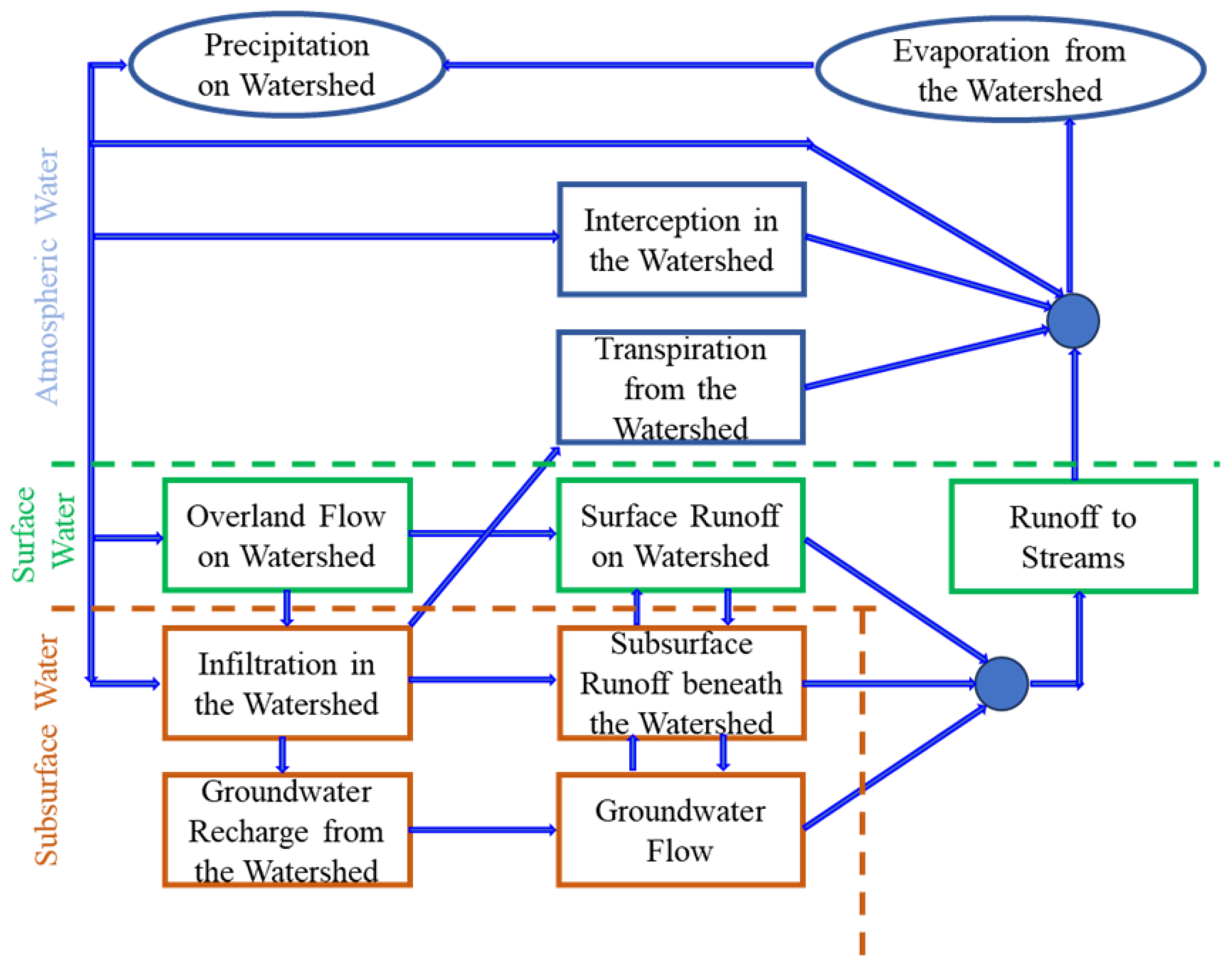
Figure 1. A flow chart to represent the hydrologic processes on watershed.
Eng 06 00129 g001
Figure 3. Radiation and heat balance in the atmosphere and at the Earth’s surface (see details in [1,14]).
Eng 06 00129 g003
Figure 4. Properties of vapor pressure, temperature, and raindrop.
Eng 06 00129 g004
Figure 5. Assumptions for measuring evaporation from an evaporation Pan and an open water surface (taken and modified from [1]).
Eng 06 00129 g005
Figure 6. Subsurface water zones and processes along with an unsaturated porous medium cross-section and the corresponding C V for the continuity equation (see details in [1]).
Eng 06 00129 g006
Figure 7. The moisture profile during infiltration, the infiltration rate (f), cumulative infiltration (F), parameters, and the soil column with a unit cross-sectional area based on the Green–Ampt infiltration model (see details in [1]).
Eng 06 00129 g007
Figure 8. Infiltration rate (f) and cumulative infiltration (F) for ponding under constant intensity rainfall.
Eng 06 00129 g008
Figure 9. Graphical representation of a unit hydrograph (a) and an example of discrete convolution (b).
Eng 06 00129 g009
Figure 10. Steps for selecting appropriate statistical tests for any study.
Eng 06 00129 g010
Figure 11. Mathematical modeling process, formulation, conceptual representation, and watershed model calibration.
Eng 06 00129 g011
Figure 12. Classification of watershed models.
Eng 06 00129 g012
Table 1. Summary of common probability distributions, their probability density functions, ranges, and parameters determined by sample moments.
DistributionPDFRangeParameter Equations
Normal f ( x ) = 1 σ 2 π e ( x μ ) 2 2 σ 2 x μ = x ¯ , σ = s x
Log-normal f ( x ) = 1 x σ 2 π e ( y μ y ) 2 2 σ y 2 x > 0 μ y = y ¯ , σ y = s y ; y = log x
Exponential f ( x ) = λ e λ x x 0 λ = 1 x ¯
Gamma f ( x ) = λ β x β 1 e ( λ x ) Γ ( β ) x 0 λ = x ¯ s x 2 , β = x ¯ 2 s x 2 = 1 C V 2
Pearson Type III f ( x ) = λ β ( x ϵ ) β 1 e ( λ ( x ϵ ) ) Γ ( β ) x ϵ λ = s x β ,   β = 4 C s 2 , ϵ = x ¯ s x β
Log Pearson Type III f ( x ) = λ β ( y ϵ ) β 1 e ( λ ( y ϵ ) ) Γ ( β ) y ϵ ; y = log x λ = s y β β = 4 C s ( y ) 2 , ϵ = y ¯ s y β
Extreme Value Type I f ( x ) = 1 α e x μ α e x μ α < x < α = 6 s x π , μ = x ¯ 0.5772 α
Table 2. Model types and examples of models.
Model TypeHydrologic Models
Lumped parameterSnyder or Clark UH
DistributedKinematic wave
EventHEC-1, HEC-HMS, SWMM, SCS TR-20
ContinuousStanford Model, SWMM, HSPF, STORM
Physically basedHEC-1, HEC-HMS, SWMM, HSPF
StochasticSynthetic streamflows
NumericalKinematic or dynamic wave models
AnalyticalRational Method, Nash IUH
Table 3. Models and their application areas.
ModelsApplication Areas
HEC-HMSDrainage, land use change impact on flooding
National Weather Service (NWS)Flood forecasting
Modular Modeling System (MMS)Water resource planning works
University of British Columbia (UBC) and WATFLOODHydrologic simulation
Runoff-Routing model (RORB) and WBNFlood, drainage, land use change impact
TOPMODEL and SHEHydrologic analysis
HBVFlow forecasting
Table 4. Comparative analysis across scales.
Criteria HSPF HEC - HMS SWAT MIKE SHE
Scale suitabilityMedium to largeSmall to mediumLargeSmall to large
Temporal scaleHourly to dailySub-hourly to dailyDailySub-hourly to daily
Spatial representationLumpedSemi-distributedSemi-distributedFully distributed
Data requirementHighModerateModerate to highVery high
User friendlinessModerateHighModerateLow
Enhanced modelingWater qualityHydrology onlySediment/nutrientIntegrated
Calibration computationComplexEasyModerateVery complex
Computational loadModerateLowModerateHigh
Disclaimer/Publisher’s Note: The statements, opinions and data contained in all publications are solely those of the individual author(s) and contributor(s) and not of MDPI and/or the editor(s). MDPI and/or the editor(s) disclaim responsibility for any injury to people or property resulting from any ideas, methods, instructions or products referred to in the content.