Article

Prediction of Key Parameters in the Design of CO2 Miscible Injection via the Application of Machine Learning Algorithms

1
Department of Mining and Petroleum Engineering, University of Boumerdes, Boumerdes 35000, Algeria
2
Department of Petroleum Engineering, University of North Dakota, Grand Forks, ND 58202, USA
3
Department of Energy and Petroleum Engineering, University of Wyoming, Laramie, WY 82072, USA
*
Author to whom correspondence should be addressed.
Eng 2023, 4(3), 1905-1932; https://doi.org/10.3390/eng4030108
Submission received: 2 June 2023 / Revised: 1 July 2023 / Accepted: 5 July 2023 / Published: 7 July 2023
(This article belongs to the Special Issue GeoEnergy Science and Engineering)

Abstract

:
The accurate determination of key parameters, including the CO2-hydrocarbon solubility ratio (Rs), interfacial tension (IFT), and minimum miscibility pressure (MMP), is vital for the success of CO2-enhanced oil recovery (CO2-EOR) projects. This study presents a robust machine learning framework that leverages deep neural networks (MLP-Adam), support vector regression (SVR-RBF) and extreme gradient boosting (XGBoost) algorithms to obtained accurate predictions of these critical parameters. The models are developed and validated using a comprehensive database compiled from previously published studies. Additionally, an in-depth analysis of various factors influencing the Rs, IFT, and MMP is conducted to enhance our understanding of their impacts. Compared to existing correlations and alternative machine learning models, our proposed framework not only exhibits lower calculation errors but also provides enhanced insights into the relationships among the influencing factors. The performance evaluation of the models using statistical indicators revealed impressive coefficients of determination of unseen data (0.9807 for dead oil solubility, 0.9835 for live oil solubility, 0.9931 for CO2-n-Alkane interfacial tension, and 0.9648 for minimum miscibility pressure). One notable advantage of our models is their ability to predict values while accommodating a wide range of inputs swiftly and accurately beyond the limitations of common correlations. The dataset employed in our study encompasses diverse data, spanning from heptane (C7) to eicosane (C20) in the IFT dataset, and MMP values ranging from 870 psi to 5500 psi, covering the entire application range of CO2-EOR. This innovative and robust approach presents a powerful tool for predicting crucial parameters in CO2-EOR projects, delivering superior accuracy, speed, and data diversity compared to those of the existing methods.

1. Introduction

As our modern society continues to hinge on oil for energy and a wide range of petrochemical products, ranging from everyday household goods to essential medicines, the management of oil resources has become increasingly critical [1]. Of particular concern are the diminishing recovery rates seen in oil fields worldwide, indicating that our current extraction techniques may not be sufficient to satisfy global demand [2]. Estimates suggest that more than half (about 2/3) of the original oil in place (OOIP) remains untapped after primary and secondary recovery methods are applied [3]. For instance, the Rhourde El Baguel (REB) field in Algeria has only managed to recover roughly 21% of the OOIP in over 30 years of production [4]. This points toward an urgent need for enhanced oil recovery (EOR) methods to retrieve substantial quantities of trapped oil [5].
The application of EOR is not just a matter of resource efficiency; it also plays a significant role in environmental preservation. As the oil and gas industry moves towards decarbonization in alignment with global efforts to mitigate climate change, the role of CO2-EOR becomes even more crucial as part of carbon capture, utilization, and storage (CCUS) strategies [6]. This approach aligns with the industry’s goal to remain a leading energy system while addressing environmental concerns. By effectively managing and utilizing CO2 emissions for oil recovery, the industry not only enhances its resource efficiency but also makes significant strides toward sustainability [7].
Among various EOR techniques, miscible CO2 gas injection has emerged as the most widely implemented approach in numerous countries, particularly for light oil reservoirs [8]. With nearly 80% of global reservoirs suited for some form of CO2 injection [9], this method’s growing prevalence can be attributed to the economic attractiveness of naturally sourced CO2, which provides a cost-effective supply [10].
The success of a CO2-EOR project heavily relies on key parameters such as minimum miscibility pressure (MMP), interfacial tension (IFT), and solubility (Rs) [11]. When CO2 is injected into oil reservoirs, it dissolves in the oil, causing the oil to swell and reducing its viscosity. This process also lowers the interfacial tension between fluid phases, aiding in the retrieval of trapped oil. Optimal conditions are achieved when the interfacial tension between fluid phases reaches zero, which signifies that CO2 has become fully miscible with the oil, thereby facilitating the most efficient oil displacement [12].
The oil and gas industry is currently undergoing a significant digital transformation, with advancements in artificial intelligence (AI) and machine learning reshaping traditional practices [13]. Machine learning is being leveraged for tasks such as analysis and modeling, drilling and subsurface characterization, forecasting maintenance requirements, optimizing supply chains, and financial resource management [14]. The integration of these technologies has seen a surge in recent years, and as the industry recognizes the value they add, innovative applications continue to multiply [15].
A substantial number of studies have sought to understand the EOR process via miscible CO2 injection, employing both experimental and numerical simulation techniques [16]. In recent times, machine learning methods have been increasingly used to gain valuable insights into EOR projects [15]. This study aims to further contribute to this burgeoning field by applying various supervised machine learning techniques to accurately predict key parameters including solubility (Rs), interfacial tension (IFT), and minimum miscibility pressure (MMP) required for effective CO2-EOR design.

2. Literature Review

The design of a CO2 miscible injection requires the prediction of key parameters such as the minimum miscibility pressure (MMP), CO2 solubility, and phase behavior of the CO2–oil system.
The minimum miscibility pressure (MMP) is a crucial parameter in CO2 miscible injection, as it indicates the pressure at which the injected CO2 and the oil become completely miscible [17]. Accurate prediction of the MMP is necessary to optimize the design of the CO2 injection process and increase oil recovery [18]. Several models and methods have been proposed to predict the MMP in CO2 miscible injection. These models can be categorized into equation of state (EOS) models and empirical models [19]. EOS models are based on the principle of thermodynamics and can predict the phase behavior of the CO2–oil system as a function of pressure and temperature. Empirical models, on the other hand, use statistical methods to fit experimental data and predict the MMP [20].
One of the most widely used EOS models for predicting the MMP is the Peng–Robinson (PR) equation of state. This model considers the interactions between the CO2 and oil molecules and it can predict the phase behavior of the CO2–oil system [21]. Several modifications have been proposed to improve the accuracy of the PR model for predicting the MMP. For instance, Kiani et al. [22] developed a new PR model that accounts for the impact of asphaltene on MMP prediction. This model was validated using experimental data and demonstrated superior accuracy compared to that of existing models. Additionally, Tahsin Ahmed [23] utilized a modified version of the PR EOS, along with a newly introduced “Miscibility Function”, to estimate the injection pressure required for miscible gas injection. Meanwhile, Alshuaibi et al. [24] developed a novel formula for the Abu Dhabi reservoir, which incorporates parameters such as temperature, saturation pressure, and reservoir fluid composition to determine the MMP. Rajak and Ashutosh [25] used multiple EOS models, despite the limited laboratory data, to develop a novel approach for estimating the appropriate MMP value. These methods offer potential ways to optimize the design of CO2 injection and enhance oil recovery.
Machine learning algorithms are another approach for predicting the MMP. Sinha et al. [26] developed an analytical correlation for calculating the MMP and tuned the correlation coefficients using linear SVM. They also used a hybrid approach that combined random forest (RF) regression and analytical correlation. Shakeel et al. [27] focused on artificial neural network (ANN) and adaptive neuro-fuzzy inference system (ANFIS) techniques to predict MMP for CO2 miscible flooding. The results showed that the ANN prediction was overall better than the ANFIS technique. Li et al. [28] evaluated the reliability of four machine learning-based prediction models including neural network analysis (NNA), genetic function approximation (GFA), multiple linear regression (MLR), and partial least squares (PLS) using 136 sets of data. Other machine learning models have also been developed for MMP prediction, such as those developed by the authors of [18,29,30,31,32].
The prediction of CO2 solubility in oil is another important parameter that affects the design of CO2 miscible injection. Various models have been developed to accurately predict CO2 solubility in crude oil. Zhang et al. [33] developed a novel method using artificial neural networks to predict CO2 solubility in heavy oil, which was found to be accurate and more efficient than traditional simulation methods. Dadan et al. [34] provided a reliable model to predict CO2 solubility in formation brines using ion-specific parameters and a binary interaction parameter between ions and CO2. The solubility of CO2 in aqueous electrolyte solutions was also described using the electrolyte perturbed hard-sphere chain equation of state (e-PHSC) by Dadan et al. [34]. Zhen et al. [35] employed an artificial neural network (ANN) and support vector machine (SVM) to develop GC models based on 10,116 CO2 solubility data measured in various ionic liquids (ILs) at different temperatures and pressures. These models can significantly aid in the design of a CO2 miscible injection.
The phase behavior of the CO2–oil system is another critical parameter that affects the design of a CO2 miscible injection. Cheng et al. [36] investigated the effect of phase behavior on the design of a CO2 miscible injection. The study showed that the CO2–oil system can exhibit different phase behaviors depending on the pressure and temperature conditions. Therefore, it is important to consider the phase behavior when designing CO2 miscible injection. Zhao et al. [37] developed a new model to predict the CO2–oil phase behavior using the Grayson–Streed method. The model was validated using experimental data and was found to be more accurate than existing models.

3. Data Collection

Data collection stands as the cornerstone in resolving any supervised machine learning problem. The efficacy of predictive models hinges largely on the quality of the data they are derived from. As such, meticulous data collection practices have become an indispensable component in crafting highly effective models. The collected data need to be free from errors and brimming with pertinent information directly relevant to the task at hand.
Before embarking on the journey of model development, we must subject our collected data to rigorous statistical analysis. This preliminary step ensures that we gauge the quality of data distribution, isolate and eliminate any outliers, and verify the presence of relationships among our parameters. This data-driven examination lays a solid groundwork for our subsequent machine learning endeavors, facilitating more accurate, reliable, and effective predictive modeling.

3.1. Solubility (Rs)

Our dataset for this study was gathered from various published research articles [38,39,40,41,42]. We used laboratory measurements of the solubility of carbon dioxide (CO2) in oil, taken with the experimental apparatus.
The primary inputs to our dataset were saturation pressure (Ps, MPa), bubble point pressure (Pb, MPa), temperature (T, °C), molecular weight (MW, gr/mol), and specific gravity (γ). We selected these parameters because they are critical to describing CO2 solubility. Furthermore, these properties are frequently utilized in artificial intelligence projects focusing on solubility.
By focusing on these parameters, we could accurately characterize CO2 solubility, ensuring that our dataset was relevant and precise. This selection also facilitated the effective development and execution of our machine learning models, allowing a meaningful analysis of the collected data. Table 1 shows a statistical description of the data.
A pair plot was executed for both datasets to visually represent the distribution and approximate density of each variable. It also enables us to observe the interrelation between these variables. The variations within each graph can be observed in Figure 1 displayed below.
The graphs are arranged in a matrix format, where the rows represent the y-axis and the columns represent the x-axis. The diagonal subplots display the individual distributions of each attribute. For instance, when examining the molecular weight distribution in dead oil, it is observed that the values are well-distributed and mostly fall within a range from 200 to approximately 490 gr/mol. The distribution density is higher between 350 and 375 gr/mol. Conversely, in live oil, the molecular weight values are relatively lower compared to those of dead oil, ranging between 13 and about 300 gr/mol. The distribution density is higher between 110 and 170 gr/mol. These molecular weight ranges align with the physical properties of the oils; live oil contains volatile components, resulting in a higher distribution density in the lower molecular weight range. On the other hand, dead oil is a heavier oil or residue that has lost its volatile components, leading to a higher distribution density in the higher molecular weight range.
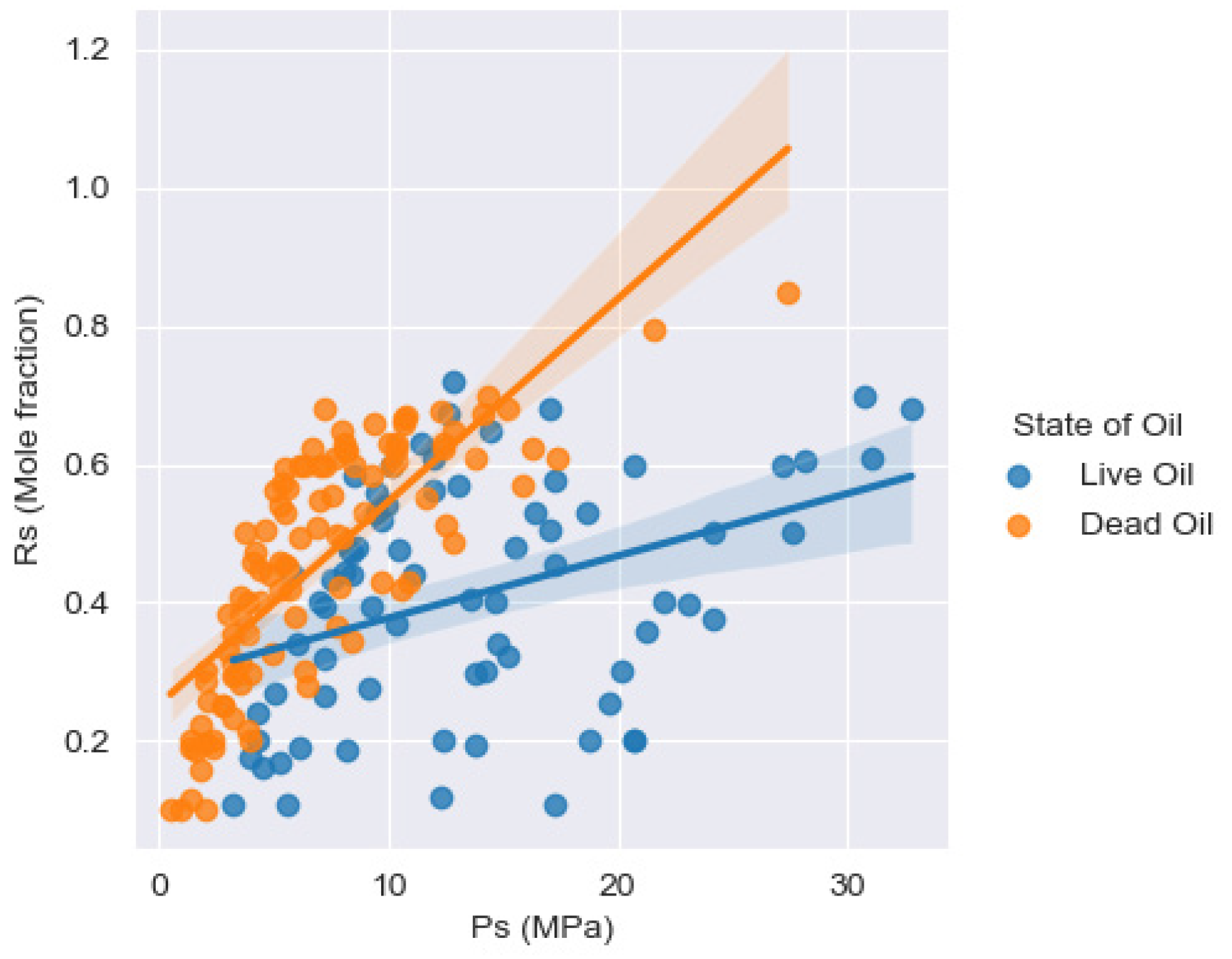
Furthermore, the graphs reveal a significant correlation between saturation pressure (Ps) and the solubility of CO2 (Rs) in both models. As the saturation pressure increases, the solubility also increases.
Figure 2 depicts a graph with linear curves, providing a clearer illustration of the strong relationship between these variables.
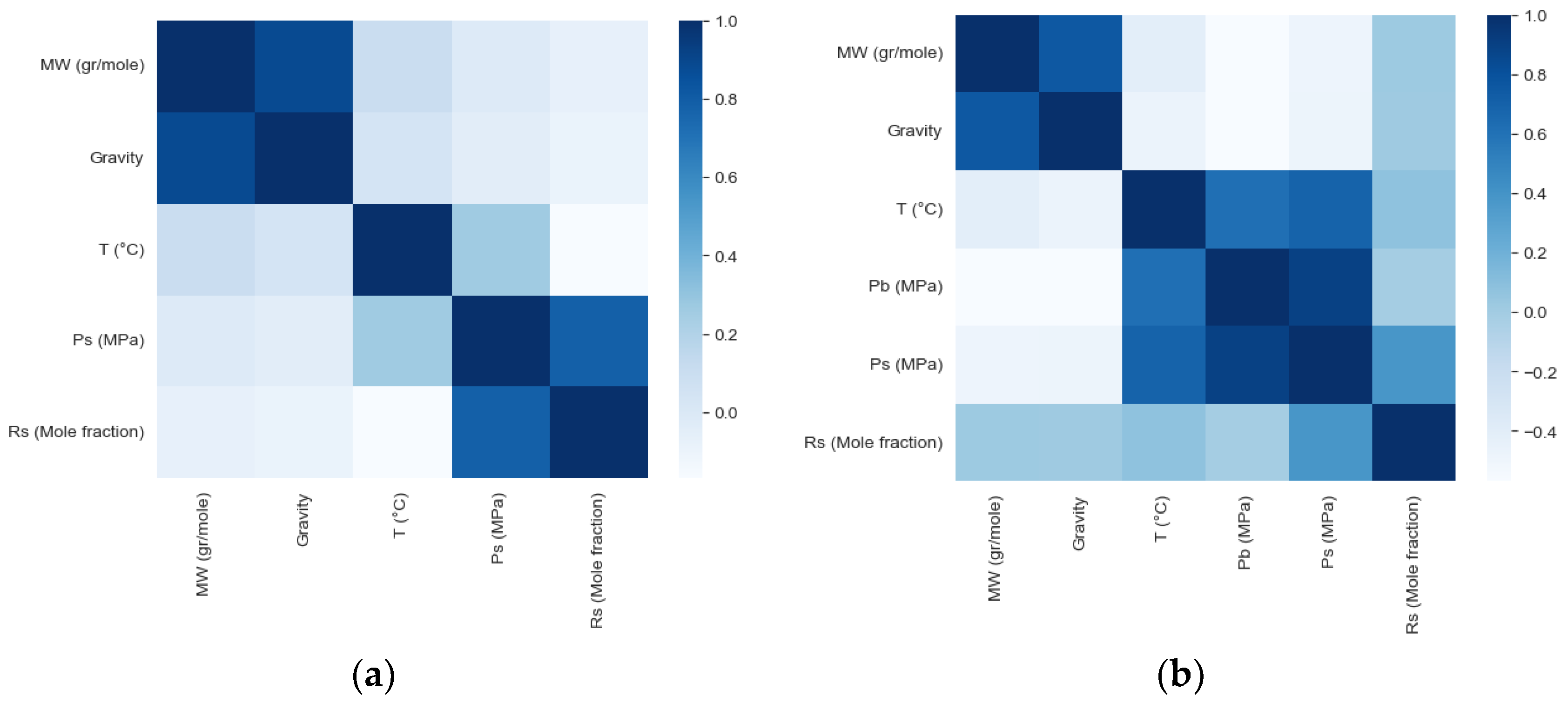
The Pearson correlation coefficient was employed to quantify the degree of association between the input variables and solubility, further validating the aforementioned observations. Table 2 and the heat maps in Figure 3 presented below depict the correlation coefficients for each parameter.
The heatmaps clearly indicate that certain input variables exhibit a weak linear relationship with solubility. This implies that a linear model may not be suitable for capturing these relationships effectively. Consequently, a nonlinear implementation is required to accurately identify and model these relationships.

3.2. Interfacial Tension (IFT)

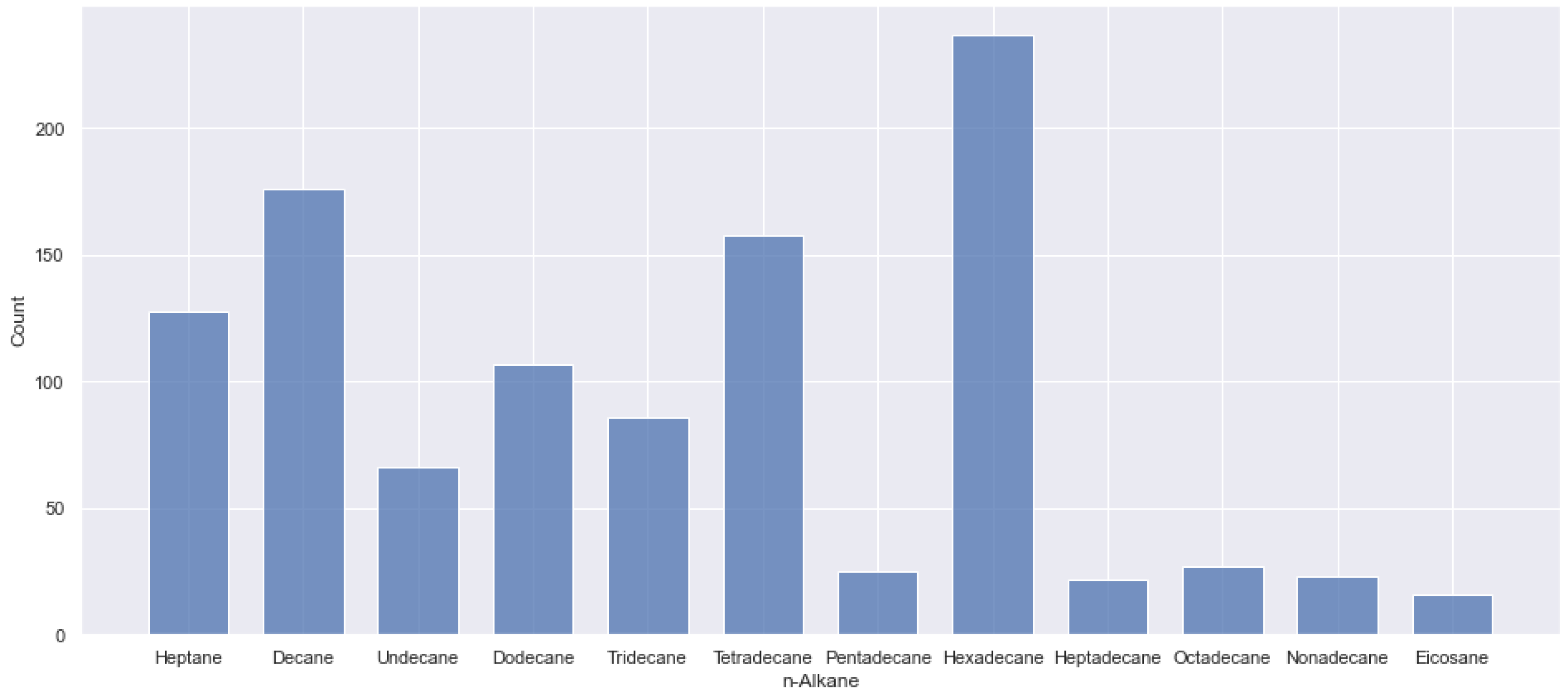
Data regarding CO2–n-alkane interfacial tension (IFT, mN/m) were gathered from various research sources, including works by Zolghadr et al. [43], Philip T. Jaeger [44], and Georgiadis et al. [45]. It is important to note that the sessile drop technique at high pressures was the primary method used for experimentally determining the interfacial tension in most of these sources. The histogram displayed below (Figure 4) illustrates the data distribution for each component.
The parameters that characterize the interfacial tension include pressure (P, MPa), temperature (T, K), molecular weight (MW, g/mol), critical temperature (Tc, K), critical pressure (Pc, MPa), and the acentric factor (ω) of the n-alkane. Table 3 provides a statistical description of the dataset. These properties were chosen because of their significant impact on interfacial tension, making them crucial inputs to our dataset. This careful selection of features ensured that our machine learning models were informed by relevant and precise data, leading to accurate and meaningful results.
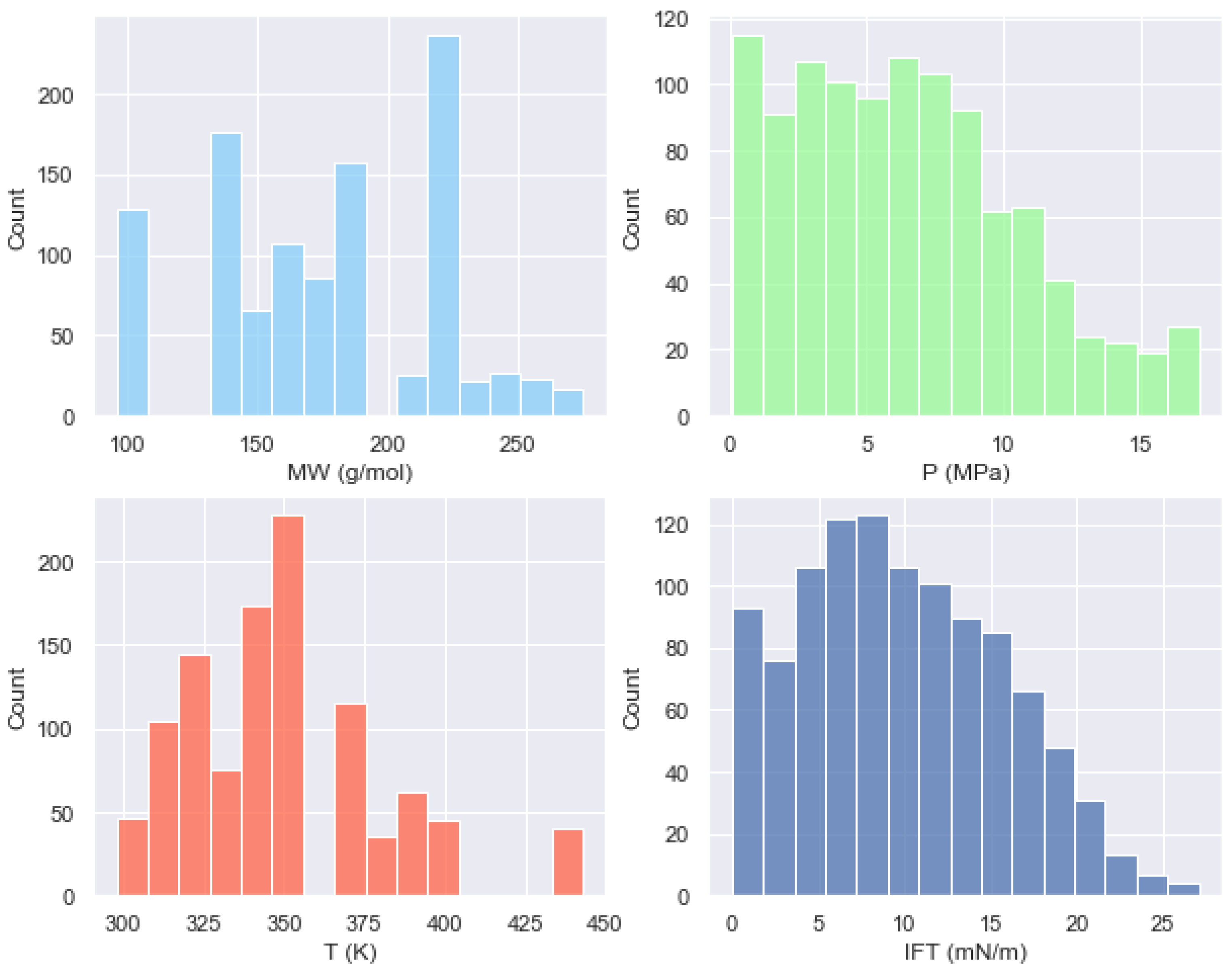
By examining the histograms presented in Figure 5, it is evident that the data for each parameter are distributed effectively within their minimum and maximum ranges. Taking molecular weight and pressure as examples, we observe a high-density distribution between 210 and 230 g/mol, particularly peaking at 222 g/mol, which corresponds to hexadecane. As for pressure, there is a notable concentration of values below 10 MPa. This is of particular interest because, for economic reasons, it is desirable to achieve low interfacial tension (IFT) values at the lowest possible pressure.
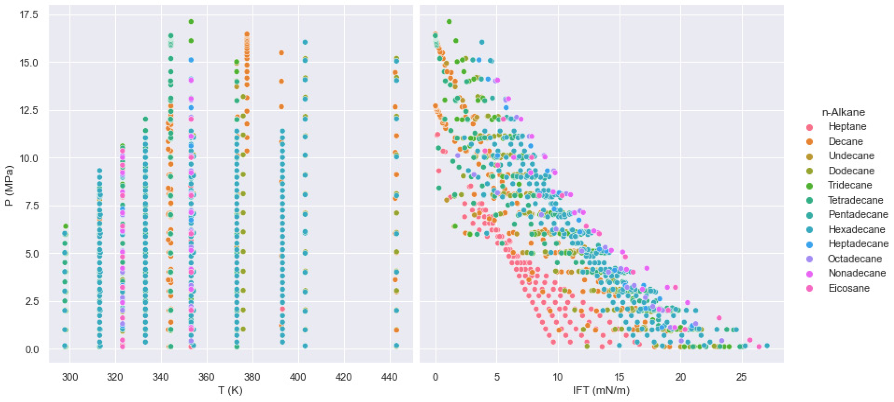
To gain deeper insights into the impact of pressure on interfacial tension, a scatter plot (Figure 6) was created to visualize the relationship between pressure and interfacial tension at different temperature values. The first graph demonstrates a uniform distribution of pressure for each temperature, reflecting the experimental principle outlined by the authors in the literature. The experimental method, known as the sessile drop technique, involves gradually increasing pressure to observe the behavior of interfacial tension across multiple temperature values (in this case, 11 values). The experiment was repeated with diverse compositions, and the results were recorded. In the second graph, a prominent association between interfacial tension (IFT) and pressure is evident. As pressure rises, there is a noticeable reduction in interfacial tension. This correlation holds true for all compositions tested, indicating the consistent influence of pressure on interfacial tension.
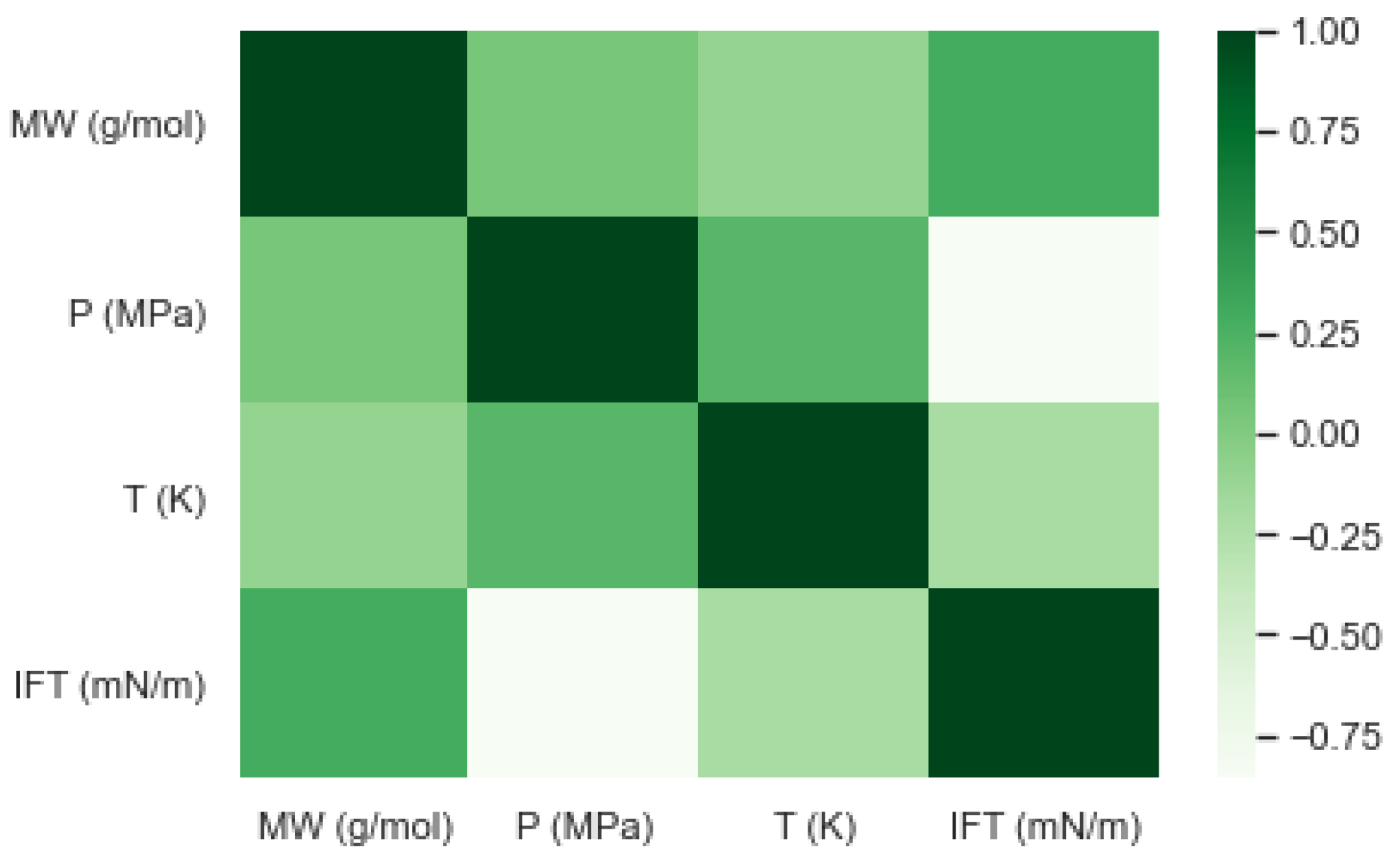
The correlation coefficients displayed in Table 4 and Figure 7 below reveal notable relationships between the variables. Pressure exhibits a strong negative correlation with interfacial tension, indicated by a coefficient of −0.8577. Similarly, temperature shows a negative correlation, albeit weaker, with a coefficient of −0.2042. Conversely, molecular weight displays a positive linear relationship with interfacial tension, reflected by a coefficient of 0.2918.

3.3. Minimum Miscibility Pressure (MMP)

The data utilized for the model’s development were obtained from various literature sources, notably Cronquist [46], Metcalfe [47], Alston et al. [48], Yuan et al. [49], and Zhang et al. [50]. Multiple slim tube tests were conducted under varying conditions, and the minimum miscibility pressure (MMP, MPa) values were recorded in each instance.
The key factors that influence the MMP are reservoir temperature, oil composition, and the components of the injected gas. Accordingly, the inputs chosen for our model included reservoir temperature (TR, K), the critical temperature of the injected gas (TC, K), an oil composition represented by a molecular weight of C5 and heavier (MWC5+, g/mol), and the ratio of volatile to intermediate components (xvol/xint). This selection of inputs ensured that our model was guided by factors directly influencing the MMP, providing a reliable basis for accurate predictions.
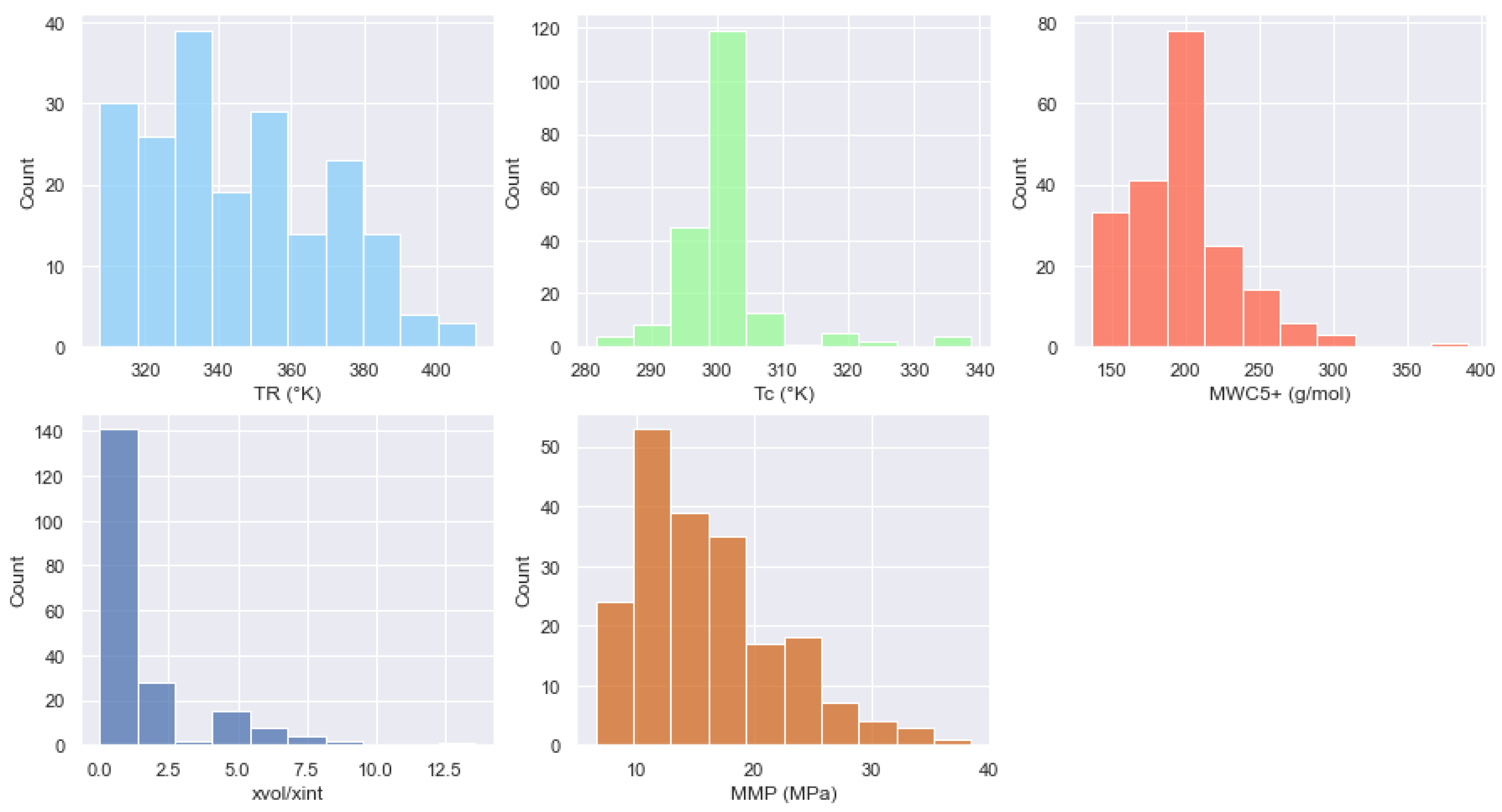
The histograms displayed in Figure 8 effectively visualize the distribution of the data, and Table 5 provides a statistical description of the MMP dataset.
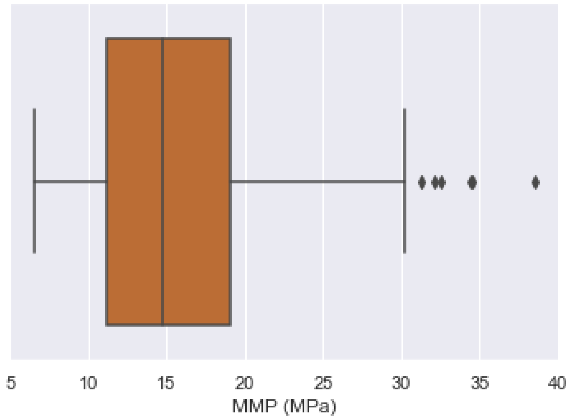
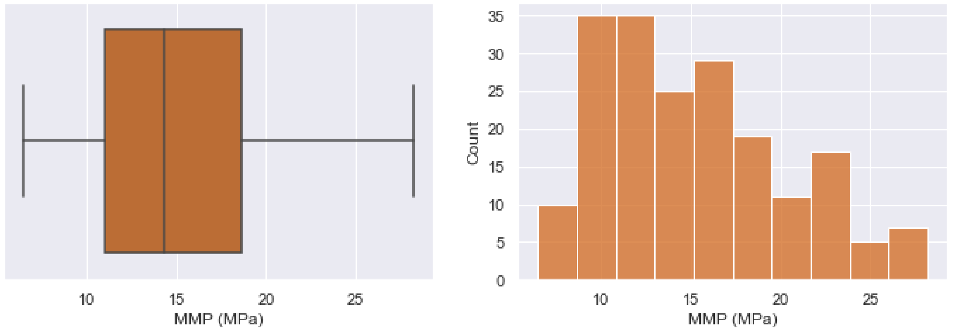
The histograms provide visual evidence that although the dataset covers a wide range of values, there are certain variables that are not well-distributed and may not be statistically significant. Taking MMP (minimum miscibility pressure) values as an example, we observe that the 75th percentile of the data is 19.12 MPa, while the maximum value reaches 38.52 MPa. Upon closer examination of the MMP histogram, it becomes apparent that only a small number of samples (six samples) fall above the 30 MPa threshold. To further validate and identify these values as outliers, boxplots serve as excellent visualization tools. They enable the identification of abnormal and outlier data points, which can aid in making informed decisions about their inclusion or exclusion from the dataset.
The box plot operates by identifying outliers as values that fall below the limit on the left (Q1 − 1.5 ∗ IQR) and above the limit on the right (Q3 + 1.5 ∗ IQR), where Q1 represents the first quartile (25th percentile), Q3 denotes the third quartile (75th percentile), and IQR corresponds to the interquartile range (the width of the box being from the 25th to 75th percentile). In Figure 9, the box plot reveals the presence of six outliers (represented by diamonds) that surpass the 30 MPa threshold, indicating the need for their removal from the dataset.
It is crucial to perform this step prior to model development to ensure optimal results, as retaining these outliers would likely lead to higher error values and a lower correlation coefficient. Attempting to train the model effectively with only six values above 30 MPa would be challenging. Figure 10 demonstrates the updated box plot visualizations and data distribution histogram after removing the outliers, enabling a more accurate representation of the dataset.
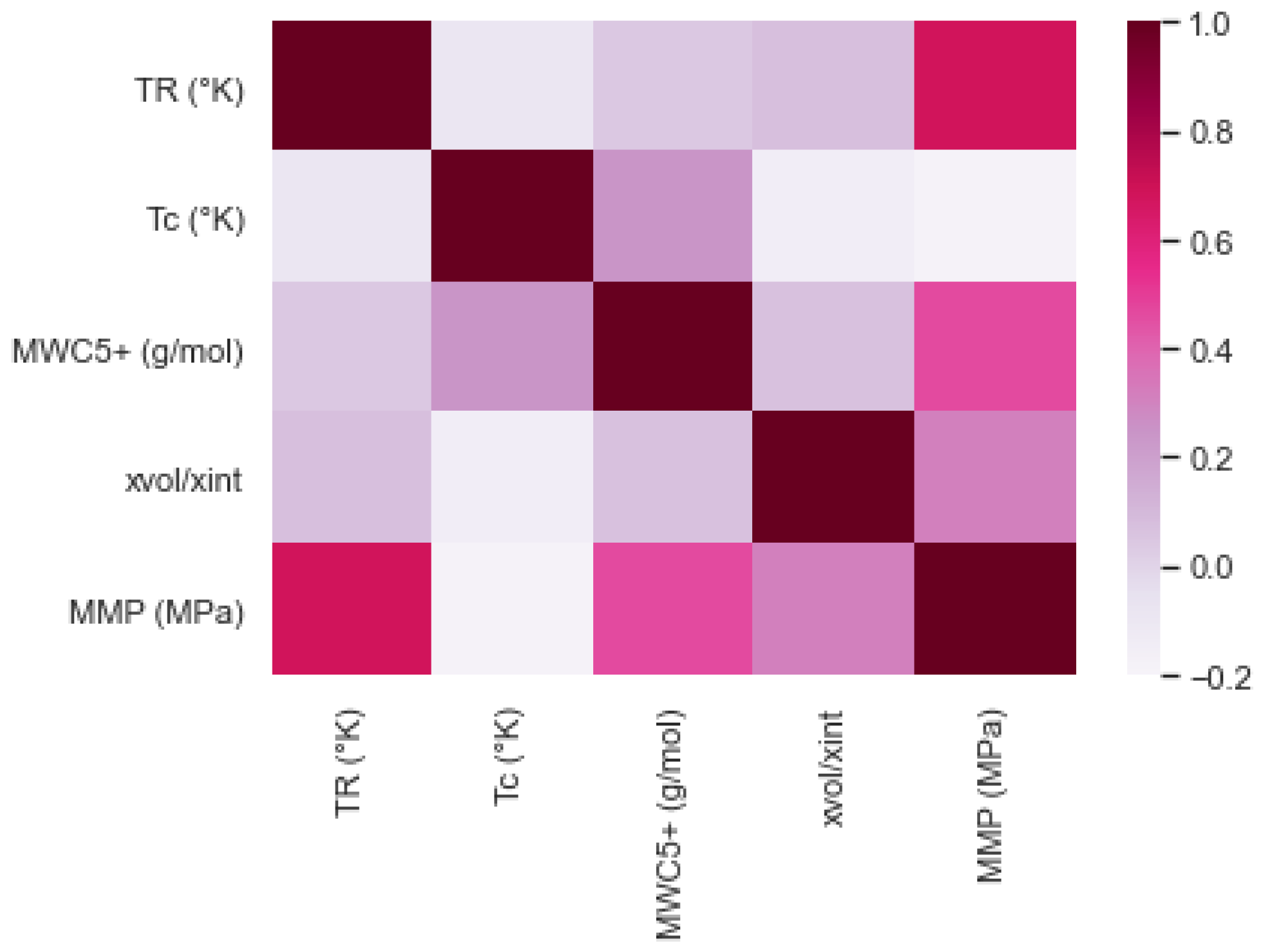
As depicted in Table 6 and Figure 11 below, a clear pattern emerges regarding the influence of various parameters on MMP variation. Reservoir temperature stands out as the most influential factor, displaying a strong positive correlation with a coefficient of 0.68. This indicates that as the temperature rises, the MMP tends to increase as well. Additionally, the molecular weight exhibits a moderate positive relationship with MMP, evident from its correlation coefficient of 0.47. Similarly, volatile to intermediate components show a modest positive correlation with a coefficient of 0.31. On the other hand, the critical temperature demonstrates a small negative linear relationship with the other parameters. Although this negative correlation is relatively weak, it still provides valuable insights and adds value to our predictive model.

4. Model Implementation

In the process of training machine learning models, it is often observed that the models might start to overfit or memorize the training data. While this might lead to good performance on the training set, it could also result in poor predictive accuracy for unseen data. To counteract overfitting and ensure the model’s generalization, the dataset is commonly partitioned. Thus, the datasets in this study were randomly divided into distinct subsets:
  • Dead oil solubility model: the training and validation set comprised 85% of the dataset (90 samples), and a test set formed 15% of the dataset (15 samples).
  • Live oil solubility model: the training set contained 80% of the dataset (60 samples), and a test set held 20% of the dataset (14 samples).
  • Interfacial tension model: the training set included 80% of the dataset (856 samples), a cross-validation set made up 1/8 of the training set (107 samples), and a test set represented 20% of the dataset (215 samples).
  • Minimum miscibility pressure model: the training set consisted of 84% of the dataset (162 samples), and a test set incorporated 16% of the dataset (31 samples).
In addition, normalization of data was conducted before inputting them into machine learning models to ensure consistent ranges. For example, in the case of solubility, the molecular weight values extended up to 490 gr/mol, while specific gravity values remained as less than 1. To balance this, z-score normalization was applied.
It should also be noted that Python 3.8 and its associated libraries were utilized for the development of all models.

4.1. Dead Oil Solubility

Initially, a multilayer perceptron (MLP) model was constructed, owing to its robust nonlinear representation capability, and its foundational unit being a neuron. The configuration of varying numbers of neurons and layers enables the characterization of mapping relationships of differing complexity levels. The inputs for this model were saturation pressure (Ps, MPa), temperature (T, °C), molecular weight (MW, gr/mol), and density (γ). As a result, a four-layer structure was established, with the input layer, two hidden layers, and an output layer, respectively containing 4, 12, and 1 neuron, as illustrated in Figure 12.
The flowchart presented in Figure 13 outlines the primary steps involved in constructing the MLP-Adam model and determining the optimal parameters that yield the lowest possible error. Appendix B provides a comprehensive overview of the feed forward equation in its general form, along with the corresponding weight and bias values. Additionally, it includes a detailed example illustrating the calculations using these specific weight and bias values. Table 7 provides details on the structure of the MLP-Adam model.
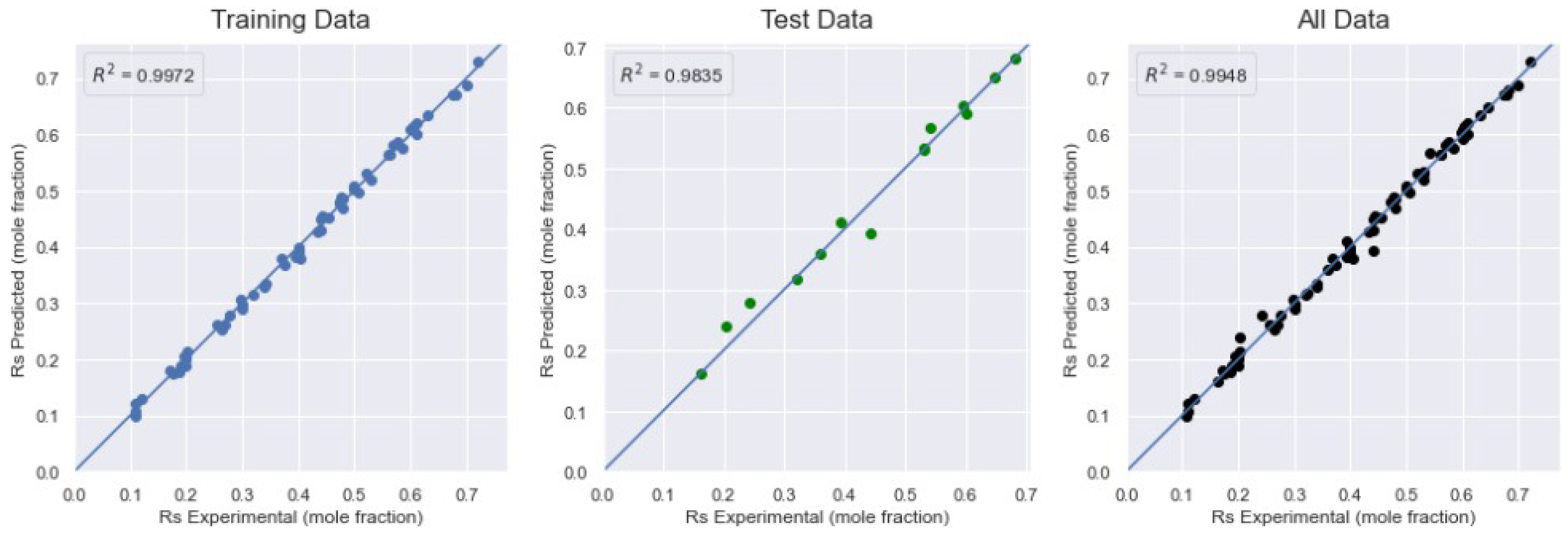
In order to evaluate the accuracy and predictive ability of the MLP-Adam model for Rs in dead oil, the average absolute relative deviation (AARD (%)), root mean square error (RMSE), and coefficient of determination (R2) were computed (please refer to Appendix A for the definition and mathematical formulation of these metrics). The outcomes of these calculations are presented in Table 8. For visual validation, the predicted values versus the actual values for both the training and test data are depicted in Figure 14.
The efficacy of the model was eventually benchmarked against some of the most commonly employed correlations in the field. The selected models from the literature include the Chung et al. [51] correlation, the Rostami et al. [52] correlation, and the genetic algorithm-based correlations of Emera and Sarma [53]. The comparative analysis was conducted utilizing the statistical parameters AARD (%), RMSE, and R2 (check Table 9)and supplemented with an error histogram plot of the different correlations as depicted in Figure 15 below. Upon examination, the histogram of Chung et al. showcases a significant error in comparison to the other models. While the model by Emera and Sarma holds a considerable number of zero-error values, its distribution is skewed to the right with a somewhat wide error range. The model from Rostami et al. [52] presents a favorable error distribution with minimal values; nevertheless, the MLP-Adam model is still considered superior in comparison to those outlined in the literature.

4.2. Live Oil Solubility

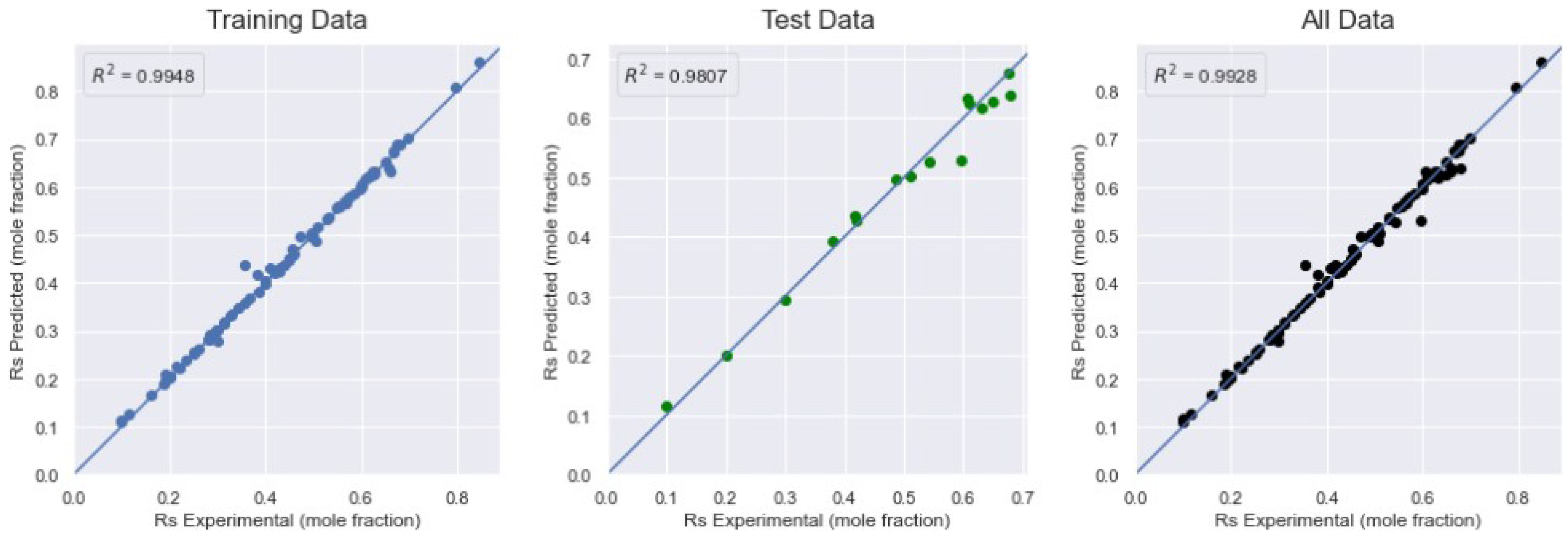
In the instance of live oil, a support vector regression (SVR) model was constructed, with the radial basis function (RBF) being selected as the kernel function in the SVR configuration. The selection of RBF over other kernel functions can be attributed to its lower number of parameters requiring optimization and reduced computational cost [54]. Of the 74 available samples, 60 were utilized for model construction, while the remaining data served to assess model performance. In this section, an additional input, bubble point pressure (Pb, MPa), was included alongside those employed in the dead oil model. To produce a model of high accuracy, it is crucial to ascertain the optimal values of the SVR-RBF hyperparameters. In this study, the grid search method was employed to identify these optimal values in a comprehensive manner. The search range for epsilon, gamma, and C, along with the corresponding optimal values yielded via the global search, are detailed in Table 10. In total, 30 support vectors were used to construct the decision function.
The solubility values forecasted by the SVR-RBF model are plotted with the empirically determined solubility values, encompassing the training data, test data, and the complete dataset, in Figure 16. Subsequently, the statistical parameters AARD (%), RMSE, and R2 were computed, with the corresponding results presented in Table 11.
Finally, the process implemented for the dead oil model was replicated. The performance of the SVR-RBF model was benchmarked against the most prevalent correlations in the literature, with the comparison based on previously described statistical parameters, as shown in Table 12. To bolster this comparison, an error histogram was produced, visualizing the different correlations, as depicted in Figure 17.
Upon scrutinizing the table along with the distributions and ranges of the histograms, it becomes apparent that the SVR-RBF model outperformed the processed correlations, considering its error range and the amount of values with exceedingly low error. Nonetheless, the model proposed by Rostami et al. [52] demonstrated satisfactory accuracy when compared to the models of Chung et al. [51] and Emera and Sarma [53].

4.3. Interfacial Tension

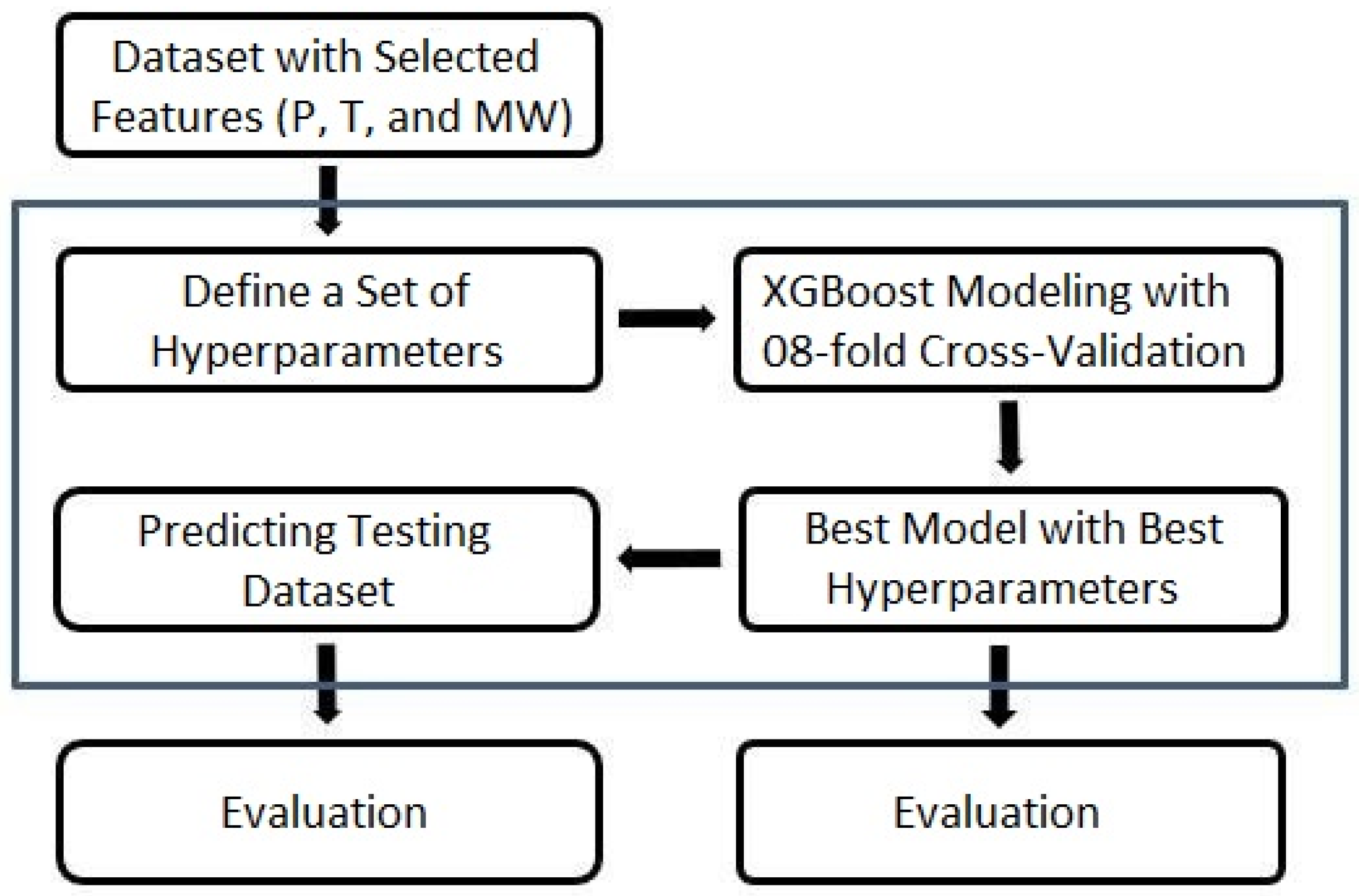
To construct a robust model adept at handling extensive datasets, an XGBoost model was employed, based on the decision tree approach. An 8-fold cross-validation scheme was utilized on the input set to evade the selection bias associated with training and testing data. The hyperparameters of XGBoost that delivered optimal performance are listed in Table 13. The main procedures in the construction of the model are outlined in the accompanying flowchart of Figure 18.
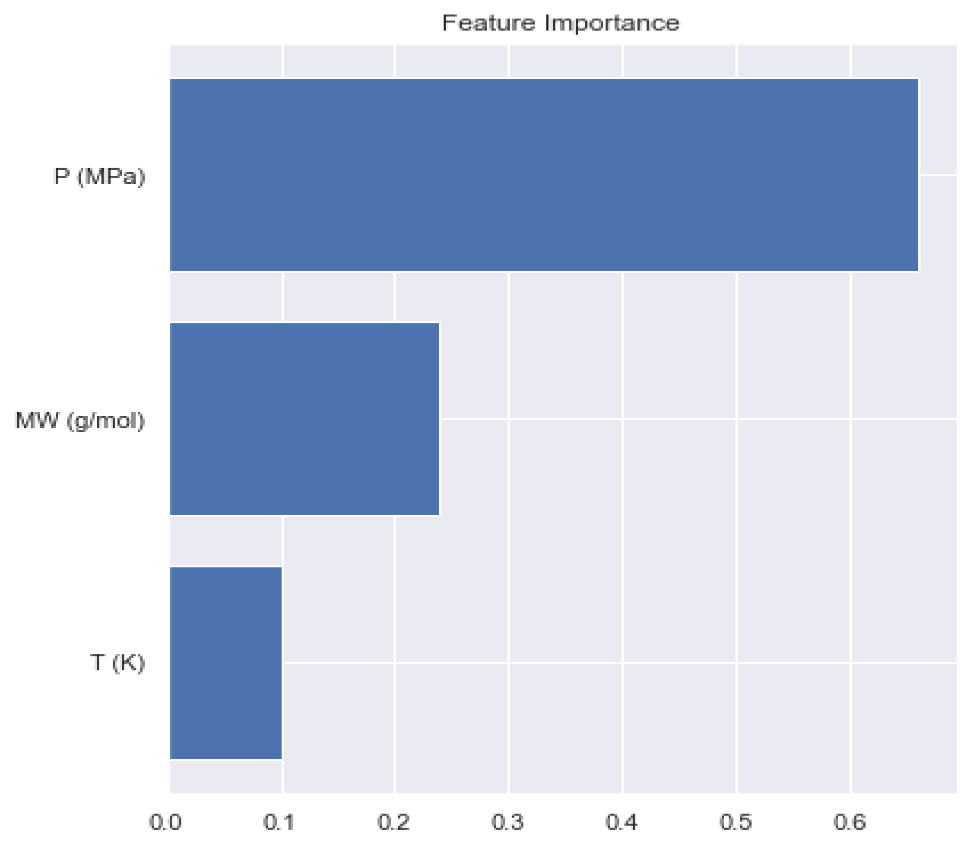
To obtain an understanding of the model’s decision-making process, and to discern which parameters held the most and least significance during prediction, the XGBoost model offers a remarkable feature that enables the visualization of parameter importance. This feature is demonstrated in Figure 19 below.
The interfacial tension values, predicted by the XGBoost model, are plotted against the corresponding experimentally measured values for the training set, the test set, and the entire dataset in Figure 20. The associated average absolute relative deviation (AARD (%)), root mean square error (RMSE), and coefficient of determination (R2) were computed and the resulting performance are provided in Table 14.
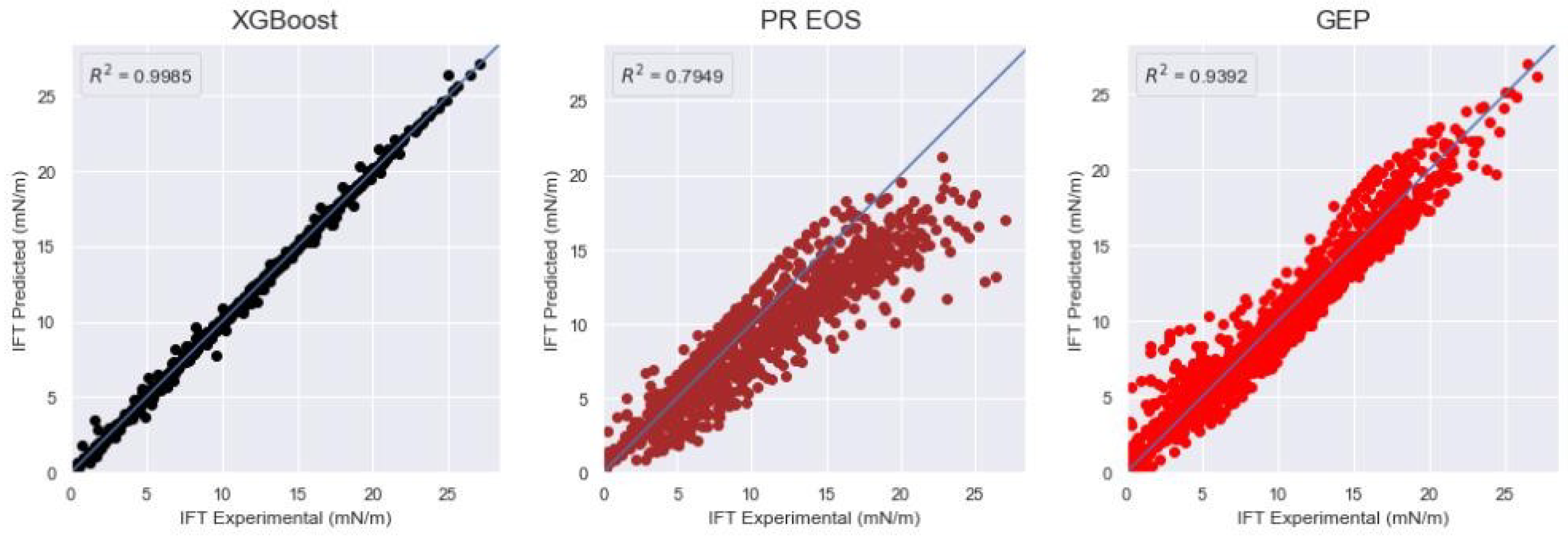
Ultimately, the reliability of the model was evaluated through a comparison of its predictive accuracy with the Peng–Robinson equation of state (PR EOS) and the GEP model put forward by Mirzaie et al. [55]. This comparative analysis was performed using the statistical parameters AARD (%), RMSE, and R2 (refer to Table 15), as well as through the construction of scatter plots that juxtapose the experimental IFT values with the respective predictions made by each model (see Figure 21).
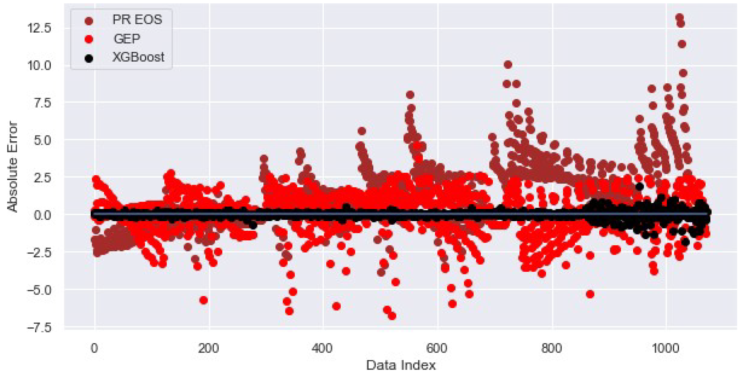
The equation-of-state model delivered satisfactory results for IFT < 15 mN/m, and the GEP model demonstrated its predictive efficacy across all data with an accuracy of 94%. However, the XGBoost model ultimately emerged as superior, boasting outstanding statistical parameters in comparison to the models currently available in the literature. Figure 22 depicts the absolute discrepancy between the experimental and predicted IFT values for the XGBoost, GEP, and EOS models. It’s evident that the XGBoost model displays the most minimal error values among the three, ranging from −2 to 2 with most values hovering around zero. On the other hand, the other models exhibit error values reaching up to 12.5 and lack a normal distribution of errors centered around zero.

4.4. Minimum Miscibility Pressure

XGBoost is used again on the MMP data, and it gave excellent prediction performance. The hyperparameters that fit the model best are shown in Table 16.
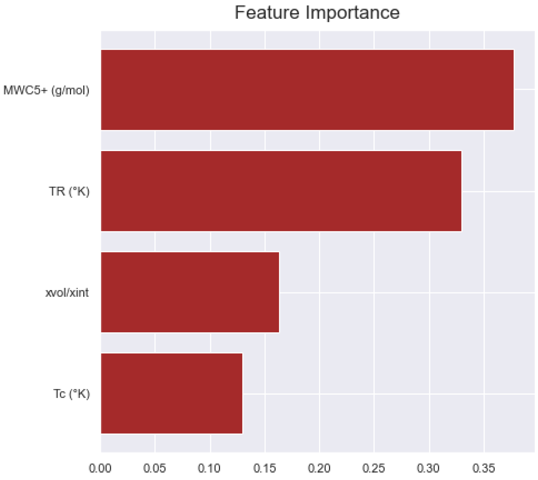
Following the approach adopted for the preceding IFT model, the significance of parameters for the MMP model is assessed, pinpointing those of utmost and least importance, as depicted in Figure 23. It’s readily apparent that the molecular weight of C5 plus stands out as the most significant variable, contributing 37.76%, followed by reservoir temperature at 32.93%, the ratio of intermediate to volatile components at 16.36%, and finally the critical temperature with 12.95%.
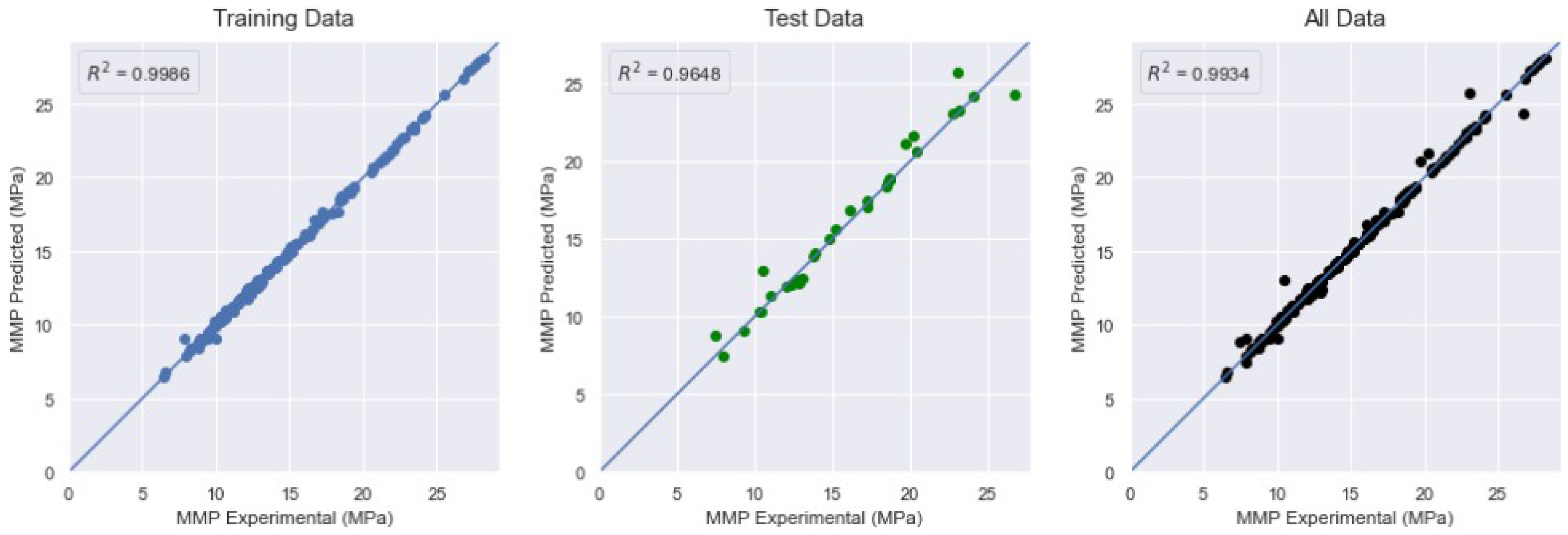
The XGBoost model’s predicted minimum miscibility pressure values are graphed against the experimentally determined values for the training data, the test data, and the complete dataset in Figure 24. Statistical metrics-average absolute relative deviation (AARD (%)), root mean square error (RMSE), and coefficient of determination (R2)-were computed, and the results are presented in Table 17.
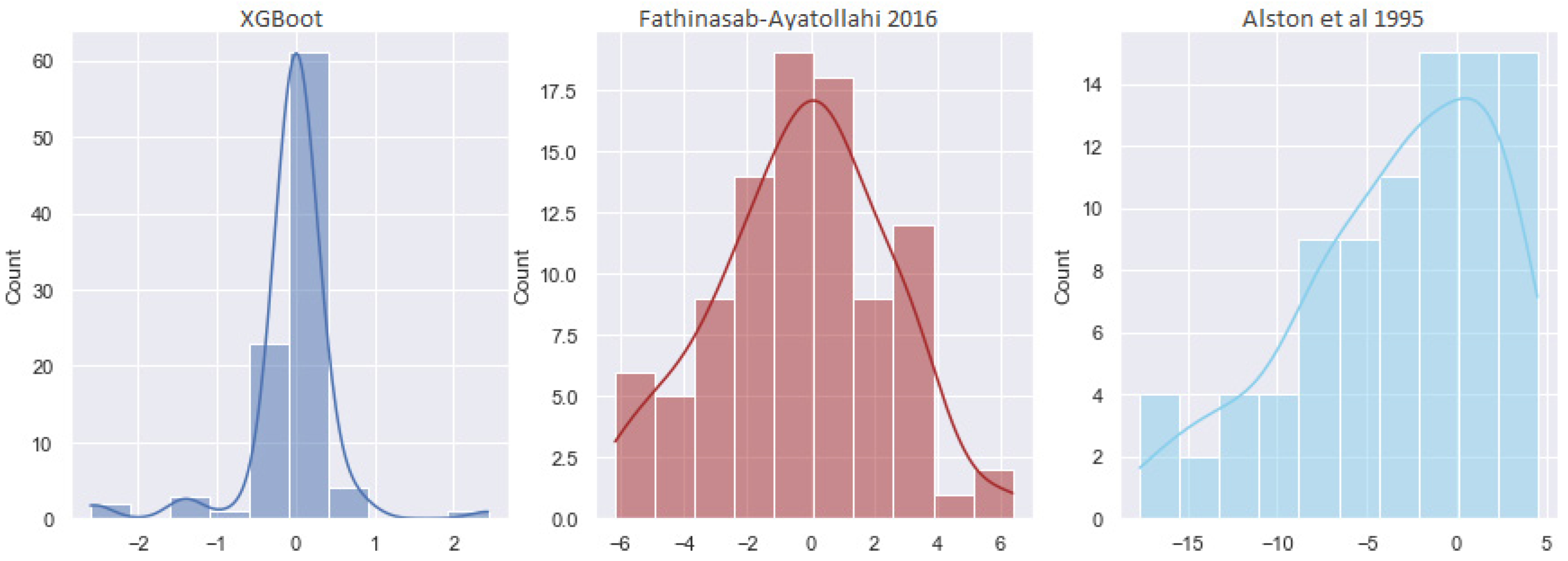
Upon completion of the evaluation process, the proposed model was compared to the most prevalent correlations in existing literature. Given the existence of specific correlations for pure CO2 (100% CO2) and others for impure CO2 (CO2 containing percentages of C1, N2, H2S, etc.), the data was bifurcated into ‘pure’ and ‘impure’ based on the critical temperature. For pure CO2, the correlations of Alston et al. (pure) [48], Lee [56], and Emera-Sarma [57] were used, while for impure CO2, the correlations of Alston et al. (impure) [48] and Fathinasab-Ayatollahi [58] were utilized. Table 18 summarizes the results of the comparison.
As can be seen in the aforementioned table, both the pure and impure XGBoost models exhibit the lowest AARD (%) and RMSE values, along with the highest coefficient of determination in comparison to the other models. Upon scrutinizing the error histograms for the pure CO2 case (Figure 25), it becomes apparent that while all correlations reasonably predict an acceptable quantity of values (roughly 20), they are subject to extensive error ranges and less satisfactory distributions when compared to the XGBoost model. The XGBoost model stands out with more than 50 values concentrated around 0, and an error range restricted to −1 to 0.5. This stark contrast emphasizes the superior performance and reliability of the XGBoost model when handling pure data.
In the scenario involving impure CO2 (Figure 26), the Fathinasab-Ayatollahi [58] correlation delivered a relatively low error margin and a fairly decent distribution compared to that of Alston et al. [48]. However, it still could not rival the predictive efficiency of the XGBoost model, which exhibited a minimal error margin ranging from −2 to 2 and recorded over 60 values clustered around 0. This further emphasizes the robustness and precision of the XGBoost model in estimating impure CO2 data.

5. Conclusions

This study introduces efficient and reliable models for estimating key parameters in CO2-enhanced oil recovery (CO2-EOR) operations: the solubility of CO2 in both dead and live oil, the interfacial tension, and the minimum miscibility pressure. These parameters are critical as they play a significant role in the planning and implementation of CO2-EOR projects. For instance, accurate estimation of the CO2 solubility in oil can inform on oil displacement efficiency, while a precise calculation of interfacial tension aids in assessing the mobility of the injected CO2, and understanding the minimum miscibility pressure is essential for the economic feasibility of the operation.
Our models, based on advanced machine learning algorithms—MLP, SVR, and XGBoost—and Adam’s optimization algorithm, present an innovative approach to estimate these parameters. They not only offer a high degree of precision and reliability but also showed a promising improvement over the existing correlations in the tests conducted.
However, it is worth mentioning that the real-world validation of these models in CO2-EOR projects remains an area for future exploration. Potential variability in the underlying data is another factor that could influence the models’ performance.
We recommend future work to focus on validating these models under diverse real-world conditions, and to explore emerging machine learning algorithms and optimization techniques for potential improvements. Such research directions can further enhance the planning and implementation of CO2-EOR projects, contributing to the advancements in the field of petroleum reservoir studies.

Author Contributions

Methodology, M.H., T.E.M. and N.Z.; Validation, A.L. and N.Z.; Investigation, M.H. and T.E.M.; Data curation, M.H. and T.E.M.; Writing–original draft, M.H., T.E.M. and A.D.; Writing–review & editing, A.L., O.S.T. and H.O. All authors have read and agreed to the published version of the manuscript.

Funding

This research received no external funding.

Data Availability Statement

The data presented in this study are available in the different articles declared in each section of the manuscript.

Conflicts of Interest

The authors declare no conflict of interest.

Appendix A

In this section, we present the definitions and mathematical formulas of the three metrics used to evaluate the models in this work.

Appendix A.1. Average Absolute Relative Deviation (AARD (%))

This is a measure of prediction accuracy in statistical modeling and forecasting. The AARD is expressed as a percentage, and lower values generally indicate better predictive accuracy. It is calculated as the average of absolute errors relative to the actual values.
The formula to calculate AARD is as follows:
A A R D   ( % ) = ( 1 n ) ( | A c t u a l P r e d i c t e d | ) A c t u a l   *   100
where
  • n is the total number of observations;
  • Actual refers to the actual value;
  • Predicted refers to the predicted value.

Appendix A.2. Root Mean Square Error (RMSE)

This is a standard way to measure the error of a model in predicting quantitative data. RMSE is essentially the standard deviation of the residuals (prediction errors). Lower values of RMSE indicate a better fit of the data. The formula for calculating RMSE is as follows:
R M S E = [ ( 1 n ) ( A c t u a l P r e d i c t e d ) 2 ]
where:
  • n is the total number of observations;
  • Actual refers to the actual value;
  • Predicted refers to the predicted value.

Appendix A.3. Coefficient of Determination (R2)

This is a statistical measure that represents the proportion of the variance for a dependent variable that is explained by an independent variable or variables in a regression model. So, if the R2 of a model is 0.50, then approximately half of the observed variation can be explained by the model’s inputs.
The formula for calculating R2 is as follows:
R 2 = 1 ( S S r e s     S S t o t )
where:
  • SSres is the sum of squares of the residual errors.
  • SStot is the total sum of squares.

Appendix B

In this section, we present the derivation of the feed forward equation for our proposed MLP-Adam model. The feed forward equation describes the mathematical relationship between the input features, hidden layers, and output prediction. Additionally, we provide tables of the weight and bias values for each layer, as well as an example calculation for a specific set of input features.

Appendix B.1. Feed Forward Equation of our MLP-Adam Model

Below is the step-by-step process of forwarding the input data through the layers of the network to generate the final output.
  • Initialize the input data. Let us denote the input vector as X.
  • Calculate the activations of the neurons in the first hidden layer by applying the ReLU activation function (this function computes the maximum value between 0 and the input x. If x is positive, the output is equal to x, and if x is negative, the output is set to 0) to the resulting sum to introduce non-linearity. This is carried out using the following equation:
    a 1 j = f ( z 1 j ) = R e L U ( i = 1 n w j i · X i + b j )
    where w j i is the interconnection weight between the input vector X i and the hidden layer neurons, j, z 1 j is the sum of the weighted inputs and the bias, b j , and n is the number of neurons in the input layer. a 1 j represents the resulting activation value.
3.
The same process is repeated for the second hidden layer. The output of the second hidden layer is denoted as a 2 .
a 2 k = f ( z 2 k ) = R e L U ( k = 1 p w j k · a 1 j + b k )
where w j k represents the weights connecting the first hidden layer neurons j to the second hidden layer neurons k, z 2 k Represents the weighted sum of inputs for the neurons in the second hidden layer, and b k is the bias term. a 2 k represents the activation values for this second hidden layer.
4.
Finally, the output of our MLP-Adam model can be calculated by applying the purelin function to the output of the ReLU function as shown below:
Y P = k = 1 p w k l · a 2 k + b l
where Y P is the predicted output value, w k l represents the weights connecting the second hidden layer neurons, k, to the output layer neurons, l, b l is the bias term, and p is the number of neurons in the hidden layer.
The combination of Equations (A4)–(A6) yields the following general form of the proposed neural network model:
R S = k = 1 p w k l · R e L U ( k = 1 p w j k   R e L U ( w j , 1 · M W + w j , 2 · γ + w j , 3 · T + w j , 4 · P s + b j ) + b k ) + b l
The values of the weights and biases are listed in Table A1 and Table A2 below.

Appendix B.2. Example Calculations using MLP-Adam Model

The example calculation uses the following values for the four input variables: MW = 490 gr/mol, γ = 0.967786, T = 140 °C, and Ps = 10.48 MPa. These values are utilized in the MLP-Adam model to derive the corresponding output prediction. The values were normalized using z-score normalization, which involved applying the following formula to each value:
X i s t d = X i μ σ  
where X i s t d represents the standardized value of a specific data point, X i denotes the original value of that data point, μ is the mean of the input data points, and σ is the standard deviation of the input data points. The normalized values of MW, γ, T, and Ps are 1.54606763, 0.90499909, 2.66878506, and 0.76176893, respectively.
By applying Equations (A4)–(A6), the predicted output is computed. The step-by-step calculations are outlined in Table A3, providing a comprehensive overview of the process.
Table A1. Weights and biases of the first hidden layer of the proposed MLP-Adam model.
w j ,   M W w j ,   γ w j ,   T w j ,   P s b j
0.423479229−0.5182706710.0888411400.164605036−0.182387754
−0.3168501550.578180193−0.627018213−0.370452255−0.037461437
−0.2609300610.1210959330.3026095620.1773411180.035739433
0.153113961−0.2736562780.023316100−0.014185284−0.152793422
0.3267218470.1635997140.0171128990.437370806−0.370236605
0.467836350−0.183758318−0.1163764960.1738477640.190825283
0.207402825−0.4029029600.2770750220.077882327−0.256408870
0.4306668340.4888470170.3824163070.316209614−0.437328159
−0.378489106−0.191637143−0.5867776270.073175244−0.207403078
−0.280519455−0.169934719−0.0386832200.4647877810.129119664
−0.012112551−0.2799097000.314301490−0.5536063310.127572730
0.2039907270.3480369440.120888933−0.571946859−0.362548828
Table A2. Weights and biases of the second hidden layer and the output layer of the proposed MLP-Adam model.
w 1 , k w 2 , k w 3 , k w 4 , k w 5 , k w 6 , k w 7 , k w 8 , k
0.1444445400.227294683−0.281868785−0.386379957−0.2449695610.250844776−0.0420569440.090741582
−1.246394872−0.613879323−0.8062542670.3329790830.174128487−0.160888448−0.9050390120.223389938
0.1583179380.1366026250.250266492−0.048559281−0.043032091−0.0094955120.364784896−0.316569924
−0.2921028730.0492416170.1139463930.185241475−0.1895625440.4732605810.171075671−0.035240747
−0.311310201−1.128083109−0.132358402−0.1476013800.150322437−0.051223963−0.0597101070.302232533
−0.5273177620.004510418−0.0907775980.0337730340.0035246070.325446367−0.200799241−1.144739747
0.641047120−0.0643884090.391169577−0.684768438−0.4347648910.371954649−0.063837923−0.090706437
−0.1906234620.2576516560.3940925890.200460493−0.2008687850.0645831370.1551789930.315470844
0.193483933−0.3017868100.255001187−0.513664782−0.427212923−0.234824061−0.0422430520.111917041
−1.0806194540.0968600950.1295109390.0498827580.238265812−1.2729544630.236488863−0.735467910
−0.364739000−0.515439033−0.178362324−0.179078683−0.595661461−0.054487861−0.096768409−0.003158351
−0.4999536870.379382699−0.177857115−0.423149019−0.9380390040.343048214−0.9564863440.245499372
w 9 , k w 10 , k w 11 , k w 12 , k b k w k , l b l
−0.792608916−0.343328714−0.205415770−0.5392004840.1585806900.0792467890.300516456
0.365020424−0.149115592−0.4261003130.1304894380.1239227130.187488675
0.1375885750.520926713−0.278029352−0.333180844−0.322128087−0.186551764
0.1918706140.492062687−0.308154106−0.2051180450.2592331760.440697550
−0.230481609−0.7262626880.058385573−0.124779440−0.0231452710.217374727
0.3793002960.1621331570.5671644210.756009399−0.201348185−0.275265455
−0.6337665310.0624757370.018612951−0.7102031700.1970994910.088092155
0.158039510−0.1239293660.0115500340.471806019−0.221232160−0.171224877
0.196399033−0.388778716−0.5686553120.230788096−0.103322580−0.453178435
0.274261921−0.6407087440.1553153840.2508342260.017402615−0.166323795
0.512196242−0.019978577−0.3306871650.1776317500.0798442280.371093213
−0.2564390890.436899453−0.4052977560.383212924−0.0868181880.109248526
Table A3. Example calculation using the proposed MLP-Adam Model.
MWγTPs z 1 a 1 z 2 a 2 Rs-PredRs-Exp
1.546067630.904999092.668785060.761768930.3657942
−1.9596565
0.68460845
−0.1123078
0.6618012
0.56967878
0.49840513
1.93238358
−2.4762450
−0.2075494
0.2726109
0.15474298
0.3657942
0
0.68460845
0
0.6618012
0.56967878
0.49840513
1.93238358
0
0
0.2726109
0.15474298
0.01417779
−0.9757543
−0.6840449
0.2759657
0.39354511
−2.3092059
0.31163391
0.64580446
−0.1985719
−2.0788913
−0.7179282
−0.8703367
0.01417779
0
0
0.2759657
0.39354511
0
0.31163391
0.64580446
0
0
0
0
0.42567880.42

References

  1. Holdren, J.P. Population and the energy problem. Popul. Env. 1991, 12, 231–255. [Google Scholar] [CrossRef]
  2. Laherrere, J.; Hall, C.B.; Bentley, R. How much oil remains for the world to produce? Comparing assessment methods, and separating fact from fiction. Curr. Res. Environ. Sustain. 2022, 4, 100174. [Google Scholar] [CrossRef]
  3. Ozotta, O.; Ostadhassan, M.; Lee, H.; Pu, H.; Kolawole, O.; Malki, M.L. Time-dependent Impact of CO2-shale Interaction on CO2 Storage Potential. In Proceedings of the 15th Greenhouse Gas Control Technologies Conference, Abu Dhabi, United Arab Emirates, 18 March 2021; pp. 15–18. [Google Scholar]
  4. Clonts, M.; Mazighi, M.; Touami, M. Reservoir simulation of the planned miscible gas injection project at Rhourde El Baguel, Algeria. In Proceedings of the European Petroleum Conference, Milan, Italy, 22–24 October 1996; OnePetro: Richardson, TX, USA, 1996. [Google Scholar]
  5. Malki, M.L.; Rasouli, V.; Saberi, M.R.; Sennaoui, B.; Ozotta, O.; Chellal, H.A. Effect of CO2 on Mineralogy, Fluid, and Elastic Properties in Middle Bakken Formation Using Rock Physics Modeling. In Proceedings of the ARMA US Rock Mechanics/Geomechanics Symposium, Santa Fe, NM, USA, 26–29 June 2022. [Google Scholar] [CrossRef]
  6. Hasan, M.M.F.; First, E.L.; Boukouvala, F.; Floudas, C.A. A multi-scale framework for CO2 capture, utilization, and sequestration: CCUS and CCU. Comput. Chem. Eng. 2015, 81, 2–21. [Google Scholar] [CrossRef] [Green Version]
  7. Merzoug, A.; Mouedden, N.; Rasouli, V.; Damjanac, B. Simulation of Proppant Placement Efficiency at the Intersection of Induced and Natural Fractures. In Proceedings of the ARMA US Rock Mechanics/Geomechanics Symposium, Santa Fe, NM, USA, 26–29 June 2022. [Google Scholar] [CrossRef]
  8. Afari, S.; Ling, K.; Sennaoui, B.; Maxey, D.; Oguntade, T.; Porlles, J. Optimization of CO2 huff-n-puff EOR in the Bakken Formation using numerical simulation and response surface methodology. J. Pet. Sci. Eng. 2022, 215 Pt A, 110552. [Google Scholar] [CrossRef]
  9. Taber, J.J.; Martin, F.D.; Seright, R.S. EOR screening criteria revisited -Part 1: Introduction to screening criteria and enhanced recovery field projects. SPE Reserv. Eng. 1997, 12, 189–198. [Google Scholar] [CrossRef] [Green Version]
  10. Sennaoui, B.; Pu, H.; Afari, S.; Malki, M.L.; Kolawole, O. Pore- and Core-Scale Mechanisms Controlling Supercritical Cyclic Gas Utilization for Enhanced Recovery under Immiscible and Miscible Conditions in the Three Forks Formation. Energy Fuels 2023, 37, 459–476. [Google Scholar] [CrossRef]
  11. Almobarak, M.; Wu, Z.; Daiyu, Z.; Fan, K.; Liu, Y.; Xie, Q. A review of chemical-assisted minimum miscibility pressure reduction in CO2 injection for enhanced oil recovery. Petroleum 2021, 7, 245–253. [Google Scholar] [CrossRef]
  12. El-Hoshoudy, A.; Desouky, S. CO2 Miscible Flooding for Enhanced Oil Recovery. In Carbon Capture, Utilization and Sequestration; InTech eBooks: London, UK, 2018. [Google Scholar] [CrossRef] [Green Version]
  13. Mouedden, N.; Laalam, A.; Mahmoud, M.; Rabiei, M.; Merzoug, A.; Ouadi, H.; Boualam, A.; Djezzar, S. A Screening Methodology Using Fuzzy Logic to Improve the Well Stimulation Candidate Selection. In All Days; OnePetro: Richardson, TX, USA, 2022. [Google Scholar] [CrossRef]
  14. Boualam, A.; Rasouli, V.; Dalkhaa, C.; Djezzar, S. Stress-Dependent Permeability and Porosity in Three Forks Carbonate Reservoir, Williston Basin. In Proceedings of the 54th U.S. Rock Mechanics/Geomechanics Symposium, Physical Event Cancelled, Golden, CO, USA, 28 June–1 July 2020. [Google Scholar]
  15. Boualam, A.; Rasouli, V.; Dalkhaa, C.; Djezzar, S. Advanced Petrophysical Analysis and Water Saturation Prediction in Three Forks, Williston Basin. In Proceedings of the SPWLA Annual Logging Symposium, Online, 24 June–29 July 2020. [Google Scholar] [CrossRef]
  16. Koroteev, D.; Tekic, Z. Artificial intelligence in oil and gas upstream: Trends, challenges, and scenarios for the future. Energy AI 2021, 3, 100041. [Google Scholar] [CrossRef]
  17. Dargahi-Zarandi, A.; Hemmati-Sarapardeh, A.; Shateri, M.; Menad, N.A.; Ahmadi, M. Modeling minimum miscibility pressure of pure/impure CO2-crude oil systems using adaptive boosting support vector regression: Application to gas injection processes. J. Pet. Sci. Eng. 2020, 184, 106499. [Google Scholar] [CrossRef]
  18. Sambo, C.; Liu, N.; Shaibu, R.; Ahmed, A.A.; Hashish, R.G. A Technical Review of CO2 for Enhanced Oil Recovery in Unconventional Oil Reservoirs. Geoenergy Sci. Eng. 2022, 221, 111185. [Google Scholar] [CrossRef]
  19. Fath, A.H.; Pouranfard, A.-R. Evaluation of miscible and immiscible CO2 injection in one of the Iranian oil fields. Egypt. J. Pet. 2014, 23, 255–270. [Google Scholar] [CrossRef] [Green Version]
  20. Lv, Q.; Zheng, R.; Guo, X.; Larestani, A.; Hadavimoghaddam, F.; Riazi, M.; Hemmati-Sarapardeh, A.; Wang, K.; Li, J. Modelling minimum miscibility pressure of CO2-crude oil systems using deep learning, tree-based, and thermodynamic models: Application to CO2 sequestration and enhanced oil recovery. Sep. Purif. Technol. 2023, 310, 123086. [Google Scholar] [CrossRef]
  21. Yang, G.; Li, X. Modified Peng-Robinson equation of state for CO2/hydrocarbon systems within nanopores. J. Nat. Gas Sci. Eng. 2020, 84, 103700. [Google Scholar] [CrossRef]
  22. Kiani, S.; Saeedi, M.; Nikoo, M.R.; Mohammadi, A.H. New model for prediction of minimum miscibility pressure and CO2 solubility in crude oil. J. Nat. Gas Sci. Eng. 2020, 80, 103431. [Google Scholar] [CrossRef]
  23. Ahmed, T. Minimum Miscibility Pressure from EOS. In Proceedings of the Canadian International Petroleum Conference, Calgary, AB, Canada, 4–8 June 2000. [Google Scholar] [CrossRef]
  24. Alshuaibi, M.; Farzaneh, S.A.; Sohrabi, M.; Mogensen, K. An Accurate and Reliable Correlation to Determine CO2/Crude Oil MMP for High-Temperature Reservoirs in Abu Dhabi. In Proceedings of the Abu Dhabi International Petroleum Exhibition and Conference, Abu Dhabi, United Arab Emirates, 11–14 November 2019. [Google Scholar] [CrossRef]
  25. Jhalendra, R.K.; Kumar, A. Reliable estimate of minimum miscibility pressure from multiple possible EOS models for a reservoir oil under data constraint. Pet. Sci. Technol. 2022, 40, 1898–1913. [Google Scholar] [CrossRef]
  26. Sinha, U.; Dindoruk, B.; Soliman, M. Prediction of CO2 Minimum Miscibility Pressure MMP Using Machine Learning Techniques. In Proceedings of the SPE Improved Oil Recovery Conference, Virtual, 31 August–4 September 2020. [Google Scholar] [CrossRef]
  27. Shakeel, M.; Khan, M.R.; Kalam, S.; Khan, R.A.; Patil, S.; Dar, U.A. Machine Learning for Prediction of CO2 Minimum Miscibility Pressure. In Proceedings of the Society of Petroleum Engineers—Middle East Oil, Gas and Geosciences Show, MEOS, Manama, Bahrain, 19–21 February 2023; SPE Middle East Oil and Gas Show and Conference, MEOS, Proceedings; Society of Petroleum Engineers (SPE): Richardson, TX, USA, 2023. [Google Scholar] [CrossRef]
  28. Li, D.; Li, X.; Zhang, Y.; Sun, L.; Yuan, S. Four Methods to Estimate Minimum Miscibility Pressure of CO2-Oil Based on Machine Learning. Chin. J. Chem. 2019, 37, 1271–1278. [Google Scholar] [CrossRef]
  29. Ekechukwu, G.K.; Falode, O.; Orodu, O.D. Improved Method for the Estimation of Minimum Miscibility Pressure for Pure and Impure CO2–Crude Oil Systems Using Gaussian Process Machine Learning Approach. ASME J. Energy Resour. Technol. 2020, 142, 123003. [Google Scholar] [CrossRef]
  30. Dong, P.; Liao, X.; Chen, Z.; Chu, H. An improved method for predicting CO2 minimum miscibility pressure based on artificial neural network. Adv. Geo-Energy Res. 2019, 3, 355–364. [Google Scholar] [CrossRef] [Green Version]
  31. Huang, C.; Tian, L.; Zhang, T.; Chen, J.; Wu, J.; Wang, H.; Wang, J.; Jiang, L.; Zhang, K. Globally optimized machine-learning framework for CO2 hydrocarbon minimum miscibility pressure calculations. Fuel 2022, 329, 125312. [Google Scholar] [CrossRef]
  32. Ge, D.; Cheng, H.; Cai, M.; Zhang, Y.; Dong, P. A New Predictive Method for CO2-Oil Minimum Miscibility Pressure. Geofluids 2021, 2021, 8868592. [Google Scholar] [CrossRef]
  33. Chemmakh, A.; Merzoug, A.; Ouadi, H.; Ladmia, A.; Rasouli, V. Machine Learning Predictive Models to Estimate the Minimum Miscibility Pressure of CO2-Oil System. In Proceedings of the Abu Dhabi International Petroleum Exhibition & Conference, Abu Dhabi, United Arab Emirates, 15–18 November 2021. [Google Scholar] [CrossRef]
  34. Ramdan, D.; Najmi, M.; Rajabzadeh, H.; Elveny, M.; Alizadeh, S.M.S.; Shahriari, R. Prediction of CO2 solubility in electrolyte solutions using the e-PHSC equation of state. J. Supercrit. Fluids 2022, 180, 105454. [Google Scholar] [CrossRef]
  35. Song, Z.; Shi, H.; Zhang, X.; Zhou, T. Prediction of CO2 solubility in ionic liquids using machine learning methods. Chem. Eng. Sci. 2020, 223, 115752. [Google Scholar] [CrossRef]
  36. Cheng, Y.; Zhang, X.; Lu, Z.; Pan, Z.J.; Zeng, M.; Du, X.; Xiao, S. The effect of subcritical and supercritical CO2 on the pore structure of bituminous coals. J. Nat. Gas Sci. Eng. 2021, 94, 104132. [Google Scholar] [CrossRef]
  37. Zhao, W.; Zhang, T.; Jia, C.; Li, X.; Wu, K.; He, M. Numerical simulation on natural gas migration and accumulation in sweet spots of tight reservoir. J. Nat. Gas Sci. Eng. 2020, 81, 103454. [Google Scholar] [CrossRef]
  38. Srivastava, R.K.; Huang, S.S.; Dyer, S.B. Measurement and Prediction of PVT Properties of Heavy and Medium Oils with Carbon Dioxide; No. CONF-9502114-Vol. 1; UNITAR: New York, NY, USA, 1995. [Google Scholar]
  39. Kokal, S.L.; Sayegh, S.G. Phase behavior and physical properties of CO-saturated heavy oil and its constitutive fractions. In Proceedings of the Annual Technical Meeting, Calgary, AB, Canada, 9–12 June 1990; OnePetro: Richardson, TX, USA, 1990. [Google Scholar]
  40. Simon, R.; Graue, D.J. Generalized correlations for predicting solubility, swelling and viscosity behavior of CO2-crude oil systems. J. Pet. Technol. 1965, 17, 102–106. [Google Scholar] [CrossRef]
  41. Simon, R.; Rosman, A.; Zana, E. Phase-behavior properties of CO2-reservoir oil systems. Soc. Pet. Eng. J. 1978, 18, 20–26. [Google Scholar] [CrossRef]
  42. Sim, S.S.K.; Udegbuanam, E.; Haggerty, D.J.; Baroni, J.; Baroni, M. Laboratory experiments and reservoir simulation studies in support of CO2 injection project in Mattoon field, Illinois, USA. In Proceedings of the Annual Technical Meeting, New Orleans, LA, USA, 25–28 September 1994; OnePetro: Richardson, TX, USA, 1994. [Google Scholar]
  43. Zolghadr, A.; Escrochi, M.; Ayatollahi, S. Temperature and Composition Effect on CO2 Miscibility by Interfacial Tension Measurement. J. Chem. Eng. Data 2013, 58, 1168–1175. [Google Scholar] [CrossRef]
  44. Jaeger, P.T.; Alotaibi, M.B.; Nasr-El-Din, H.A. Influence of Compressed Carbon Dioxide on the Capillarity of the Gas−Crude Oil−Reservoir Water System. J. Chem. Eng. Data 2010, 55, 5246–5251. [Google Scholar] [CrossRef]
  45. Georgiadis, A.; Llovell, F.; Bismarck, A.; Blas, F.J.; Galindo, A.; Maitland, G.C.; Trusler, J.P.M.; Jackson, G. Interfacial tension measurements and modelling of (carbon dioxide + n-alkane) and (carbon dioxide + water) binary mixtures at elevated pressures and temperatures. J. Supercrit. Fluids 2010, 55, 743–754. [Google Scholar] [CrossRef]
  46. Cronquist, C. Carbon dioxide dynamic miscibility with light reservoir oils. In Proceedings of the Fourth Annual US DOE Symposium, Tulsa, OK, USA; 1978. [Google Scholar]
  47. Yellig, W.; Metcalfe, R. Determination and Prediction of CO2 Minimum Miscibility Pressures (includes associated paper 8876). J. Pet. Technol. 1980, 32, 160–168. [Google Scholar] [CrossRef]
  48. Alston, R.; Kokolis, G.; James, C. CO2 minimum miscibility pressure: A correlation for impure CO2 streams and live oil systems. Soc. Pet. Eng. J. 1985, 25, 268–274. [Google Scholar] [CrossRef]
  49. Yuan, H.; Johns, R.T.; Egwuenu, A.M.; Dindoruk, B. Improved MMP correlations for CO2 floods using analytical gas flooding theory. In Proceedings of the Society of Petroleum Engineers—SPE/DOE Symposium on Improved Oil Recovery, IOR, Tulsa, OK, USA, 17–21 April 2004; (Proceedings—SPE Symposium on Improved Oil Recovery; Vol. 2004-April); Society of Petroleum Engineers (SPE): Richardson, TX, USA, 2004. [Google Scholar]
  50. Chen, B.L.; Huang, H.D.; Zhang, Y. An Improved Predicting Model for Minimum Miscibility Pressure (MMP) of CO2 and Crude Oil. J. Oil Gas Technol. 2013, 35, 126–130. [Google Scholar]
  51. Chung, F.T.H.; Jones, R.A.; Burchfield, T.E. Recovery of Viscous Oil Under High Pressure by CO2 Displacement: A Laboratory Study. In Proceedings of the International Meeting on Petroleum Engineering, Tianjin, China, 1–4 November 1988. [Google Scholar] [CrossRef]
  52. Rostami, A.; Arabloo, M.; Kamari, A.; Mohammadi, A.H. Modeling of CO2 solubility in crude oil during carbon dioxide enhanced oil recovery using gene expression programming. Fuel 2017, 210, 768–782. [Google Scholar] [CrossRef]
  53. Emera, M.K.; Sarma, H.K. Prediction of CO2 Solubility in Oil and the Effects on the Oil Physical Properties. Energy Sources Part A Recovery Util. Environ. Eff. 2007, 29, 1233–1242. [Google Scholar] [CrossRef]
  54. Yu, H.; Xie, T.; Paszczynski, S.; Wilamowski, B.M. Advantages of Radial Basis Function Networks for Dynamic System Design. IEEE Trans. Ind. Electron. 2011, 58, 5438–5450. [Google Scholar] [CrossRef]
  55. Mirzaie, M.; Tatar, A. Modeling of interfacial tension in binary mixtures of CH4, CO2, and N2 -alkanes using gene expression programming and equation of state. J. Mol. Liq. 2020, 320 Pt B, 114454. [Google Scholar] [CrossRef]
  56. Lee, I. Effectiveness of Carbon Dioxide Displacement under Miscible and Immiscible Conditions; U.S. Department of Energy Office of Scientific and Technical Information: Oak Ridge, TN, USA, 1979. [Google Scholar]
  57. Emera, M.K.; Javadpour, F.; Sarma, H.K. Genetic algorithm (GA)-based correlations offer more reliable prediction of minimum miscibility pressures (MMP) between reservoir oil and CO2 or flue gas. J. Can. Pet. Technol. 2007, 46, 19–25. [Google Scholar] [CrossRef]
  58. Fathinasab, M.; Ayatollahi, S. On the determination of CO2–crude oil minimum miscibility pressure using genetic programming combined with constrained multivariable search methods. Fuel 2016, 173, 180–188. [Google Scholar] [CrossRef]
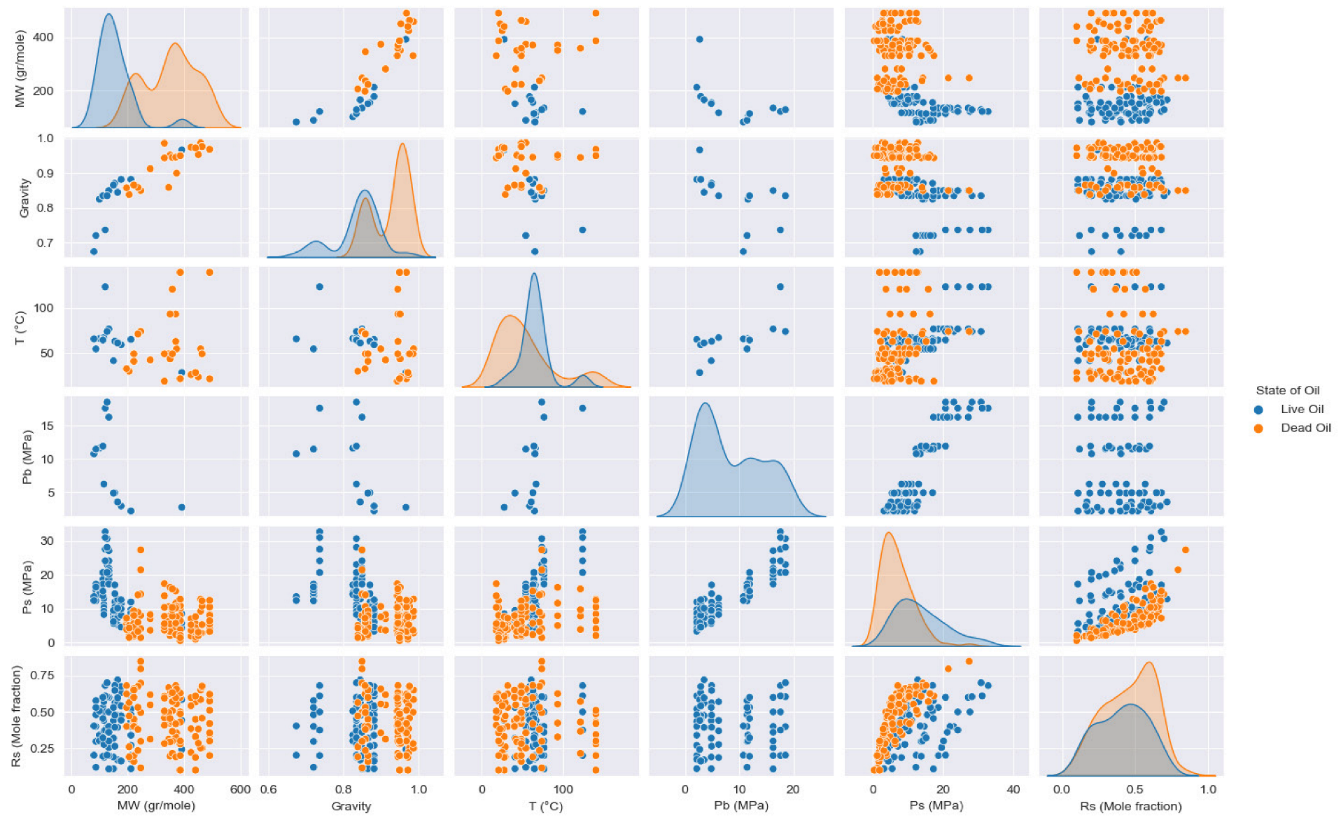
Figure 1. Pair plot of CO2 solubility data for dead oil and live oil.
Eng 04 00108 g001
Figure 2. Rs versus Ps for both models with their linear curves.
Eng 04 00108 g002
Figure 3. Heatmaps of correlation coefficients. (a) dead oil; (b) live oil.
Eng 04 00108 g003
Figure 4. Data distribution for each component.
Eng 04 00108 g004
Figure 5. Data distribution for each parameter.
Eng 04 00108 g005
Figure 6. Pressure–interfacial tension relationship.
Eng 04 00108 g006
Figure 7. The heatmap of correlation coefficients between interfacial tension and the other parameters.
Eng 04 00108 g007
Figure 8. The distribution of data for each parameter.
Eng 04 00108 g008
Figure 9. Boxplot of MMP data. The presence of six outliers (indicated by the six black diamonds) exceeds the right threshold (30 MPa).
Eng 04 00108 g009
Figure 10. Boxplot and histogram of MMP after outliers’ removal.
Eng 04 00108 g010
Figure 11. Heatmap of correlation coefficients between MMP and the other parameters.
Eng 04 00108 g011
Figure 12. Architecture of the MLP-Adam solubility model for dead oil.
Eng 04 00108 g012
Figure 13. Flowchart of the multilayer perceptron using the Adam optimization algorithm for the proposed model.
Eng 04 00108 g013
Figure 14. Comparative plot of predicted and experimental dead solubility values: an analysis of training data, test data, and the complete dataset.
Eng 04 00108 g014
Figure 15. The error histogram of the different correlations [51,52,53].
Eng 04 00108 g015
Figure 16. Plot of predicted versus experimental values of solubility in live oil.
Eng 04 00108 g016
Figure 17. Error histogram of the different correlations [51,52,53].
Eng 04 00108 g017
Figure 18. Flowchart of the proposed XGBoost model.
Eng 04 00108 g018
Figure 19. Importance of inputs in the prediction of IFT.
Eng 04 00108 g019
Figure 20. Plot of predicted versus experimental values of interfacial tension.
Eng 04 00108 g020
Figure 21. Scatter plots of the experimental IFT versus the values predicted by each model.
Eng 04 00108 g021
Figure 22. Scatter plot of the absolute error between predicted and experimental values.
Eng 04 00108 g022
Figure 23. Importance of inputs in MMP prediction.
Eng 04 00108 g023
Figure 24. Plot of predicted versus experimental values of minimum miscibility pressure.
Eng 04 00108 g024
Figure 25. Error histogram of pure XGBoost and the different correlations [48,56,57].
Eng 04 00108 g025
Figure 26. Error histogram of impure XGBoost and the different correlations [38,58].
Eng 04 00108 g026
Table 1. A brief description of the experimental data used for the two solubility models (dead oil and live oil).
Oil StateExperimental DataNo. of SamplesMeanStdMin25%50%75%Max
Dead OilMW (gr/mole)105350.641592.0752196246358424490
γ1050.92570.04810.83820.86540.94520.96770.9867
T (°C)10553.845035.7518.3326.1748.8969.0275140
Ps (MPa)1056.97164.59630.53.54756.029.572527.38
Rs (Mole fraction)1050.45750.17250.10.3130.47890.60480.847
Live OilMW (gr/mole)74152.836461.959880.7115.7133.2173.575391.6
γ740.83710.06170.67480.83480.84980.87890.9663
T (°C)7465.929719.122285964.767123.9
Pb (MPa)748.50525.80592.153.056.211.9118.52
Ps (MPa)7413.62417.16753.238.307512.3317.2432.76
Rs (Mole fraction)740.41030.16770.10830.27160.41820.53810.7201
Table 2. Correlation coefficients between solubility and other parameters.
Oil StateExperimental DataMW (gr/mole)γT (°C)Pb (MPa)Ps (MPa)
Dead OilRs (Mole fraction)−0.0713−0.0934−0.1696-0.7813
Live OilRs (Mole fraction)0.02310.01810.0774−0.01320.3844
Table 3. A brief description of the data used for the interfacial tension model.
Experimental DataNo. Of SamplesMeanStdMin25%50%75%Max
MW (g/mol)1071175.606964.652096134175222275
P (MPa)10716.38484.10640.0973.02569.08517.1
T (K)1071350.699931.6949297.85323.175344.3373.1443.05
IFT (mN/m)10719.83665.85560.0015.2259.3714.1527.05
Table 4. Correlation coefficients between interfacial tension and the other parameters.
Experimental DataMW (gr/mole)P (MPa)T (K)
IFT (mN/m)0.2918−0.8577−0.2042
Table 5. A brief description of the data used for the minimum miscibility pressure model.
Experimental DataNo. of SamplesMeanStdMin25%50%75%Max
TR (K)201345.439524.3101307.55327.59338.71362.040410.37
Tc (K)201302.71788.3058281.45295.29304.19304.190338.77
MWC5+ (g/mol)201194.634840.1033136.26171.1187.80211.213391
xvol/xint2011.59552.092800.510.741.513.6067
MMP (MPa)20116.02356.11846.5011.13814.8019.1238.52
Table 6. Correlation coefficients between MMP and the other parameters.
Experimental DataTR (K)Tc (K)MWC5+ (g/mol)xvol/xint
MMP (MPa)0.6845−0.18290.46570.3133
Table 7. Structure of the proposed MLP-Adam model.
Number of hidden layers2
Number of neurons in the hidden layers12
Number of epochs1000
Optimization algorithmAdam
Activation functionRelu
Performance IndicatorMSE, MAE
Validation dataset16 Samples
Table 8. Statistical analysis of MLP-Adam performance.
ModelTraining DataTest DataAll Data
AARD (%)RMSER2AARD (%)RMSER2AARD (%)RMSER2
MLP-Adam2.01610.01230.99483.96290.02340.98072.30990.01450.9928
Table 9. The comparison between the statistical parameters of MLP-Adam and the different correlations found in the literature.
ModelAARD (%)RMSER2
MLP-Adam2.30990.01450.9928
Chung et al., 1988 [51]99.42130.51380.0083
GA—Emera and Sarma, 2011 [53]6.15210.05460.8987
Rostami et al., 2017 [52]3.87090.020450.9858
Table 10. Search interval and optimal values of the SVR-RBF parameters.
HyperparameterCEpsilonGamma
Range0.1–50,0000.0001–0.10.001–10
Optimal value9500.0390.01035
Table 11. Statistical analysis of SVR-RBF performance.
ModelTraining DataTest DataAll Data
AARD (%)RMSER2AARD (%)RMSER2AARD (%)RMSER2
SVR-RBF2.46180.00880.99724.27420.02090.98352.80470.01200.9948
Table 12. The comparison between the statistical parameters of SVR-RBF and the different correlations found in the literature.
ModelAARD (%)RMSER2
SVR-RBF2.80470.01200.9948
Chung et al. [51]99.92500.44250.0097
GA—Emera and Sarma [53]4.97340.02950.9686
Rostami et al. [52]3.76420.02030.9851
Table 13. Selection of hyperparameters for the proposed XGBoost model of IFT.
ModelHyperparameterRangeOptimal Value
XGBoostNumber of trees100, 200, 400, 800, 1000, 20001000
Regularization parameter λ0.0001, 0.001, 0.1, 0.3, 10, 1000.001
Regularization parameter α0.01, 0.04, 0.09, 0.10.09
Gamma γ0, 0,1, 1, 100
Max. depth2, 4, 6, 84
Learning rate0.001, 0.01, 0.10.1
Table 14. Statistical analysis of XGBoost performance on IFT data.
ModelTraining DataTest DataAll Data
AARD (%)RMSER2AARD (%)RMSER2AARD (%)RMSER2
XGBoost1.93860.09520.99978.64220.46980.99313.28440.22710.9985
Table 15. Statistical comparison of XGBoost and literature-based correlations for the IFT dataset.
ModelAARD (%)RMSER2
XGBoost3.28440.22710.9984
PR EOS60.54712.62610.7949
GEP219.10531.44370.9391
Table 16. Selection of hyperparameters for our XGBoost model of MMP.
ModelHyperparametersRangeOptimal Value
XGBoostNumber of trees100, 1000, 4000, 5000, 80008000
Regularization parameter λ0.0001, 0.001, 0.1, 0.3, 15, 10015
Regularization parameter α0.01, 0.02, 0.09, 0.10.02
Gamma γ0, 0,1, 01, 100
Maximum depth2, 4, 6, 82
Learning rate0.001, 0.01, 0.10.1
Table 17. Statistical analysis of XGBoost performance on MMP data.
ModelTraining DataTest DataAll Data
AARD (%)RMSER2AARD (%)RMSER2AARD (%)RMSER2
XGBoost0.93260.18930.99864.00430.9410.96481.42620.41510.9934
Table 18. Statistical comparison of XGBoost and literature-based correlations for the MMP dataset.
ModelAARD (%)RMSER2
Pure CO2XGBoost (Pure)0.91610.19360.9988
Lee [56]18.7815.15380.5146
Alston et al. (Pure) [48]18.1775.54720.7063
Emera-Sarma [57]13.22033.73850.6161
Impure CO2XGBoost (Impure)1.95250.5580.9856
Alston et al. (Impure) [48]34.53246.46680.5967
Fathinasab-Ayatollahi [58]15.01342.7020.7019
Disclaimer/Publisher’s Note: The statements, opinions and data contained in all publications are solely those of the individual author(s) and contributor(s) and not of MDPI and/or the editor(s). MDPI and/or the editor(s) disclaim responsibility for any injury to people or property resulting from any ideas, methods, instructions or products referred to in the content.