Abstract
Using surrogate safety measures is a common method to assess safety on roadways. Surrogate safety measures allow for proactive safety analysis; the analysis is performed prior to crashes occurring. This allows for safety improvements to be implemented proactively to prevent crashes and the associated injuries and property damage. Existing surrogate safety measures primarily rely on data generated by microsimulations, but the advent of connected vehicles has allowed for the incorporation of data from actual cars into safety analysis with surrogate safety measures. In this study, commercially available connected vehicle data are used to develop crash prediction models for crashes at intersections and segments in Salt Lake City, Utah. Harsh braking events are identified and counted within the influence areas of sixty study intersections and thirty segments and then used to develop crash prediction models. Other intersection characteristics are considered as regressor variables in the models, such as intersection geometric characteristics, connected vehicle volumes, and the presence of schools and bus stops in the vicinity. Statistically significant models are developed, and these models may be used as a surrogate safety measure to analyze intersection safety proactively. The findings are applicable to Salt Lake City, but similar research methods may be employed by researchers to determine whether these models are applicable in other cities and to determine how the effectiveness of this method endures through time.
1. Introduction
Surrogate safety measures (SSMs) offer benefits over traditional safety analysis methods that use historical crash data. SSMs are a type of safety analysis that make use of data other than crash data, typically vehicle kinematic data. The first benefit of SSMs is that they use data which may be collected more rapidly than historical crash data. Crashes are rare events, and historical data may require years of accumulation to conduct a safety analysis. The second benefit is that SSM analysis is proactive, allowing for safety analysis prior to crashes occurring. An unsafe location may therefore be identified and improved before crashes occur, preventing injuries and property damage and possibly saving lives. The third benefit of SSMs is that the kinematic data used in a safety analysis with SSMs are much more voluminous, allowing for statistical methods to be more effective.
The kinematic data employed by SSMs may come from several sources. In the past, manual measurement at the study site was used. This method of data collection was problematic because it allowed for subjectivity and was difficult to perform accurately due to the fleeting nature of traffic interactions. Manual observation was replaced with video recordings which made it possible for traffic interactions to be replayed and offered the chance for multiple observers to analyze interactions, thus improving the problem of subjectivity. This problem has been further ameliorated with automated video data reduction with technology such as that offered by Transoft, Iteris, and similar companies. Additionally, microsimulation technology has allowed for simulation to be used as a source of kinematic data. This method eliminates subjectivity, as the computer running the simulation provides the data rather than human observers [1]. Microsimulation produces highly detailed and precise data and can produce large volumes of data with relatively little effort in comparison with manual collection. The fault of microsimulation lies in it being an abstraction rather than reality. While microsimulations are still highly useful, there has been research into the use of connected vehicle (CV) data with SSMs, meaning the use of data from the physical world rather than simulation.
CVs are a source of traffic data that allows for the high level of precision offered by microsimulation along with the realism of being generated by human drivers. CVs are automobiles sold to the public that include a transceiver which allows data to be collected regarding the vehicle’s motion. For the sake of privacy, no individually identifiable information about the vehicle is visible. Vendors offer CV data to clients who wish to use the data for research and engineering projects. The main drawback of using data from CVs is that they currently comprise a small percentage of the total number of vehicles in the United States. A study from October 2021 found the median CV penetration rate to be approximately 4.5% [2]. Therefore, CVs do not offer a full picture of traffic. They are gradually becoming more common, though, as older vehicles are retired and replaced with new vehicles that are connected. Research into effective analysis methods with CV data will become more valuable as time goes on, speaking to the need for this research to take place now for a future increase in CVs.
One metric that is available from CVs is harsh braking event counts, which form the basis for the models developed in this study. Data points from CVs include information about braking and acceleration. The braking data may be filtered so that harsh braking events are identified and counted and then used as a regressor variable in a crash prediction model. This method is investigated in this paper. The significance of other regressor variables, such as CV volume and intersection geometric characteristics, was also investigated. The proposed crash prediction models may be used to estimate monthly counts of intersection-related crashes and offer all of the benefits of SSMs mentioned above.
The statistical models developed in this study show promise for use as a surrogate safety measure. Of the twelve statistical models developed in this study, ten possess a high level of statistical significance. Although connected vehicle penetration rates are too low at this time to depend upon models such as these, once these penetration rates increase, these models will offer an additional method of analysis.
1.1. Literature Review
Researchers have developed many SSMs which tend to fall into three categories. SSMs can be a time-based measure, a deceleration-based measure, or a safety index. Although most SSMs consider collisions involving two vehicles, it is possible to model single-vehicle crashes due to distraction or error [3]. SSMs operate upon the concept that events with greater risk tend to happen less frequently, with the riskiest and rarest events being the events that result in collision [4]. By analyzing less risky events that occur significantly more frequently, a safety analysis with SSMs can offer more insight into safety than an analysis with crash data alone.
1.1.1. Time-Based Measures
Time-based measures consider the kinematics of vehicles and how much of a time gap exists between vehicles. Time-to-collision (TTC), post-encroachment time (PET), and proportion of stopping distance (PSD) are time-based SSMs. TTC is a measure of the amount of time required for the space between two vehicles to close. TTC on its own is transient, but Minderhoud and Bovy developed aggregation methods in the form of their extended TTC measures, namely time-integrated TTC and time-exposed TTC [5]. Post-encroachment time is the difference in time between when an encroaching vehicle exits the path of travel and when a following vehicle first occupies the location where a collision would have occurred. A modified form of PET exists as initially attempted PET (IAPE). IAPE corrects the measure to account for the acceleration that commonly occurs when a driver determines that a conflict has ended [6]. PSD is a ratio between the distance a vehicle is from a potential collision location and the minimum stopping distance. These distances depend upon the velocity of the vehicles involved, making PSD a time-based measure.
There are both strengths and weaknesses associated with time-based SSMs. The strength of time-based SSMs lies in their simplicity and intuitiveness. TTC and PET may be implemented with kinematic data supplied by either on-site measurements or microsimulation. PSD also requires such kinematic data, but it also requires information on the vehicles’ possible deceleration rates. This deceleration rate can be an established value or distribution of values or may be derived from environmental conditions. Drivers are aware of the importance of following distance and time headway, making these measures intuitive for researchers and practitioners alike. A weakness of time-based SSMs is the possibility of multiple encounters producing identical measures [7]. TTC may evaluate the same solution for both an encounter with a large speed differential between vehicles and a long following distance and another encounter with a small speed differential but a short following distance. This has made it difficult to establish particularly meaningful safety thresholds for these measures. Another weakness is the inability of time-based SSMs to evaluate the severity of a potential collision. In the encounters just described, which both result in an identical TTC, the severity of a resulting collision will be very different due to the differing speed differentials.
1.1.2. Deceleration-Based Measures
Deceleration-based measures consider braking action and the braking capacity of vehicles and are better equipped than time-based measures to evaluate potential crash severity. Additionally, this type of measure considers a driver’s evasive action, an important component of traffic conflicts. Deceleration-based measures include braking applications and deceleration rate to avoid collision (DRAC). Brake applications have been found to be a poor SSM due to the variability in braking habits among drivers. Brake applications are such a common act, even in benign situations, that they are not highly indicative of a conflict [6]. Brake applications as an SSM fail to consider the severity of each particular braking action, something that DRAC and harsh braking are able to capture to their benefit. DRAC is a measure of the deceleration rate that a following vehicle would need to apply to avoid colliding with a leading vehicle. This measurement is compared to a safety threshold, commonly given as 3.35 m/s2, to determine whether a conflict occurred [8].
Harsh braking events have also been suggested as an indicator of a conflict, which would also fall under the category of deceleration-based measures. A 2015 study found a high level of correlation between crash counts and harsh braking events, defined as events with a large absolute value of the first derivative of acceleration, known as jerk. These events were collected by vehicles with GPS units which collected data on the vehicles’ location over time, allowing the jerk value to be computed. Mousavi found a threshold of −0.762 m/s3 to be the most effective to define harsh braking but also noted that this threshold is lower than expected. Further investigation of a proper jerk threshold was recommended [9].
1.1.3. Safety Indices
Safety indices are the third category of SSM. These indices consider various factors and produce an indirect safety metric. Two examples are crash potential index (CPI) and the aggregated crash propensity metric (ACPM). CPI was developed to improve upon the drawbacks of the DRAC measure. While a constant safety threshold value is typically used with DRAC, the braking capacity of vehicles is variable for mechanical and environmental reasons. CPI considers this variability through the use of a maximum available deceleration rate (MADR) distribution. The probability that DRAC is greater than MADR is a term in the computation of CPI. ACPM also considers the MADR distribution in conjunction with a distribution of driver reaction times to compute the probability that each vehicle interaction will result in collision. These probabilities are aggregated to produce the ACPM [10]. CPI and ACPM indicate the safety level of a study location and time period without being a single measure of some observable quality.
Of the SSMs discussed, the analysis of harsh braking events holds potential due to its compatibility with CV data. Previous studies, such as Mousavi’s thesis [9] and the work of Bagdadi and Varhelyi [11], have analyzed harsh braking data from GPS units due to the lack of availability of large-scale CV data when these studies were conducted. He et al. investigated the use of CV data for SSMs, using a safety pilot model dataset to compute TTC, DRAC, and a modified form of TTC [12]. Their study demonstrated the effectiveness of computing these measures with kinematic data from CVs. The development of a crash prediction model that uses harsh braking data from CVs would bridge the gap between these two studies and provide another tool for safety analysis.
2. Materials and Methods
The methods undertaken in this study include the three following phases: selection of study intersections, data collection, and statistical modeling. CV data collection was enabled by the automobile companies that manufactured the CVs. This study uses data within Salt Lake City, Utah for the months of March 2019, January 2021, and August 2021. These months were selected due to the availability of CV data for these particular months. A larger sample size in future studies would be preferable, but there were only three months of CV data due to budgetary restrictions.
2.1. Intersection Selection
The intersection selection process involved the collection of crash counts for all major intersections in Salt Lake City, amounting to 370 intersections. Crash counts for the three study months were obtained from the UDOT database and summed to find the total number of crashes for the intersections. The crashes within the UDOT system were filtered to include only those deemed to be intersection related by law enforcement. The sixty intersections with the most crashes were selected. The total monthly crashes ranged from zero to six. The sixty chosen study intersections included both signalized and unsignalized intersections.
2.1.1. Data Collection
The CV data interface comprises an interactive map and a control pane. The map displays waypoints that are produced by the CVs. When a CV is in motion, waypoints are produced once every three seconds. The waypoints are grouped by the overall trip of which it is a part by a journey ID number, making it possible to collect CV volumes. The waypoints also include data such as geographical location, a timestamp, speed, acceleration, jerk, heading, and information about the origin and destination of the trip that includes the particular waypoint. Harsh braking events were identified using the jerk values of these waypoints. Jerk is the first derivative of acceleration and is recorded for each of the waypoints. Jerk is a continuous measure for a vehicle, similar to speed or location. Each waypoint contains a value for jerk at the particular moment corresponding to the waypoint. This value is derived from the speed data. A geospatial filter was applied to limit the waypoints to those within the influence area of the study intersections, the main intersection square, and the legs of the intersection 250 ft behind the stop bar as displayed in Figure 1 [13]. Another filter was applied to limit waypoints to only those that possess a jerk value that is above the threshold that differentiates a regular braking event from a harsh braking event. This jerk threshold varied in this study to test the effectiveness of several harsh braking definitions. Thresholds tested varied between −0.15 m/s3 and −3.2 m/s3 in increments of 0.15 m/s3. The query tool was used to obtain counts of harsh braking events for each of the jerk thresholds.
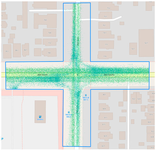
Figure 1.
Intersection influence area with waypoints displayed.
Other metrics collected from the CV data included the CV volumes and the average jerk value for each of the intersections. The CV volumes were obtained by querying the unique count of the journey ID numbers. This counts the number of groups of waypoints that belong to trips that pass through the intersection. Thus, the volume of vehicles passing through the intersection is obtained. The total monthly CV volume was collected as was the total monthly volume that used the intersection between the hours of 7 AM and 9 AM and between the hours of 4 PM and 6 PM. The average jerk value among all waypoints within the intersection influence area was obtained on a monthly basis for each of the three study months for each of the intersections.
In addition to the crash data and CV data, information regarding the geometry and geography of each of the intersections was collected. The number of approaches with left turn lanes, the number of approaches with right turn lanes, and the maximum number of lanes that a pedestrian would have to cross were collected using Google Earth. Historical imagery was employed to ensure that these values were correct for the study months in question. ArcGIS Pro was used to determine the number of bus stops and the number of schools within a 305 m radius of the center point of each of the intersections. These metrics were included in this study because they are used in the safety performance functions within the Highway Safety Manual [14]. Table 1 is a summary of the dependent, exposure, and regressor variables collected for analysis in this study as organized per intersection or segment per month.

Table 1.
Summary of variables.
2.1.2. Statistical Analysis
Once these data points were collected for each of the study intersections during each of the study months, a statistical regression analysis was performed to produce crash prediction models for Salt Lake City. Poisson regression, negative binomial regression, and generalized Poisson regression were considered in the analysis. Three statistical methods were used for the sake of producing a larger number of total models and investigating which of the regression methods performed best. Poisson regression requires that the mean and variance are equal for the dependent variable in the regression. The mean and variance of the monthly crashes at the intersections were approximately equal, making Poisson regression a viable option.
Poisson Regression
Poisson regression is applicable when the variable of interest is assumed to follow the Poisson distribution, which is a model of the probability that a particular number of events will occur. The dependent variable is the event count, which can be any of the nonnegative integers. Large counts are assumed to be uncommon, making Poisson regression similar to logistic regression, with a discrete response variable. Poisson regression, unlike logistic regression, does not limit the response variable to specific values. The Poisson distribution model takes the form given in Equation (1), in which Y is the dependent variable, y is a count from among the nonnegative integers, and μ is the mean incidence rate for an event per unit of exposure.
If the Poisson incidence rate, μ, is assumed to be determined by a set of regressor variables, then Poisson regression is possible through the expression displayed in Equation (2) and the regression model displayed in Equation (3). In these equations, X is a regressor variable, β is a regression coefficient, and t is the exposure variable.
The regression coefficients in Equation (2) may be estimated by maximizing the log-likelihood for the regression model. This is achieved by setting the derivative of the log-likelihood equal to zero to generate a system of nonlinear equations which may be solved with an iterative algorithm. The reweighted least squares iterative method is typically able to converge to a solution within six iterations [15].
Negative Binomial Regression
The negative binomial distribution is a generalization of the Poisson distribution that includes a gamma noise variable. This allows for negative binomial regression to be performed even if the dependent variable’s mean and variance are not equal [16]. Negative binomial regression is commonly used for traffic safety applications because it has loosened restrictions in comparison to Poisson regression but is still capable of estimating an observed count, such as crash counts [17]. The negative binomial distribution takes the form presented in Equation (4), in which α is the reciprocal of the scale parameter of the gamma noise variable and other variables are as defined previously.
The mean of y in negative binomial regression depends upon the exposure variable and the regressor variables which are related by the expression displayed in Equation (5). Negative binomial regression is possible with the regression model displayed in Equation (6). In these equations, x is a regressor variable, and the other variables are as defined previously. As with Poisson regression, maximizing the log-likelihood may be used to estimate the regressor coefficients through an iterative algorithm [16].
Generalized Poisson Regression
Generalized Poisson regression, like negative binomial regression, is applicable in a broader set of circumstances than Poisson regression. This is because it does not have the requirement that the mean and variance of the dependent variable in the regression be equal. There are two types of generalized Poisson regression models: Consul’s generalized Poisson model and Famoye’s restricted generalized Poisson regression model. Consul’s model, also known as the Generalized Poisson-1 (GP-1) model, is the regression model that was employed in this study. The GP-1 model operates on the assumption that the dependent variable, y, is a random variable following the probability distribution presented in Equation (7), in which λ is the number of events per unit of time and α is the dispersion parameter which can be estimated using Equation (8) [18]. In Equation (8), N is the number of samples, k is the number of regression variables, yi is the ith observed value, and ŷi is the Poisson rate λi predicted for the ith sample [19].
Poisson, negative binomial, and GP-1 regression techniques were explored by model generation in R. Models with many different combinations of regressor variables were created to find the model that performed best. In all models, the number of monthly crashes was used as the dependent variable, and the monthly CV volume was used as the exposure variable. The statistical models were evaluated based on the significance of the regressor variables used in the models, on the basis of the Akaike Information Criterion, and based on the residuals generated by the models. The best-performing models were selected and are summarized and discussed in the Results and Discussion Sections.
2.2. Segment Analysis
The preliminary results from the intersection study prompted interest in how the results of an intersection-based study would compare to the results of a segment-based study. To address this, a segment analysis was conducted. CV data were collected for thirty road segments in the Salt Lake City area. These segments include sections of interstate highway within the Salt Lake City limits and sections of interrupted state highway outside of the influence area of any intersections. The segments were all made to be approximately one-quarter mile in length to ensure that the segments had roughly equal exposure to crashes occurring. This prevented the need to determine a crash rate per unit length.
The segment CV data were collected in the same manner as the intersection CV data with a couple of key differences. First, the intersection CV data were all collected from within intersection influence areas. The segment CV data were all collected from areas entirely outside of intersection influence areas. Second, the geometric information and information related to schools and bus stops were not collected for the segments. Rather, the segment data included only harsh braking events for jerk thresholds ranging between −0.3 m/s3 and −3.0 m/s3 in increments of 0.3 m/s3, as well as monthly CV counts, monthly CV counts between the hours of 7 AM and 9 AM, and monthly CV counts between the hours of 4 PM and 6 PM. As with the intersection analysis, crash data were collected for the segments from the UDOT database. The increment between successive jerk thresholds for segments differs from that which was used for intersections. This was done simply for the purpose of decreasing the amount of work needed for the analysis. More thresholds could have been tested, but the preliminary results from the intersection study indicated that the increment did not need to be as fine as 0.15 m/s3. Table 2 is a summary of the variables collected for segments in this study.
Table 2.
Summary of segment variables.
Statistical analysis was conducted in the same manner as the intersection analysis, with Poisson, negative binomial, and generalized Poisson models generated and evaluated for the segment dataset. The best-performing models were selected and are summarized and discussed in the following sections.
3. Results
The collected intersection data were used for a statistical regression analysis, and the best regression model for each of the model families was found that had a high level of significance among the regressor variables and the intercept. The best Poisson model uses Jerk18 and Schools from Table 1 as regressor variables. The best negative binomial model also uses Jerk18 and Schools as regressor variables. The best generalized Poisson model uses Jerk18 as a regressor variable. All of these models have a better than 0.1% significance level for their regressor variables and the intercept. In the case of the generalized Poisson model, both intercepts are significant at a better than 0.1% level. These models are summarized in Table 3.
Table 3.
Summary of regression models for intersection analysis.
The segment analysis also yielded three statistical models: a Poisson regression model, a negative binomial regression model, and a generalized Poisson regression model. The best Poisson, negative binomial, and generalized Poisson models identified use Jerk2 as a regressor variable. All models have a better than 0.1% significance level for their regressor variable and intercept(s). These models are summarized in Table 4.
Table 4.
Summary of regression models for segment analysis.
The estimates for the coefficients of the harsh braking variable in each of these regression models (Jerk18 and Jerk2) are all negative, indicating that an increase in hard braking events decreases the estimate for the number of crashes that will occur within the intersection area or along the segment in question. This suggests that hard braking events are an indication of safety. This is true at intersections as well as on segments away from the influence of intersections.
Table 3 and Table 4 include the models with the best level of statistical significance, but there were numerous other models identified which also were statistically significant. A number of potential models could theoretically be used with similar results. The models display a gradual degradation in significance as the jerk variable used gets further away from the Jerk18 variable for intersections and the Jerk2 variable for segments.
Validation efforts conducted with the models produced the following graphs, displayed in Figure 2 and Figure 3. These graphs display the expected monthly crash counts for each of the three models on the vertical axis. The horizontal axis represents the observed monthly crash counts that correspond to each of the expected crash counts. The “jitter” function in R has been used to generate these plots; hence, there is scatter around the integer counts of observed crashes.

Figure 2.
Intersection fitted crash counts versus observed crash counts.

Figure 3.
Segment fitted crash counts versus observed crash counts.
An additional analysis was conducted in the same manner as that which yielded the results presented up to this point, except with outlier crash counts removed from the intersection and segment datasets. The outliers were identified using boxplots generated for the observed crash counts. These boxplots are presented in Figure 4. The outliers are denoted as black points in Figure 4. The best identified Poisson, negative binomial, and generalized Poisson models are summarized in Table 5 and Table 6.
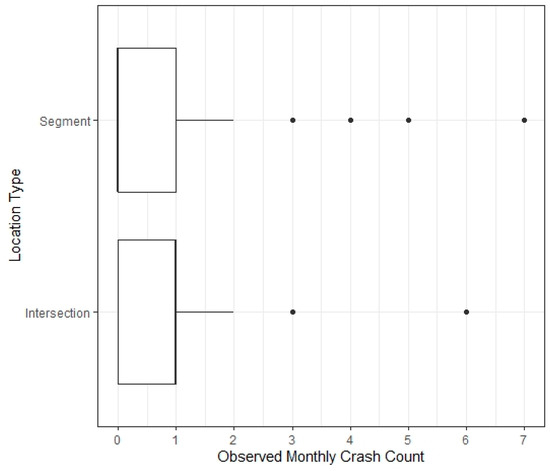
Figure 4.
Boxplots of the observed monthly crash counts at intersections and segments.
Table 5.
Summary of regression models for intersection analysis with outliers removed.
Table 6.
Summary of regression models for segment analysis with outliers removed.
Validation efforts were conducted for the models generated with outlier crash counts removed from the datasets. These validation efforts produced the graphs displayed in Figure 5 and Figure 6. These graphs display the expected monthly crash counts for each of the three models on the vertical axis. The horizontal axis represents the observed monthly crash counts that correspond to each of the expected crash counts.

Figure 5.
Intersection fitted crash counts versus observed crash counts with outliers removed.

Figure 6.
Segment fitted crash counts versus observed crash counts with outliers removed.
4. Discussion
This study demonstrates the effectiveness of using harsh braking data from CVs as a surrogate safety measure. For both intersections and segments, statistically significant models may be developed from multiple model families. Models such as these may be used to predict future crash rates for the purposes of prioritizing improvements and identifying risks to the public.
The results of this study reveal the jerk threshold for intersections and segments. For intersections, the jerk threshold is −2.7 m/s3, corresponding to the regressor variable Jerk18. This threshold was identified to be the most effective for all three statistical model families. The jerk threshold for segments was found to be −0.3 m/s3, corresponding to the variable Jerk2. A jerk threshold of −2.7 m/s3 for intersections and −0.3 m/s3 for segments indicates that intersections and segments operate differently in terms of safety. The jerk threshold is the value of jerk that differentiates ordinary events from harsh braking events. Events that do not meet the jerk threshold have little or no bearing on crash prediction. A larger absolute value of jerk threshold for intersections over segments indicates that braking must be more severe at an intersection to qualify a braking event as harsh. This could be due to different expectations of drivers in these differing contexts. At intersections, drivers expect to brake and are typically able to see the status of the traffic signal well in advance. Moderately hard braking, such as an event that generates a jerk value of −1.5 m/s3, is expected and therefore ordinary. Such an event in a segment context, however, would be relatively unexpected and therefore extraordinary because segments are expected to have more uniform and smooth flow. This event would therefore qualify as a harsh braking event in a segment context but not in an intersection context.
The coefficient estimates for the harsh braking event count variables were found to be negative for all statistical models generated, indicating that an increase in harsh braking events is correlated with an increase in the frequency of zero crashes and a decrease in the frequency of one or more crashes. This means that harsh braking is correlated with increased safety on roads. The coefficient estimates for the jerk variable are small relative to other covariates, when the covariates are statistically significant. The small value for these coefficient estimates is due to the number of crashes being a small number relative to the high jerk event counts, as can be seen in Table 1 and Table 2. To obtain a crash count estimate from a high jerk event count requires that the coefficient estimate be quite small. This study was predicated upon the notion that a harsh braking event corresponds to a traffic conflict and that traffic conflicts and collisions are related. That these models have negative estimates for the coefficients of the harsh braking event counts suggests that harsh braking events are indicative of the prevention of a traffic conflict which leads to the increase in the probability of zero crashes and to the increase in the probability of one or more crashes. Harsh braking events are events which might have been collisions but never were as a result of the evasive action of the drivers involved.
The statistical models presented in Table 3 and Table 4 possess an excellent level of statistical significance at a level better than 0.1%. Poisson models are simpler than negative binomial models and generalized Poisson models, making them preferable if applicable. While the requirement that the mean and variance of the dependent variable be equal was approximately satisfied for the dataset used in this study, that may not be the case for other datasets. Therefore, negative binomial and generalized Poisson regression are recommended for crash prediction models based on harsh braking data.
As mentioned above, the presence of schools was found to increase crash frequency within intersection influence areas. This confirms the efficacy of the use of school presence in HSM safety analysis methodology. The estimated coefficients for the Schools variable are positive, indicating that the presence of a school or multiple schools nearby decreases the frequency of zero crashes and increases the frequency of one or more crashes. The presence of schools increases pedestrian activity and the presence of young drivers, which may help explain this increase.
The graphs presented in Figure 2 and Figure 3 illustrate that these models fail to predict high crash counts while performing better at locations with lower numbers of observed crashes. This was not unexpected because the count models used in this study predict low probabilities for higher counts. The statistical significance of the regressor variables in the models, on the other hand, speaks to their overall strength. As CV penetration rates increase, allowing models based on CV data to be trained by a fuller picture of the activity on roads, models of this form will likely become more effective. Preliminary studies such as this, using CV data information in its technological infancy, set the stage for a future in which CVs become significantly more widespread and CV data capture a large portion if not a majority of roadway traffic. Figure 5 and Figure 6, as well as the RMSE values presented in Table 5 and Table 6 demonstrate that the models’ predictive ability improves when outliers are removed. The RMSE values for intersections decreased from approximately 0.95 to 0.63 for intersections and from approximately 1.55 to 0.76 for segments. The decrease in RMSE indicates that the models produce more accurate crash count estimates when outliers are removed.
5. Conclusions
This study developed several statistical models which use harsh braking event counts from CV data in Salt Lake City as regressor variables and crash counts as the dependent variables. Both intersections and segments were considered separately in this study with models derived for each. Poisson, Negative Binomial, and Generalized Poisson models were developed and they revealed the jerk threshold for intersection influence areas to be −2.7 m/s3 and the jerk threshold for segments to be −0.3 m/s3. Additionally, the presence of schools within 305 m was found to be a statistically significant variable for intersection influence areas.
Crash prediction models such as these, based on harsh braking event counts, hold promise for agencies and industry as another tool for safety analysis. Agencies may investigate these models and tailor them to their jurisdictions for the purpose of adding such models to their established methodologies. Such tailored models may then be employed as a means of conducting comparative safety analysis for the purpose of identifying crash-prone locations and prioritizing improvements. Once a particular area is identified as being crash prone, further investigation into the cause of the safety hazard may commence. Employing harsh braking models such as those developed in this study requires less labor investment than existing methods, allowing for more frequent and widespread analyses to identify and characterize road hazards. It should be noted that the intersection models developed in this research are likely not applicable to sites with low crash activity, as intersections were selected to maximize the amount of historical crash activity.
Future research into SSMs that are based on harsh braking events could include the investigation of regional differences in models, the use of additional regressor variables in segment-based models, and harsh positive acceleration data from CVs. Regional differences may exist pertaining to the relationship between harsh braking and collisions. Harsh braking events were found to be positively correlated to crashes in a previous study in Louisiana which is contrary to the findings of this study [9]. While this may be due to the significant differences in the methods of data collection between these two studies, regional variations may also be a factor and ought to be investigated further. Additional regressor variables were not investigated in the segment-based models developed in this study to the degree to which they were investigated in the intersection-based models. The inclusion of such additional regressor variables for segments ought to be investigated more fully in a future study. These variables may include speed limits, curvature parameters, lane widths, or total number of lanes, among others. Finally, harsh positive acceleration data may be obtained in the same manner in which harsh braking data were collected in this study. Harsh acceleration may be an indicator of safety or the lack thereof because it can represent erratic driving behavior or situations in which a driver is attempting to clear a potential crash location rapidly. The consideration of harsh acceleration data may be performed separately from harsh braking data or in combination with harsh braking data. If attempts are successful, this would yield yet another tool for agencies and industry to employ for surrogate safety analysis.
Author Contributions
The authors confirm contribution to the paper as follows: study conception and design: M.K.; data collection: N.E.; analysis and interpretation of results: M.K. and N.E.; manuscript preparation: N.E. and M.K. All authors have read and agreed to the published version of the manuscript.
Funding
This research was partially funded by Subaward No. UWSC9924 from the University of Washington to Boise State University from the U.S. Department of Transportation award to the University of Washington.
Data Availability Statement
Data used in this research are available by contacting the corresponding author at mkhanal@boisestate.edu.
Acknowledgments
The authors are grateful to the Boise State University Department of Civil Engineering for their support of this research. The authors would also like to express their gratitude to the support received from the PacTrans Region 10 University Transportation Center that made the procurement of the CV data possible.
Conflicts of Interest
The authors declare no conflict of interest.
References
- Gettman, D.; Head, L. Surrogate Safety Measures from Traffic Simulation Models Final Report; U.S. Department of Transportation Federal Highway Administration Office of Research, Development, and Technology: Washington, DC, USA, 2003. [CrossRef]
- Hunter, M.; Mathew, J.K.; Li, H.; Bullock, D.M. Estimation of Connected Vehicle Penetration on US Roads in Indiana, Ohio, and Pennsylvania. J. Transp. Technol. 2021, 11, 597–610. [Google Scholar] [CrossRef]
- Astarita, V.; Caliendo, C.; Giofrè, V.P.; Russo, I. Surrogate Safety Measures from Traffic Simulation: Validation of Safety Indicators with Intersection Traffic Crash Data. Sustainability 2020, 12, 6974. [Google Scholar] [CrossRef]
- Tarko, A.P. Use of Crash Surrogates and Exceedance Statistics to Estimate Road Safety. Accid. Anal. Prev. 2012, 45, 230–240. [Google Scholar] [CrossRef]
- Minderhoud, M.M.; Bovy, P.H. Extended Time-to-Collision Measures for Road Traffic Safety Assessment. Accid. Anal. Prev. 2001, 33, 89–97. [Google Scholar] [CrossRef] [PubMed]
- Allen, B.L.; Shin, B.T.; Cooper, D.J. Analysis of Traffic Conflicts and Collisions. Transp. Res. Rec. 1978, 667, 67–74. [Google Scholar]
- Souza, J.Q.; Sasaki, M.W.; Cunto, F.J.C. Comparing Simulated Road Safety Performance to Observed Crash Frequency at Signalized Intersections. In Proceedings of the International Conference on Road Safety and Simulation, Indianapolis, IN, USA, 14–16 September 2011. [Google Scholar]
- Guido, G.; Saccomanno, F.; Vitale, A.; Astarita, V.; Festa, D. Comparing Safety Performance Measures Obtained from Video Capture Data. J. Transp. Eng. 2010, 137, 481–491. [Google Scholar] [CrossRef]
- Mousavi, S.M. Identifying High Crash Risk Roadways through Jerk-Cluster Analysis. Master’s Thesis, Louisiana State University, Baton Rouge, LA, USA, 2015. Available online: https://digitalcommons.lsu.edu/gradschool_theses/159 (accessed on 15 February 2022).
- Wang, C.; Stamatiadis, N. Surrogate Safety Measure for Simulation-Based Conflict Study. Transp. Res. Rec. 2013, 2386, 72–80. [Google Scholar] [CrossRef]
- Bagdadi, O.; Várhelyi, A. Jerky driving—An indicator of accident proneness? Accid. Anal. Prev. 2011, 43, 1359–1363. [Google Scholar] [CrossRef] [PubMed]
- He, Z.; Qin, X.; Liu, P.; Sayed, M.A. Assessing Surrogate Safety Measures Using a Safety Pilot Model Deplayment Dataset. Transp. Res. Rec. 2018, 2672, 1–11. [Google Scholar] [CrossRef]
- Highway Capacity Manual, Sixth Edition: A Guide for Multimodal Mobility Analysis; Transportation Research Board, National Research Council: Washington, DC, USA, 2016.
- Highway Safety Manual; American Association of State Highway and Transportation Officials: Washington, DC, USA, 2010.
- Poisson Regression. NCSS Statistical Software. Available online: https://ncss-wpengine.netdna-ssl.com/wp-content/themes/ncss/pdf/Procedures/NCSS/Poisson_Regression.pdf (accessed on 5 May 2022).
- Negative Binomial Regression. NCSS Statistical Software. Available online: https://ncss-wpengine.netdna-ssl.com/wp-content/themes/ncss/pdf/Procedures/NCSS/Negative_Binomial_Regression.pdf (accessed on 5 May 2022).
- Wang, J.; Huang, H.; Zeng, Q. The effect of zonal factors in estimating crash risks by transportation modes: Motor vehicle, bicycle and pedestrian. Accid. Anal. Prev. 2017, 98, 223–231. [Google Scholar] [CrossRef] [PubMed]
- Hilbe, J.M. Negative Binomial Regression, 2nd ed.; Cambridge University Press: Cambridge, UK, 2011. [Google Scholar] [CrossRef]
- Date, S. Time Series Analysis, Regression and Forecasting: The Generalized Poisson Regression Model. Available online: https://timeseriesreasoning.com/contents/generalized-poisson-regression-model/ (accessed on 10 July 2022).
Disclaimer/Publisher’s Note: The statements, opinions and data contained in all publications are solely those of the individual author(s) and contributor(s) and not of MDPI and/or the editor(s). MDPI and/or the editor(s) disclaim responsibility for any injury to people or property resulting from any ideas, methods, instructions or products referred to in the content. |
© 2023 by the authors. Licensee MDPI, Basel, Switzerland. This article is an open access article distributed under the terms and conditions of the Creative Commons Attribution (CC BY) license (https://creativecommons.org/licenses/by/4.0/).